Exploring the R CrA environment with SPHERE:

Abstract

Aims. R Coronae Australis (R CrA) is the brightest star of the Coronet nebula of the Corona Australis (CrA) star forming region. It has very red colors, probably due to dust absorption and it is strongly variable. High contrast instruments allow for an unprecedented direct exploration of the immediate circumstellar environment of this star.

Methods. We observed R CrA with the near-IR channels (IFS and IRDIS) of SPHERE at VLT. In this paper, we used four different epochs, three of them from open time observations while one is from the SPHERE guaranteed time. The data were reduced using the DRH pipeline and the SPHERE Data Center. On the reduced data we implemented custom IDL routines with the aim to subtract the speckle halo. We have also obtained pupil-tracking H-band (1.45-1.85 $\mu$m) observations with the VLT/SINFONI near-infrared medium-resolution (R$\sim$3000) spectrograph.

Results. A companion was found at a separation of 0.156^′′ from the star in the first epoch and increasing to 0.184^′′ in the final one. Furthermore, several extended structures were found around the star, the most noteworthy of which is a very bright jet-like structure North-East from the star. The astrometric measurements of the companion in the four epochs confirm that it is gravitationally bound to the star. The SPHERE photometry and the SINFONI spectrum, once corrected for extinction, point toward an early M spectral type object with a mass between 0.3 and 0.55 M_⊙. The astrometric analyis provides constraints on the orbit paramenters: e$\sim$0.4, semi-major axis at 27-28 au, inclination of $\sim 70^{\circ}$ and a period larger than 30 years. We were also able to put constraints of few M_Jup on the mass of possible other companions down to separations of few tens of au.

1 Introduction

Nowadays young stars surrounded by a protoplanetary disk are considered as the primary environment where studying the formation of giant exoplanets (see e.g. Chen et al. 2012; Marshall et al. 2014). In addition, it is clear that giant planets at large separations are more frequently found around intermediate mass stars than around solar-mass stars (see e.g. Johnson et al. 2010; Bowler 2016). Herbig AeBe (HAeBe) stars (Herbig 1960; Hillenbrand et al. 1992) are young ($<$10 Myr), intermediate mass (1.5-8M_⊙) and typically with A, B, F spectral types. They are characterized by a strong infrared excess (The 1994) due to the presence of a circumstellar protoplanetary disk. They are also experiencing accretion processes and their spectral line profiles are very complex. These characteristics make these objects very valuable in the field of extrasolar planets given that they allow to explore the very first stages of the formation of planetary systems.

The HAeBe star R Coronae Australis (R CrA - HIP 93449) is the brighest star in the very young, compact ($\sim$1 pc in diameter) and obscured Coronet protostar cluster (Taylor & Storey 1984). This cluster is characterized by a very high and spatially variable extinction with $A_{V}$ up to 45 mag (Neuhäuser & Forbrich 2008). This nebula is located toward the center of the Corona Australis (CrA) molecular clouds complex (Graham 1992), one of the nearest star forming region with a distance of $\sim$130 pc (Neuhäuser & Forbrich 2008). More recently, Dzib et al. (2018), using the mean trigonometric parallax obtained from Gaia Data Release 2 (Gaia Collaboration 2018), estimated a distance of $154\pm 4$ pc. The presence of emission line objects was also signaled in the vicinity of R CrA(Graham 1993). The CrA region was explored through deep infrared imaging by Wilking et al. (1997) that identified hundreds of point-like sources. Moreover, they gave particular relevance to the study of the region of the Coronet nebula where they identified extensive reflective nebulae, dust-free cavities and Herbig-Haro objects. More recently, Meyer & Wilking (2009) obtained the infrared spectra for a magnitude limited sample of stars of the CrA region allowing their characterization.

The spectral type of R CrA is largely debated and varies from F5 (e.g., Hillenbrand et al. 1992) and A5 (e.g., Chen et al. 1997), to B5III peculiar (Gray et al. 2006) and finally B8 (e.g., Bibo et al. 1992). Other physical charactistics of the star are discussed in more detail in Sec. 3. It is in a very early evolutionary phase (Malfait et al. 1998) with an age of $1^{+1}_{-0.5}$ Myr (Sicilia-Aguilar et al. 2011) and still embedded in its dust envelope whose emission dominates its SED from mid-infrared to millimeter wavelengths (Kraus et al. 2009). The mass of the envelope was estimated to be $\sim$10 M_⊙ by Natta et al. (1993) with an outer radius of 0.007 pc corresponding to $\sim$1450 au. Clark et al. (2000) found a high degree of linear ($\sim$8$\%$) and circular ($\sim$5$\%$) polarization as a hint of scattering from dust grains. The polarization map in V band also indicates the presence of an extended ($\sim$10^′′ corresponding to more than 1500 au) disk-like structure with a roughly north-south orientation (Ward-Thompson et al. 1985). A similar orientation was found by Kraus et al. (2009) using interferometry in the NIR with VLTI/AMBER that also found asymmetries in the brightness distribution and obtained a disk inclination of $\sim$$35^{\circ}$.

Moreover, Takami et al. (2003) proposed the presence of a stellar companion and of an outflow based on their spectro-astrometric observations. They estimated for the binary a separation of $\sim$8 au and a period of $\sim$24 years. The presence of a stellar companion was also proposed by Forbrich et al. (2006) to explain the X-ray spectrum of R CrA based on the presence of a strong X-ray emission that is not expected for HAeBe stars.

In this paper we present the SPHERE (Beuzit et al. 2008) view of R CrA and its closeby environment. The paper is organized as follows: in Section 2 we describe the observations and the data reduction, in Section 3 we discuss the characteristics of R CrA, in Section 4 we report our results that are then discussed in Section 5. Finally, in Section 6 we present our conclusions.

2 Observations and data reduction

2.1 SPHERE data

R CrA was observed with SPHERE, the extreme adaptive optics instrument operating at ESO very large telescope (VLT), in four epochs. In Table 1 we list all the SPHERE observations used in the present analysis. All these observations were obtained in coronographic mode to be able to suppress the stellar light. The star was observed in a first epoch in the night of 2015-06-10 as part of the open time program 095.C-0787(A) (P.I. G. Van der Plas) aimed to the analysis of disks of HAeBe stars. The observations were made in IRDIFS_EXT mode that is with IFS (Claudi et al. 2008) operating between Y and H spectral bands (0.95-1.65$\mu$m) and IRDIS (Dohlen et al. 2008) operating in dual band configuration with the K1-K2 filters (K1=2.110$\mu$m and K2=2.251$\mu$m; Vigan et al. 2010). Moreover, they were taken in field-stabilized mode and in bad weather conditions (see Table 1 for more informations), limiting the contrast that can be reached to a value of $\sim 4\times 10^{-4}$ at 0.4^′′.

A second epoch was obtained during the night of 2016-08-10 for the open time program 097.C-0591(A) (P.I. T Schmidt). In this case, the observations were made with IFS operating in Y and J spectral bands (between 0.95 and 1.35$\mu$m) and IRDIS operating with the H broad band filter (central wavelength 1.625$\mu$m with a width of 0.290$\mu$m) instead of the standard H2-H3 dual band filter. This was a short observation with a total field rotation of $24.7^{\circ}$ and it was taken in weather conditions comparable to those from the first observing epoch.

A third epoch was obtained on 2018-06-19 in the framework of the SHINE (SpHere INfrared survey for Exoplanets; Chauvin et al. 2017) guaranteed time observations (GTO). Like for the first epoch, these observations were made in IRDIFS_EXT mode. In this case the weather condition were much better than in the previous epochs (Table 1) and the observations were performed in pupil stabilized mode with a total rotation of $71.7^{\circ}$ allowing the implementation of high contrast imaging methods like angular differential imaging (ADI; Marois et al. 2006a) and spectral differential imaging (SDI; Racine et al. 1999). This allowed to reach a much better contrast of $6.7\times 10^{-6}$ at 0.4^′′.

Finally, we obtained data in a fourth epoch from the open time program 0101.C-0350(A) (P.I. M.G. Ubeira Gabellini). Also in this case the observations were done with SPHERE operating in IRDIFS_EXT mode and in conditions very similar to the third epoch. The total rotation was in this case of $\sim 90^{\circ}$. For all the epochs, in addition to the coronagraphic observations, we also performed observations with satellite spots symmetric with respect to the central star with the aim to better define the position of the star behind the coronagraph using the method first proposed by Sivaramakrishnan & Oppenheimer (2006) and Marois et al. (2006b). The use of these spots in the context of the SPHERE observations is discussed in Langlois et al. (2013) and in Mesa et al. (2015). Furthermore, observations of the star outside the coronagraph were taken to perform the photometric calibration of the observations. These were observed with an appropriate neutral density filter to avoid saturation of the PSF. However, this type of calibration images was not taken in the case of the 2016-08-10 observations, therefore it was not possible to define the contrast of the image and they were only used for astrometric measures using a synthetic Gaussian PSF created for this purpose.

The GTO observations were reduced using the SPHERE data center (Delorme et al. 2017) applying the appropriate calibrations following the data reduction and handling (DRH; Pavlov et al. 2008) pipeline. For the open time observations, instead, we applied directly the DRH pipeline and IDL custom routines for IFS without the intermediation of the SPHERE data center. The required calibration in the case of IRDIS are aimed to the creation of the master dark and of the master flat-field frames and to the definition of the star center. The steps for the IFS data reduction, instead, include the dark and flat-field correction, the definition of the position of each spectra on the detector, the wavelength calibration and the application of the instrumental flat. On the reduced data, we then performed algorithms like principal components analysis (PCA; Soummer et al. 2012) and template locally optimized combination of images (TLOCI; Marois et al. 2014) with the aim to implement speckle subtraction methods like ADI and SDI. To this aim we used both the IDL procedures described in Mesa et al. (2015) and Zurlo et al. (2014) and the consortium pipeline application called SpeCal (Galicher et al. 2018).

Table 1: List and main characteristics of the SPHERE observations of R CrA used for this work.

Date	Obs. mode	field/pupil	DIMM seeing	$\tau_{0}$	wind speed	Rotation	DIT	Total Exposure
2015-06-10	IRDIFS_EXT	field	1.35′′	2.2 ms	10.2 m/s	none	16 s	1680 s
2016-08-10	YJ+BB_H	pupil	1.37′′	2.9 ms	12.5 m/s	$24.7^{\circ}$	64 s	1920 s
2018-06-19	IRDIFS_EXT	pupil	0.55′′	6.5 ms	7.1 m/s	$71.7^{\circ}$	96 s	4608 s
2018-08-16	IRDIFS_EXT	pupil	0.76′′	4.6 ms	7.8 m/s	$90.5^{\circ}$	12 s	5760 s

2.2 SINFONI data

In this work we also made use of observations of the R CrA system obtained with the AO-fed integral field spectrograph SINFONI (Eisenhauer et al. 2003; Bonnet et al. 2004) during the night of 2018-09-11 (2101.C-5048(A); P.I.: D. Mesa). The spatial sampling was 0.0125^′′/pixel $\times$ 0.025^′′/pixel for a total FOV of 0.8^′′ $\times$0.8^′′. We observed the target with H-band grating operating between 1.45 and 1.85 $\mu$m with a resolution R$\sim$3000. Given the brightness of the star, to avoid saturation we adopted the minimum DIT of 0.83 s. We took 30 datacubes each composed by 40 frames for a total exposure time of 996 s. Moreover, to be able to implement high-contrast imaging techniques like ADI, we observed the target using the pupil tracking mode for a total rotation of the FOV of $\sim 95^{\circ}$.

The data were reduced using the version 3.1.1 of the SINFONI pipeline . The science data were corrected for bad and non-linear pixels and for distortion. The final calibrated datacubes were then reconstructed from the associated wavelength calibration. On the final calibrated datacubes we then corrected the wavelength dependent drift due to the atmospheric refraction following the same procedure described in Meshkat et al. (2015) and Hoeijmakers et al. (2018). We then subtracted the stellar halo at each of the 2120 wavelengths applying both the classical ADI and PCA techniques. For the SINFONI data, we did not use the SDI technique because, while it could help in gaining in S/N, on the other hand it could introduce deformations in the object spectrum. Given that the main aim of the SINFONI data is a better classification of the companion object through its spectral lines so that the use of the SDI could lead to a biased result. To derive the correct parallactic angle to be associated to each datacube of our dataset we took the mean of the values of the parallactic angle at the beginning and at the end of each exposure that are given in the header associated with the datacube. These values were then corrected by the value of $304^{\circ}$ to properly orientate them with North up and East to the right (see Meshkat et al. 2015 for the details of view orientation of SINFONI pupil-tracking mode).

3 Stellar parameters

In this Section we discuss the stellar parameters that are important for our analysis like e.g. the distance, the luminosity and the variability. The parallax of the star as measured by Gaia in Data Release 2 (Gaia Collaboration 2018) is 10.53$\pm$0.70 mas corresponding to a distance of $94.9^{+6.7}_{-5.9}$ pc that is far from the previous estimated distance of the CrA region (d$\sim$130 pc; de Zeeuw et al. 1999). Then, when looking for other objects in the CrA region in the Gaia archive we have found lower values for the parallax. To perform this research we have selected into the Gaia archive objects with angular separation lower than 10 arcmin from R CrAand a value of the parallax larger than 5 mas. Moreover, we have selected all the stars with a proper motion in RA smaller than 5 mas/yr and a proper motion in Declination smaller than -25 mas/yr with the aim to retain only stars with a proper motion similar to that of R CrA. In this way we have selected 15 objects and we have verified, through kinematics and literature searches, for each of them that it was part of the CrA region. The median value of the parallax for these objects is $6.54\pm 0.33$ mas corresponding to a distance of $152.9^{+8.1}_{7.3}$ pc. Given that the membership of R CrA to the CrA region is well established, the Gaia value for R CrA is probably plagued by an error possibly due to the fact that the star is deeply embedded in its dust envelope. For this reason we decided to assume, for the rest of this work, the distance obtained from the median of the other objects of the CrA region. It is worth to note that the adopted distance for R CrA is very similar to that of the Corona Australis region derived by Dzib et al. (2018).

Another important characteristic of this star is its higher luminosity in the NIR (J=6.94; H=4.95; K=3.46; Ducati 2002; Cutri et al. 2003) than at optical wavelengths (V=11.92; Koen et al. 2010). However it is also known that this star is strongly variable. So far the only published homogeneous photometric survey of R CrA was carried out at the visible wavelengths exploiting the Maidanak Observatory in Uzbekistan starting from 1983, and was published by Herbst & Shevchenko (1999). An analysis of these data using a generalized Lomb-Scargle periodogram (GLSP- Zechmeister & Kürster 2009) shows several significative peaks, with separations in frequency corresponding to one year (0.00276 dex). The two highest power frequency peaks are those of 55.7 days and 65.9 days, and cannot be due to the data sampling. Furthermore, Percy et al. (2010) studied the photometric stability of R CrA exploiting a 100-year long visual data sequence provided by the American association of variable star observers (AAVSO). They found a period of 66 days, stable in time but slightly variable in amplitude. The amplitude of this variability was larger than 4 magnitudes at visible wavelengths.

Finally, a fundamental parameter to be analyzed is the extinction in the direction of R CrA that can strongly affect the extracted spectrum of the star and of its companion (see Section 4). Bibo et al. (1992) found a value of E(B-V)=0.99 and a value of $R_{V}$=4.7 corresponding to an absorption of $A_{V}$=4.65. More recently, Garcia Lopez et al. (2006) found a lower value of $A_{V}$=1.40 while Lazareff et al. (2017) found a value of $A_{V}$=3.31 assuming a value of 3 for $R_{V}$. However, these values were determined for a wide region around the star while the extinction is strongly variable in the Coronet region. For this reason we developed a method to estimate the extinction in the direction of the companion that will be described in Section 5.1.

4 Results

4.1 Companion

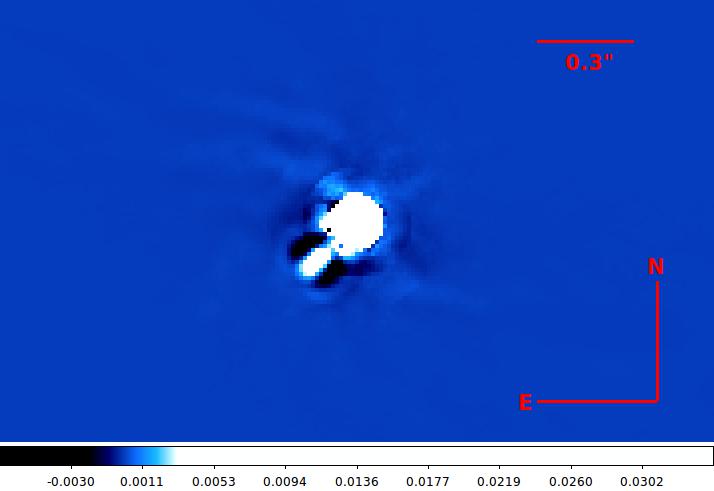
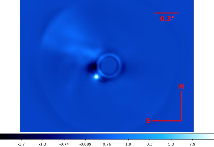
Figure 1: Final images for R CrA system obtained from the best SPHERE dataset taken on 2018-06-19 (chosen because it is the best quality observation epoch). Both of them are obtained from a median of the images at all the wavelengths covered by the two instruments. Left: Final image obtained with IRDIS. Right: Final images obtained with IFS. Both images have flux scales in such a way to make the presence of the companion clear. In both images there is however hints of the presence of the jet-like structure described in Section 4.

A companion is found in the final images of all the epochs of observations. In Figure 1 we show the final images that we obtained from the 2018-06-19 data that, as explained in Section 2, allowed to obtain much deeper images. The scales used in these images have been chosen to better visualize the companion but it is however apparent the presence of extended structures that we will discuss much in detail in Section 4.2. The companion is less visible in the data taken on 2016-08-10, maybe due to the shorter wavelength set up chosen for this observation coupled with a very red spectrum of the source as we will show in Section 4.1.

In Table 2 we list the relative astrometric values for the companion while in Figure 2 we display the relative positions of the companion with respect to the star, compared to the position that it would have had if it were a stationary background object, demonstrating that it is actually comoving with the star. We interpret the variations in the companion separation and position angle as evidences of its orbital motion. To further confirm this, we have to consider that the scatter in velocity for CrA members is of the order of 1-2 km/s while the scatter in velocity between the companion and the central star is between 5 and 10 km/s. This is an other hint that we are actually observing the orbital motion of the companion around the central star.

Two main problems affect the extraction of the photometry. Both of them are linked to the characteristics of the star itself. The first one is due to the large difference in magnitude according to the considered spectral band. Given the high brightness of the star in the H and K band, we had to use the strongest neutral density filter (ND3.5) for the observation of the off-axis PSF to avoid saturation of the star (see Section 2). In this way, however, the star was no longer visible in the IFS Y and J band channels. This of course does not allow a proper flux calibration at these wavelengths. Moreover, the star is strongly variable and for this reason it is difficult to define the absolute magnitude of the companion starting from the contrast (when possible to retrieve). To overcome these problems and to obtain a reliable spectrum of the companion, we have then compared the PSF of R CrA at each wavelength obtained from the observation of 2018-06-19, when available, to the PSFs of other stars taken during the same night in similar conditions. They are HIP 63847 and HIP 70833 that are not known as variable stars. The results are similar for both stars and they allow to define a value for H of $6.95\pm 0.29$ mag and for K of $4.63\pm 0.32$ mag for R CrA at the epoch of our observation. Also, it was possible to put upper limits to the Y and J magnitudes: Y$>$10.92 mag and J$>$8.36 mag. The comparison of these values with those given in literature (see Section 3) put our observation at (or very near to) the minimum of the star brightness variability. Given the comparable results obtained previously we used as reference the PSF of only HIP 63847 to be able to extract the spectrum in flux for R CrA B shown in Figure 7. As a first step we calculated the spectrum in contrast with respect to the reference star introducing a negative simulated planet at the companion position and run our speckle subtraction procedure adjusting its flux in such a way to minimize the standard deviation in a small region around the companion position. We apply this procedure both using an ADI and a PCA-based data reduction and we obtained comparable results. The contrast spectrum was then converted to flux by multiplying it by a flux-calibrated BT-NEXTGEN (Allard et al. 2012) synthetic spectrum for HIP 63847 adopting $T_{eff}$=5300 K, $\log{g}$=-0.5 and [M/H]=-0.5 that gives the best fit to the SED of the star according to the VOSA tool (Bayo et al. 2008).

Table 2: Astrometric results obtained for R CrA B.

Date	$\Delta$RA (′′)	$\Delta$Dec (′′)	$\rho$ (′′)	PA
2015-06-10	0.098$\pm$0.004	-0.121$\pm$0.004	0.156$\pm$0.004	141.0$\pm$0.2
2016-08-10	0.117$\pm$0.004	-0.140$\pm$0.004	0.182$\pm$0.004	140.0$\pm$0.2
2018-06-19	0.134$\pm$0.001	-0.129$\pm$0.001	0.184$\pm$0.001	134.2$\pm$0.2
2018-08-16	0.132$\pm$0.004	-0.128$\pm$0.004	0.184$\pm$0.004	134.0$\pm$0.2

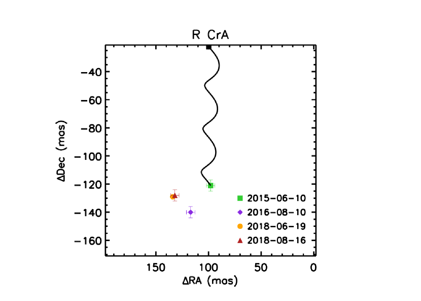
Figure 2: Relative astrometric position of R CrA B with respect to the host star at four different epochs. In black it is shown the path the object would have followed in the three years between the first and the fourth epochs. The black square corresponds to the expected position for the companion at the epoch of the third observation if it were a stationary background object.

4.2 Jet-like structure and circumstellar environment

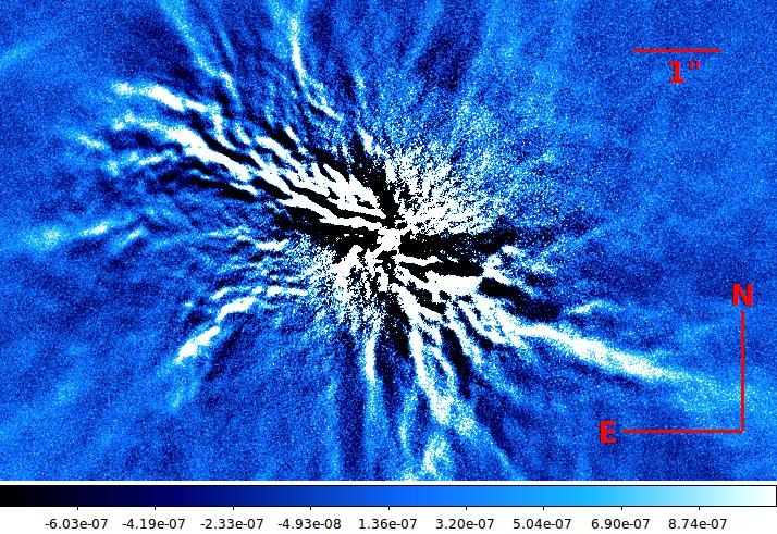
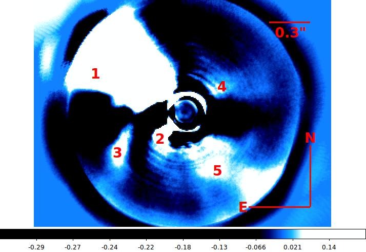
Figure 3: Final images obtained for IRDIS using SpeCal TLOCI (Left) and IFS using PCA with 10 principal components (Right) scaled in such a way to enlight the presence of extended structures. In the IFS image we tag with 1 a jet-like structure, with 2 the position of the companion, with 3 and 4 two faint structures that could be part of the disk and with 5 a fainter counter-jet.

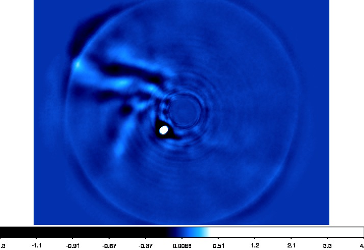
Figure 4: Final IFS image after the subtraction of PCA 100 principal components aimed to highlight the presence of different substructure into the jet-like structure North-East from R CrA. Scale and orientation are the same as those on the right panel of Figure 3.

The environment around R CrA is very rich of different extended structures as it is shown in Figure 3 where we display the final images obtained with IRDIS and IFS with a scale thought to highlight the presence of extended structures. The most striking of them is the jet-like structure North-East from the star that is tagged with 1 in the IFS image (right panel of Figure 3). The same structure is also clearly visible in the IRDIS image (left panel of Figure 3) up to a separation of 3.5^′′ corresponding to a projected separation of more than 535 au. The position angle of median axis of the jet-like structure, calculated using the IFS image, is of $57.8\pm 8.4^{\circ}$. The IRDIS image allows to define an aperture of $\pm 14^{\circ}$ at the maximum separation at which it is visible. However, from the IFS image obtained subtracting 100 principal PCA components displayed in Figure 4, it is clear that the jet-like structure consists of at least two separated structures with position angles of $66.1^{\circ}$ and $49.4^{\circ}$ respectively. This is not an artefact of the differential imaging because the two structures are clearly visible also on images where no differential imaging was applied. The structure and the nature of this jet-like structure will be studied in more detail in a dedicated paper (Rigliaco et al., in prep.). A fainter counter-jet-like structure is also visible both in the IRDIS and the IFS images at an angle of about $180^{\circ}$ with respect to the jet-like structure described above and it is tagged with 5 in the IFS image in Figure 3. Another curved structure is visible South-East of the star and apparently it starts from the base of the jet-like structure and not from the star itself. It is tagged with 3 in the IFS image in Figure 3 but it is even more clearly visible in Figure 4. Its approximated position angle is $103.5^{\circ}$ and it could be part of an external disk of which could also be part the very faint structure tagged 4 North-West to the star with a position angle of $305.9^{\circ}\pm 9.0^{\circ}$ at $\sim 180^{\circ}$ from the position of the companion (tagged 2 in Figure 3).

4.3 Results from SINFONI data

The companion was retrieved also in the SINFONI data as shown in the median image of the final datacube obtained applying the ADI method that is displayed in Figure 5. From the final datacube, applying aperture photometry at each single wavelength image, we were then able to extract the spectrum for the companion that was then corrected for telluric absorption using data from a B2 standard star (HD 203617) observed during the same night and at a similar airmass. The extracted SINFONI spectrum is very noisy at shorter and longer wavelengths and, for this reason, the reduction of the telluric absorption was not effective at those wavelengths and we decided to retain only wavelengths between 1.50 and 1.75 $\mu$m remaining with 1282 wavelengths that were then used to perform the cross-correlation procedure described in Section 5.3.

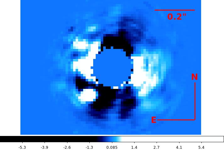
Figure 5: R CrA image resulting from the median of the final SINFONI datacube obtained applying the ADI technique.

5 Discussion

5.1 Characterization of the companion through evolutionary models

The very strong and variable absorption of the CrA region does not allow to blindly use the determinations of the absorption listed in Section 3. To overcome this problem we have exploited the isochrones of the BT-Settl models (Allard 2014). In Figure 6 we show the 1 and 2 Myr isochrones for J vs. J-H compared with the value of J-H=$2.18\pm 0.11$ (red vertical line) calculated for the companion of R CrA from the extracted apparent magnitudes that are listed in the second column of Table 3. As a first step we calculated the value of the reddening E(J-H) taking as reference the median value of J-H for the 1 Myr isochrone in the region with 6$<$J$<$9 where the value of J-H is almost constant. We then calculated the corresponding value of $A_{J}$ using the formula from Cardelli et al. (1989). With this value and applying the appropriate correction for the distance modulus we can retrieve the absolute magnitude in the J band that, through the use of the BT-Settl models, allow to estimate the mass of the companion. Using the BT-Settl models we can then obtain the absolute magnitude also for the H band and from this calculate an updated value for J-H and for E(J-H) comparing the latter to the original value for the companion. We then checked if the initial value of E(J-H) corresponds to the new value that we obtain from the model. We iterated the steps described above until the difference between the input and the output values for E(J-H) is less than 0.01 mag. Once we have obtained the final values for $A_{J}$ and for the absolute magnitude in the J band, we retrieved the same values also for all the other spectral bands. These results are listed in column four and five of Table 3.

Moreover, the absolute magnitudes listed in Table 3 allow to define some of the main physical characteristics of R CrA B through the use of the BT-Settl models. We obtained for the mass a value of $0.29\pm 0.08$ M_⊙, $T_{eff}$=$3270\pm 175$ K, $\log{g}$=$3.45\pm 0.06$ and finally a radius of $16.7\pm 4.2$ R_Jup. To evaluate the errors in these results we took into account the uncertainties on the distance, on the age and on the magnitudes of the host star. According to Pecaut & Mamajek (2013) the value of $T_{eff}$ that we found would correspond to a spectral type of M3-M3.5. The relatively low surface gravity found for the companion, coupled to the large radius, are hints for a not fully completed gravitational collapse as expected for such young objects.

The value of $A_{J}$ was used to derive an estimate of $A_{V}$=15.89 and, assuming a value of $R_{V}$=4.7, we obtained a E(B-V)=3.38. These values were then used to correct the spectrum obtained with the procedure described in Section 4.1 using the IDL ccm_unred routine based on the Cardelli et al. (1989) formula. While the uncorrected spectrum is very red, after the correction we remain with a much bluer spectrum typical of a stellar object.

Table 3: Photometric results obtained for R CrA B. The second column lists its apparent magnitudes before the correction for the extinction, the third column the differences in magnitudes with respect to the central star, the fourth column lists the values of the estimated extinction and finally the fifth column presents its absolute magnitudes after the correction for the extinction.

Spectral band	App. mag	$\Delta$Mag	$A_{\lambda}$	Dered abs. mag.
Y	$16.45\pm 0.05$	$5.53\pm 0.19$	$5.83\pm 0.32$	$4.70\pm 0.27$
J	$14.60\pm 0.08$	$6.24\pm 0.74$	$4.48\pm 0.26$	$4.20\pm 0.26$
H	$12.42\pm 0.03$	$5.47\pm 0.32$	$3.01\pm 0.38$	$3.49\pm 0.35$
K1	$10.63\pm 0.01$	$6.00\pm 0.33$	$1.36\pm 0.30$	$3.35\pm 0.29$
K2	$10.27\pm 0.01$	$5.64\pm 0.33$	$1.18\pm 0.28$	$3.17\pm 0.27$

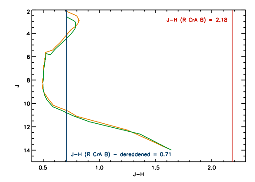
Figure 6: Isochrones J vs J-H in the case of 1 Myr (orange line) and 2 Myr (green line). The red vertical line represents the J-H value calculated for R CrA B.

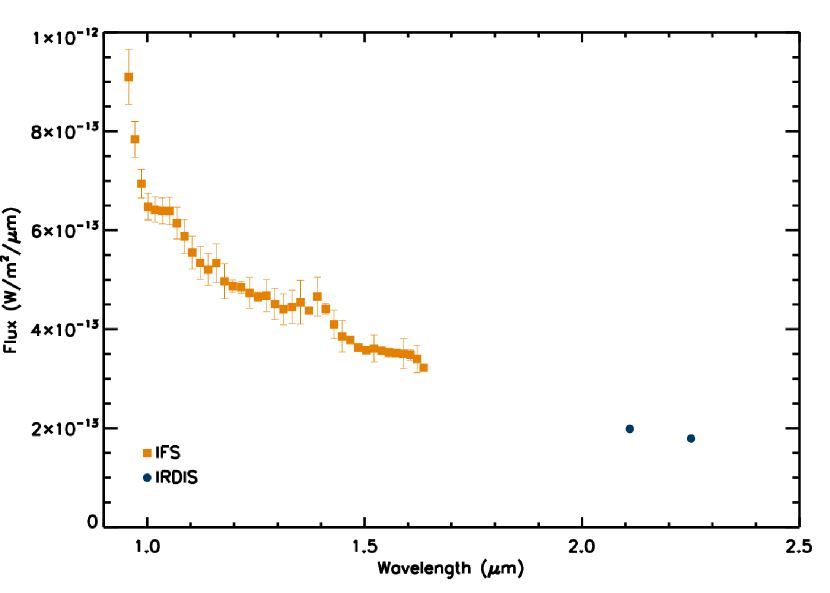
Figure 7: Final spectrum extracted for R CrA B from SPHERE data after applying the correction for the extinction. The orange squares are measures obtained with IFS while the blue circles are obtained with IRDIS. In this last case the error bars are smaller than the symbol size.

5.2 Fitting with template spectra and atmospheric models

To further characterize the companion we have tried to fit its extracted spectrum with libraries of template spectra with the aim to define its spectral type. To this aim we have used the library of field BDs spectra taken from the Spex Prism spectral Libraries (Burgasser 2014) and the library of spectra taken from Allers & Liu (2013). The procedure is similar to those adopted in Mesa et al. (2016), Mesa et al. (2018) and Ligi et al. (2018). For the fit we did not use the three spectral points at shorter wavelengths that are anomalously high as can be seen in Figure 7. This is probably due to a contamination arising from the particular configuration of the IFS raw data (see e.g. Claudi et al. 2008). In these data the faint blue ends of the R CrA B spectrum in one spaxel are adjacent to the very bright red ends of the spectrum on a near spaxel. This results in some light from the bright red pixel leaking toward the faint blue pixels. The final results for the fit procedure are shown in Figure 8 and are compatible with an early-M spectral type for the companion.

We have also tried to fit the extracted spectra with a set of BT-Settl and BT-NextGen atmospheric models (Allard et al. 1997; Allard 2014) with a grid covering $T_{eff}$ between 900 and 4000 K with a step of 100 K and a $\log{g}$ ranging between 2.5 and 5.5 dex, with a step of 0.5. All the models were for a solar metallicity. The results of this procedure are displayed in Figure 9. From these results it is difficult to draw a conclusion given that a lot of different models fit well with our results. However, the results are compatible with a high $T_{eff}$ in the range between 3500 and 4000 K. Also, they seem to favour high surface gravity models. These results are in contrast with what we obtained in Section 5.1 where the value of $T_{eff}$ was slightly lower and moreover we were favouring a low surface gravity result.

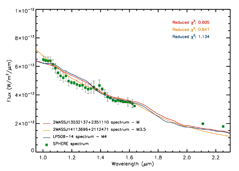
Figure 8: Comparison of the R CrA B spectrum obtained from SPHERE (green squares) with three of the best fit template spectra.

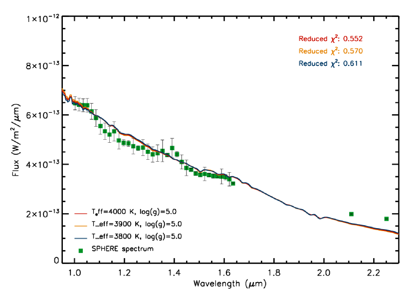
Figure 9: Comparison of the R CrA B spectrum obtained from SPHERE (green squares) with three of the best fit BT-Settl atmospheric models.

5.3 Characterization of the companion through SINFONI data

The spectrum extracted from the SINFONI data was used to obtain a further spectral classification of the object by comparing it with a library of template spectra of K and M stars taken from the IRTF library (Cushing et al. 2005; Rayner et al. 2009). The comparison was done through the spectral lines and, to avoid the final result to be influenced by the slope of the spectra strongly dependent from the very uncertain value of the extinction, we have divided each spectrum that we used for a smoothed version of itself to eliminate any slope. The smoothing was done with the standard SMOOTH IDL procedure using a smoothing window of 100. The spectra were then compared using the C_CORRELATE IDL routine trying to maximize the cross-correlation index between them. Moreover, to explore the possible shift of the spectra due to the radial velocity of R CrA, this procedure was executed shifting the template spectra of arbitrary wavelength values. In any case, we always found that the highest cross-correlation indices were obtained for shifts very near to zero concluding that the radial velocity of R CrAhave to be very close to 0. The same procedure was then repeated using a library of young stars spectra obtained by Manara et al. (2013) and Manara et al. (2017) from X-SHOOTER data. In Figure 10 we display the values of the cross-correlation index as a function of the spectral type that we obtain from the procedure described above showing in orange the values obtained from the IRTF data and in green the values obtained from the X-SHOOTER data. The evolution of the cross-correlation index is very similar in both cases. The maximum values are obtained for spectral types between M0 and M1.5 where the value of the index is almost stable. On the low-mass side the values of the indices diminish with a steep slope while a shallower slope is found on the side of the K-stars. In Figure 11 we display the normalized spectrum of R CrA B together with those of some of the best fit spectra from the IRTF library. The fit of the spectral lines between the compared spectra is good with values of the cross-correlation index between 0.46 and 0.48 for the best fit spectra. In the image we have tagged some of the most prominent lines in the spectra identifying lines from Mg I, Fe I, Si I and Al I. An evident line in the R CrA B spectrum is also present at 1.67 $\mu$m but it is not present in the template spectra. It is probably a telluric line that has not been completely deleted by the subtraction of the telluric spectrum standard and for this reason we have tagged it with ’T’ in Figure 11. Using the spectral classification obtained from this method, we obtain for R CrA B a $T_{eff}$ between 3650 and 3870 K that, from the isochrones for pre-main sequence stars by Baraffe et al. (2015), corresponds to a mass between 0.47 and 0.55 M_⊙.

We also used the H lines in the spectral region observed with SINFONI to search for any evidence of accretion. However, the upper limit to the equivalent width (EW), obtained from the median of H lines in this region, is of 0.05 nm. As a comparison we can consider the Orion low mass stars considered in Rigliaco et al. (2012) that have an EW of $\sim$0.1 nm. We can then conclude that there is no evidence of accretion for R CrA B even if we have to consider that accretion for this object is very probably variable while we have obtained a spectrum in just one epoch.

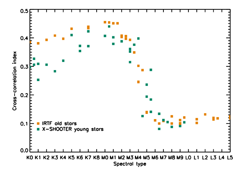
Figure 10: Values of the cross-correlation index between the SINFONI spectrum of R CrA B and template spectra from the IRTF library (orange squares) and X-SHOOTER young stars (green squares) vs. the spectral type of the template spectra.

Figure 11: Comparison of the R CrA B (black line) spectrum with those of some of the best fit spectra from the spectral libraries.

5.4 Orbital parameters

Using the astrometric data listed in Table 2 we have performed a Monte Carlo simulation to constrain the orbital parameters using the Thiele-Innes formalism (Binnendijk 1960) as described in Desidera et al. (2011), Zurlo et al. (2013) and Zurlo et al. (2018) and adopting the convention by Heintz (2000). The simulation generates by $5\times 10^{7}$ random orbital elements and rejects all the central orbits that do not fit the astrometric data. Given that the mass of the star is poorly constrained through previous studies, we have also decided to include it between the varying parameters of our simulation considering a very large mass range of 2-30 M_⊙. We also assumed a large variation of the mass of the companion between 1 and 1000 M_Jup. The simulation found 144249 orbits consistent with the observational data. The results of this procedure for the main parameters are shown in Figure 12. The simulation clearly prefers a low mass for the whole system, an eccentricity of $\sim$0.4, a semi-major axis of 27-28 au and an inclination of $\sim 70^{\circ}$. However, we are not able to obtain a good value for the companion mass given that its distribution is quite uniform and for the period even if in this case periods of less than 30 years are clearly excluded and we have a very smoothed peak at about 65-70 years. The availability of long term RV-data could help in constraining the system mass-ratio. Unfortunately, we did not find any data of this type for R CrA.

Figure 12: Distribution histograms obtained from the Monte Carlo simulation described in Section 5.4 for the total mass of the system in solar masses (upper left panel), the ellipticity (upper right panel), the semi-major axis in au (center left panel), the companion mass in M_Jup(center right panel), the inclination of the orbit (bottom left panel) and the period in years bottom right panel).

5.5 Mass limits around R CrA

With the aim to estimate the mass limits for other possible objects around R CrA we have calculated the brightness contrast following the method devised in Mesa et al. (2015). In this case, however, to overcome the problems arising from the variability of R CrA, we have used as reference the star HIP 63847 following the same procedure used to obtain the results in Section 4.1. We then obtained the contrast in absolute magnitude and we have corrected it for the extinction that we have calculated for the companion in Table 3. While these values are not necessarily valid for all the region around R CrA, we have used them to give an estimate of the effective contrast. This result was then used in association with the AMES-Dusty models to evaluate the mass limits for other objects around the star. The results of this procedure are displayed in Figure 13. Due to the much larger extinction at shorter wavelengths, IFS is in this case less effective in finding low mass companions, hence we can use IRDIS to set these limits. At separations from the star less than 100 au, we are able to obtain mass limits variable, according to the separation, between 6 and 2.5 M_Jup while at larger separations we can reach an almost stable mass limit of the order of 1.5 M_Jup.

Figure 13: Plot of the mass limits expressed in M_Jup vs. the separation expressed in au for possible objects around R CrA. The IFS limits are given by the orange line while the IRDIS limits are given by the green line.

6 Conclusions

In this paper we report the results from the SPHERE multi-epoch observations of the R CrAsystem. The central star is a very young ($\sim$1 Myr) HAeBe object with a strong reddening due to the presence of circumstellar material. The star is strongly variable on period of $\sim$66 days and, moreover, it has strong differences in magnitude between different spectral bands. These facts make difficult a proper photometric characterization of companion objects.

A companion was found around the star and, thanks to the astrometric measurements taken during the four observing epochs, we were able to confirm that it is gravitationally bound to the star. Also, we were able to extract a spectrum of the companion. After correction for extinction in the direction of the companion and through the comparison with the BT-Settl evolutionary models we were able to infer for the companion a mass of 0.29$\pm$0.08 M_⊙. Hence, the companion is an early M spectral type star deeply embedded in its dust envelope. This case is then very similar to that of the two companions of T Tau, T Tau S a and T Tau S b (Dyck et al. 1982; Kasper et al. 2016). An alternative explanation of the strong extinction in the direction of the companion is that it could be due to the presence of an external disk seen at very large inclination. Despite the fact that we have found some hints of the presence of this external disk, we are not able at the moment to disentangle between the two explanations of the large extinction in the direction of the companion. The spectral classification of the companion is further confirmed comparing template spectra to the companion spectrum obtained using SINFONI. The results obtained with the latter instrument provide a slightly higher value both for the mass (0.47-0.55 M_⊙) and for $T_{eff}$ (3650-3870 K) than what obtained from the SPHERE data. This discrepancy could be due to the fact that the extinction value determined from SPHERE data is slightly underestimated obtaining in this latter case a value of $A_{J}$=5.00 mag. Moreover, given that the classification through the SINFONI data relies on spectral lines that are not affected by the extinction, we believe that the latter are a more reliable estimate of the companion mass. The higher temperature derived from the spectral lines through SINFONI data might be due to the presence of a hotter region on the stellar surface related to accretion. In addition, we notice that no emission line was detected in our SINFONI spectrum, although several lines in the Brackett series are included in the observed spectral range with an upper limit to the EW of 0.05 nm. It is then worth to notice that, using for the star the distance of 94.9 pc derived from the Gaia parallax, we would obtain from the comparison with the BT-Settl evolutionary models a mass of the order of $0.14\pm 0.03$ M_⊙ corresponding to a spectral type of M5-M6. This would be even more in contrast with the mass determination obtained from the SINFONI spectrum of the companion that is not depending from the distance of the star. This gives even more strength to our estimate of the distance of the system made in Section 3.

The position of the stellar companion probably in a gap in the disk around the primary star of the system could make this object a candidate for formation through disk instability as proposed e.g. by Forgan et al. (2016) for massive young protostars with a large disc-star mass ratio. A similar object has been recently discovered through ALMA observations around the young stellar object G11.92-0.61 MM1 (Ilee et al. 2018). In any case, to confirm this possibility we will need more precise informations both about the physical characteristics (e.g. its mass that is still poorly defined) of the primary star of the system and on the effective location of the companion into the gap of the disk for which we have at the moment just non-conclusive hints.

Aside to the presence of the companion, the environment around R CrA is further enriched by the presence of a number of extended structures. The most notable of them is surely the bright jet-like structure North-East of the star. Our images highlight moreover that this jet-like structure is itself formed by at least two substructures. A less bright counter-jet-like structure on the opposite side of the star is also visible together with some arc-like structures that could be part of an external disk. Instead, in our images it is not possible to image the inner disk that the star is known to host. We will discuss the nature and the origin of the jet-like structure and of all the other extended structures in this system in a following dedicated paper.