Velocity-determined anisotropic behaviors of RKKY interaction in 8-Pmmn borophene

Abstract

As a new two-dimensional Dirac material, 8-Pmmn borophene hosts novel anisotropic and tilted massless Dirac fermions (MDFs) and has attracted increasing interest. However, the potential application of 8-Pmmn borophene in spin fields has not been explored. Here, we study the long-range RKKY interaction mediated by anisotropic and tilted MDFs in magnetically-doped 8-Pmmn borophene. To this aim, we carefully analyze the unique real-space propagation of anisotropic and tilted MDFs with noncolinear momenta and group velocities. As a result, we analytically demonstrate the anisotropic behaviors of long-range RKKY interaction, which have no dependence on the Fermi level but are velocity-determined, i.e., the anisotropy degrees of oscillation period and envelop amplitude are determined by the anisotropic and tilted velocities. The velocity-determined RKKY interaction favors to fully determine the characteristic velocities of anisotropic and tilted MDFs through its measurement, and has high tunability by engineering velocities shedding light on the application of 8-Pmmn borophene in spin fields.

I Introduction

The charge and spin are two intrinsic ingredients of the electron, and the success of electronics based on the charge transport lures people to develop the spin-related applications Žutić et al. (2004); Fert (2008). However, a lot of solid-state materials are nonmagnetic and/or do not show its spin properties, then hinder their applications in spin fields. One way to surmount the obstacle is through the doping of nonmagnetic materials with magnetic impurity atoms Power and Ferreira (2013). The itinerant carriers of host materials can help to couple the magnetic impurities indirectly, i.e., the Rudermann-Kittel-Kasuya-Yosida (RKKY) interaction Ruderman and Kittel (1954); Kasuya (1956); Yosida (1957). The RKKY interaction is an important mechanism underlying rich magnetic phases in diluted magnetic systems Jungwirth et al. (2006) and giant magneto-resistance devices Fert (2008), and has potential applications in spintronics Wolf et al. (2001); Žutić et al. (2004); MacDonald et al. (2005), and scalable quantum computation Loss and DiVincenzo (1998); Trifunovic et al. (2012), as the RKKY interaction enables long-range coupling of distant spinsPiermarocchi et al. (2002); Craig et al. (2004); Rikitake and Imamura (2005); Friesen et al. (2007); Srinivasa et al. (2015).

The importance of RKKY interaction makes its research to closely accompany the advent and development of new materials. In recent years, the RKKY interaction has been widely studied in various materials such as graphene Saremi (2007); Brey et al. (2007); Hwang and Das Sarma (2008); Sherafati and Satpathy (2011); Kogan (2011), monolayer transition-metal dichalcogenides Parhizgar et al. (2013a); Hatami et al. (2014); Mastrogiuseppe et al. (2014); Ávalos-Ovando et al. (2016a, b, 2019) topological insulators Liu et al. (2009); Zhu et al. (2011); Abanin and Pesin (2011); Hsu et al. (2017, 2018); Zhang et al. (2018), siliceneZare et al. (2016); Duan et al. (2018), phosphoreneDuan et al. (2017); Zare and Sadeghi (2018); Islam et al. (2018), layered structures Masrour et al. (2016); Jabar and Masrour (2017, 2018); Jabar et al. (2019) and Dirac and Weyl semimetals Hosseini and Askari (2015); Chang et al. (2015); Mastrogiuseppe et al. (2016). Among these studies, the RKKY interaction mediated by massless Dirac fermions (MDFs) has attracted a lot of interest, which exhibits many new behaviors and brings about potential opportunities of nonmagnetic Dirac materials for spin applications. However, previous studies are mainly limited to the Dirac materials with isotropic MDFs, this leaves the influence of novel MDFs on the RKKY interaction unexplored.

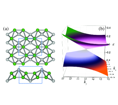
Figure 1: (a) Crystal structure of 8-Pmmn borophene from top view (upper panel) and side view (bottom panel). The ridge boron atom (green) and the inner boron atom (gray) are nonequivalent. In each unit cell, there are eight atoms delimited by the dashed blue rectangle. (b) Anisotropic and tilted Dirac cone in 8-Pmmn borophene.

The 8-Pmmn borophene with the crystal structure of Fig. 1(a) is one kind of two-dimensional Dirac material, in which the novel MDFs are anisotropic and tilted as shown by Fig. 1(b) in contrast to those isotropic ones in the well-known graphene. Recently, since its seminal prediction Zhou et al. (2014), wide theoretical efforts have been paid to calculate the unprecedented electronic properties Lopez-Bezanilla and Littlewood (2016); Zabolotskiy and Lozovik (2016); Nakhaee et al. (2018a, b) and to construct the effective low-energy continuum Hamiltonian Zabolotskiy and Lozovik (2016); Nakhaee et al. (2018a) which has been used to study the plasmon dispersion and screening properties Sadhukhan and Agarwal (2017), the optical conductivity Verma et al. (2017), Weiss oscillations Islam and Jayannavar (2017), and Metal-insulator transition induced by strong electromagnetic radiation Champo and Naumis (2019). The rapid experimental advances of various borophene monolayers Mannix et al. (2015); Feng et al. (2016, 2017) further boost wider research interest on 8-Pmmn borophene. The anisotropic exchange coupling and the magnetic anisotropy are very crucial to spin applicationsŽutić et al. (2004); Jungwirth et al. (2006); Shi and Jiang (2018); Shi et al. (2018); Zou et al. (2018), so our interest is to examine the anisotropic features of RKKY interaction due to the novel MDFs.. Here, we study the RKKY interaction mediated by the anisotropic and tilted MDFs by using the effective model of 8-Pmmn borophene. In the long range, we analytically derive the Green’s function (GF) of anisotropic and tilted MDFs to show the unique real-space propagation properties, and then their mediation to RKKY interaction whose oscillation period and envelop amplitude are both anisotropic and determined by the velocities, i.e., velocity-determined RKKY interaction. As a result, our theoretical study show the potential of velocity-determined RKKY interaction in the characterization of characteristic velocities of anisotropic tilted MDFs and the application of 8-Pmmn borophene for spin fields.

This paper is organized as follows. In Sec. II, we start from the intrinsic electronic properties of 8-Pmmn borophene, present the general expression of RKKY interaction, and reveal the analytical behaviors of the real-space GF including the symmetry properties, the classical trajectories and the explicit analytical expression. Then in Sec. III, we perform exact numerical calculations to show the typical features of velocity-determined RKKY interaction. Most importantly, the analytical expression for RKKY is derived and is used to understand the velocity-determined RKKY interaction. Finally, we summarize this study in Sec. IV.

II Theoretical formalism

In 8-Pmmn borophene, the effective Hamiltonian of anisotropic and tilted MDFs near one Dirac cone is Zabolotskiy and Lozovik (2016); Islam and Jayannavar (2017)

$$\hat{H}_{0}=(v_{x}\sigma_{x}\hat{p}_{x}+v_{y}\sigma_{y}\hat{p}_{y}+v_{t}\sigma_{0}\hat{p}_{y}),$$ (1)

where $\hat{p}_{x,y}$ are the momentum operators, $\sigma_{x,y}$ are $2\times 2$ Pauli matrices, and $\sigma_{0}$ is the $2\times 2$ identity matrix. The anisotropic velocities are $v_{x}=0.86v_{F}$, $v_{y}=0.69v_{F}$, and $v_{t}=0.32v_{F}$ with $v_{F}=10^{6}$ m/s. In this study, we set $\hbar=v_{F}\equiv 1$ to favor our dimensionless derivation and calculations since they can define the length unit $l_{0}$ and the energy unit $\varepsilon_{0}$ through $\hbar v_{F}=l_{0}\varepsilon_{0}$, e.g., $\varepsilon_{0}=0.66$ eV when $l_{0}=1$ nm. To solve the Schödinger equation $\hat{H}_{0}\psi=\varepsilon\psi$, the energy dispersion [see Fig. 1(b)] and the corresponding wave functions are, respectively,

$$\varepsilon_{\lambda,\mathbf{k}}=v_{t}k_{y}+\lambda\sqrt{v_{x}^{2}k_{x}^{2}+v_{y}^{2}k_{y}^{2}},$$ (2)

and

$$\psi_{\lambda,\mathbf{k}}(\mathbf{r})=e^{i\mathbf{k}\cdot\mathbf{r}}|u_{\lambda}(k_{x},k_{y})\rangle$$ (3)

with

$$|u_{\lambda}(k_{x},k_{y})\rangle\equiv\frac{1}{\sqrt{2}}\begin{bmatrix}1\\ \frac{\left(v_{x}k_{x}+iv_{y}k_{y}\right)}{\varepsilon_{\lambda,\mathbf{k}}-v_{t}k_{y}}\end{bmatrix}.$$

Here, $\lambda=\pm$ denotes the conduction (valence) band, $\mathbf{k=}(k_{x},k_{y})$ and $\mathbf{r=}(x,y)$ are, respectively, the momentum and position vectors, and $|u_{\lambda}(k_{x},k_{y})\rangle$ is the spinor part of the wave function.

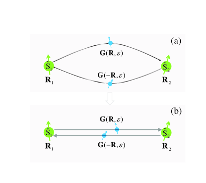
Figure 2: Schematic diagram of RKKY interaction of two localized spins $\hat{\mathbf{S}}_{1,2}$ at $\mathbf{R}_{1,2}$ mediated by the propagation Green’s functions $\mathbf{G}(\mathbf{R,}\varepsilon)$ and $\mathbf{G}(-\mathbf{R},\varepsilon)$ of itinerant carriers between them. Generally, all quantum states below the Fermi level $\varepsilon_{F}$ (see Eq. 4) contribute to the Green’s functions as shown by the curved dotted lines in (a), and then the RKKY interaction. However, at large distances, the Green’s functions are dominated by the states with group velocities parallel to $\mathbf{R}$ (i.e., the classical trajectories as shown by the straight solid lines in (b)), and then RKKY interaction is determined by the limited momentum states on the Fermi surface (see Eq. 27).

II.1 Expression for the RKKY interaction

In the uniform 8-Pmmn borophene, as shown by Fig. 2(a), for two local spins $\hat{\mathbf{S}}_{1,2}$ at $\mathbf{R}_{1,2}$ coupled to the carrier spin density $\hat{\mathbf{s}}(\mathbf{x})=\hat{\mathbf{s}}\delta(\hat{\mathbf{r}}-\mathbf{x})$ via the s-d exchange interaction $-J_{0}\hat{\mathbf{S}}_{1}\cdot\hat{\mathbf{s}}(\mathbf{R}_{1})-J_{0}\hat{\mathbf{S}}_{2}\cdot\hat{\mathbf{s}}(\mathbf{R}_{2})$, the carrier-mediated RKKY interaction assumes the isotropic Heisenberg form due to the absence of spin-orbit coupling, i.e., $\hat{H}_{\text{RKKY}}=J_{jj^{\prime}}\mathbf{\hat{S}}_{1}\cdot\mathbf{\hat{S}}_{2}$, where the range function Sherafati and Satpathy (2011); Klinovaja and Loss (2013); Zhang et al. (2017)

$$J_{jj^{\prime}}(\varepsilon_{F},\mathbf{R})=-\frac{J_{0}^{2}}{2\pi}\operatorname{Im}\int_{-\infty}^{\varepsilon_{F}}\digamma_{jj^{\prime}}(\varepsilon,\mathbf{R})d\varepsilon$$ (4)

is determined by the intrinsic real-space GF of carriers, i.e.,

$$\digamma_{jj^{\prime}}(\varepsilon,\mathbf{R})=G_{jj^{\prime}}(\mathbf{R},\varepsilon)G_{j^{\prime}j}(-\mathbf{R},\varepsilon).$$ (5)

Due to the integral forms of Eq. 4 over the energy and of Eq. 7 over the momentum (see the subsequent subsection), all quantum states propagating between $\mathbf{R}_{1}$ and $\mathbf{R}_{2}$ below the Fermi level $\varepsilon_{F}$ contribute to the RKKY interaction as shown by the curved dotted line in Fig. 2(a). In addition, $j,j^{\prime}\in\{1,2\}$ label the orbitals used in the basis for the Hamiltonian of 8-Pmmn borophene. Until now, the respective contribution of different orbitals to form the Dirac states of 8-Pmmn borophene is still in debate Zabolotskiy and Lozovik (2016) and the interaction properties between magnetic impurity and the borons’ orbitals call for further density functional calculations, so we focus on the long-range behaviors of RKKY interaction in our model study.

II.2 Real-space GF

The real-space GF is the key to understand the spatial propagation of carries and their mediation to the RKKY interaction, which is defined by

$$\mathbf{G}(\mathbf{R},\varepsilon)\equiv\langle\mathbf{R}_{2}|(\varepsilon+i0^{+}-\hat{H}_{0})^{-1}|\mathbf{R}_{1}\rangle.$$ (6)

Here, $\mathbf{R=R}_{2}-\mathbf{R}_{1}\$accounts for the translational invariance in uniform system and is the connecting vector for two magnetic impurities, and $\mathbf{G}$ is one $2\times 2$ matrix expressed in the orbital basis instead of the spin basis originating from the spin-degenerate Hamiltonian of 8-Pmmn borophene in the orbital basisZabolotskiy and Lozovik (2016). The real-space GF can be obtained from the Fourier transformation

$$\mathbf{G}(\mathbf{R},\varepsilon)=\frac{1}{4\pi^{2}}{\displaystyle\iint}d^{2}\mathbf{k}e^{i\mathbf{k}\cdot\mathbf{R}}\mathbf{G}(\mathbf{k},\varepsilon),$$ (7)

of the momentum-space GF

$$\mathbf{G}(\mathbf{k},\varepsilon)\equiv[z-H_{0}(\mathbf{k})]^{-1}=-\frac{2(\epsilon-\gamma_{2}k_{y})}{v_{x}}\frac{|u_{\lambda}(k_{x},k_{y})\rangle\langle u_{\lambda}(k_{x},k_{y})|}{(k_{x}-k_{x,+})(k_{x}-k_{x,-})}.$$ (8)

with

$$k_{x,\pm}(k_{y})=\pm\sqrt{(\epsilon-\gamma_{2}k_{y})^{2}-\gamma_{1}^{2}k_{y}^{2}}.$$ (9)

Here, $\gamma_{1}=v_{y}/v_{x}$, $\gamma_{2}=v_{t}/v_{x}$, $\epsilon=z/v_{x}$ with $z=\varepsilon+i0^{+}$, and $\lambda=\mathrm{sgn}(\epsilon)$ conforms to the energy dispersion. In the definition of momentum-space GF, we have used the form of $\hat{H}_{0}$ in the momentum space, i.e., $H_{0}(\mathbf{k})=\langle\mathbf{k}|\hat{H}_{0}|\mathbf{k}\rangle$. To perform the contour integral over $k_{x}$ straightforwardly:

$$\mathbf{G}(\mathbf{R},\varepsilon)=\frac{\mathrm{sgn}(x)}{2\pi}\int dk_{y}e^{i\phi_{s}}\frac{\epsilon-\gamma_{2}k_{y}}{iv_{x}k_{x,s}}|u_{\lambda}(k_{x},k_{y})\rangle\langle u_{\lambda}(k_{x},k_{y})|,$$ (10)

where $s=\mathrm{sgn}(x)\mathrm{sgn}(\epsilon-\gamma_{2}k_{y})$, and $\phi_{s}(k_{y},\mathbf{R})=k_{x,s}x+k_{y}y$ is the propagation phase factor which has an energy dependence but is omitted for conciseness. And noting here, we always adopt $x=0^{+}$ to replace $x=0$ when we consider $\mathbf{R}$ along the $y$-axis. Later, we firstly discuss the symmetry properties of GF, then derive the dominant contributing states (namely, the classical trajectories) to real-space GF and their features, which help us to derive the analytical expression of real-space GF.

II.2.1 Symmetry properties of GF

From the Eq. 10, the symmetry properties of GF can be derived, which determines the RKKY properties. On one hand, we have $G_{11}(\mathbf{R},\varepsilon)=G_{22}(\mathbf{R},\varepsilon)$, this is identical to the case of graphene with isotropic MDFs Sherafati and Satpathy (2011). However, there is no symmetrical relation between $G_{12}(\mathbf{R},\varepsilon)$ and $G_{21}(\mathbf{R},\varepsilon)$ in contrast to $G_{12}(\mathbf{R},\varepsilon)=G_{21}(\mathbf{R},\varepsilon)$ in graphene Zhang et al. (2017). On the other hand, one can arrive at

$$\mathbf{G}(\mathbf{R},-\varepsilon)=-(\mathbf{G}^{\ast}(\mathbf{R},\varepsilon))^{\text{T}}.$$ (11)

Here, T denotes the transpose operation of a matrix. Eq. 11 is also applicable to isotropic MDFs in graphene as expected from the electron-hole symmetry Zhang et al. (2017), so its origin can be seen as a generalized electron-hole symmetry for anisotropic and tilted MDFs. The symmetry properties is beneficial to the discussions of the RKKY interaction and reduces the numerical calculations as shown in the next section, e.g., our focus can be mainly on the electron-doped case by using Eq. 11.

II.2.2 Classical trajectory: traveling nature and group velocity

The integral form of Eq. 10 over $k_{y}$ shows that in general all momentum states should contribute together to the real-space GF. For convenience, we can separate these momentum states into two classes: traveling states and evanescent states. For the conductance (valence) band with $\lambda=+$ ($\lambda=-$), we have traveling states with $\gamma_{2}k_{y}<\epsilon$ ($\gamma_{2}k_{y}>\epsilon$) and evanescent states with $\gamma_{2}k_{y}>\epsilon$ ($\gamma_{2}k_{y}<\epsilon$). To identify the dominant contributing states to GF, we use the saddle point approximation. According to the saddle point approximation Roth et al. (1966); Liu et al. (2012); Power and Ferreira (2011); Lounis et al. (2011), the dominant contribution to Eq. 10 is the classical trajectory from $\mathbf{R}_{1}$ to $\mathbf{R}_{2}$, which is determined by the first order derivative of propagation phase factor $\phi_{s}$:

$$\frac{\partial\phi_{s}}{\partial k_{y}}=0.$$ (12)

Eq. 12 leads to the identity:

$$\frac{\gamma_{2}(\epsilon-k_{y,s}^{c}\gamma_{2})+\gamma_{1}^{2}k_{y,s}^{c}}{k_{x,s}^{c}}=\tan\theta,$$ (13)

with $\tan\theta=y/x$ and $\theta$ being the azimuthal angle of $\mathbf{R}$ elative to the $x$ axis. Eq. 13 can be rewritten as a quadratic equation with one unknown:

$$(\allowbreak\gamma_{1}^{2}-\gamma_{2}^{2})(k_{y,s}^{c})^{2}+\allowbreak 2\epsilon\gamma_{2}k_{y,s}^{c}+\frac{\epsilon^{2}\left(\gamma_{2}^{2}-\tan^{2}\theta\right)\allowbreak}{\gamma_{1}^{2}-\gamma_{2}^{2}+\tan^{2}\theta}=0.$$ (14)

Once $k_{y,s}^{c}$ are derived, one can obtain $k_{x,s}^{c}=k_{x,s}(k_{y,s}^{c})$ for the classical trajectory. In other words, the classical trajectory has the momentum $\mathbf{k}_{s}^{c}=(k_{x,s}^{c},k_{y,s}^{c})$, in which the components have explicit analytical expressions:

$$k_{x,s}^{c} =\frac{s|\epsilon|\gamma_{1}}{\sqrt{\gamma_{1}^{2}-\gamma_{2}^{2}+\tan^{2}\theta}},$$ (15a)

$$k_{y,s}^{c} =-\frac{1}{\gamma_{1}^{2}-\gamma_{2}^{2}}(\epsilon\gamma_{2}-\frac{s|\epsilon|\gamma_{1}\tan\theta}{\sqrt{\gamma_{1}^{2}-\gamma_{2}^{2}+\tan^{2}\theta}}).$$ (15b)

So one can arrive at $$\epsilon-\gamma_{2}k_{y,s}^{c}=\epsilon f(\gamma_{1},\gamma_{2},\theta)$$ with

$$f(\gamma_{1},\gamma_{2},\theta)=\frac{\gamma_{1}^{2}}{\gamma_{1}^{2}-\gamma_{2}^{2}}-\frac{s\lambda\gamma_{1}\gamma_{2}}{\gamma_{1}^{2}-\gamma_{2}^{2}}\frac{\tan\theta}{\sqrt{\gamma_{1}^{2}-\gamma_{2}^{2}+\tan^{2}\theta}}.$$ (16)

For the anisotropic and tilted MDFs with $\gamma_{1}>\gamma_{2}$ in 8-Pmmn borophene, $f(\gamma_{1},\gamma_{2},\theta)>\gamma_{1}/(\gamma_{1}+\gamma_{2})>0$ leads to $\mathrm{sgn}(\epsilon-\gamma_{2}k_{y,s}^{c})=\lambda$ or $s=\lambda\mathrm{sgn(}x$) for the classical trajectory. Therefore, the classical trajectory is always of traveling nature.

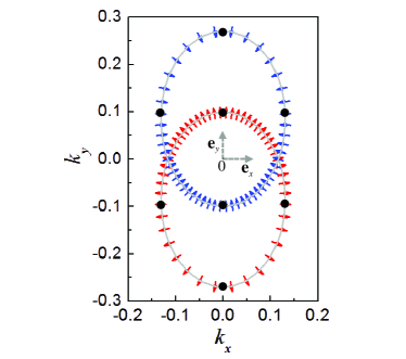
Figure 3: Texture of electron (red) and hole (blue) group velocities on the Fermi surfaces with $\varepsilon_{+,\mathbf{k}}=0.1$ and $\varepsilon_{-,\mathbf{k}}=-0.1$. The Fermi surfaces are shifted ellipses with noncolinear momenta and group velocities, and the group velocities (black dots) on the vertices of semimajor (semiminor) axis are parallel to ${\mathbf{e}}_{y}$ (${\mathbf{e}}_{x}$) of the Cartesian coordinate system $x-y$.

Turning to the group velocity $\mathbf{v}_{\lambda}(\varepsilon,\mathbf{k})=(v_{\lambda,x},v_{\lambda,y})$ of anisotropic tilted MDFs, which has the components

$$v_{\lambda,x} \equiv\frac{\partial\varepsilon_{\lambda,\mathbf{k}}}{\partial k_{x}}=\frac{\lambda v_{x}k_{x}}{\sqrt{k_{x}^{2}+\gamma_{1}^{2}k_{y}^{2}}},$$ (17a)

$$v_{\lambda,y} \equiv\frac{\partial\varepsilon_{\lambda,\mathbf{k}}}{\partial k_{y}}=v_{t}+\frac{\lambda v_{x}\gamma_{1}^{2}k_{y}}{\sqrt{k_{x}^{2}+\gamma_{1}^{2}k_{y}^{2}}}.$$ (17b)

Eq. 17 shows that the electron and hole group velocities are related to each other through $$\mathbf{v}_{+}(\varepsilon,\mathbf{k})=\mathbf{v}_{-}(-\varepsilon,-\mathbf{k}) \varepsilon_{+,\mathbf{k}}=0.1 \varepsilon_{-,\mathbf{k}}=-0.1 {\mathbf{e}}_{y} {\mathbf{e}}_{x} x-y$$. In Fig. 3, we show the texture of electron (red color) and hole (blue color) group velocities on the Fermi surfaces with and . Due to the anisotropy and tilt, the Fermi surface is a shifted ellipse with its semimajor (semiminor) axis parallel to () of the Cartesian coordinate system , and has noncolinear momenta and group velocities Zhang and Yang (2018). The velocity textures for electrons and holes shown by Fig. 3 have the inversion symmetry in the momentum space consistent with Eq. 17.

On the classical trajectory with the momentum $\mathbf{k}_{s}^{c}=(k_{x,s}^{c},k_{y,s}^{c})$, one can obtain

$$\frac{v_{\lambda,y}^{c}}{v_{\lambda,x}^{c}}=\tan\theta.$$ (18)

As a result, $\mathbf{v}_{\lambda}^{c}(\varepsilon,\mathbf{k}_{s}^{c})\mathbf{\parallel R}$ for the classical trajectory, this implies $\mathbf{G}(\mathbf{R},\varepsilon)$ are mainly contributed by the states with the group velocities parallel to the connecting vector $\mathbf{R}$. For convenience, we introduce $\mathbf{v}_{\lambda}^{c}(\varepsilon,\mathbf{R})\equiv\mathbf{v}_{\lambda}^{c}(\varepsilon,\mathbf{k}_{s}^{c})$. $\mathbf{v}_{\lambda}^{c}(\varepsilon,\mathbf{R})\mathbf{\parallel R}$ for the classical trajectory provides one principle to identify the dominant momentum states contributing to real-space GF $\mathbf{G}(\mathbf{R},\varepsilon)$, i.e., through comparing the direction of the group velocity of each state on the Fermi surface and that of $\mathbf{R}$. As an application of this skill, we give an example to consider $\mathbf{G}(\mathbf{R},\varepsilon)$ for electrons without loss of generality. According to the velocity texture shown in Fig. 3, the dominant contributing momentum states on the electron Fermi surface lie on the right (left) vertex of semiminor axis for $\mathbf{G}(\mathbf{R},\varepsilon)$ along the positive (negative) $x$-axis which is consistent with Eq. 15 with $\theta=0$ and $\pi$:

$$k_{x,\pm}^{c} =\pm\frac{\epsilon\gamma_{1}}{\sqrt{\gamma_{1}^{2}-\gamma_{2}^{2}}},$$ (19a)

$$k_{y,\pm}^{c} =-\frac{\epsilon\gamma_{2}}{\gamma_{1}^{2}-\gamma_{2}^{2}}.$$ (19b)

Noting here $$k_{y,\pm}^{c} y \mathbf{G}(\mathbf{R},\varepsilon) y \theta=\pm\pi/2$$ adopt one value and equal to the shifted momentum of the center of the elliptical Fermi surface away from the coordinate originZhang and Yang (2018), which helps to determine the momentum position of semiminor axis in the direction. Similarly, the dominant contributing momentum states on the electron Fermi surface lie on the upper (bottom) vertex of semmajor axis for along the positive (negative) -axis, which is consistent with Eq. 15 with :

$$k_{x,\pm}^{c} =0,$$ (20a)

$$k_{y,\pm}^{c} =\frac{\epsilon}{\gamma_{2}\pm\gamma_{1}}.$$ (20b)

Therefore, it is an effective principle to identify the dominant contributing momentum states to GF by using the velocity texture on the Fermi surface, and this principle should be very useful for the complex Fermi surfaces without analytical solutions.

II.2.3 Analytical GF

Near the classical trajectory, the Taylor expansion of $\phi_{s}(k_{y})$ is

$$\phi_{s}(k_{y},\mathbf{R})=\phi_{s}^{c}(\mathbf{R})-\alpha_{s}(k_{y}-k_{y,s}^{c})^{2}+o(k_{y}),$$ (21)

where $\phi_{s}^{c}(\mathbf{R})\equiv\phi_{s}^{c}(k_{y,s}^{c},\mathbf{R})$ since the $\mathbf{R}$ determines $k_{y,s}^{c}$ for a fixed Fermi surface, $o(k_{y})$ is the high-order small quantity as the function of $k_{y}$ and

$$\alpha_{s}=-\frac{1}{2}\frac{\partial^{2}\phi_{s}}{\partial k_{y}^{2}}|_{k_{y,s}^{c}}=\frac{x\epsilon^{2}\gamma_{1}^{2}}{2(k_{x,s}^{c})^{3}}.$$ (22)

In light of the stationary phase approximation, the real-space GF at the large distance is contributed mainly by the electron propagation along the classical trajectory. As a result, the real-space GF can be expressed analytically as:

$$\mathbf{G}(\mathbf{R},\varepsilon) \approx\frac{\text{sgn(}x\text{)}e^{i\phi_{s}^{c}}}{2\pi}\frac{\epsilon-\gamma_{2}k_{y,s}^{c}}{iv_{x}k_{x,s}^{c}}\sqrt{\frac{\pi}{i\alpha_{s}}}|u_{\lambda}(k_{x,s}^{c},k_{y,s}^{c})\rangle\langle u_{\lambda}(k_{x,s}^{c},k_{y,s}^{c})|,$$ (23a)

$$=\frac{e^{i\phi_{s}^{c}-\lambda\pi/4}}{2\pi}\frac{\epsilon-\gamma_{2}k_{y,s}^{c}}{i\lambda v_{x}|k_{x,s}^{c}|}\sqrt{\frac{\pi}{|\alpha_{s}|}}|u_{\lambda}(k_{x,s}^{c},k_{y,s}^{c})\rangle\langle u_{\lambda}(k_{x,s}^{c},k_{y,s}^{c})|,$$ (23b)

Here, the Gaussian formula $$\int_{-\infty}^{\infty}e^{-\alpha x^{2}}dx=\sqrt{\pi/\alpha} \alpha \arg(\alpha)\in(-\pi,\pi] \sqrt{\alpha}=\sqrt{\left|\alpha\right|}e^{i\arg(\alpha)/2}$$ has been used. And is a complex variable with the angle , so . It is worthy to emphasize that Eq. 23 is consistent with Eq. 11 and has a clear symmetry origin, i.e., the inversion symmetry of velocity textures for electrons and holes as shown by Fig. 3.

III Results and discussions

In order to clearly present the numerical and analytical results for the RKKY interaction in 8-Pmmn borophene, we introduce the scaled RKKY range function ${\mathcal{J}}_{jj^{\prime}}=J_{jj^{\prime}}R^{2}/J_{0}^{2}$ with $R=\left|\mathbf{R}\right|$. Fig. 4(a) and (b) show the RKKY range function ${\mathcal{J}}_{11}$ for the connection vector $\mathbf{R}$ between two impurities along $x$-axis and $y$-axis, in which the red dashed lines are plotted by using the results of exact numerical calculations based on the Eqs. 4 and 10.

III.1 Negligible sublattice and valley effect

In the unit cell of 8-Pmmn borophene, there are 8 boron atoms, among which two are nonequivalent and maybe regarded as the sublattice degree of freedom in analogy to grapheneSherafati and Satpathy (2011); Hsu et al. (2015). Now, the respective contribution of different orbitals of different atoms to form the Dirac states of 8-Pmmn borophene is still in debateZabolotskiy and Lozovik (2016). The low-energy spectrum of 8-Pmmn borophene is expressed in a proper basis, which has no clear connection with the nonequivalent atoms in contrast to the case in graphene. So using the low-energy spectrum of 8-Pmmn borophene, we can just discuss the orbital-dependent RKKY interaction as done in three-dimensional Dirac semimetalsMastrogiuseppe et al. (2016).

The carrier-mediated RKKY interaction is determined by the GF of carriers (cf. Eq. 4). The 8-Pmmn borophene has two inequivalent Dirac cones which can be included in the calculation of GF by combing two valley-dependent GFs. The combination should be a sum of valley-dependent GFs weighed by proper phase factorsBena and Montambaux (2009); Sherafati and Satpathy (2011). The phase factors can be identified through the low-energy expansion of the lattice model. At present, the lattice model for 8-Pmmn borophene is very tediousZabolotskiy and Lozovik (2016), so the phase factors are not known. Even if two valleys can be included properly, their interference only cause the short-range oscillation decorated on the RKKY interaction as a function of impurity distance. Due to the large momentum spacing between two valleysZabolotskiy and Lozovik (2016), the short-range oscillation is on the atomic scale.

Here, we consider the RKKY interaction in the doped 8-Pmmn borophene, and focus its long-range oscillation determined by the Fermi wavelength on the nanometer scale, decay rate determined by the system dimension and the envelop amplitude without dependence on the oscillation detail. Therefore, the sublattice effect and valley effect are negligible in our study.

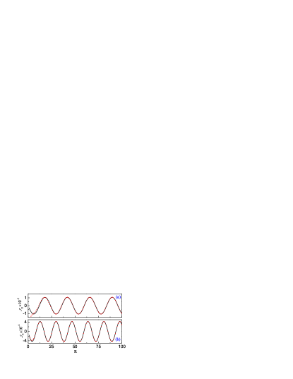
Figure 4: RKKY range function ${\mathcal{J}}_{11}$ for the connection vector between two impurities along $x$-axis (a) and $y$-axis (b). In the plots, we have used the analytical formula (black solid lines) and numerical calculations (red dotted lines) for the electron doping $\varepsilon_{F}=0.1$.

III.2 Analytical expressions for RKKY interaction

To understand the unique behaviors of RKKY interaction mediated by anisotropic and tilted MDFs in 8-Pmmn borophene, we derive the analytical formula for $J_{jj^{\prime}}$. At large distances, the integrand in Eq. 4 can be rewritten as

$$\digamma_{jj^{\prime}}(\varepsilon,\mathbf{R})=\digamma_{jj^{\prime}}^{0}(\varepsilon,\mathbf{R})e^{i\phi_{s}(\mathbf{R})+i\phi_{-s}(-\mathbf{R})}$$ (24)

where $\digamma_{jj^{\prime}}^{0}(\varepsilon,\mathbf{R})$ is a slowly-varying function of the energy. Due to the rapid oscillation of the phase factor $e^{i\phi_{s}(\mathbf{R})+i\phi_{-s}(-\mathbf{R})}$, the integral over energy in Eq. 4 is dominated by the contributions near the Fermi energy $\varepsilon_{F}$, so we can perform the expansion as follows:

$$\phi_{s}(\mathbf{R})+\phi_{-s}(-\mathbf{R})\approx\phi_{s}^{c}(\mathbf{R})+\phi_{-s}^{c}(-\mathbf{R})+\frac{R}{\bar{v}_{\lambda}^{c}(\varepsilon_{F})}(\varepsilon-\varepsilon_{F}),$$ (25)

with

$$\frac{1}{\bar{v}_{\lambda}^{c}(\varepsilon_{F})}=\frac{1}{v_{\lambda}^{c}(\varepsilon_{F},\mathbf{R})}+\frac{1}{v_{\lambda}^{c}(\varepsilon_{F},-\mathbf{R})}.$$ (26)

Here, we have used $\mathbf{v}_{\lambda}^{c}(\varepsilon_{F},\pm\mathbf{R)\parallel(\pm R)}$ on the classical trajectories (cf. classical trajectories in Sec. II.B). We further make the approximation $\digamma_{jj^{\prime}}^{0}(\varepsilon,\mathbf{R})=\digamma_{jj^{\prime}}^{0}(\varepsilon_{F},\mathbf{R})$ for the slowly-varying function, then the RKKY range function becomes

$$J_{jj^{\prime}}(\varepsilon_{F},\mathbf{R})\approx\frac{J_{0}^{2}\bar{v}_{\lambda}(\varepsilon_{F})}{2\pi R}\operatorname{Re}[\digamma_{jj^{\prime}}^{0}(\varepsilon_{F},\mathbf{R})e^{i\phi_{s}^{c}(\mathbf{R})+i\phi_{-s}^{c}(-\mathbf{R})}].$$ (27)

The  analytical formula Eq. 27 implies that the RKKY interaction is determined by the momentum states with group velocities parallel to the connection vector $\mathbf{R}$ between two magnetic impurities and with the energies equal to Fermi level $\varepsilon_{F}$ as shown by the straight solid lines in Fig. 2(b). In contrast, Eq. 4 has an explicit integral over energy and an implicit integral over momentum for GF, so the contributions of all momentum states below $\varepsilon_{F}$ to the RKKY interaction should be considered. Therefore, Eq. 27 provides a simplified version and a physically transparent expression of Eq. 4. Eq. 27 has an immediate application, which leads to

$$\mathbf{J}(\varepsilon_{F},\mathbf{R})=(\mathbf{J}(-\varepsilon_{F},\mathbf{R}))^{\text{T}}.$$ (28)

with the range function matrix

$$\mathbf{J=}\left[\begin{array}[c]{cc}J_{11}&J_{12}\\ J_{21}&J_{22}\end{array}\right]$$ (29)

by recalling Eq. 11 (cf. symmetry discussions in Sec. II.B). This range function relation originates from the inversion symmetry of velocity textures for electrons and holes as shown by Fig. 3, which favors our discussions limited to electron doping case in our study. Eq. 27 is also used to plot the black solid lines in Figs. 4. At large distances, the results of analytical formula and numerical calculations agree very well with each other, so Eq. 27 can capture the main features of long-range RKKY interaction.

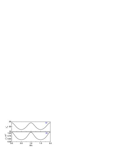
Figure 5: The oscillation period $\lambda_{F}^{+}$ (a) and the envelop amplitude (b) of RKKY range function. Here, $\varepsilon_{F}=0.1$.

III.3 Velocity-determined RKKY interaction and its implications

Firstly, the decay rate of RKKY interaction is $J_{jj^{\prime}}(\varepsilon_{F},\mathbf{R})\propto 1/R^{2}$ since $\digamma_{jj^{\prime}}(\varepsilon_{F},\mathbf{R})$ $\propto 1/R$ by referring to Eqs. 5 and 23, this dimension-determined decay behavior is as that in conventional two-dimensional electron gases Fischer and Klein (1975); Béal-Monod (1987) and in other doped Dirac materials with two-dimensional isotropic MDFs Saremi (2007); Brey et al. (2007); Hwang and Das Sarma (2008); Sherafati and Satpathy (2011); Kogan (2011); Liu et al. (2009); Zhu et al. (2011); Abanin and Pesin (2011).

Secondly, the oscillation period of $J_{jj^{\prime}}(\varepsilon_{F},\mathbf{R})$ is determined by the phase factor $\phi_{s}^{c}(\mathbf{R})+\phi_{-s}^{c}(-\mathbf{R})$, which is given by

$$\lambda_{F}^{s}=\frac{2\pi R}{\left|\phi_{s}^{c}(\mathbf{R})+\phi_{-s}^{c}(-\mathbf{R})\right|}$$ (30)

for the fixing Fermi level $\varepsilon_{F}$. To consider $\varepsilon_{F}=0.1$, we use Eq. 30 to plot the oscillation period in Fig. 5(a) as the function azimuthal $\theta$ of the connection vector $\mathbf{R}$. Fig. 5(a) has the mirror symmetry about $y$-axis originating from the symmetry of Hamiltonian Sadhukhan and Agarwal (2017), and shows two peaks (valleys) along $\pm x$-axis ($\pm y$-axis). We defines the peak-valley ratio as the anisotropy degree of the oscillation period. Referring to Eq. 15, for $\varepsilon_{F}>0$, one can obtain $\lambda_{F}^{+}(\theta=0)=\pi({\gamma_{1}^{2}-\gamma_{2}^{2}})^{1/2}/(\epsilon_{F}\gamma_{1})$ and $\lambda_{F}^{+}(\theta=\frac{\pi}{2})=\pi(\gamma_{1}^{2}-\gamma_{2}^{2})/(\epsilon_{F}\gamma_{1})$, which both show the inverse linear energy dependence of the oscillation period identical to the case for the isotropic MDFs Sherafati and Satpathy (2011); Zhu et al. (2011). In particular, in Fig. 5(a), $\lambda_{F}^{+}(\theta=0)=24$ and $\ \lambda_{F}^{+}(\theta=\pi/2)=17$ when $\varepsilon_{F}=0.1$ for the RKKY range function along $x$-axis and $y$-axis, respectively. As a result, the anisotropy degree of the oscillation period is a constant $v_{x}/({v_{y}^{2}-v_{t}^{2}})^{1/2}\approx 1.4$ independent of the Fermi energy $\varepsilon_{F}$.

Thirdly, the envelope amplitude of the oscillating RKKY interaction is another important feature beyond the decay rate and oscillation period. The envelope amplitude depends linearly on Fermi level $\varepsilon_{F}$ by combing Eqs. 23 and 27 and by using $\alpha_{s}\propto\varepsilon^{2}$ in Eq. 22. In Fig. 5(b), Eqs. 23 and 27 are used to plot the envelope amplitude of RKKY interaction $J_{11}$ as the function azimuthal $\theta$ of $\mathbf{R}$. In analogy to the oscillation period, we also define peak-valley ratio as the anisotropy degree for the envelope amplitude, which can be extracted analytically from Eqs. 23 and 27 and is a constant $v_{x}^{2}v_{y}^{2}/(v_{y}^{2}-v_{t}^{2})^{2}\approx 2.5$ independent of the Fermi energy $\varepsilon_{F}$.

As a result, the RKKY mediated by the anisotropic and tilted MDFs has anisotropic features in its oscillation period and envelop amplitude but does not change its decay rate. The spatial anisotropy is an usual feature of RKKY interaction, at least on the atomic scale considering the discrete lattice nature of host materials, and the spatially anisotropic RKKY interaction has been reported in experiementZhou et al. (2010); Sessi et al. (2016a). Theoretically, there are quite a few studies on the close relation between anisotropic RKKY interaction in long range (on the scale of Fermi wavelength) and band features of various materials, e.g., III-V diluted magnetic semiconductorsTimm and MacDonald (2005), semiconductor quantum wiresZhu et al. (2010), surface states on Pt(111)Patrone and Einstein (2012), the surface of the topological insulator Bi₂Se₃Li et al. (2012), spin-polarized grapheneParhizgar et al. (2013b), three-dimensional Dirac semimetalsMastrogiuseppe et al. (2016), three-dimensional electron gases with linear spin-orbit couplingWang et al. (2017), and phosphorene withDuan et al. (2017) and without mechanical strainZare et al. (2018), and so on. However, comparing to the other materials, the anisotropic RKKY interaction in 8-Pmmn borophene is independent of the Fermi energy $\varepsilon_{F}$ but is velocity-determined, which has two significant implications. On one hand, the velocity-determined RKKY interaction fully determines the band dispersion described by three velocities $v_{x,y,t}$ (cf. band dispersion of Eq. 2), this provides an alternative way to characterize the band dispersion. And the RKKY interaction has also proposed to probe the topological phase transition in silicene nanoribbonZare et al. (2016) and quasiflat edge modes in phosphorene nanoribbonZare and Sadeghi (2018); Islam et al. (2018). On the other hand, the anisotropy of RKKY interaction is expected to be tunable by choosing other Dirac materials with different $v_{x,y,t}$ (e.g., quinoid-type graphene and $\alpha$-(BEDT-TTF)₂I₃Goerbig et al. (2008)) and even by tuning $v_{x,y,t}$ in the same Dirac material (e.g., graphene under strainNaumis et al. (2017)). In Dirac materials, the RKKY interaction leads to the ordering of magnetic impurities as discussed theoreticallyLiu et al. (2009); Efimkin and Galitski (2014); Min et al. (2017); Park et al. (2018) and demonstrated experimentallySessi et al. (2014, 2016b); Wang et al. (2018). Based on the velocity-determined RKKY interaction mediated by anisotropic tilted MDFs, new anisotropy-induced magnetic properties are expected and has high tunability. Therefore, we hope this study is helpful to the physical understanding of 8-Pmmn borophene and its possible applications in spin fields.

IV Conclusions

In this study, we investigate the RKKY interaction mediated by the anisotropic and tilted MDFs in 8-Pmmn borophene. In the long range, the RKKY interaction is mainly contributed by the limited momentum states with group velocities parallel to the connection vector $\mathbf{R}$ between two magnetic impurities and with the energies equal to Fermi level $\varepsilon_{F}$. As a result, we analytically demonstrate that the RKKY interaction in 8-Pmmn borophene has the usual decay rate as in the other two-dimensional materials, but is anisotropic in its oscillation period and envelop amplitude with the explicit velocity dependence $v_{x}/({v_{y}^{2}-v_{t}^{2}})^{1/2}$ and $v_{x}^{2}v_{y}^{2}/(v_{y}^{2}-v_{t}^{2})^{2}$. The velocity-determined RKKY interaction implies its usefulness to fully characterize the band dispersion of 8-Pmmn borophene and other similar Dirac materials, and its tunability by engineering the anisotropic tilted MDFs. In addition, the velocity-determined RKKY interaction should be observable in present experiment since the evidence of RKKY interaction mediated by anisotropic MDFs on surface Mn-doped Bi₂Te₃ has been reported through focusing interference patterns observed by scanning tunneling microscopySessi et al. (2016a). This study is relevant to spatial propagation properties of novel anisotropic tilted MDFs, and shows the potential spin application of 8-Pmmn borophene.

Note added. Recently, we became aware of a related preprintPaul et al. (2018), which studies the RKKY interaction in 8-Pmmn borophene along two specific directions.

References

- Žutić et al. (2004) I. Žutić, J. Fabian, and S. Das Sarma, Rev. Mod. Phys. 76, 323 (2004).
- Fert (2008) A. Fert, Rev. Mod. Phys. 80, 1517 (2008).
- Power and Ferreira (2013) S. R. Power and M. S. Ferreira, Crystals 3, 49 (2013).
- Ruderman and Kittel (1954) M. A. Ruderman and C. Kittel, Phys. Rev. 96, 99 (1954).
- Kasuya (1956) T. Kasuya, Prog. Theor. Phys. 16, 45 (1956).
- Yosida (1957) K. Yosida, Phys. Rev. 106, 893 (1957).
- Jungwirth et al. (2006) T. Jungwirth, J. Sinova, J. Mašek, J. Kučera, and A. H. MacDonald, Rev. Mod. Phys. 78, 809 (2006).
- Wolf et al. (2001) S. A. Wolf, D. D. Awschalom, R. A. Buhrman, J. M. Daughton, S. von Molnar, M. L. Roukes, A. Y. Chtchelkanova, and D. M. Treger, Science 294, 1488 (2001).
- MacDonald et al. (2005) A. H. MacDonald, P. Schiffer, and N. Samarth, Nat. Mater. 4, 195 (2005).
- Loss and DiVincenzo (1998) D. Loss and D. P. DiVincenzo, Phys. Rev. A 57, 120 (1998).
- Trifunovic et al. (2012) L. Trifunovic, O. Dial, M. Trif, J. R. Wootton, R. Abebe, A. Yacoby, and D. Loss, Phys. Rev. X 2, 011006 (2012).
- Piermarocchi et al. (2002) C. Piermarocchi, P. Chen, L. J. Sham, and D. G. Steel, Phys. Rev. Lett. 89, 167402 (2002).
- Craig et al. (2004) N. J. Craig, J. M. Taylor, E. A. Lester, C. M. Marcus, M. P. Hanson, and A. C. Gossard, Science 304, 565 (2004).
- Rikitake and Imamura (2005) Y. Rikitake and H. Imamura, Phys. Rev. B 72, 033308 (2005).
- Friesen et al. (2007) M. Friesen, A. Biswas, X. Hu, and D. Lidar, Phys. Rev. Lett. 98, 230503 (2007).
- Srinivasa et al. (2015) V. Srinivasa, H. Xu, and J. M. Taylor, Phys. Rev. Lett. 114, 226803 (2015).
- Saremi (2007) S. Saremi, Phys. Rev. B 76, 184430 (2007).
- Brey et al. (2007) L. Brey, H. A. Fertig, and S. Das Sarma, Phys. Rev. Lett. 99, 116802 (2007).
- Hwang and Das Sarma (2008) E. H. Hwang and S. Das Sarma, Phys. Rev. Lett. 101, 156802 (2008).
- Sherafati and Satpathy (2011) M. Sherafati and S. Satpathy, Phys. Rev. B 84, 125416 (2011).
- Kogan (2011) E. Kogan, Phys. Rev. B 84, 115119 (2011).
- Parhizgar et al. (2013a) F. Parhizgar, H. Rostami, and R. Asgari, Phys. Rev. B 87, 125401 (2013a).
- Hatami et al. (2014) H. Hatami, T. Kernreiter, and U. Zülicke, Phys. Rev. B 90, 045412 (2014).
- Mastrogiuseppe et al. (2014) D. Mastrogiuseppe, N. Sandler, and S. E. Ulloa, Phys. Rev. B 90, 161403 (2014).
- Ávalos-Ovando et al. (2016a) O. Ávalos-Ovando, D. Mastrogiuseppe, and S. E. Ulloa, Phys. Rev. B 93, 161404 (2016a).
- Ávalos-Ovando et al. (2016b) O. Ávalos-Ovando, D. Mastrogiuseppe, and S. E. Ulloa, Phys. Rev. B 94, 245429 (2016b).
- Ávalos-Ovando et al. (2019) O. Ávalos-Ovando, D. Mastrogiuseppe, and S. E. Ulloa, Phys. Rev. B 99, 035107 (2019).
- Liu et al. (2009) Q. Liu, C.-X. Liu, C. Xu, X.-L. Qi, and S.-C. Zhang, Phys. Rev. Lett. 102, 156603 (2009).
- Zhu et al. (2011) J.-J. Zhu, D.-X. Yao, S.-C. Zhang, and K. Chang, Phys. Rev. Lett. 106, 097201 (2011).
- Abanin and Pesin (2011) D. A. Abanin and D. A. Pesin, Phys. Rev. Lett. 106, 136802 (2011).
- Hsu et al. (2017) C.-H. Hsu, P. Stano, J. Klinovaja, and D. Loss, Phys. Rev. B 96, 081405 (2017).
- Hsu et al. (2018) C.-H. Hsu, P. Stano, J. Klinovaja, and D. Loss, Phys. Rev. B 97, 125432 (2018).
- Zhang et al. (2018) S.-H. Zhang, J.-J. Zhu, W. Yang, and K. Chang, arXiv:1812.02281 (2018).
- Zare et al. (2016) M. Zare, F. Parhizgar, and R. Asgari, Phys. Rev. B 94, 045443 (2016).
- Duan et al. (2018) H.-J. Duan, C. Wang, S.-H. Zheng, R.-Q. Wang, D.-R. Pan, and M. Yang, Scientific Reports 8, 6185 (2018).
- Duan et al. (2017) H. Duan, S. Li, S.-H. Zheng, Z. Sun, M. Yang, and R.-Q. Wang, New Journal of Physics 19, 103010 (2017).
- Zare and Sadeghi (2018) M. Zare and E. Sadeghi, Phys. Rev. B 98, 205401 (2018).
- Islam et al. (2018) S. F. Islam, P. Dutta, A. M. Jayannavar, and A. Saha, Phys. Rev. B 97, 235424 (2018).
- Masrour et al. (2016) R. Masrour, A. Jabar, A. Benyoussef, and M. Hamedoun, Journal of Magnetism and Magnetic Materials 401, 695 (2016).
- Jabar and Masrour (2017) A. Jabar and R. Masrour, Solid State Communications 268, 38 (2017).
- Jabar and Masrour (2018) A. Jabar and R. Masrour, Chemical Physics Letters 700, 130 (2018).
- Jabar et al. (2019) A. Jabar, R. Masrour, A. Benyoussef, and M. Hamedoun, Physica A: Statistical Mechanics and its Applications 523, 915 (2019).
- Hosseini and Askari (2015) M. V. Hosseini and M. Askari, Phys. Rev. B 92, 224435 (2015).
- Chang et al. (2015) H.-R. Chang, J. Zhou, S.-X. Wang, W.-Y. Shan, and D. Xiao, Phys. Rev. B 92, 241103(R) (2015).
- Mastrogiuseppe et al. (2016) D. Mastrogiuseppe, N. Sandler, and S. E. Ulloa, Phys. Rev. B 93, 094433 (2016).
- Zhou et al. (2014) X.-F. Zhou, X. Dong, A. R. Oganov, Q. Zhu, Y. Tian, and H.-T. Wang, Phys. Rev. Lett. 112, 085502 (2014).
- Lopez-Bezanilla and Littlewood (2016) A. Lopez-Bezanilla and P. B. Littlewood, Phys. Rev. B 93, 241405 (2016).
- Zabolotskiy and Lozovik (2016) A. D. Zabolotskiy and Y. E. Lozovik, Phys. Rev. B 94, 165403 (2016).
- Nakhaee et al. (2018a) M. Nakhaee, S. A. Ketabi, and F. M. Peeters, Phys. Rev. B 97, 125424 (2018a).
- Nakhaee et al. (2018b) M. Nakhaee, S. A. Ketabi, and F. M. Peeters, Phys. Rev. B 98, 115413 (2018b).
- Sadhukhan and Agarwal (2017) K. Sadhukhan and A. Agarwal, Phys. Rev. B 96, 035410 (2017).
- Verma et al. (2017) S. Verma, A. Mawrie, and T. K. Ghosh, Phys. Rev. B 96, 155418 (2017).
- Islam and Jayannavar (2017) S. F. Islam and A. M. Jayannavar, Phys. Rev. B 96, 235405 (2017).
- Champo and Naumis (2019) A. E. Champo and G. G. Naumis, Phys. Rev. B 99, 035415 (2019).
- Mannix et al. (2015) A. J. Mannix, X.-F. Zhou, B. Kiraly, J. D. Wood, D. Alducin, B. D. Myers, X. Liu, B. L. Fisher, U. Santiago, J. R. Guest, et al., Science 350, 1513 (2015).
- Feng et al. (2016) B. Feng, J. Zhang, Q. Zhong, W. Li, S. Li, H. Li, P. Cheng, S. Meng, L. Chen, and K. Wu, Nature Chemistry 8, 563 (2016).
- Feng et al. (2017) B. Feng, O. Sugino, R.-Y. Liu, J. Zhang, R. Yukawa, M. Kawamura, T. Iimori, H. Kim, Y. Hasegawa, H. Li, et al., Phys. Rev. Lett. 118, 096401 (2017).
- Shi and Jiang (2018) K.-L. Shi and W. Jiang, Physica E: Low-dimensional Systems and Nanostructures 101, 94 (2018).
- Shi et al. (2018) K. Shi, W. Jiang, A. Guo, K. Wang, and C. Wu, Physica A: Statistical Mechanics and its Applications 500, 11 (2018).
- Zou et al. (2018) C.-L. Zou, D.-Q. Guo, F. Zhang, J. Meng, H.-L. Miao, and W. Jiang, Physica E: Low-dimensional Systems and Nanostructures 104, 138 (2018).
- Klinovaja and Loss (2013) J. Klinovaja and D. Loss, Phys. Rev. B 87, 045422 (2013).
- Zhang et al. (2017) S.-H. Zhang, J.-J. Zhu, W. Yang, and K. Chang, 2D Materials 4, 035005 (2017).
- Roth et al. (1966) L. M. Roth, H. J. Zeiger, and T. A. Kaplan, Phys. Rev. 149, 519 (1966).
- Liu et al. (2012) Q. Liu, X.-L. Qi, and S.-C. Zhang, Phys. Rev. B 85, 125314 (2012).
- Power and Ferreira (2011) S. R. Power and M. S. Ferreira, Phys. Rev. B 83, 155432 (2011).
- Lounis et al. (2011) S. Lounis, P. Zahn, A. Weismann, M. Wenderoth, R. G. Ulbrich, I. Mertig, P. H. Dederichs, and S. Blügel, Phys. Rev. B 83, 035427 (2011).
- Zhang and Yang (2018) S.-H. Zhang and W. Yang, Phys. Rev. B 97, 235440 (2018).
- Hsu et al. (2015) C.-H. Hsu, P. Stano, J. Klinovaja, and D. Loss, Phys. Rev. B 92, 235435 (2015).
- Bena and Montambaux (2009) C. Bena and G. Montambaux, New Journal of Physics 11, 095003 (2009).
- Fischer and Klein (1975) B. Fischer and M. W. Klein, Phys. Rev. B 11, 2025 (1975).
- Béal-Monod (1987) M. T. Béal-Monod, Phys. Rev. B 36, 8835 (1987).
- Zhou et al. (2010) L. Zhou, J. Wiebe, S. Lounis, E. Vedmedenko, F. Meier, S. Blugel, P. H. Dederichs, and R. Wiesendanger, Nat. Phys. 6, 187 (2010).
- Sessi et al. (2016a) P. Sessi, P. Rüßmann, T. Bathon, A. Barla, K. A. Kokh, O. E. Tereshchenko, K. Fauth, S. K. Mahatha, M. A. Valbuena, S. Godey, et al., Phys. Rev. B 94, 075137 (2016a).
- Timm and MacDonald (2005) C. Timm and A. H. MacDonald, Phys. Rev. B 71, 155206 (2005).
- Zhu et al. (2010) J.-J. Zhu, K. Chang, R.-B. Liu, and H.-Q. Lin, Phys. Rev. B 81, 113302 (2010).
- Patrone and Einstein (2012) P. N. Patrone and T. L. Einstein, Phys. Rev. B 85, 045429 (2012).
- Li et al. (2012) Z. L. Li, J. H. Yang, G. H. Chen, M.-H. Whangbo, H. J. Xiang, and X. G. Gong, Phys. Rev. B 85, 054426 (2012).
- Parhizgar et al. (2013b) F. Parhizgar, R. Asgari, S. H. Abedinpour, and M. Zareyan, Phys. Rev. B 87, 125402 (2013b).
- Wang et al. (2017) S.-X. Wang, H.-R. Chang, and J. Zhou, Phys. Rev. B 96, 115204 (2017).
- Zare et al. (2018) M. Zare, F. Parhizgar, and R. Asgari, Journal of Magnetism and Magnetic Materials 456, 307 (2018).
- Goerbig et al. (2008) M. O. Goerbig, J.-N. Fuchs, G. Montambaux, and F. Piéchon, Phys. Rev. B 78, 045415 (2008).
- Naumis et al. (2017) G. G. Naumis, S. Barraza-Lopez, M. Oliva-Leyva, and H. Terrones, Reports on Progress in Physics 80, 096501 (2017).
- Efimkin and Galitski (2014) D. K. Efimkin and V. Galitski, Phys. Rev. B 89, 115431 (2014).
- Min et al. (2017) H. Min, E. H. Hwang, and S. Das Sarma, Phys. Rev. B 95, 155414 (2017).
- Park et al. (2018) S. Park, H. Min, E. H. Hwang, and S. Das Sarma, Phys. Rev. B 98, 064425 (2018).
- Sessi et al. (2014) P. Sessi, F. Reis, T. Bathon, K. A. Kokh, O. E. Tereshchenko, and M. Bode, Nature Communications 5, 5349 (2014).
- Sessi et al. (2016b) P. Sessi, R. R. Biswas, T. Bathon, O. Storz, S. Wilfert, A. Barla, K. A. Kokh, O. E. Tereshchenko, K. Fauth, M. Bode, et al., Nature Communications 7, 12027 (2016b).
- Wang et al. (2018) W. Wang, Y. Ou, C. Liu, Y. Wang, K. He, Q.-K. Xue, and W. Wu, Nature Physics 14, 791 (2018).
- Paul et al. (2018) G. C. Paul, S. Firoz Islam, and A. Saha, arXiv:1811.08301 (2018).