Fast Hyperparameter Tuning using Bayesian Optimization with Directional Derivatives

Abstract

In this paper, we develop a Bayesian optimization based hyperparameter tuning framework inspired by statistical learning theory for classifiers. We utilize two key facts from PAC learning theory; the generalization bound will be higher for a small subset of data compared to the whole, and the highest accuracy for a small subset of data can be achieved with a simple model. We initially tune the hyperparameters on a small subset of training data using Bayesian optimization. While tuning the hyperparameters on the whole training data, we leverage the insights from the learning theory to seek more complex models. We realize this by using directional derivative signs strategically placed in the hyperparameter search space to seek a more complex model than the one obtained with small data. We demonstrate the performance of our method on the tasks of tuning the hyperparameters of several machine learning algorithms.

Introduction

Hyperparameter tuning is a challenging problem in machine learning. Bayesian optimization has emerged as an efficient framework for hyperparameter tuning, outperforming most conventional methods such as grid search and random search (?; ?). It offers robust solutions for optimizing expensive black-box functions, using a non-parametric Gaussian Process (?) as a probabilistic measure to model the unknown function. A surrogate utility function, known as acquisition function guides the search for the next observation. The acquisition function continually trades-off two key aspects: exploring regions where epistemic uncertainty about the function is high and exploiting regions where the predictive mean is high. The use of Bayesian optimization for efficient hyperparameter tuning of complex models have been first proposed in (?). Despite the advances, hyperparameter tuning on large datasets remains challenging.

Early attempt to make Bayesian optimization efficient includes multi-task Bayesian optimization (?) to optimize hyperparameters of the whole data in presence of an auxiliary problem of hyperparameter optimization for a small subset of data. They proceed by estimating task relationship, then finding best parameters for these tasks simultaneously within the same framework. First, it is inefficient because both the cheap and expensive processes are being discovered simultaneously, making early estimate of their relationship poor, and thus delaying convergence. Second, it is not straightforward to design a task-to-task covariance function to leverage on how the hyperparameters are related across these two tasks.

An alternate approach has been attempted in (?) where they assume that performance of a hyperparameter on a smaller subset of data can be used to predict the performance of the same hyperparameter on the whole data. This frees them from directly evaluating on the larger dataset. Their assumption, however, is poorly grounded on learning theory. The authors of (?) developed a similar strategy where a multi-fidelity optimization technique has been used to approximate the expensive functions. Their work also have not leveraged any task-specific knowledge from learning theory. Recently, authors of (?) have developed a multi-arm bandit based strategy, called Hyperband algorithm. Hyperband uses a strategy that allocates a finite resource (data samples, iteration) budget to randomly sampled configurations, and choose the configurations that are expected to perform well based on their performance on the subset of data. Hyperband makes sure that only promising hyperparameters proceed to the next round, and less promising configurations are discarded. Their hypothesis, however, does not hold for hyperparameters that directly control the model complexity, e.g. cost parameter C in support vector machines (SVM). One instance of such a hyperparameter may work well on a subset of data but the same may perform poorly on the larger data. Time as resource may be useful when a gradient descent type of algorithm can be used, but not for other kinds of optimization routines as many do not guarantee smooth convergence. This restricts the application of Hyperband to tuning hyperparameters that are functions of data topology (learning rate, momentum, etc.), and when the model is trained using gradient descent based algorithms.

We seek our inspiration from PAC learning theory (?) and investigate an alternative approach for hyperparameter tuning by utilizing key concepts about model complexity and generalization performance with respect to dataset size:

• Vapnik–Chervonenkis inequality - The bound on the difference between empirical error and the generalization error is higher for smaller datasets.

• Vapnik–Chervonenkis dimension - For a small dataset, the smallest generalization error can be achieved with a lower complexity classifier.

  

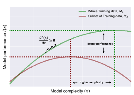
  Figure 1: Schematic representation of generalization performance vs model complexity. We indicate the best performance of the two models and the corresponding model complexities.

We illustrate our intuition in a schematic diagram of generalization performance vs model complexity (Figure 1). Two models are built - one that uses the whole training data ($M_{1}$) and the other only a subset of data ($M_{2}$). The idea is to transfer some knowledge from $M_{2}$ to $M_{1}$. As expected, $M_{1}$ seeks more complex models achieving higher performance - this performance increases monotonically till it saturates. $M_{2}$ on the other hand settles on a lower complex configuration and its generalization performance degrades as it selects more complex models. $M_{2}$ exhibits poorer generalization performance compared to $M_{1}$. Between the lower and upper bounds of the performance in $M_{2}$, the performance of $M_{1}$ rises strictly monotonically. We can use this extra knowledge to tune the hyperparameters of $M_{1}$. We do this by introducing signs of the derivatives (?) (instead of the actual derivative as these are unavailable) as additional observations to the GP modeling $M_{1}$, and show that this results in a faster hyperparameter tuning algorithm. Using this intuition we construct a method termed HyperTune.

We demonstrate the empirical performance of our method on the task of tuning hyperparameters of several machine learning algorithms on real-world datasets. We compare our results against the baselines of Fabolas (?) and Hyeprband (?) and show that our algorithm performs better in almost all the tasks.

Key insights from PAC Generalization Bound by Vapnik and Chervonenkis

We note the main insights in (?) which relates the generalization performance and complexity of the classification models. VC dimension (?) of a hypothesis class $\mathcal{H}\subseteq{0,1}^{\mathcal{X}}$ is defined as:

$$V_{\mathcal{H}}:=\max\left\{n\mid S_{\mathcal{H}}(n)=2^{n}\right\}$$

where $S_{\mathcal{H}}(n)$ is the shatter coefficient (?) and $n$ denotes the number of data points, and is defined as,

$$S_{\mathcal{H}}(n)=:\max_{\mathbf{x}_{1},...,\mathbf{x}_{n}\in\mathcal{X}}N_{\mathcal{H}}(\mathbf{x}_{1},...,\mathbf{x}_{n})$$

where $\mathbf{x}_{1},...,\mathbf{x}_{n}$ denote data points, and $N_{\mathcal{H}}(\mathbf{x}_{1},...,\mathbf{x}_{n}):=|\{(h(\mathbf{x}_{1}),...,h(\mathbf{x}_{n})):h\in\mathcal{H}\}|$. We can relate VC dimension and shatter coefficient using a generalization bound. We recall the theorem and corollary in (?) as:

Theorem 1.

(?) For binary classification and the 0/1 loss function, we have the following generalization bounds,

$$\Pr\left(sup_{h\in\mathcal{H}}\mid\hat{R_{n}}(h)-R(h)\mid>\varepsilon\right)\leq 8S_{\mathcal{H}}\left(n\right)e^{\frac{-ne^{2}}{32}}$$

where the probability is with respect to the draw of the training data. Here $\hat{R_{n}}(h)$ denotes the empirical risk and $R(h)$ denotes the expected generalization risk for a hypothesis $h$.

Corollary 1.

(?) If $\hat{R_{n}}(h)$ is an empirical risk over $\mathcal{H}$, then with probability greater than $1-\delta$, the generalization bound is given as,

$$\hat{R_{n}}(h)\leq R(h)+\sqrt{\dfrac{128\left[V_{\mathcal{H}}\log(n+1)\right]+\log(\frac{8}{\delta})}{n}}$$

From the above Theorem and Corollary, we can conclude that if $n$ is small, then $V_{\mathcal{H}}$ should also be small. For a fixed VC dimension $V_{\mathcal{H}}$, the generalization bound is higher when $n$ is small. It also implies that the lowest generalization risk (highest accuracy) for a model that is trained on a larger data will occur at a more complex model than the one with a smaller training set.

Bayesian Optimization

Bayesian optimization is an elegant framework for sequential optimization of unknown objective functions and can be summarized as, $\mathbf{x}^{*}=\arg\max_{\mathbf{x\in\mathcal{X}}}f(\mathbf{x})$, where $\mathcal{X}\subseteq\mathbb{R}^{D}$. The function evaluations can be noisy with $y=f(\mathbf{x})+\epsilon$ where $\epsilon\sim\mathcal{N}(0,\sigma^{2})$. Gaussian process (GP) (?) is a popular choice for specifying prior over smoothly varying functions. Let $\mathbf{x}$ be a $D$ dimensional observation and $\mathbf{X}$ be a matrix with $p$ such observations. Let $\mathbf{y}$ be the corresponding function values. Without any loss of generality, the prior mean function can be assumed to be a zero function making the Gaussian process fully defined by the covariance function as: $p\left(\text{$\mathbf{f}$}\mid\mathbf{X}\right)=\mathcal{N}(\mathbf{f}\mid 0,\mathbf{K})$ where $\mathbf{f}$ is the corresponding latent variables and $\mathbf{K}$ is the kernel matrix with $\mathbf{K_{\text{i,j}}=k(x_{\text{i}},x_{\text{j}})}$. We choose the popular squared exponential kernel as our choice of the covariance function. It is defined as, $k(\mathbf{\mathbf{x},\mathbf{x^{\prime}}})=exp(-\frac{1}{2\theta}||\mathbf{x}-\mathbf{x^{\prime}}||^{2})$ where $\theta$ is the length-scale parameter of the kernel. Using the properties of Gaussian Process, partial derivatives of a GP is still Gaussian since differentiation is a linear process (?; ?). This allows us to include the derivative of the unknown objective function using the following criteria for covariance functions as:

$$k\left[\frac{\partial f^{(i)}}{\partial x_{d}^{(i)}},f^{(j)}\right]=\frac{\partial}{\partial x_{d}^{(i)}}k\left[f^{(i)},f^{(j)}\right]$$ (1)

$$k\left[\frac{\partial f^{(i)}}{\partial x_{d}^{(i)}},\frac{\partial f^{(j)}}{\partial x_{g}^{(j)}}\right]=\frac{\partial^{2}}{\partial x_{d}^{(i)}\partial x_{g}^{(j)}}k\left[f^{(i)},f^{(j)}\right]$$ (2)

where $d,g\in[1,...,D]$. Bayesian optimization now uses an acquisition function that guides the search for the optimum of the underlying objective function. In this paper, we use the expected improvement (EI) (?) acquisition for its usefulness and simplicity. However, it has to be noted that our method can work with any acquisition function. EI is defined as: $\alpha(\mathbf{x}_{p+1})=(\mu(\mathbf{x}_{p+1})-f(\mathbf{x}^{+}))\Phi(z)+\sigma(\mathbf{x}_{p+1})\phi(z)$ where $z=(\mu(\mathbf{x}_{p+1})-f(\mathbf{x}^{+}))/\sigma(\mathbf{x}_{p+1})$, $\Phi(.)$ and $\phi(.)$ are the CDF and PDF of a standard normal distribution.

HyperTune - A Learning Theory based Hyperparameter Tuning Framework

Consider a hyperparameter tuning task wherein our objective is to maximize validation set accuracy as,

$$\mathbf{x^{*}}=\arg\max_{\mathbf{x\in\mathcal{X}}}f(\mathbf{x})$$

where $\mathcal{X}\subseteq\mathbb{R}^{D}$ and $f(\mathbf{x})$ is performance of the model on validation dataset for a set of hyperparameters $\mathbf{x}$. Let the search bound for different hyperparameters be $[\mathbf{l},\mathbf{u}]$ - $\mathbf{l}$ and $\mathbf{u}$ are $D$ dimensional vectors that denote the lower and the upper bounds, respectively.

While our objective is to optimize hyperparameters on the whole training data, we start by identifying the optimal hyperparameters on a small subset of the training data using Bayesian optimization. These optimal hyperparameters can be noisy as they are built on a small portion of data. We thus pick a robust estimate of the hyperparameter by repeating Bayesian optimization on a number of different smaller subsets and then average the optimal hyperparameters. The performance of the model trained on small data (randomly created) may exhibit spurious pikes that peak either at extremely high complex region or at a very low complex region. In the former case, we may miss the optimal for the larger data whilst the latter turns our algorithm unnecessarily inefficient. Through averaging, we smooth out the spurious behaviours and identify the right complexity for the small data, which is then used to provide directional derivative to effectively have a tighter bound for the larger data. We denote this best hyperparameter from the smaller subset as $\bar{\mathbf{x}}_{s}^{*}$.

Algorithm 1 Sampling Directional Derivative Observations.

1:Bounds on Search space : $[\mathbf{l},\mathbf{u}]$

2:Number of virtual observations : $N$

3:for $b=1,2,..B$ do

4:     $\mathbf{x}_{s,b}^{*}$=$\arg\max_{\mathbf{x\in\mathcal{X}}}f_{s,b}(\mathbf{x})$ $\triangleright$ Conduct Bayesian optimization on small subsets of data

5:end for

6:$\bar{\mathbf{x}}_{s}^{*}=\frac{1}{B}\sum_{b=1}^{B}\mathbf{x}_{s,b}^{*}$

7:$\mathbf{X}_{m}\sim\mathcal{U}(L,\bar{\mathbf{x}}_{s}^{*},N)$

8:for $d=1,2,..D$ do

9:     if $\dfrac{\partial f(\mathbf{x})}{\partial x_{d}}\geq 0$ then

10:         $m_{d}=1$

11:     else if $\dfrac{\partial f(\mathbf{x})}{\partial x_{d}}\leq 0$ then

12:         $m_{d}=-1$

13:     else

14:         $m_{d}=null$

15:     end if

16:end for

While tuning hyperparameters on the whole dataset, we note that for certain hyperparameters which directly controls the model complexity, the generalization performance would be monotonically changing in the bound $[\mathbf{l},\bar{\mathbf{x}}_{s}^{*}]$. If a particular hyperparameter increases the complexity, then the model performance also increases for a larger dataset wherein it decreases otherwise. For example, the model complexity of SVM increases as the cost parameter $C$ increases. The model complexity of elastic net (?) decreases with an increase in the hyperparameter $\alpha$ that determines the magnitude of the penalty term. We exploit such trends by sampling $N$ directional derivative observations $\mathbf{X}_{m}$ uniformly within the range $[\mathbf{l},\bar{\mathbf{x}}_{s}^{*}]$. Using the expert knowledge, we assign a sign that encodes our belief about how the trend will be changing for a model that uses the whole data. Let $\mathbf{m}$ be a vector of directional derivative signs that takes only $1$ or $-1$ indicating whether the function is either monotonically increasing or decreasing. we assign $m_{d}=1$ when $\dfrac{\partial f(\mathbf{x})}{\partial x_{d}}\geq 0$ and $m_{d}=-1$ when $\dfrac{\partial f(\mathbf{x})}{\partial x_{d}}\leq 0$. We consider a hyperparameter as neutral if it does not contribute towards model complexity, in which case we do not encode any directional sign (e.g. learning rate for neural networks). We further detail the procedure for sampling the directional derivatives in Algorithm 1.

Algorithm 2 HyperTune.

1:Input: Initial observations $\{\mathbf{X},\mathbf{y}\}$

2:Directional Derivative Observations $\{\mathbf{X}_{m},{\mathbf{m}}\}$ $\triangleright$ Using Algorithm 1

3:Combined observations $O\equiv\{\mathbf{X},\mathbf{X}_{m},\mathbf{y},\mathbf{m}\}$

4:for $t=1,2,..T$ do

5:     $\mathbf{x}_{t}=\arg\max_{\mathbf{x\in\mathcal{X}}}\alpha(\mathbf{x}|O)$

6:     Evaluate $f(.)$ at $\mathbf{x}_{t}$

7:     $O\equiv{O\cup(\mathbf{x}_{t},\mathbf{y}_{t})}$

8:end for

9:Output: $\{\mathbf{x}_{t},\mathbf{y}_{t}\}_{t=1}^{T}$

Let $\mathbf{X}$ be an initial set of hyperparameters and $\mathbf{y}$ be the corresponding model performances on the whole data. Let $\mathbf{f}$ be the latent function values and $\mathbf{f}^{{}^{\prime}}$ be the corresponding derivative values. The joint prior for latent values and derivatives is also Gaussian as,

$$p\left(\mathbf{f},\mathbf{f}^{\prime}\mid\mathbf{X},\mathbf{X}_{m}\right)=\mathcal{N}(\mathbf{f}_{joint}\mid 0,\mathbf{K}_{joint})$$

where $\mathbf{f}_{joint}$ and $\mathbf{K}_{joint}$ are given as,

$$\mathbf{f}_{joint}=\left[\begin{array}[]{c}\mathbf{f}\\ \mathbf{f}^{{}^{\prime}}\end{array}\right],\mathbf{K}_{joint}=\left[\begin{array}[]{cc}\mathbf{K_{\mathbf{f},\mathbf{f}}}&\mathbf{K_{\text{$\mathbf{f}$},\mathbf{f}^{{}^{\prime}}}}\\ \mathbf{K_{\mathbf{f}^{{}^{\prime}},\text{\text{$\mathbf{f}$}}}}&\mathbf{K_{\mathbf{f}^{{}^{\prime}},\mathbf{f}^{{}^{\prime}}}}\end{array}\right]$$ (3)

For a new point $\mathbf{x}_{p+1}$, the predictive posterior distribution of the Gaussian process can now be expressed as,

$$p(f\mid\mathbf{x}_{p+1},\mathbf{X},\mathbf{y},\mathbf{X}_{m},\mathbf{m}))=\int p\left(f\mid\mathbf{x}_{p+1},\mathbf{X},\mathbf{f},\mathbf{X}_{m},\mathbf{f}^{{}^{\prime}}\right)$$

$$\times p\left(\mathbf{f},\mathbf{f}^{\prime}\mid\mathbf{y},\mathbf{m}\right)d\mathbf{f}d\mathbf{f}^{{}^{\prime}}$$

Using the property of GP, the joint posterior distribution can now be defined as,

$$p\left(\mathbf{f},\text{$\mathbf{f}$}^{\prime}\mid\mathbf{y},\mathbf{m}\right)=\frac{1}{Z}p\left(\mathbf{f},\mathbf{f}^{\prime}\mid\mathbf{X},\mathbf{X}_{m}\right)p\left(\mathbf{y}\mid\mathbf{f}\right)p\left(\mathbf{m}\mid\mathbf{f}^{{}^{\prime}}\right)$$ (4)

Here $Z$ is a normalization term and is given as,

$$Z=\int p\left(\mathbf{f},\mathbf{f}^{{}^{\prime}}\mid\mathbf{X},\mathbf{X}_{m}\right)p\left(\mathbf{y}\mid\mathbf{f}\right)p\left(\mathbf{m}\mid\mathbf{f}^{{}^{\prime}}\right)d\mathbf{f}d\mathbf{f}^{{}^{\prime}}$$

We now express the probability of directional derivative signs $p\left(m\mid\mathbf{f}^{{}^{\prime}}\right)$ using a Probit observation model (?) as,

$$p\left(\mathbf{m}\mid\mathbf{f}^{{}^{\prime}}\right)=\prod_{i=1}^{M}\Phi\left(\dfrac{m_{i}\partial f^{(i)}}{\partial x_{d}^{(i)}}\frac{1}{v}\right)$$ (5)

where $\Phi\left(z\right)=\intop_{-\infty}^{z}\mathcal{N}(t\mid 0,1)dt$, and parameter $v$ controls the steepness of each step and thereby the strictness of information about the partial derivatives. We use $v=10^{-6}$ as suggested by (?). The expression for joint predictive distribution in Equation (4) becomes intractable due to the likelihood for the derivative observations as given in Equation (5). We use expectation propagation (?) algorithm to approximate the expression in Equation (4). We present HyperTune in Algorithm 2.

Experiments

We evaluate the performance of Hypertune on the tasks of tuning the hyperparameters of five machine learning algorithms - elastic net, SVM with rbf kernel, SVM with kernel approximation, multi-layer perceptron (MLP), and convolutional neural network (CNN). We compare our method with baselines Fabolas (?) and an EI based generic Bayesian optimization algorithm on all the tasks. Hyperband (?) is compared only with the last three tasks as these algorithms can be trained using gradient descent-based algorithms that have smooth convergence.

Experimental Setting

We use the implementation for Fabolas (?) and Hyperband (?) from their open source package, RoBo. We implement the hyperparameter tuning tasks using an open source benchmark repository, called HPOlib. A similar experimental setup as in Fabolas is used. A validation dataset is used for hyperparameter tuning, and a heldout set is used to evaluate generalization performance. In all experiments, we visualize the convergence using plots and report the performance on the held-out data using a table. Fabolas uses subsets of data in the optimization loop, whereas our method and a standard Bayesian optimization use full training data. To obtain a fair convergence plot, we have only kept Hypertune and a generic Bayesian optimization algorithm in the plots. However, we report the best performance returned by Fabolas after rebuilding the model using the best hyperparameter setting from the optimization loop on the full training data and evaluating it on the heldout data.

For each experiment, a small percentage of data is used to obtain directional derivative information for HyperTune. The hyperparameter tuning on the smaller dataset is performed 5 times, and their running time recorded. Although they can be computed in parallel, we consider them to be computed sequentially here. The percentage of data for the smaller dataset experiment is varied depending on the dataset. Next, we run HyperTune until convergence. The running time for HyperTune includes the time to converge to the best validation set performance (not considering if the improvement is within the $2\sigma$), and the time for smaller dataset experiments. This total time is the budget for the other baselines and we compute the resultant test errors using the best hyperparameter from all the methods on a heldout dataset.

We use four benchmark real-world classification datasets from OpenML (?) - letter recognition with 20000 instances and 17 features, MNIST digit recognition with 70000 instances and 785 features, adult income prediction with 48842 instances and 15 features, and vehicle registration with 98528 instances and 101 features.

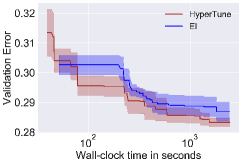
(a)

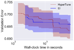
(b)

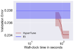
(c)

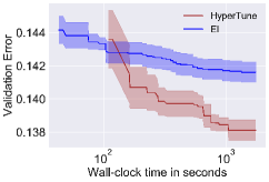
(d)

Figure 2: EI and HyperTune on validation dataset for Elastic net: (a) Letter, (b) MNIST, (c) Adult, and (d) Vehicle datasets.

Baselines	Average of the test error $\pm$ standard error
	Letter	MNIST	Adult	Vehicle
Fabolas	0.32$\pm$0.005	0.12$\pm$0.012	0.45$\pm$0.112	0.15$\pm$0.0005
HyperTune	0.3$\pm$0.000	0.11$\pm$0.007	0.24$\pm$0.000	0.14$\pm$0.0004

Table 1: Generalization performance on the heldout dataset for Elastic net.

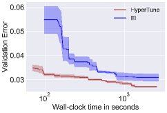
(a)

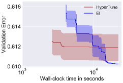
(b)

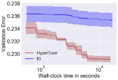
(c)

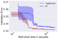
(d)

Figure 3: EI and HyperTune on validation dataset for SVM with RBF kernel: a) Letter, (b) MNIST, (c) Adult, and (d) Vehicle datasets.

Baselines	Average of the test error $\pm$ standard error
	Letter	MNIST	Adult	Vehicle
Fabolas	0.54$\pm$0.180	0.016$\pm$0.0005	0.24$\pm$0.0005	0.14$\pm$0.002
HyperTune	0.04$\pm$0.000	0.014$\pm$0.0002	0.24$\pm$0.0001	0.14$\pm$0.000

Table 2: Generalization performance on heldout dataset for SVM with RBF kernel.

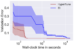
(a)

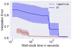
(b)

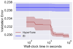
(c)

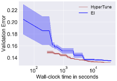
(d)

Figure 4: EI and HyperTune on validation dataset for SVM with kernel approximation: (a) Letter, (b) MNIST, (c) Adult, and (d) Vehicle datasets.

Baselines	Average of the test error $\pm$ standard error
	Letter	MNIST	Adult	Vehicle
Fabolas	0.09$\pm$0.014	0.076$\pm$0.03	0.242$\pm$0.000	0.18$\pm$0.016
Hyperband	0.04$\pm$0.002	0.019$\pm$0.00	0.246$\pm$0.002	0.137$\pm$0.000
HyperTune	0.03$\pm$0.000	0.018$\pm$0.00	0.242$\pm$0.000	0.138$\pm$0.000

Table 3: Generalization performance on heldout dataset for SVM with kernel approximation.

Experimental Results

Elastic Net

Elastic net is a logistic regression classifier with $L_{1}$ and $L_{2}$ penalty (?). The hyperparameters are the ratio parameter that trades-off $L_{1}$ and $L_{2}$ penalty, and the $\alpha$ parameter that determines the magnitude of the penalty. We tune the ratio parameter in the bound $[0,1]$. The penalty parameter $\alpha$ is tuned in an exponent space of $[-7,-1]$. In HyperTune, we assign a directional derivative sign $m=-1$ only for the hyperparameter $\alpha$ as the complexity of the model decreases with the penalty hyperparameter $\alpha$ while the other hyperparameter does not contribute to model complexity. The results for HyperTune and EI on the validation dataset are shown in 2. HyperTune outperforms EI in all the datasets. Table 2 reports the generalization performance of all the methods on a heldout dataset. HyperTune performs better than Fabolas in all cases.

SVM with RBF Kernel

In this experiment, we tune the cost parameter $C$ of SVM and the length-scale $\gamma$ of RBF kernel. We tune both the hyperparameters in an exponent space of $[-3,3]$. For HyperTune, we assign directional derivative signs $\mathbf{m}=\{1,1\}$ for both the hyperparameters $C$ and $\gamma$. The complexity of the model increases with an increase in both these hyperparameters. We compare the performance of EI and HyperTune on the validation dataset in Figure 3. In all the datasets, HyperTune significantly outperforms EI. We further record the generalization performance on the heldout dataset in Table 2. The results show that HyperTune again performs better than Fabolas, particularly in Letter dataset where the difference is significant.

SVM with Kernel Approximation using Random Fourier Features

In our third experiment, we tune the hyperparameters of SVM with kernel approximation using random Fourier features (?). We tune the cost parameter $C$, length-scale of RBF kernel $\gamma$ and the number of Fourier feature bases in this experiment. Both $C$, and $\gamma$ are tuned in the same bound as the previous experiment, and the number of Fourier features are tuned in an exponent space of $[3,12]$. We assign directional derivative signs $\mathbf{m}=\{1,1,1\}$ for all the hyperparameters since the model complexity increases with these hyperparameters. In Figure 4, we plot the results for HyperTune and EI on the validation dataset. HyperTune again outperforms EI in all the datasets. We also report the performance of the baselines on the heldout dataset in Table 3. The results show that HyperTune is either compatible or better than Hyperband. Both HyperTune and Hyperband outperform Fabolas in all the datasets except Adult dataset. Both Fabolas and HyperTune, however, perform better than Hyperband in Adult dataset.

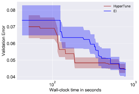
Figure 5: EI and HyperTune on validation dataset for MLP.

Baselines	Average of the test error $\pm$ standard error
	MLP on MNIST	CNN on CIFAR10
Fabolas	0.09$\pm$0.008	0.28
Hyperband	0.04$\pm$0.003	0.21
HyperTune	0.05$\pm$0.006	0.21

Table 4: Generalization performance on heldout dataset for MLP and CNN. We do not report the standard error for CNN as the experiment is conducted only once.

Multi-layer Perceptron

We tune five hyperparameters of an MLP on MNIST dataset. The hyperparameters here are the number of neurons, dropout, mini-batch size, learning rate, and momentum. We use stochastic gradient descent to learn the model. In this experiment, we assign $m=1$ only for the number of neurons in the hidden layers. We plot the results for EI and HyperTune on validation dataset in Figure 5. HyperTune performs better than EI on the validation dataset. We report the performance of the baselines on the heldout dataset in Table 4. Whilst Hyperband achieves the best performance in this experiment, HyperTune performs equally well. Both HyperTune and Hyperband perform better than Fabolas.

Convolutional Neural Network

We tune six hyperparameters of a CNN on benchmark real-world CIFAR10 dataset (?). Using the benchmark architecture configuration with 25 epochs, we tune batch size, dropout in the convolutional layers, learning rate, momentum, number of neurons in the fully connected layer, and dropout in the fully connected layer. For HyperTune, we use $m=1$ only for the number of neurons in the fully connected layer. We allocate a fixed a time budget of 24 hours to all the baselines and the best performance on the heldout dataset is reported in Table 4. Both Hyperband and HyperTune achieve the best generalization performance, and outperform Fabolas.

Conclusion

We have developed a fast hyperparameter tuning framework rooted in the insights from PAC learning theory. We have identified a novel way to leverage the trends in generalization performance from a subset of the data to the whole dataset. We have effectuated this using directional derivatives that signals the monotonic trends in the generalization performance of the models for hyperparameters which directly dictates model complexity. We evaluate the efficacy of our algorithm for tuning the hyperparameters of several machine learning algorithms on benchmark real-world datasets. The results demonstrate that our method is better than Fabolas (?) and the generic Bayesian optimization. We have also shown that HyperTune is compatible with the state-of-the-art hyperparameter tuning algorithm, Hyperband (?), and is widely applicable.

References

- [Kandasamy et al. 2017] Kandasamy, K.; Dasarathy, G.; Schneider, J.; and Póczos, B. 2017. Multi-fidelity Bayesian optimisation with continuous approximations. In Proceedings of the 34th International Conference on Machine Learning, volume 70 of Proceedings of Machine Learning Research, 1799–1808. PMLR.
- [Klein et al. 2017] Klein, A.; Falkner, S.; Bartels, S.; Hennig, P.; and Hutter, F. 2017. Fast Bayesian Optimization of Machine Learning Hyperparameters on Large Datasets. In Proceedings of the 20th International Conference on Artificial Intelligence and Statistics, volume 54 of Proceedings of Machine Learning Research, 528–536. PMLR.
- [Krizhevsky, Nair, and Hinton 2014] Krizhevsky, A.; Nair, V.; and Hinton, G. 2014. The cifar-10 dataset. online: http://www. cs. toronto. edu/kriz/cifar. html.
- [Li et al. 2017] Li, L.; Jamieson, K.; DeSalvo, G.; Rostamizadeh, A.; and Talwalkar, A. 2017. Hyperband: A novel bandit-based approach to hyperparameter optimization. In Proceedings of the International Conference on Learning Representations (ICLR 17).
- [Mockus, Tiesis, and Zilinskas 1978] Mockus, J.; Tiesis, V.; and Zilinskas, A. 1978. The application of Bayesian methods for seeking the extremum. Towards Global Optimization 2(117-129):2.
- [Rahimi and Recht 2007] Rahimi, A., and Recht, B. 2007. Random features for large-scale kernel machines. In Advances in Neural Information Processing Systems, 1177–1184.
- [Rasmussen et al. 2003] Rasmussen, C. E.; Bernardo, J.; Bayarri, M.; Berger, J.; Dawid, A.; Heckerman, D.; Smith, A.; and West, M. 2003. Gaussian processes to speed up hybrid monte carlo for expensive bayesian integrals. In Bayesian Statistics 7, 651–659.
- [Riihimäki and Vehtari 2010] Riihimäki, J., and Vehtari, A. 2010. Gaussian processes with monotonicity information. In Proceedings of the Thirteenth International Conference on Artificial Intelligence and Statistics, 645–652.
- [Shahriari et al. 2016] Shahriari, B.; Swersky, K.; Wang, Z.; Adams, R. P.; and de Freitas, N. 2016. Taking the human out of the loop: A review of bayesian optimization. Proceedings of the IEEE 104(1):148–175.
- [Snoek, Larochelle, and Adams 2012] Snoek, J.; Larochelle, H.; and Adams, R. P. 2012. Practical Bayesian optimization of machine learning algorithms. In Advances in Neural Information Processing Systems, 2951–2959.
- [Solak et al. 2003] Solak, E.; Murray-Smith, R.; Leithead, W. E.; Leith, D. J.; and Rasmussen, C. E. 2003. Derivative observations in gaussian process models of dynamic systems. In Advances in neural information processing systems, 1057–1064.
- [Swersky, Snoek, and Adams 2013] Swersky, K.; Snoek, J.; and Adams, R. P. 2013. Multi-task bayesian optimization. In Advances in Neural Information Processing Systems, 2004–2012.
- [Vanschoren et al. 2014] Vanschoren, J.; Van Rijn, J. N.; Bischl, B.; and Torgo, L. 2014. Openml: networked science in machine learning. ACM SIGKDD Explorations Newsletter 15(2):49–60.
- [Vapnik 1999] Vapnik, V. N. 1999. An overview of statistical learning theory. IEEE transactions on neural networks 10(5):988–999.
- [Williams and Rasmussen 2006] Williams, C. K., and Rasmussen, C. E. 2006. Gaussian processes for machine learning. the MIT Press 2(3):4.
- [Zou and Hastie 2005] Zou, H., and Hastie, T. 2005. Regularization and variable selection via the elastic net. Journal of the Royal Statistical Society: Series B (Statistical Methodology) 67(2):301–320.