Graph Approach to Extended Contextuality

Abstract

Exploring the graph approach, we restate the extended definition of noncontextuality provided by the contextuality-by-default framework. This extended definition avoids the assumption of nondisturbance, which states that whenever two contexts overlap, the marginal distribution obtained for the intersection must be the same. We show how standard tools for characterizing contextuality can also be used in this extended framework for any set of measurements and, in addition, we also provide several conditions that can be tested directly in any contextuality experiment. Our conditions reduce to traditional ones for noncontextuality if the nondisturbance assumption is satisfied.

I Introduction

Quantum theory provides a set of rules to predict probabilities of different outcomes in different experimental settings. Quantum predictions match with extreme accuracy the data from actually performed experiments Hensen et al. (2015); Giustina et al. (2015); Hensen et al. (2016); Ma et al. (2012); Boschi et al. (1998); Walborn et al. (2002); Lahiri et al. (2015), nonetheless they exhibit some peculiar properties deviating from the usual probabilistic description of classical systems Hardy (1993); Bell (1966, 1964). One of these “strange” characteristics is the phenomenon of contextuality, which says that there may be no global probability distribution over a set of measurements consistent with the quantum theory recovering the right prediction for each context, i.e. subsets of compatible measurements. Specker (1960); Bell (1966); Kochen and Specker (1967); Fine (1982); Abramsky and Brandenburger (2011).

A fundamental consequence of contextuality is that the statistical predictions of quantum theory cannot be obtained from models where measurement outcomes reveal pre-existent properties that are independent on other compatible measurements that are jointly performed Kochen and Specker (1967); Bell (1966). This limitation is related to the existence of incompatible measurements in quantum systems and thus represents an intrinsically non-classical phenomenon. Besides its importance for a more fundamental understanding of many aspects of quantum theory Nawareg et al. (2013); Cabello (2013a, b); Cabello et al. (2014); Amaral et al. (2014); Amaral (2014), contextuality has also been recognized as a potential resource for quantum computing, Raussendorf (2013); Howard et al. (2014); Delfosse et al. (2015), random number certification Um et al. (2013), and several other information processing tasks in the specific case of space-like separated systems Brunner et al. (2013).

As a consequence, experimental verifications of contextuality have attracted much attention Hasegawa et al. (2006); Kirchmair et al. (2009); Amselem et al. (2009); Lapkiewicz et al. (2011); Borges et al. (2014) over the past years. It is thus of utmost importance to develop a robust theoretical framework for contextuality that can be efficiently applied to real experiments. In particular, it is important to design a sound theoretical machinery well-adapted to cases in which the sets of measurements do not satisfy the assumption of nondisturbance Nawareg et al. (2013). This strong assumption demands that whenever the intersection of two contexts is non-empty, then the marginal probability distributions for the intersection must be the same, a restriction that will hardly be perfectly satisfied in real experiments.

In Refs. Kujala et al. (2015); Dzhafarov and Kujala (2016); Dzhafarov et al. (2016); Dzhafarov and Kujala (2017); Dzhafarov et al. (2017), the authors propose an alternative definition of noncontextuality, called contextuality-by-default or extended contextuality, that can be applied to any set of measurements. In this alternative definition, a set of measurements is said to be noncontextual (in the extended sense) if there is an extended joint probability distribution which is consistent with the joint distribution for each context and, in addition, maximizes the probability of two realizations of the same measurement in different contexts being equal. Such a treatment reduces to the traditional definition of noncontextuality if the nondisturbance property is satisfied and, in addition, it can be verified directly from experimental data. Finally, in Refs. Kujala et al. (2015); Kujala and Dzhafarov (2016) the authors provide necessary and sufficient conditions for extended contextuality in a broad class of scenarios, namely the $n$-cycle scenarios.

Focusing on developing an experimentally-friendly and robust theoretical framework for addressing noncontextuality, this contribution explores the graph approach to contextuality, developed in Refs. Cabello et al. (2010, 2014); Avis et al. (2006) and further explored in Refs. Rabelo et al. (2014); Acín et al. (2015); Amaral and Cunha (2017a), to rewrite the definition of extended contextuality in graph-theoretical terms. To this end, from the compatibility graph $\mathrm{G}$ of a scenario $\Gamma$, we define another graph $\mathscr{G}$ –the extended compatibility graph of the scenario– and show that extended noncontextuality is equivalent to noncontextuality in the traditional sense with respect to the extended graph $\mathscr{G}$. Within this graph-theoretical perspective, the problem of characterizing extended noncontextuality reduces to characterizing traditional noncontextuality for the scenario defined by $\mathscr{G}$, a difficult problem for general graphs Pitowsky (1991); Deza and Laurent (1997); Avis et al. (2006, 2008). Nevertheless, the graph-theoretic approach we employ here allows one to use several tools already developed for the study of contextuality also in the the characterization of extended contextuality.

We have organized the paper as follows: in Sec. II we review the definition of a compatibility scenario and of noncontextuality in the traditional sense. In Sec. III, we review the definition of extended noncontextuality as given in Refs. Kujala et al. (2015); Dzhafarov and Kujala (2016); Dzhafarov et al. (2016); Dzhafarov and Kujala (2017); Dzhafarov et al. (2017); Amaral et al. (2018a), stating it in graph-theoretical terms. We define the corresponding extended scenario and show that the notion of contextuality is equivalent to traditional contextuality with respect to the extended scenario. In Sec. IV we review several tools for the characterization of contextuality that can also be applied to the extended framework. In Sec. V we discuss different approaches to extended contextuality and argue why we believe the one proposed in Refs. Kujala and Dzhafarov (2016); Kujala et al. (2015) is more suitable. We finish this work with a discussion in Sec. VI.

II Compatibility scenarios

A compatibility scenario is defined by a triple

$$\Gamma:=\left(X,\mathcal{C},O\right),$$ (1)

where $O$ is a finite set, $X$ is a finite set representing measurements in a physical system whose possible outcomes lie in $O$, and $\mathcal{C}$ is a family of subsets of $X$. The elements $C\in\mathcal{C}$ are called contexts and encode the compatibility relations among the measurements in $X$, that is, each set $C\in\mathcal{C}$ consists of a maximal set of compatible, jointly measurable measurements Abramsky and Brandenburger (2011); Amaral and Cunha (2017b).

Equivalently, the compatibility relations among the elements of $X$ can be represented by a hypergraph. The compatibility hypergraph associated with a scenario $\left(X,\mathcal{C},O\right)$ is a hypergraph

$$\mathrm{H}:=\left(X,\mathcal{C}\right)$$ (2)

whose vertices are the measurements in $X$ and whose hyperedges are the contexts $C\in\mathcal{C}$.

When a particular set of compatible measurements in a context $C=\{x_{1},x_{2},...,x_{|C|}\}\in\mathcal{C}$ is performed jointly, a list $a=(a_{1},a_{2},...,a_{|C|})$ of outcomes in $O^{C}:=O\times O\times...\times O$ must be observed. The probability of this list of outcomes, with respect to this specific context, is denoted by

$$p\left(a|C\right)\coloneqq p\left(a_{1},\ldots,a_{|C|}\left|x_{1},\ldots,x_{|C|}\right.\right).$$ (3)

The collection of all these joint probability distributions is usually called Navascués et al. (2008); Junge et al. (2011) a behavior $\mathrm{B}$ for the scenario $\left(X,\mathcal{C},O\right)$.

In an ideal situation, it is generally assumed that behaviors must satisfy the nondisturbance condition Amaral (2014). Such condition says that whenever two contexts $C$ and $C^{\prime}$ overlap, the marginals for $C\cap C^{\prime}$, computed either from the distribution for $C$ or from the distribution for $C^{\prime}$, must coincide. The set of nondisturbing behaviors will be denoted by $\mathcal{ND}\left(\Gamma\right)$.

In the hypothetical situation where all measurements in $\mathrm{X}$ are compatible, i.e. in the extreme situation where there is a unique context, it would be possible to define a global probability distribution

$$p(a_{1}a_{2}...a_{|X|}|x_{1}x_{2}...x_{|X|})$$ (4)

dictating the probability of outcomes $a_{1}a_{2}...a_{|X|}$ in a joint measurement involving all measurements in $X$.

It is in a less extreme situation that the concept of (non)contextuality plays its role, though. A behavior $\mathrm{B}$ is noncontextual whenever the probability distributions assigned by $\mathrm{B}$ to each context can be recovered as marginals from a global probability distribution $p\left(a_{1}a_{2}\ldots a_{|X|}|x_{1}x_{2}...x_{|X|}\right)$ Fine (1982); Abramsky and Brandenburger (2011). The set of noncontextual behaviors will be denoted by $\mathcal{NC}\left(\Gamma\right)$. Notice that a noncontextual behavior is necessarily nondisturbing, what left us with the following inclusion

$$\mathcal{NC}\left(\Gamma\right)\subset\mathcal{ND}\left(\Gamma\right).$$ (5)

As an example, consider the scenario $\Gamma$ containing three dicotomic measurements $\{x,y,z\}$ where only one measurement, say $\{y\}$, is compatible with the two others. Mathematically, $\Gamma=\left(X,\mathcal{C},O\right)$ with ${O}=\left\{-1,1\right\}$, $\mathrm{X}=\left\{x,y,z\right\}$ and $\mathcal{C}=\left\{\{x,y\},\{y,z\}\right\}$. The compatibility hypergraph of this scenario is a simple graph , as depicted in Fig. 1.

Figure 1: A compatibility scenario with three measurements $x,y,z$ and two contexts, $\left\{x,y\right\}$ and $\left\{y,z\right\}$.

In this scenario, a behavior consists in specifying probability distributions

$$p(ab|xy),\,\,a,b\in\{-1,1\}$$ (6)

$$p(bc|yz),\,\,b,c\in\{-1,1\}.$$ (7)

The nondisturbance condition demands that

$$p\left(b|y\right)\coloneqq\sum_{a}p\left(ab|xy\right)=\sum_{c}p\left(bc|yz\right).$$ (8)

A behavior is noncontextual if there is a global probability distribution $p\left(abc|xyz\right)$ such that

$$p\left(ab|xy\right) =\sum_{c}p\left(abc|xyz\right)$$ (9)

$$p\left(bc|yz\right) =\sum_{a}p\left(abc|xyz\right).$$ (10)

III Extended Contextuality

To define noncontextuality in a scenario where the nondisturbance property does not hold true, we shall first consider extended global probability distributions of the form

$$p\left(\underbrace{a^{1}_{1}\ldots a^{1}_{\left|C_{1}\right|}}_{C_{1}}\underbrace{a^{2}_{1}\ldots a^{2}_{\left|C_{2}\right|}}_{C_{2}}\ldots\underbrace{a^{m}_{1}\ldots a^{m}_{\left|C_{m}\right|}}_{C_{m}}\left|\underbrace{x^{1}_{1}\ldots x^{1}_{\left|C_{1}\right|}}_{C_{1}}\underbrace{x^{2}_{1}\ldots x^{2}_{\left|C_{2}\right|}}_{C_{2}}\ldots\underbrace{x^{m}_{1}\ldots x^{m}_{\left|C_{m}\right|}}_{C_{m}}\right.\right),$$ (11)

where $m=\left|\mathcal{C}\right|$, that gives the joint probability of obtaining outcomes $a^{i}_{1},\ldots,a^{i}_{\left|C_{i}\right|}$ for each context $C_{i}=\left\{x^{i}_{1},\ldots,x^{i}_{\left|C_{i}\right|}\right\}.$ Notice that this extended global probability distribution is, in general, not equal to the probability distribution defined in Eq. (4), since the same measurement may appear in more than one context, and hence, in the list

$$\underbrace{x^{1}_{1}\ldots x^{1}_{\left|C_{1}\right|}}_{C_{1}}\underbrace{x^{2}_{1}\ldots x^{2}_{\left|C_{2}\right|}}_{C_{2}}\ldots\underbrace{x^{m}_{1}\ldots x^{m}_{\left|C_{m}\right|}}_{C_{m}}$$ (12)

the same measurement may be repeated several times.

To make definitions in Eqs.(4) and (11) equivalent in the case of nondisturbing behaviors, we demand that, if in different contexts $C_{i_{1}},C_{i_{2}},\ldots,C_{i_{l}}$ there exist coincident measurements $x^{i_{1}}_{k_{1}},x^{i_{2}}_{k_{2}},\ldots,x^{i_{l}}_{k_{l}}$ , then the marginal probability distributions for $x^{i_{1}}_{k_{1}},x^{i_{2}}_{k_{2}},\ldots,x^{i_{l}}_{k_{l}}$ are perfectly correlated. It is then equivalent to say that $\mathrm{B}$ is a noncontextual behavior if there is a extended global probability distribution satisfying this condition such that the marginals for each context coincide with the probability distributions of $\mathrm{B}$.

Consider the example framed in Fig.1. Traditionally, see Eq.(8), one says that a nondisturbing behavior for this scenario is noncontextual if there is a global probability distribution $p(abc|xyz)$ such that $p(ab|xy)=\sum_{c}p(abc|xyz)$ and $p(bc|yz)=\sum_{a}p(abc|xyz)$. An extended global probability distribution is a probability distribution $p(ab^{1}b^{2}c|xy^{1}y^{2}z)$ such that

$$p(b^{1}b^{2}|y^{1}y^{2}) = \sum_{a,c}p(ab^{1}b^{2}c|xy^{1}y^{2}z)$$

$$= \begin{cases}1&\text{if}\ b^{1}=b^{2}\\ 0&\text{otherwise}\end{cases},$$ (13)

where $y^{1}$ and $y^{2}$ represent the two copies of measurement $y$, one for each context. Then we say that a behavior is noncontextual if there is an extended global probability distribution satisfying condition (13) such that

$$p(ab^{1}|xy^{1})= \sum_{b^{2},c}p(ab^{1}b^{2}c|xy^{1}y^{2}z)$$ (14)

$$p(b^{2}c|y^{2}z)= \sum_{a,b^{1}}p(ab^{1}b^{2}c|xy^{1}y^{2}z).$$ (15)

For nondisturbing behaviors, these two notions of noncontextualtiy are equivalent Amaral et al. (2018a).

To define noncontextuality in a scenario where the nondisturbance property does not hold, we adopt the strategy of Refs. Kujala et al. (2015); Dzhafarov and Kujala (2016); Dzhafarov et al. (2016); Dzhafarov and Kujala (2017); Dzhafarov et al. (2017). That is to say, we relax the requirement that marginals for variables $x^{i_{1}}_{k_{1}},x^{i_{2}}_{k_{2}},\ldots,x^{i_{l}}_{k_{l}}$ must be perfectly correlated when they represent the same measurement. Instead, we require that the probability of $x^{i_{1}}_{k_{1}},x^{i_{2}}_{k_{2}},\ldots,x^{i_{l}}_{k_{l}}$ being equal is the maximum allowed by the individual probability distributions of each $x^{i_{l}}_{k_{l}}$.

We say that a behavior has a maximally noncontextual description if there is an extended global distribution (11) such that the distribution of each context is obtained as a marginal and such that if $x^{i_{1}}_{k_{1}},x^{i_{2}}_{k_{2}},\ldots,x^{i_{l}}_{k_{l}}$ represent the same measurement, the joint marginal distribution for $x^{i_{1}}_{k_{1}},x^{i_{2}}_{k_{2}},\ldots,x^{i_{l}}_{k_{l}}$ is such that

$$p\left(x^{i_{1}}_{k_{1}}=\ldots=x^{i_{l}}_{k_{l}}\right)=\sum_{a}p\left(a\ldots a\left|x^{i_{1}}_{k_{1}}\ldots x^{i_{l}}_{k_{l}}\right.\right)$$ (16)

is the maximum consistent with the marginal distributions $p\left(a^{i_{j}}_{k_{j}}\left|x^{i_{j}}_{k_{j}}\right.\right)$. In plain English, a behavior is noncontextual in the extended sense if there is an extended global distribution that gives the correct marginal in each context and that maximizes the probability of $x^{i_{1}}_{k_{1}},x^{i_{2}}_{k_{2}},\ldots,x^{i_{l}}_{k_{l}}$ being equal if they represent the same measurement in different contexts.

Given $\{x_{i_{1}}^{k_{1}},x_{i_{2}}^{k_{2}},\ldots,x_{i_{l}}^{k_{l}}\}$ representing the same measurement, we call a distribution

$$p\left(a_{i_{1}}^{k_{1}}a_{i_{2}}^{k_{2}}\ldots a_{i_{l}}^{k_{l}}\left|x_{i_{1}}^{k_{1}}x_{i_{2}}^{k_{2}}\ldots x_{i_{l}}^{k_{l}}\right.\right)$$ (17)

that gives the correct marginals $p\left(a_{i_{j}}^{k_{j}}\left|x_{i_{j}}^{k_{j}}\right.\right)$ a coupling for $x_{i_{1}}^{k_{1}},x_{i_{2}}^{k_{2}},\ldots,x_{i_{l}}^{k_{l}}$. We say that such a coupling is maximal if $p\left(x_{i_{1}}^{k_{1}}=x_{i_{2}}^{k_{2}}=\ldots=x_{i_{l}}^{k_{l}}\right)$ achieves the maximum value consistent with the marginals $p\left(a_{i_{j}}^{k_{j}}\left|x_{i_{j}}^{k_{j}}\right.\right)$.

Although maximal couplings always exist, as shown in Ref. Amaral et al. (2018a), there is no guarantee that they are unique. Nonetheless, there are specific scenarios – such as scenarios with two variables with any number of outcomes and three variables each of which with two outcomes– in which one can guarantee that this is indeed the case Amaral et al. (2018a).

Coming back once again to the example presented in Fig. 1, we say that a behavior is noncontextual in the extended sense if there is an extended global distribution

$$p\left(ab^{1}b^{2}c|xy^{1}y^{2}z\right)$$ (18)

such that

$$p\left(ab^{1}|xy^{1}\right)= \sum_{b^{2},c}p\left(ab^{1}b^{2}c|xy^{1}y^{2}z\right)$$ (19)

$$p\left(b^{2}c|y^{2}z\right)= \sum_{a,b^{1}}p\left(ab^{1}b^{2}c|xy^{1}y^{2}z\right)$$ (20)

and

$$p\left(y^{1}=y^{2}\right) \coloneqq\sum_{b}p\left(bb|y^{1}y^{2}\right)$$

$$=\sum_{a,b,c}p\left(abbc|xy^{1}y^{2}z\right)$$ (21)

is maximal with respect to the marginals

$$p\left(b^{1}|y^{1}\right)= \sum_{a}p\left(ab^{1}|xy^{1}\right)$$ (22)

$$p\left(b^{2}|y^{2}\right)= \sum_{c}p\left(b^{2}c|y^{2}z\right).$$ (23)

III.1 Extended compatibility scenario

To build a toolbox for extended contextuality, we associate to any scenario $\Gamma=\left(X,\mathcal{C},O\right)$ an extended scenario

$$\Upsilon\coloneqq\left(\mathscr{X},\mathscr{C},O\right),$$ (24)

constructed in the following way: to each vertex $x\in X$, let $C_{i_{1}},\ldots,C_{i_{l}}$ be all contexts containing it. The set $\mathscr{X}$ consists of measurements denoted by $x^{i_{1}},\ldots,x^{i_{l}}$, which represent different copies of the measurement $x$, one for each context containing it. For each $x\in X$ the set $\left\{x^{i_{1}},\ldots,x^{i_{l}}\right\}$ belongs to $\mathscr{C}$. The other contexts in $\mathscr{C}$ are in one-to-one correspondence with the contexts in $\mathcal{C}$: each context $C_{i}=\left\{x_{1},x_{2},\ldots,x_{\left|C_{i}\right|}\right\}$ in $\mathcal{C}$ corresponds the context $\left\{x_{1}^{i},x_{2}^{i},\ldots,x_{\left|C_{i}\right|}^{i}\right\}$ in $\mathscr{C}$. The extended compatibility hypergraph $\mathscr{H}$ of the scenario is the compatibility hypergraph of the extended scenario $\Upsilon$.

Fig. 2 illustrates the extended compatibility hypergraph of the scenario defined in Fig. 1. In this scenario we have three measurements $x,y,z$ and two contexts, $C_{1}=\left\{x,y\right\}$ and $C_{2}=\left\{y,z\right\}$. Measurement $x$ belongs only to context $C_{1}$, measurement $z$ belongs only to context $C_{2}$, while measurement $y$ belongs to both contexts. Hence, $\mathscr{X}=\left\{x^{1},y^{1},y^{2},z^{2}\right\}$. The contexts in $\mathscr{C}$ are $\left\{y^{1},y^{2}\right\}$, $\left\{x^{1},y^{1}\right\}$ and $\left\{y^{2},z^{2}\right\}$, the last two being the ones corresponding to those of $\mathcal{C}$. Since $x$ and $z$ have only one copy in $\mathscr{X}$ we continue denoting these measurements simply by $x$ and $z$.

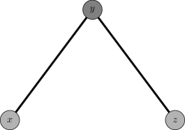
(a)

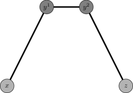
(b)

Figure 2: (a) Compatibility hypergraph $\mathrm{H}$ of Fig. 1. (b) The extended compatibility hypergraph $\mathscr{H}$ of $\mathrm{H}$.

Given a behavior $\mathrm{B}$ for $\Gamma$, we construct an extended behavior $\mathscr{B}$ for $\mathrm{B}$ in the following way: for each context $\left\{x_{1}^{i}x_{2}^{i}\ldots x_{\left|C_{i}\right|}^{i}\right\}$ of $\mathscr{C}$ corresponding to context $C_{i}=\left\{x_{1}x_{2}\ldots x_{\left|C_{i}\right|}\right\}$ of $\mathcal{C}$ the probability distribution assigned by behavior $\mathscr{B}$ is equal to the probability distribution assigned to $C_{i}$ via the original behavior $\mathrm{B}$; for context $x^{i_{1}},\ldots,x^{i_{l}}$ of $\mathscr{C}$ corresponding to the different copies of a measurement $x\in X$, the probability distribution assigned by behavior $\mathscr{B}$ is any maximal coupling for the variables $x^{i_{1}},\ldots,x^{i_{l}}$. Since, in general, maximal couplings are not unique, $\mathscr{B}$ will also not be unique.

In the example of Fig. 1, a behavior $B$ corresponds to two probability distributions $p\left(ab|xy\right)$ and $p\left(bc|yz\right)$. An extended behavior $\mathscr{B}$ corresponds to three probability distributions $p\left(ab^{1}|xy^{1}\right)$, $p\left(b^{2}c|y^{2}z\right)$ and $p\left(b^{1}b^{2}|y^{1}y^{2}\right)$, such that the distribution for $xy^{1}$ is the same as the distribution for $xy$, the distribution for $y^{2}z$ is the same as the distribution for $yz$ and $p\left(b^{1}b^{2}|y^{1}y^{2}\right)$ maximizes the probability of $y^{1}$ and $y^{2}$ being equal given the marginals $p\left(b^{1}|y^{1}\right)$ and $p\left(b^{2}|y^{2}\right)$.

In Ref. Dzhafarov and Kujala (2017), the authors define the notion of multimaximal coupling and use this notion to give a different definition of extended contextuality. In this work we prefer to adopt maximal couplings as our starting point and by doing so we point out and discuss in details the differences between both approaches in Sec. V. We notice, however, that the tools used here apply to both cases, and, more generally, to any kind of coupling one imposes on the sets $x^{i_{1}},\ldots,x^{i_{l}}$ of $\mathscr{C}$. Physical constraints shall ultimately decide which couplings are more meaningful. Once the relevant couplings are defined, the notion of extended behavior will follow analogously and the mathematics from this step forward is exactly the same in all situations.

With these concepts in hands, we can rewrite the definition of extended contextuality as the following theorem:

Theorem 1.

A behavior $\mathrm{B}$ for $\Gamma$ has a maximally noncontextual description if, and only if, there is an extended behavior $\mathscr{B}$ for $\mathrm{B}$ which is noncontextual in the traditional sense with respect to the extended scenario $\Upsilon$.

Thus, the problem of deciding whether a behavior $\mathrm{B}$ is noncontextual in the extended sense is equivalent to the problem of finding an extended behavior $\mathscr{B}$ which is noncontextual in the extended scenario $\Upsilon$. Hence, the tools needed for the characterization of extended contextuality in the contextuality-by-default framework are exactly the same tools used in the characterization of contextuality in the traditional definition, with the complication that the scenario under study is more complex and that one may have to look to several different extended behaviors.

This gives, as corollary, a complete characterization of extended contextuality for the $n$-cycle scenario Kujala et al. (2015); Kujala and Dzhafarov (2016); Amaral et al. (2018a). In the $n$-cycle scenario, $X=\left\{0,\ldots,n-1\right\}$ and two measurements $i$ and $j$ are compatible iff $j=i+1\mod n$. The corresponding hypergraph $\mathrm{H}$ is the cycle $\mathrm{C}_{n}$ with $n$ vertices. The extended hypergraph $\mathscr{H}$ is a $2n$-cycle, with vertices $i^{i},i^{i+1}$ and egdes $\left\{i^{i},(i+1)^{i}\right\},\left\{i^{i},i^{i-1}\right\},\ i=0,\ldots,n-1$ (see Fig. 3).

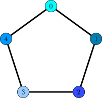
(a)

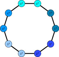
(b)

Figure 3: (a) The compatibility hypergraph $\mathrm{H}$ of the $5$-cycle scenario, which consists of five measurements $0,\ldots,4$ and five contexts $\left\{i,i+1\right\}$, $i=0,\ldots,4$, the sum being taken $\mod 5$. (b) The extended compatibility hypergraph $\mathscr{H}$ of the $5$-cycle scenario, which is a $10$-cycle with vertices $i^{i-1},i^{i}$ and egdes $\left\{i^{i},(i+1)^{i}\right\},\left\{i^{i},i^{i-1}\right\},\ i=0,\ldots,4$.

Corollary 2.

A behavior $B$ for the $n$-cycle scenario is noncontextual in the extended sense iff

$$s\left(\left\langle{i}^{i}(i+1)^{i}\right\rangle,1-\left|\left\langle i^{i}\right\rangle-\left\langle i^{i-1}\right|\right\rangle\right)_{i=0,\ldots,n-1}$$

$$\leq 2n-2,$$ (25)

where

$$s\left(z_{1},\ldots,z_{k}\right)=\max_{\gamma_{i}=\pm 1,\prod_{i}\gamma_{i}=-1}\sum_{i=1}^{k}\gamma_{i}z_{i}.$$ (26)

In fact, the extended behavior $\mathscr{b}$ is unique and, as shown in Ref. Kujala et al. (2015), for every context $\left\{i^{i-1},i^{i}\right\}$ corresponding to $i\in X$ we have that the maximal coupling satisfy:

$$\left\langle i^{i-1}i^{i}\right\rangle=1-\left|\left\langle i^{i-1}\right\rangle-\left\langle i^{i}\right\rangle\right|.$$ (27)

As shown in Ref. Araújo et al. (2013), Eq. (25) is a necessary and sufficient condition for membership in the noncontextual set of the scenario defined by $\mathrm{C}_{2n}$ and the result follows from Thm. 1.

IV Necessary and Sufficient conditions for extended contextuality

In this section we list several tools developed for the characterization of traditional contextuality. As a consequence of Thm. 1, these tools can also be applied directly to the extended scenario to characterize extended contextuality in the contextuality-by-default framework.

IV.1 Testing Noncontextuality with Linear Programming

Noncontextuality of a behavior $\mathrm{B}$ is equivalent Amaral et al. (2018b) to the existence of a set of variables $\Lambda$ and deterministic probability distributions $p\left(a_{i}|x_{i},\lambda\right)$ for each $x_{i}\in X$ and $\lambda\in\Lambda$ such that

$$p\left(a_{1},\ldots,a_{\left|C\right|}|x_{1},\ldots,x_{\left|C\right|}\right)$$

$$= \sum_{\lambda}p(\lambda)\prod_{i=1}^{\left|C\right|}p\left(a_{i}|x_{i},\lambda\right).$$ (28)

It is possible to show that it suffices to consider a set $\Lambda$ with the same number of elements as the extremal points of the noncontextual set Schmid et al. (2018).

The most general way of deciding whether a behavior can be written in the form (28) is through a linear program (LP) formulation Dzhafarov and Kujala (2016). Representing each probability distribution as a vector, Eq.(28) can be written succinctly as

$$\mathrm{B}=A\cdot\bm{\lambda},$$ (29)

with $\bm{\lambda}$ being a vector with components

$$\lambda_{i}=p(\lambda=i)$$ (30)

and $A$ being a matrix whose columns are the deterministic distributions

$$\prod_{j=1}^{\left|C\right|}p\left(a_{j}|x_{j},\lambda_{i}\right),$$ (31)

that is, the columns of $A$ are the extremal points of the noncontextual set. Hence, checking whether $\mathrm{B}$ is noncontextual amounts to solve a simple feasibility problem written as the following LP :

$$\min_{\lambda\in\mathds{R}^{m}} \quad\quad\mathbf{v}\cdot\bm{\lambda}$$

subject to $$\quad\mathrm{B}=A\cdot\bm{\lambda}$$

$$\quad\lambda_{i}\geq 0$$

$$\quad\sum_{i}\lambda_{i}=1,$$

where $\mathbf{v}$ represents an arbitrary vector with the same dimension $m=|O|^{|X|}$ as the vector representing the variable $\bm{\lambda}$.

As a consequence of Thm. 1, we have:

Theorem 3.

A behavior $\mathrm{B}$ is noncontextual in the extended sense if there is an extended behavior $\mathscr{B}$ in the extended scenario such that the following linear program

$$\min_{\lambda\in\mathds{R}^{m}} \quad\quad\mathbf{v}\cdot\bm{\lambda}$$ (33)

subject   to $$\quad\mathscr{B}=\mathscr{A}\cdot\bm{\lambda}$$

$$\quad\lambda_{i}\geq 0$$

$$\quad\sum_{i}\lambda_{i}=1,$$

is feasible, where $\mathscr{A}$ is a matrix whose columns are products of extremal points of the noncontextual polytope of the extended scenario.

IV.2 Noncontextuality Inequalities

In a scenario $\Gamma=(X,\mathcal{C},O)$, given $\gamma_{s|C}$ and $\mathrm{b}\in\mathds{R}$ we say that the linear inequality

$$\sum_{s\in O^{\left|C\right|},C\in\mathcal{C}}\gamma_{s|C}p\left(s|C\right)\leq\mathrm{b},$$ (34)

is a noncontextuality inequality if it is satisfied for all $\mathrm{B}\in\mathcal{NC}\left(\Gamma\right)$.

Every noncontextuality inequality gives rise to a necessary condition for noncontextuality in the corresponding scenario. The noncontextual set is a polytope and hence it is characterized by a finite number of noncontextuality inequalities Amaral (2014). The complete characterization of the noncontextual set requires one to find all facet defining inequalities and this is in general a hard problem, specially in the extended framework where the number of measurements is large. Nevertheless, there are algorithms that can list all the facet-defining inequalities for small graphs.

For scenarios where the contexts have at most two measurements and each measurement has two outcomes, we can explore the connection between the noncontextual set and the cut polytope $\mathrm{CUT}\left(\mathrm{H}\right)$ Avis et al. (2006); Amaral and Cunha (2017a) of the corresponding compatibility hypergraph $\mathrm{H}$. In this case $\mathrm{H}$ is nothing but a simple graph and, if the nondisturbance condition is satisfied, deriving necessary conditions for extended contextuality reduces to the traditional necessary conditions for noncontextuality.

A detailed discussion of this connection is presented in Ref. Amaral et al. (2018a). There the authors have proven that the extended compatibility hypergraph $\mathscr{H}$ can be obtained from the compatibility hypergraph $\mathrm{H}$ combining graph operations known as triangular elimination, vertex splitting and edge contraction Barahona and Mahjoub (1986); Avis et al. (2008); Bonato et al. (2014). From valid inequalities for $\mathrm{CUT}\left(\mathrm{H}\right)$ it is possible to derive valid inequalities for any graph obtained from $\mathrm{H}$ using a sequence of such operations. In particular, for any valid inequality for $\mathrm{CUT}\left(\mathrm{H}\right)$ it is possible to derive valid inequalities for $\mathrm{CUT}\left(\mathscr{H}\right)$, among which there is one that reduces to the original inequality if the nondisturbance condition is satisfied. Hence, for every noncontextuality inequality in the traditional sense, we can derive a family of inequalities in the extended sense. Any violation of the inequalities obtained with this method implies that the extended behavior is contextual in the extended sense.

IV.3 Noncontextuality Quantifiers

Following the same reasoning we used above, extended noncontextuality of a behavior can also be witnessed with noncontextuality quantifiers, i.e. in order to define whether a given behavior is contextual we can also explore those functions associating each behavior $\mathrm{B}$ with a positive number $\mathrm{Q}\left(\mathrm{B}\right)$ such that $\mathrm{Q}\left(\mathrm{B}\right)=0$ if and only if $\mathrm{B}$ is noncontextual.

Once again, as a consequence of Thm. 1, we have:

Theorem 4.

A behavior $\mathrm{B}$ is noncontextual in the extended sense if and only if there is an extended behavior $\mathscr{B}$ such that $Q\left(\mathscr{B}\right)=0$ for some contextuality quantifier $Q$.

In what follows we exhibit a number of monotones of contextuality developed recently that can be used to witness extended contextuality in any scenario.

IV.3.1 Relative Entropy of Contextuality

The relative entropy of contextuality of a behavior $B$ Grudka et al. (2014); Horodecki et al. (2015) is defined as

$$E_{max}\left(B\right) :=$$

$$\min_{B^{NC}\in\mathcal{NC}\left(\Gamma\right)} \ \ \max_{C}\ \ D_{\mathrm{KL}}\left(p(\cdot|C)\middle\|p^{NC}(\cdot|C)\right),$$ (35)

where $p(\cdot|C)$ is the probability distribution given by the behavior $\mathrm{B}$ for context $C$, the minimum is taken over all noncontextual behaviors $B^{NC}=\left\{p^{NC}(\cdot|C)\right\}$ and the maximum is taken over all contexts $C\in\mathcal{C}$.

On the other hand, the uniform relative entropy of contextuality of $B$ is defined as

$$E_{u}\left(B\right) :=$$

$$\frac{1}{|\mathcal{C}|}\min_{B^{NC}\in\mathcal{NC}\left(\Gamma\right)} \ \ \sum_{C\in\mathcal{C}}\ D_{\mathrm{KL}}\left(p(\cdot|C)\middle\|p^{NC}(\cdot|C)\right),$$ (36)

where the minimum is taken over all noncontextual behaviors $B^{NC}=\left\{p^{NC}(\cdot|C)\right\}$.

Both $E_{max}$ and $E_{u}$ vanish if and only if $\mathrm{B}$ is noncontextual. In addition, while $E_{max}$ is a proper monotone in a resource theory of contextuality with noncontextual wirings as free-operations, the uniform relative entropy of contextuality is not. For more detailes, see Refs. Gallego and Aolita (2017); Amaral et al. (2018b).

IV.3.2 Distances

In Refs. Amaral and Cunha (2017a); Brito et al. (2018), the authors define contextuality monotones based on geometric distances, in contrast with the previous defined quantifiers which are based on entropic distances. Let $D$ be any distance defined in real vector space $\mathds{R}^{K}$. The $D$-contextuality distance of a behavior $B$ is defined as

$$\mathcal{D}\left(B\right):=\min_{\mathrm{B}^{NC}\in\mathcal{NC}\left(\Gamma\right)}D\left(\mathrm{B},\mathrm{B}^{NC}\right).$$ (37)

We can also calculate the distance between the behaviors $B$ and $B^{NC}$ for each context $C$ and then average over the contexts. When the choice of context is uniform, we have the $D$-uniform contextuality distance of a behavior $B$, defined as

$$\mathcal{D}_{u}\left(B\right) :=$$

$$\frac{1}{N}\min_{B^{NC}\in\mathcal{NC}\left(\Gamma\right)} \sum_{C\in\mathcal{C}}D\left(p(\cdot|C),p^{NC}(\cdot|C)\right),$$ (38)

where $N=\left|\mathcal{C}\right|$ is the number of contexts in $\mathcal{C}$, $p(\cdot|C)$ is the probability distribution given by the behavior $\mathrm{B}$ for context $C$, and the minimum is taken over all noncontextual behaviors $B^{NC}=\left\{p^{NC}(\cdot|C)\right\}$.

If we allow for non-uniform choices of context, the natural way of quantifying contextuality will be the $D$-max contextuality distance of a behavior $B$, defined as

$$\mathcal{D}_{max}\left(B\right) :=$$

$$\min_{B^{NC}\in\mathcal{NC}\left(\Gamma\right)} \max_{C}D\left(p(\cdot|C),p^{NC}(\cdot|C)\right),$$ (39)

where the minimum is taken over all noncontextual behaviors $B^{NC}=\left\{p^{NC}(\cdot|C)\right\}$ and the maximum is taken over all contexts $C\in\mathcal{C}$.

The quantifiers $\mathcal{D}$, $\mathcal{D}_{u}$ and $\mathcal{D}_{max}$ vanish if and only if $\mathrm{B}$ is noncontextual. The quantifier $\mathcal{D}_{max}$ is a proper monotone in a resource theory of contextuality based on noncontextual wirings if the distance $d$ comes from a $\ell_{p}$-norm in $\mathds{R}^{K}$. If we choose the $\ell_{1}$-norm, $\mathcal{D}_{u}$ can be efficiently computed using linear programming Amaral and Cunha (2017a). A detailed discussion of this quantifier for the special class of Bell scenarios can be found in Ref. Brito et al. (2018).

For the special class of $n$-cycle scenarios, the distance $\mathcal{D}_{u}$ defined with the $\ell_{1}$-norm is given by

$$\mathcal{D}_{u}\left(B\right):=\frac{1}{N}\min_{B^{NC}\in\mathcal{NC}\left(\Gamma\right)}\sum_{C\in\mathcal{C},a\in O^{C}}\left|p(a|C)-p^{NC}(a|C)\right|_{\ell_{1}}=\frac{1}{2}\max_{s}\left[s\left(\left\langle{i}^{i}(i+1)^{i}\right\rangle\right)-(n-2)\right],$$ (40)

where $s$ was defined in equation (26). This shows that for $n$-cycle scenarios, the distance $\mathcal{D}_{u}(B)$ defined by the $\ell_{1}$-norm is equal to the violation of the only noncontextual inequality (25) violated by $B$.

In the extended $n$-cycle scenario, there is only one extended behavior $\mathscr{B}$ for each behavior $B$. Hence, the quantifier in the extended sense will also be given by

$$\mathcal{D}_{u}\left(\mathscr{B}\right)=\frac{1}{2}\max_{s}\left[s\left(\left\langle{i}^{i}(i+1)^{i}\right\rangle,1-\left\langle i^{i}\right\rangle-\left\langle i^{i-1}\right\rangle\right)-(2n-2)\right]$$ (41)

and it will vanish if and only if $B$ is noncontextual in the extended sense.

IV.3.3 Contextual Fraction

Broadly speaking, we may interpret the contextual fraction of a behavior as a contextuality quantifier based on the intuitive notion of which fraction of it admits a noncontextual description. Such measure was introduced in Refs. Abramsky and Brandenburger (2011); Amselem et al. (2012), and several properties of this quantifier were further discussed in Ref. Abramsky et al. (2017).

More specifically, the contextual fraction of a behavior $B$ is defined as

$$\mathcal{CF}\left(B\right)=\min\left\{\lambda\left|B=\lambda B^{\prime}+\left(1-\lambda\right)B^{NC}\right.\right\},$$ (42)

where $B^{NC}$ is an arbitrary noncontextual behavior. The contextual fraction vanishes if and only if $\mathrm{B}$ is noncontextual and it can be efficiently computed using linear programming.

In the $n$-cycle scenario, each behavior $B$ violates only one facet-defining inequality (25). This implies that we can write

$$B=\mathcal{CF}\left(B\right)B^{\prime}+\left(1-\mathcal{CF}\left(B\right)\right)B^{NC}$$ (43)

where $B^{NC}$ is a noncontextual behavior saturating the inequality and $B^{\prime}$ is the only contextual behavior that maximally violates the inequality. The linearity of the noncontextuality inequalities in turn implies that $B$ will violated this inequality by $\mathcal{CF}\left(B\right)$ times the violation obtained with $B^{\prime}$. Hence, we also have that

$$\mathcal{CF}\left(B\right)=\frac{1}{n}\max_{s}\left[s\left(\left\langle{i}^{i}(i+1)^{i}\right\rangle,1-\left\langle i^{i}\right\rangle-\left\langle i^{i-1}\right\rangle\right)-(n-2)\right].$$ (44)

Clearly, and analogously to what we have done for the $D$-uniform contextuality distance, Eq. (44) will also hold true in the extended scenario.

IV.3.4 Negativity of global quasidistributions

A quasiprobability distribution is a set of real numbers $p_{i}$ such that $\sum_{i}p_{i}=1.$ If we relax the restriction that $p\left(a_{1}a_{2}\ldots a_{n}|x_{1}x_{2}...x_{|X|}\right)$ be a probability distribution and require only that it is be a quasiprobability distribution, then every nondisturbing behavior has a global quasiprobability distribution consistent with it Abramsky and Brandenburger (2011). Noncontextuality can be characterized in terms of these quasiprobability distributions: a behavior in noncontextual if and only if there is such global quasiprobability distribution with all $p\left(a_{1}a_{2}\ldots a_{n}|x_{1}x_{2}...x_{|X|}\right)\geq 0.$

We can also use these distributions to derive a contextuality quantifier

$$\mathrm{N}\left(\mathrm{B}\right)=\min\sum_{a,\mathrm{C}}\left|p\left(a_{1}a_{2}\ldots a_{\left|X\right|}|x_{1}x_{2}...x_{|X|}\right)\right|-1$$ (45)

where the minimum is taken over all global quasiprobability distributions consistent with $\mathrm{B}$ and the sum is taken over all contexts $\mathrm{C}=\left\{x_{1},x_{2},\ldots,x_{|X|}\right\}$ and all possible outcomes $a=\left(a_{1}a_{2}\ldots a_{\left|X\right|}\right)\in O^{\mathrm{C}}$. We have that $\mathrm{N}\left(\mathrm{B}\right)=0$ if and only if there is a global probability distribution consistent with $\mathrm{B}$, and hence $\mathrm{N}$ is indeed a proper contextuality quantifier. It can be calculated using linear programming, since the sum can be formulated as

$$\min_{\mathbf{t}\in\mathds{R}^{n},\lambda\in\mathds{R}^{m}} \langle\mathbf{1}_{n},\mathbf{t}\rangle$$ (46)

$$\mathrm{subjected\ to} \quad-\mathbf{t}\leq\mathrm{B}-A\cdot\lambda\leq\mathbf{t}$$

$$\quad\sum_{i}\lambda_{i}=1,$$

where $A$ is the matrix whose columns are the extremal points of the noncontextual polytope.

As a consequence of Thm.  1, $B$ is noncontextual in the extended sense if and only if there is an extended behavior $\mathscr{B}$ for $B$ such that $\mathrm{N}\left(\mathscr{B}\right)=0$. For $n$-cycle scenarios $\mathrm{N}\left(\mathscr{B}\right)$ is given by Dzhafarov and Kujala (2016)

$$\mathcal{N}\left(\mathscr{B}\right)=\frac{1}{2}\max_{s}\left[s\left(\left\langle{i}^{i}(i+1)^{i}\right\rangle,1-\left\langle i^{i}\right\rangle-\left\langle i^{i-1}\right\rangle\right)-(2n-2)\right].$$ (47)

IV.4 Difference between maximal couplings and extended global distributions

In Refs. Dzhafarov and Kujala (2017); Kujala and Dzhafarov (2016) the authors define a specific contextuality quantifier for the contextuality-by-default approach based on the fact that no extended global probability distribution consistent with the original behavior $\mathrm{B}$ can give a maximal coupling for the copies of all measurements $x\in X$ if $\mathrm{B}$ is contextual. Let $x^{1},\ldots,x^{n}$ be the different copies of a measurement $x\in X$. We define

$$\mathrm{\mu}\left(\mathrm{x}\right)=\max p\left(x^{1}=x^{2}=\ldots=x^{n}\right)$$ (48)

where the maximum is taken over all couplings of $x^{1},\ldots,x^{n}$, that is, $\mu(x)$ gives the probability of $x^{1},\ldots,x^{n}$ being equal according to any maximal coupling for $x^{1},\ldots,x^{n}$.

Given an extended global distribution $q$ we compute the probability of $x^{1},\ldots,x^{n}$ being equal according to $q$:

$$\mathrm{m}^{q}\left(\mathrm{x}\right)=q\left(x^{1}=x^{2}=\ldots=x^{n}\right).$$ (49)

Combining these two quantities, we define

$$\mathrm{M}_{u}\left(\mathrm{B}\right):=\sum_{x\in X}\mathrm{\mu}\left(\mathrm{x}\right)-\max_{q}\sum_{x\in X}\mathrm{m}^{q}\left(\mathrm{x}\right),$$ (50)

where the maximum is taken over all extended global distributions $q$ consistent with $\mathrm{B}$. Notice that $\mathrm{M}_{u}\left(\mathrm{B}\right)=0$ if and only if there is an extended global distribution consistent with some extended behavior $\mathscr{B}$ of $\mathrm{B}$, that is, if and only if $\mathrm{B}$ is noncontextual in the extended sense. This quantity can also be calculated using linear programming since it involves the maximization of the linear function

$$\sum_{x}m^{q}(x)$$ (51)

over the set of extended global distributions $q$ consistent with $B$ in each context $C$.

It turns out that this quantifier is related to the the violation of the noncontextuality inequalities (25) for the $n$-cycle scenarios. In fact, it was shown in Ref. Kujala and Dzhafarov (2016) that

$$\mathrm{M}_{u}\left(\mathrm{B}\right)=\frac{1}{2}\max\left\{s\left(\left\langle{i}^{i}(i+1)^{i}\right\rangle,1-\left|\left\langle i^{i}\right\rangle-\left\langle i^{i-1}\right|\right\rangle\right)_{i=0,\ldots,n-1}-(2n-2),0\right\}.$$ (52)

This proves that, for $n$-cycle scenarios, the quantifiers $\mathrm{M}_{u}$, $N$, $\mathcal{CF}$ and $\mathcal{D}_{u}$ defined with the $\ell_{1}$-norm are all equivalent. This is also true for $\mathcal{D}_{u}$ defined with any $\ell_{p}$-norm, as shown in Ref. Amaral and Cunha (2017a).

In references Auffèves and Grangie (2016); Amaral et al. (2018b) the authors show that the quantifiers $E_{u}$ and $D_{u}$ are not monotones under the entire set of noncontextual wirings, as some preprocessings of the measurement labels $x_{i}$ may increase these quantifiers in an artificial way using only noncontextual resources. This shows that taking sums or means over the contexts generally do not lead to proper contextuality quantifiers when the entire class of noncontextual wirings is to be considered. Although we still lack a resource theory for contextuality that can be applied to the contextuality-by-default framework, we expect the same problem to happen with the quantifier $\mathrm{M}_{u}$. It might be the useful then to take the maximum over measurements $x$ instead of the sum:

$$\mathrm{M}\left(\mathrm{B}\right)=\min_{q}\max_{x\in X}\left[\mathrm{\mu}\left(\mathrm{x}\right)-\mathrm{m}^{q}\left(\mathrm{x}\right)\right],$$ (53)

where the minimum is taken over all extended probability distributions $q$ consistent with $\mathrm{B}$. Notice that we also have that $\mathrm{M}\left(\mathrm{B}\right)=0$ if and only if $\mathrm{B}$ is noncontextual in the extended sense. Although possibly more suitable from the point of view of resource theories, this quantifier has the disadvantage of not being computed with linear programming. Nevertheless, for the special case of $n$-cycle scenario, $\mathrm{M}_{u}$ and $\mathrm{M}$ coincide. In fact, it is always possible to find an extended global distribution that agrees with $\mathscr{B}$ for all contexts except one.

V Different Couplings

Following Refs. Kujala et al. (2015); Dzhafarov et al. (2016), we defined extended contextuality using the notion of maximal coupling. This kind of coupling has the property that a maximal coupling for a set of variables is not necessarily a maximal coupling when we compute the marginal for a subset of these variables. Hence, a noncontextual behavior $\mathrm{B}$ might become contextual in the extended sense when some measurements are ignored Dzhafarov and Kujala (2017).

In Ref. Dzhafarov and Kujala (2017) the authors regard this property as a disadvantage of this kind of coupling and replace the constraint of maximal coupling by the constraint of multimaximal coupling. A multimaximal coupling for a set of variables $x_{1},\ldots,x_{n}$ is a maximal coupling for $x_{1},\ldots,x_{n}$ such that if we compute the marginal distribution for every subset of $x_{1},\ldots,x_{n}$, the resulting distribution is also a maximal coupling for this subset. The main disadvantage of this kind of constraint is that depending on the marginals for $x_{1},\ldots,x_{n}$ this kind of coupling may not exist.

Our main motivation to study extended contextuality comes from the need of developing a formal structure for contextuality that can be applied to any experiment. Hence, the multimaximal coupling constraint is not a good choice for this particular application since there is no guarantee that such a coupling exists for every experimental data. On the other hand, the fact that a maximal coupling for a set of variables is not necessarily a maximal coupling when we compute the marginal for a subset of these variables can be intuitively explained in this situation. Imagine that a measurement $x$ appears in four different contexts. In the extended scenario this measurement will correspond to four variables $x^{1},x^{2},x^{3},x^{4}$. Suppose that the measurement of the first two contexts is perfect and the measurement of the last two contexts has a lot of errors. It is possible that, even if you start with a setting that should in theory exhibit contextuality, the data will be noncontextual in the extended sense if the measurements of the last two contexts are really bad. Hence, discarding these contexts will leave only the contexts where the measurement is perfect, and hence the data may become contextual. Errors contribute to make the experimental behaviors noncontextual and it might be the case that discarding some measurements where the data is worse will make the behavior contextual in the smaller scenario.

We stress that the tools listed in Sec. IV will work for any choice of coupling for the copies of the same measurement one chooses. We believe that this choice may depend on the application and it is important to debate which choice is the most appropriate in each situation. The generalization of contextuality provided by this framework can lead to a better comprehension of the data in contextuality experiments without unreal idealizations, but we believe that the kind of coupling one should impose needs to be further discussed. Particularly, we should investigate if it is possible to justify the use of a specific coupling with experimental data. Nevertheless, once the choice is made the notion of extended behavior will follow analogously and the mathematics from this step forward is exactly the same in all situations.

VI Discussion

Apart from its primal importance in the foundations of quantum physics, contextuality has been discovered as a potential resource for quantum computing Raussendorf (2013); Howard et al. (2014); Delfosse et al. (2015), random number certification Um et al. (2013), and several other tasks in the particular case of Bell scenarios Brunner et al. (2013). Within these both fundamental and applied perspectives, certifying contextuality experimentally is undoubtedly an important primitive. It is then crucial to develop a robust theoretical framework for contextuality that can be easily applied to real experiments. This should include the possibility of treating sets of measurements that do not satisfy the assumption of nondisturbance, which will be hardly satisfied in experimental implementations Kujala et al. (2015).

It is in the pursuing of such an endeavor that the work we have presented here fits. On the one hand, inspired on the findings of the authors in Ref. Kujala et al. (2015); Dzhafarov and Kujala (2016); Dzhafarov et al. (2016); Dzhafarov and Kujala (2017); Dzhafarov et al. (2017) and aware that a robust and easy-to-implement mathematical formalism should be established, we further developed their extended definition of noncontextuality, rewriting it in graph-theoretical terms. It allowed us to explore geometrical aspects of the graph approach to contextuality to derive conditions for extended contextuality that can be tested directly with experimental data in any contextuality experiment and which reduce to traditional necessary conditions for noncontextuality if the nondisturbance condition is satisfied. In this sense, our proposal connects aspects of graph theory Deza and Laurent (1997); Barahona and Mahjoub (1986) with foundations of physics  Cabello et al. (2010, 2014); Yu and Oh (2012); Badzia¸g et al. (2009); Acín et al. (2015) and experimental certifications Kujala et al. (2015).

In addition, we also have centred our attention on how our formalism might be used in conjunction with known quantifiers in order to witness, in an alternative fashion, the notion of extended noncontextuality. In a nutshell, we have shown that the uniform relative entropy of contextuality, the uniform distance, as well as the contextual fraction and the negativity could all act as detectors, or witnesses for the extended notion of contextuality (see Thm. 4). Other common quantifiers as those based on robustness, say the robustness of contextuality Horodecki et al. (2015); Amaral and Cunha (2017a), could also have been approached and we believe similar results would also have been found.

On another direction, it is known that the assumption of noncontextuality imposes non-trivial conditions on the Shannon entropies $\mathrm{H}\left(\mathrm{C}\right)$, and that these conditions can be written as linear inequalities Chaves (2013), also known as entropic noncontextuality inequalities. Although in general they provide only necessary criteria for membership in the noncontextual set, the entropic framework reduces significantly the number of variables that have to be taken into account, an advantage that may be not only important but rather useful in the extended framework. We have not explored this venue in here, but we would like to point out that this connection should be explored further though.

We believe that the contextuality-by-default framework can lead to a better comprehension of the data in contextuality experiments, but the restrictions of what kind of coupling one should impose in the different copies of the same measurement in different contexts needs to be further discussed. It is imperative that future works investigate whether it is possible to justify the use of a specific coupling given a certain set of experimental data.