SI Toolbox - Full documentation

Abstract

SI Toolbox is a package for estimating the isotropy violation in the CMB sky. It can be used for estimating the BipoSH coefficients, Dipole modulation and Doppler boost parameters etc. Different Fortran subroutines, provided with this package, can help the users to develop their independent Fortran codes. This document is an overview of the SI Toolbox installation guide, stand-alone facilities and Fortran subroutines.

1   Introduction

Spherically distributed data with a random fields occur in many areas, including astrophysics, geophysics, optics, image processing and computer graphics. In many cases, it is the Gaussian random field, especially for geophysics and astrophysics. For a statistically isotropic Gaussian random field on a sphere, the two-point correlation function is rotationally invariant and hence the co-variance matrix of the corresponding random spherical harmonic coefficients, i.e. $\left\langle a_{lm}^{*}a_{l^{\prime}m^{\prime}}\right\rangle$ is diagonal and independent of the azimuthal multipole index $m$. However, in presence of SI violation, the co-variance matrix $\left\langle a_{lm}^{*}a_{l^{\prime}m^{\prime}}\right\rangle$ can depend on $m$ and the off-diagonal components can be nonzero. Hence we require the BipoSH spectra ($\tilde{A}_{ll^{\prime}}^{LM}$) to represent the complete statistics [1]. We develop the package SI Toolbox for analyzing the co-variance matrix of cosmic microwave background (CMB) sky maps to infer the statistical isotropy (SI) of our observed universe. However, the package is applicable to Bayesian inference for any other studies involving a scalar random field on the sphere.

SI toolbox is developed for calculating the full posterior distribution of angular power spectrum ($C_{l}$) and the BipoSH coefficients ($\tilde{A}_{ll^{\prime}}^{LM}$) using Monte Carlo sampling without any marginalization over the spherical harmonic coefficients ($a_{lm}$). The package provides multiple pre-compiled stand alone packages like betaestimater (estimating the Doppler boost parameter, $\beta$, assuming the isotropy violation in the sky is completely due to the Doppler effect), bestimator (Bayesian estimator of the BiopoSH coefficients from non-isotropic CMB sky map), map2fits, fits2d (map conversion package from fits to ASCII format), nest2ring, ring2nest (map conversion from nested format to ring format and vice versa), rotateCoor (For rotating the coordinate system from ecliptic to galactic etc.), clebshgen (for calculating the Clebsch Gordan coefficients file). Apart from these precompiled codes there are some Fortran functions for calculating the BipoSH coefficients, Clebsch Gordan coefficients etc. which can be called from different external programs.

2   SI Toolbox Download Guideline

SI Toolbox comprises a suite of Fortran 90 routines both stand-alone facilities and callable subroutines as an alternative for those users who wish to build their own tools. The distribution can be downloaded as a zipped file from

https://github.com/SIToolBox/SIToolBox .

It will give you a zipped file named SIToolBox-master.zip, which can respectively be unpacked and renamed by executing the commands

% unzip SIToolbox-master.zip
% mv SIToolBox-master/ SIToolBox

This will create a directory named SIToolbox. The directory structure is shown in Fig. 1.

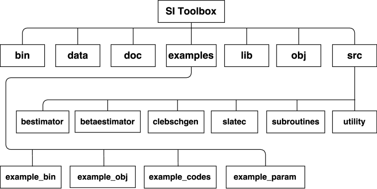
Figure 1: The directory structure for SIToolbox distribution.

3   SIToolbox directory structure

The directory structure of SI Toolbox is shown in Fig. 1. Here we broadly discuss the directory structure.

• SIToolbox/bin: It is a standard sub-directory that contains the executable (i.e., ready to run) programs. Initially this directory will be empty. After running the ./compile.sh command it will store the executable.

• SIToolbox/obj: It stores temporary object files while compiling the code. The object files can be removed once compilation is done.

• SIToolbox/lib: This subdirectory contains the SIToolbox library files. Initially it will be an empty directory. After running ./compile.sh it will store two library files namely libslatec.a and libsubroutines.a. Users, who like to write their own packages using the callable SIToolBox subroutines need to include these libraries while compiling their codes.

• SIToolbox/doc: This subdirectory contains the documentation of the SI Toolbox package and the related papers.

• SIToolbox/data: This subdirectory suppose to contain some non-isotropic maps and Clebsch Gordan coefficient files, bias function for the Doppler modulation and the $C_{l}$ corresponding to the bias function etc. These can be used for initial testing the proper compilation before running it on some real dataset. Presently no dataset is there in this directory due to file size restriction in github. The Clebsch Gordan coefficients can easily be generated using the clebschgen routine provided with this package.

• SIToolbox/source: This sub-directory contains the source codes. There are 6 sub-directories inside this folder, namely bestimator, betaestimator, clebschgen, utility, slatec, subroutines. The details of the first 4 are discussed in Sec. 5 and the last two are discussed in Sec. 6.

• SIToolbox/examples: Inside this directory there are few example codes which can help those who wants to develop their own packages.

4   SI Toolbox Installation Guideline

SI toolbox is written in Fortran 90. Therefore, you need some fortran compiler and openmp library for compiling the program . The package also uses HEALPix [6] and CFITSIO library.

Required packages

• HEALPix: HEALPix is a map projection software and it is extensively used for CMB data analysis. It can be downloaded from http://healpix.sourceforge.net/

  You need the library files libhealpix.a, libhpxgif.a.

• CFITSIO: CFITSIO is a library of C and Fortran subroutines for reading and writing data files in FITS (Flexible Image Transport System) data format. It can be downloaded from https://heasarc.gsfc.nasa.gov/fitsio/fitsio.html

  You need the library files libcfitsio.a.

• OpenMP: The parallelization is done with OpenMP. You need the files fopenmp and xopenmp for compiling SIToolBox.

All these packages should be available in your system before compiling SIToolBox.

For compiling the package, go to the SIToolBox folder. Open the compile.sh file in some text editor and set the path of your local F90 compiler, HEALPix, CFITSIO, OpenMP library files and HEALPix include files. It should look something as follows

# F90 Compiler
FC="/../intel/mpich-3.0.4/bin/mpif90"

#INCLUDE Path, LIB Path, FLAG Path
INCLUDE="-I/../Healpix_2.15a/include"
LIB="-L/../Healpix_2.15a/lib -L/../cfitsio -lhealpix -lhpxgif -lcfitsio"
FLAG="-fopenmp"
-------------

Give execute permission to the file compile.sh using the following command

chmod a+x compile.sh

Once compile.sh has the execute permission just run compile.sh using the command

./compile.sh

This will compile all the main codes. There are few example codes inside the folder /examples For compiling the example codes first give the execute permission to the compile.sh file inside /examples directory, change the F90 compiler, HEALPix, CFITSIO, OpenMP library path in compile.sh and then run the command ./compile.sh inside that folder. It will compile all the example codes.

5   Available standalone processes

5.1   betaestimator

This facility privides a means to generate the Monte Carlo chains for the Doppler $\beta$ parameter from a non-isotropic skymap assuming that the isotropy violation in the skymap is only due to the Doppler boost [1, 2]. However, this facility can also be used for the estimation of the Dipole modulation parameter, where the equations are similar to the Doppler boost.

Location inside SIToolbox directory
 

SIToolbox/src/betaestimator/

Details of the codes
  There are 4 FORTRAN programs inside the folder independent of each other (except the common subroutines they are calling). A brief detail of each of the program is given here so that users can customize the programs accordingly.

• betaestimator.f90 : It is the wrapper program for reading the input parameter file and calling the appropriate subroutine.

• beta_estimation_nonoise.f90 : It generates the Monte-Carlo chains for beta values when there is no noise in the map. In such cases, we don’t need to evaluate the $a_{lm}$s, as they are fixed. So the process is very fast. In single processor it takes just few minutes to finish the calculations.

• beta_estimation_isotropicnoise.f90 : It generates the Monte-Carlo chains when there is some isotropic noise in the map. In such cases we can calculate the noise variance inverse in the spherical harmonic space making it less time consuming than the anisotropic case.

• beta_estimation_anisotropicnoise.f90 : Generates the Monte-Carlo chains for beta parameter when noise in the sky is anisotropic or there is masking or both. In such case it is not possible to invert the noise matrix in the spherical harmonic space. So we need to go to the pixel space and invert the matrix pixel by pixel. This process is time consuming and runs about 3 times slower than beta_estimation_isotropicnoise.f90.

How to run
 

% betaestimator < betaestimator.in

Example parameter file
 

SIToolbox/examples/example_param/betaestimator.in

Here we briefly discuss the details of the variables in the parameter file.

Name	Example Value	Description
NOISE	no-noise	Type of Noise : (no-noise / isotropic / anisotropic)
MASK	yes	Do you want masking? (yes / no)
CLEBSCH_PATH	/home/sdas33/DATA/Final_beta_estimation/clebsch/clebs.dat	Precalculated Clebsch Gordan Coefficients ($C_{l1l2m1m2}^{LM}$) file.
CLEBSCH_Lmax	2	$L^{max}$ for the Clebsch Gordan file (for which the file has been generated).
CLEBSCH_l1max	1024	$l_{1}^{max}$ for the Clebsch Gordan file (for which the file has been generated).
SHAPE_FACTOR_PATH	/home/sdas33/DATA/SIToolBox/examples/fs.d	Shape factor file with the full path (shape factor must be written in Hazian-Souradeep format [7, 8, 4])
MASK_PATH	/home/sdas33/DATA/Data_SIToolBox/mask/wmapmask_E_con.d	Mask map file name along with full path. For no masking you can leave it blank.
CL_PATH	Planck2015TTlowP_totCls.dat	$C_{l}$ of the input map. In betaestimator we are not varying $C_{l}$. If you don’t have the best fit $C_{l}$, then you can calculate it using bestimator and then use it for betaestimator.
PIXEL_WINDOW_FUNCTION	pixel_window_n0512_t1.txt	HEALPix pixel window function for the given $N_{side}$.
NOISE_SD_PATH	/home/sdas33/DATA/SIToolBox/data/Nmap.d	Anisotropic Noise standard deviation map file name along with full path. For isotropic noise you can leave it blank.
NOISE_SD	30.0	Noise standard deviation in pixel space if NOISE=isotropic. Otherwise you can keep it blank or set any random value. Unit is same as the unit used in the map.
MAP_PATH	/home/sdas33/DATA/SIToolBox/data/Tmap.d	Enter the input map path. Map should be in ASCII format and ordering is RING. (For fits files you need to convert it to ASCII format using fits2d command)
MAP_NSIDE	512	Nside of the map
CHAIN_PATH	/home/sdas33/DATA/SIToolBox/examples/Bestimator_Chain/	Location of the folder where the chain will be stored. One run can generate only one chain. To generate multiple chains you can submit the code multiple times but the Chain folder should be different for each of the submission. Otherwise it will mix the values.
CHAIN_Lmax	2	$L^{max}$ for the BipoSH chains.
CHAIN_l1max	1024	$l_{1}^{max}$ for the BipoSH chains.
SAMPLE_NUMBER	5000	Number of sample points for Monte-Carlo chain of the $\beta$ parameter.

5.2   bestimator

This facility provides a means to generate the Monte-Carlo chains for BipoSH coefficients from a non-SI skymap [1, 2]. We do not provide any facility to calculate the BipoSH chains for no noise case because there are trivial analytic solutions for that case. However, someone can easily simulate such cases by setting the noise variance to a negligibly small value. The values in the output file are written in Hazian-Souradeep format.

Location inside SIToolbox directory
 

SIToolbox/src/bestimator/

Details of the codes
  There are three Fortran programs inside the directory independent of the programs in other directory. So users can easily modify the programs according to their own requirements. Brief details of the programs are as follows.

• bestimator.f90 : Its the wrapper for reading the input file and running the appropriate subroutine.

• BipoSH_ALMll_isotropic_Noise : Generates the BipoSH Chains from a map with isotropic noise. For isotropic noise, $N_{lml^{\prime}m^{\prime}}$ being a diagonal matrix, is invertible in the spherical harmonic space making the process less time consuming.

• BipoSH_anisotropic_noise : Generates the BipoSH chains when noise field is anisotropic. Here, $N_{lml^{\prime}m^{\prime}}$ is not a diagonal matrix and hence the inversion is not possible in spherical harmonic space. So we go to the pixel space and invert the matrix pixel by pixel. This process is time consuming and runs about 3 times slower then the isotropic noise case.

How to run
 

% bestimator < bestimator.in

Input parameter file
 

SIToolbox/examples/example_param/bestimator.in

Here we briefly discuss the details of the variables in the parameter file.

Name	Example Value	Description
NOISE	isotropic	Type of Noise: (isotropic / anisotropic)
MASK	yes	Do you want masking? (yes / no)
CLEBSCH_PATH	/home/sdas33/DATA/Final_beta_estimation/clebsch/clebs.dat	Precalculated Clebsch Gordan Coefficients $C_{l1l2m1m2}^{LM}$ file with full path.
CLEBSCH_Lmax	2	$L^{max}$ for the Clebsch Gordan file.
CLEBSCH_l1max	1024	$l_{1}^{max}$ for the Clebsch Gordan file.
NOISE_SD_PATH	/home/sdas33/DATA/SIToolBox/data/Nmap.d	Filename with the full path of the anisotropic noise standard deviation file if NOISE=anisotropic. Otherwise leave it blank or put some arbitrary value.
NOISE_SD	30.0	Noise standard deviation in pixel space, if NOISE=isotropic
MASK_PATH	/home/sdas33/DATA/Data_SIToolBox/mask/wmapmask_E_con.d	Mask map file name along with full path. For no masking you can leave it blank.
MAP_PATH	/home/sdas33/DATA/SIToolBox/data/Tmap.d	Map file name with full path. Map should be in ASCII format and ordering is RING.
PIXEL_WINDOW_FUNCTION	pixel_window_n0512_t1.txt	HEALPix pixel window function for the given $N_{side}$.
MAP_NSIDE	512	HEALPix Nside of the map.
CHAIN_PATH	/home/sdas33/DATA/SIToolBox/examples/Bestimator_Chain/anisotropic	Location of the folder where the chain will be stored. One run can generate only one chain. For multiple runs you must specify different chain folders.
CHAIN_Lmax	2	$L^{max}$ for the BipoSH chains.
CHAIN_l1max	1024	$l_{1}^{max}$ for the BipoSH chains.
SAMPLE_NUMBER	5000	Number of sample points in the BipoSH chains. You can also run multiple small chains separately and then merge the files.

Output chain files
  We follow the following conversion for the output chain file names

A(R/I)_(LM)_ll(d).d

where, ‘R’ or ‘I’ stands for the real and the imaginary parts of the coefficients. L and M are the L and M values of $A_{ll-d}^{LM}$ and d is the difference between $l_{1}$and $l_{2}$. So the file AR_10_ll1.d stores real part of $A_{ll-1}^{10}$.

5.3   map2fits, fits2d, nest2ring, ring2nest, rotateCoor

These are the utility facilities and provide handy means for pre/post processing of the data. These stand alone facilities are based on different HEALPix subroutines.

The first two facilities, namely map2fits and fits2d provide a means to convert a map from ASCII to fits and vice-versa. These conversions will preserve the ordering (NESTED or RING) of the input map. Except these two facilities all the other standalone facilities provided in SIToolbox run on the ASCII files.

The next two facilities, namely nest2ring and ring2nest provide a means to change the ordering of the input map, from RING ordering to NESTED ordering or vice-versa. All the estimator codes in SIToolbox run on the RING ordering. So in many cases, converting the map between two ordering is important.

The last facility, i.e. rotateCoor will convert the map from one coordinate system to another coordinate system. The input and output coordinate systems are Galactic, Ecliptic, Celestial and Equatorial.

Location inside SIToolbox directory
 

SIToolkit/src/utility/map2fits.f90	SIToolkit/src/utility/fits2d.f90
SIToolbox/src/utility/nest2ring.f90	SIToolbox/src/utility/ring2nest.f90
SIToolbox/src/utility/rotateCoor.f90

How to run
  You can run these facilities interactively using Linus shell. Here we show an interactive run of fits2d facility. Runs are in general self-explanatory.

% fits2d
  Enter Nside for the map
  512
  Enter the input map
  map.fits
  Successful conversion
  Enter the output file name
  map.d

Input parameters
 

Name	Description
Nside	HEALPix Nside for the Input and Output map
Input Map	File name with full path of the Input map. Except fits2d all the other inputs must be in ASCII format.
Output Map	Output file name with full path. Except map2fits the output file should be in ASCII format everywhere else.
Ordering	For map2fits you need to specify the ordering of the file for writing in the header. Choices are ( 1 / 2 ), where 1.RING and 2.NESTED. Default ordering is RING ordering.
Input/Output Coordinate	For rotateCoor you have to specify the input/output coordinate system of the file. Options are G. Galactic, E. Ecliptic, C. Celestial and E. Equatorial.

5.4   clebschgen

This facility privides a means to generate the Clebsch-Gordan coefficients ($C_{l_{1}m_{1}l_{2}m_{2}}^{LM}$) file for BipoSH calculation, bestimator and betaestimator. This facility uses the slatec library for calculating the Clebsch-Gordan coefficients. It calculates all the nonzero Clebsch Gordan coefficients, given a maximum value of $L^{max}$ and $l_{1}^{max}$ and store them in a file.

Note that, as we are writing all the values of Clebsch-Gordan coefficients in a file, it is necessary to read the full file before calculating a particular Clebsch Gordan coefficient. However, if you are interested in a particular Clebsch Gordan coefficient or a couple of them then you can directly call the clebsch stand alone function.

Location inside SIToolbox directory
 

SIToolbox/src/clebschgen/clebschgen.f90

How to run
  Here we present a simple run of the program clebschgen. Interactive run is self explanatory. We just need to provide $L^{max}$ and $l_{1}^{max}$ for the Clebsch-Gordan coefficients. The output file name will be chosen by the program.

% clebschgen
  Program : clebschgen
  It will calculate Clebsch Gordan coefficients C^{L M}_{l1 m1 l2 m2}
  Please input L_max and l1_max
  2 1024
  Output Clebsch filename : Clebs_Lmax_2_lmax_01024.dat

Input parameters
 

Name	Description
L_max	Maximum value of $L$ in $C_{l_{1}m_{1}l_{2}m_{2}}^{LM}$
l1_max	Maximum value of $l_{1}$ in $C_{l_{1}m_{1}l_{2}m_{2}}^{LM}$

Output File
  Clebs_Lmax_*_lmax_*.dat : It stores the $C_{l_{1}m_{1}l_{2}m_{2}}^{LM}$ values up to $L^{max}$ and $l_{1}^{max}$. The file has two columns. The first column is the one dimensional index of the of the Clebsh Gordan coefficient and the second column is the Clebsh-Gordan coefficient. The one dimensional index of $C_{l_{1}m_{1}l_{2}m_{2}}^{LM}$ in the file is given by ClbIndex that can be obtained by calling the subroutine

Clebsch2OneD(L,M,l1,l2,m1,lmax,ClbIndex).

We can open the file in FORTRAN by calling

open(1,file=’****’, action=’read’,status=OLD)

and read the file in an array by calling

      read(1,*)recno,cleb
      Clebs(recno)=cleb

We can get the ClbIndex-th value by Clebs(ClbIndex). Note that, the file only stores the values for $l_{1}<l_{2}$. For $l_{1}>l_{2}$ We need to use the properties of the Clebsch-Gordan coefficients to calculate it from $l_{1}<l_{2}$ values.

Example code for reading output file
 

SIToolBox/examples/example_codes/test_readClebs.f90

6   Available callable subroutines

6.1   lm2n, n2lm

The first subroutine, i.e. lm2n( ) is useful for storing two dimensional $a_{lm}$ into a single dimensional array $q_{n}$. This is useful because if we allocate $a_{lm}$ as

allocate(alm(0:lmax, 0:lmax))

then half of the allocated spaces will not be used. However, if we write it as a single dimensional array then it will help while passing the variable into different functions or different MPI processors. Also, for calling the function CalcBipoSH we need one dimensional array of $a_{lm}$ that can be generated using lm2n( ) subroutine.

We can convert the one dimensional array back to two dimensional $a_{lm}$ array using n2lm( ).

Format
 

call lm2n(l,m,n)           OR           call n2lm(n,l,m)

Arguments
 

Name	Kind	In/Out	Description
l	INT	IN / OUT	$l$ value of $a_{lm}$
m	INT	IN / OUT	$\texttt{abs}(\texttt{m})$ value of $a_{lm}$. This variable can only take values from $0$ to $l$.
n	INT	OUT / IN	Array index in the single dimensional array.

Example
 

integer :: n,l,m l=20 m=14 ! m must be positive call lm2n(l,m,n) write(*,*) n end program

OR

integer :: n,l,m n=224 call n2lm(n,l,m) write(*,*) l,m end program

Location of Example code
 

SIToolbox/examples/example_codes/test_lm2n.f90

SIToolbox/examples/example_codes/test_n2lm.f90

6.2   Clebsch2OneD

Saving the Clebsch-Gordan coefficients in one dimensional format is useful instead of 6 dimensional matrices because most of the values of the Clebsch-Gordan coefficients are zero. So instead of saving it in 6 dimensional matrix if we store it in a one dimensional matrix then it will save a lots of memory. It is also helpful while storing the array in a direct access file or reading it from there.

Format
 

call Clebsch2OneD(L,M,l1,l2,m1,lmax,ClbIndex)

Arguments
 

Name	Kind	In/Out	Description
L, M	INT	IN	Array index of one dimensional representation of $C^{LM}_{l_{1}m_{1}l_{2}m_{2}}$.
l1, l2	INT	IN	$l_{1}$ and $l_{2}$ index of $C^{LM}_{l_{1}m_{1}l_{2}m_{2}}$.
m1	INT	IN	$m_{1}$ index of $C^{LM}_{l_{1}m_{1}l_{2}m_{2}}$
lmax	INT	IN	Maximum value that $l_{1}$ can take
ClbIndex	INT	OUT	Output one dimensional index of the Clebsch-Gordan coefficient.

Example
 

integer :: L,M,l1,l2,m1,lmax
integer :: ClbIndex

L=2 M=1
l1 = 1000  l2 = 1001 m1 = 578
lmax = 1024

call Clebsch2OneD(L,M,l1,l2,m1,lmax,ClbIndex)
write(*,*) ClbIndex
end program

Location of Example code
 

SIToolBox/examples/example_codes/test_Clebsch2OneD.f90

6.3   CalcBipoSH

This subroutine calculates the BipoSH coefficients from some input map. The output BipoSH coefficients from this function will be in the Hazian Souradeep format, which can be converted to the WMAP-7 format by multiplying with $\frac{\sqrt{2L+1}}{\sqrt{2l+1}\sqrt{2l^{\prime}+1}}\frac{1}{C_{l0l^{\prime}0}^{L0}}$ [1].

Format
 

call CalcBipoSH(Qr,Qi,LMAX,llmax,ALMll,ALMlli,Clebs)

Arguments
 

Name	Kind	In/Out	Description
llmax	INT	IN	Maximum value that $l_{1}$ can take
LMAX	INT	IN	Maximum value of $L$ in $A_{l_{1}l_{2}}^{LM}$.
Qr(0:dim-1), Qi(0:dim-1)	DP	IN	Real and imaginary part of $a_{lm}$s when written in a single dimensional array.
ALMllr(0:LMAX,0:LMAX, 0:llMAX,-LMAX:LMAX), ALMlli(0:LMAX,0:LMAX, 0:llMAX,-LMAX:LMAX)	DP	OUT	Real and Imaginary parts of the output BipoSH coefficients
Clebs(:)	DP	IN	Pre-calculated Clebsch-Gordan coefficients as a single dimensional array.

Example
 

use healpix_types
use alm_tools
use pix_tools
use omp_lib

integer,parameter :: LMAX = 2
integer,parameter :: llMAX = 1024
integer :: nside = 512
integer :: i,j,k
real(sp), allocatable, dimension(:,:) :: Map
real(dp),allocatable,dimension(:) :: Clebs
real(dp), allocatable, dimension(:) :: Qr,Qi
real(dp) :: ALMllr(0:LMAX,0:LMAX,0:llMAX,-LMAX:LMAX)
real(dp) :: ALMlli(0:LMAX,0:LMAX,0:llMAX,-LMAX:LMAX)
real(dp) :: Clebs(0:35000000)
complex(spc), allocatable, dimension(:,:,:) :: alm

...........

allocate(Qr(0:(llmax+1)*(llmax+2)/2-1))
allocate(Qi(0:(llmax+1)*(llmax+2)/2-1))
allocate(Map(0:12*nside*nside-1,1:3))
allocate(alm(1:3, 0:llmax, 0:llmax))

...........

!! READ THE MAP

...........

dw8 = 1.0_dp
z = (-1.d0,1.d0)
call map2alm(nside, llmax, llmax, map, alm, z, dw8)

...........

!! READ THE CLEBSCH GORDAN COEFFICIENTS

...........

k = 0
do i = 0,llmax
do j = 0,i
Qr(k)=real(alm(1,i,j))
Qi(k)=aimag(alm(1,i,j))
k = k+1
end do
end do

call CalcBipoSH(Qr,Qi,LMAX,llmax,ALMllr,ALMlli,Clebs)

.........

end program

Location of Example code
 

SIToolBox/examples/example_codes/test_CalcBipoSH.f90

6.4   clebsch, drc3jj, drc3jm

These are the slatech subroutines and these can be used for calculating the Wigner 3j symbols and the Clebsch-Gordan coefficients.

Format
 

CALL DRC3JM(l, l1, l2, -m, m1min, m1max, THRCOF, NDIM, IER)

CALL DRC3JJ(l1, l2, m1, m2, l1min, l1max, THRCOF, NDIM, IER)

CALL clebsch(l, l1, l2, m, m1min, m1max, cleb, NDIM, IER)

Arguments
 

Name	Kind	In/Out	Description
l, l1, l2	DP	IN	$l$, $l_{1}$, $l_{2}$ values for Wigner 3j symbol or Clebsch–Gordan coefficients
m, m1, m2	DP	IN	$m$, $m_{1}$, $m_{2}$ values for Wigner 3j symbol or Clebsch–Gordan coefficients
NDIM	INT	IN	Allocated dimension of the output matrix. This should be more than or equal to the dimension of the output array of Wigner 3j symbol or Clebsch–Gordan coefficients. For example, suppose you are calling DRC3JM for values $l=1$,$l_{1}=100$, $l_{2}=100$ and $m=1$. So output array gives Wigner 3j for different values of $m_{1}$. Now for this set of parameters $m_{1}$ can take $201$ different values. So the dimension of the output array will be $201$. So NDIM has to be more than or equal to 201.
m1min , m1max , l1min , l1max	DP	OUT	minimum and maximum values of $m_{1}$ or $l_{1}$ that we can have for the particular set of parameters.
THRCOF(1:NDIM), cleb(1:NDIM)	DP	OUT	The output array of Wigner 3j symbol or Clebsch–Gordan coefficients.
IER	INT	OUT	Error flags : 1. IER=0 No errors. 2. IER=1 Either L2.LT.ABS(M2) or L3.LT.ABS(M3). 3. IER=2 Either L2+ABS(M2) or L3+ABS(M3) non-integer. 4. IER=3 L1MAX-L1MIN not an integer. 5. IER=4 L1MAX less than L1MIN. 6. IER=5 NDIM less than L1MAX-L1MIN+1.

Example
 

integer ier,i,tot
parameter (NDIM=500)
real*8 l,l1,l2,m,m1,m2,m1min,m1max,l1min,l1max
real*8 THRCOF(NDIM),cleb(NDIM)

l=1 l1=101 l2=100 m=1
CALL DRC3JM(l, l1, l2, -m, m1min, m1max, THRCOF, NDIM, IER)
tot = int(m1max-m1min)+1
write(*,*)THRCOF(1:tot)

l1=101 l2=100 m1=50 m2=100
CALL DRC3JJ(l1, l2, m1, m2, l1min, l1max, THRCOF, NDIM, IER)
tot = int(l1max-l1min)+1
write(*,*)THRCOF(1:tot)

l=1 l1=101 l2=100 m=1
CALL clebsch(l, l1, l2, m, m1min, m1max, cleb, NDIM, IER)
tot = int(m1max-m1min)+1
write(*,*)cleb(1:tot)

return end

Location of Example code
 

SIToolBox/examples/example_codes/test_slatec.f90

References

- [1] S. Das, B. D. Wandelt, and T. Souradeep, Bayesian inference on the sphere beyond statistical isotropy, JCAP 1510 (2015), no. 10 050, [arXiv:1509.0713].
- [2] S. Das, Sitoolbox : A package for bayesian estimation of statistical isotropy violation in the cmb sky, arXiv:1810.0947.
- [3] N. Pant, S. Das, A. Rotti, S. Mitra, and T. Souradeep, Estimating statistical isotropy violation in CMB due to non-circular beam and complex scan in minutes, JCAP 1603 (2016), no. 03 035, [arXiv:1511.0367].
- [4] S. Das, S. Mitra, A. Rotti, N. Pant, and T. Souradeep, Statistical isotropy violation in WMAP CMB maps resulting from non-circular beams, Astron. Astrophys. 591 (2016) A97, [arXiv:1401.7757].
- [5] S. Mukherjee, A. De, and T. Souradeep, Statistical isotropy violation of CMB Polarization sky due to Lorentz boost, Phys. Rev. D89 (2014), no. 8 083005, [arXiv:1309.3800].
- [6] K. M. Gorski, E. Hivon, A. J. Banday, B. D. Wandelt, F. K. Hansen, M. Reinecke, and M. Bartelman, Healpix – a framework for high resolution discretization, and fast analysis of data distributed on the sphere, astro-ph/0409513v1.
- [7] A. Hajian and T. Souradeep, Measuring statistical isotropy of the CMB anisotropy, Astrophys. J. 597 (2003) L5–L8, [astro-ph/0308001].
- [8] N. Joshi, S. Das, A. Rotti, S. Mitra, and T. Souradeep, Revealing Non-circular beam effect in WMAP-7 CMB maps with BipoSH measures of Statistical Isotropy, arXiv:1210.7318.