Propulsion and Mixing Generated by the Digitized Gait of Caenorhabditis elegans

Abstract

Nematodes have evolved to swim in highly viscous environments. Artificial mechanisms that mimic the locomotory functions of nematodes can be efficient viscous pumps. We experimentally simulate the motion of the head segment of Caenorhabditis elegans by introducing a reciprocating and rocking blade. We show that the bio-inspired blade’s motion not only induces a flow structure similar to that of the worm, but also mixes the surrounding fluid by generating a circulatory flow. When confined between two parallel walls, the blade causes a steady Poiseuille flow through closed circuits. The pumping efficiency is comparable with the swimming efficiency of the worm. If implanted in a sealed chamber and actuated remotely, the blade can provide pumping and mixing functions for microprocessors cooled by polymeric flows and microfluidic devices.

I Introduction

Emerging technologies in microprocessor cooling, polymeric flows, and in the pharmaceutical and chemical industries require the resolution of numerous theoretical and practical challenges posed by pumping and mixing in low Reynolds number conditions. In practice, pumping and mixing are regarded as two different functions, and engineered systems usually have separate units to perform these tasks. Widely used syringe, peristaltic, and piezo pumps do not mix flowing liquids, and few mixing protocols are known. In microchannels where the Reynolds number is low, as the liquid is circulated by an external pump, passive mixing is achieved by special carvings on the channel walls stroock2002chaotic . The well-known active mixing protocol is a rod moving in a figure-eight trajectory gouillart2007walls , but this protocol has not been tested for pumping. On the other hand, in natural systems, we know little about the interconnection between the pumping and possible mixing of blood in small-scale living beings. For instance, early cardiac function in embryonic vertebrates occurs in low Reynolds number conditions, and the propagation of elastic waves seems to pump the blood forouhar2006embryonic . We do not know if such traveling waves, preferred by nature, can also mix the blood. The combination of the pumping and mixing functions in a single artificial mechanism is an unsolved problem, which we tackle in this work.

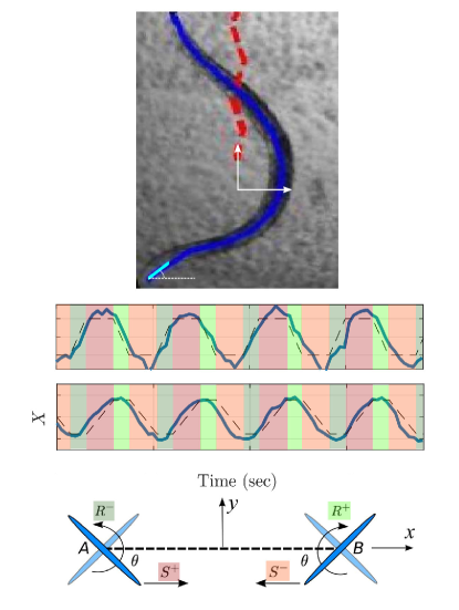
Figure 1: Digitizing the head movement of C. elegans. (a) The shape of C. elegans in its undulatory gait (cf. sznitman2010material ; gray1964locomotion ; stephens2008dimensionality ). The C. elegans is shown in blue, the head is shown in cyan, and the red dashed line represents the recorded motion of its center of mass. (b) The angle and position of the head of C. elegans in solid blue lines. The head pushes the surrounding fluid, switches its orientation after a transitional phase, then pushes the fluid in the opposite direction. The dashed lines represent the digitized approximation of the motion of head. Snapshots are taken from videos of the behavior of C. elegans in Ref. sznitman2010material . (c) A schematic demonstration of the reciprocating and rocking motion of a blade that simulates the head of C. elegans. Each stage of motion is color coded to match with (b).

A naturally inspired way of propulsion and mixing in low Reynolds number conditions is to replicate the locomotory function of microorganisms dreyfus2005microscopic ; shields2010biomimetic ; jalali2015microswimmer ; mirzakhanloo2018hydrodynamic ; mirzakhanloo2018flow , especially ones that can swim in various environmental conditions by adapting their gaits. Experimental studies show that when C. elegans swims in water, the Reynolds number $Re$ exceeds 0.2 backholm2015effects , and the worm’s head undergoes a flapping oscillation with one degree of freedom and almost no traveling wave along its body (see Fig. 10A in Ref. fang2010biomechanical ). Increasing the viscosity of the surrounding fluid dramatically changes the gait: a quasi-periodic wave travels from the head to tail, the undulatory wavelength drops, and the head segment exhibits a combination of flapping and translational motions fang2010biomechanical ; sznitman2010material . We have analyzed videos of C. elegans movements and extracted a sequence of snapshots of its body configuration over a period of undulatory gait (Fig. 1A). It is seen that the head tends to push the surrounding fluid before it flips and there exists a phase difference between its translational and rotational motion (Fig. 1B). We “digitize” the movement of the head by approximating it with a linear translation followed by a rotational motion with $\pi/2$ phase difference, and model the head by a thin rigid blade (Fig. 1C). The phase difference between translational and rotational motion breaks the time symmetry of motion, and plays an essential role in creating a net fluid flow at low Reynolds. It is to be noted that C. elegans gains a total thrust from its tail, body, and head segments and here we only digitize the head movement as a bio-inspired motion generating propulsion and mixing.

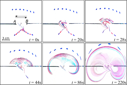
Figure 2: Propulsion and mixing by a reciprocating and rocking blade. The blade’s shaft moves along the black slit. Two rows of dyes have been injected into the surface of the fluid. The lower set is composed of a sequence of blue and red dyes, which have had an initial distance of $4.4$ cm from the blade’s path. The upper blue dyes had an initial distance of $5$ cm from the slit. Snapshots have been taken when $\dot{x}>0$ and the blade is half way from the end points of its path. The stroke length is $AB=4.5$ cm. The resolution of camera is $1920\times 1080$ pixels. We have maximized the exposure with linear Gamma correction of the pictures to eliminate the color of the background fluid.

Our experimental apparatus consists of a blade with two degrees of freedom that moves in a viscous fluid. Figure 1C shows the edge view of the blade, which undergoes a rectilinear motion in the $x^{+}$ direction ($S^{+}$) with the constant angle of attack $\theta$, then stops at point $B$ and rotates by $\pi-2\theta$ in the clockwise direction ($R^{+}$). It then moves in the $x^{-}$ direction ($S^{-}$) until it stops at point $A$, makes a counter-clockwise turn of $\pi-2\theta$ ($R^{-}$), and repeats the sequence $S^{+}\rightarrow R^{+}\rightarrow S^{-}\rightarrow R^{-}$. During the translational and rotational phases, the linear and angular velocities are set to constant values $v_{0}$ and $\omega_{0}$. In accordance with the gait of C. elegans, we set $\theta=45^{\circ}$. Sufficiently far from the blade where geometric effects diminish, the velocity field becomes a Stokeslet $\sim v_{0}r^{-1}$ during $S^{\pm}$ stroke phases, and the rotations $R^{\pm}$ generate rotlets scaled as $\sim\omega_{0}r^{-2}$ with $r$ being the radial distance from the blade’s center.

II Experimental Results

We use a gantry $x$-$y$ table with a stepper motor M1 that controls the horizontal $x$-coordinate of a second servo motor M2. We couple motor M2 to a vertical shaft (in the $z$ direction) that holds a circular, aluminum blade at its other end. The blade rotates around the $z$-axis, and its angle of attack $\theta$ is controlled by motor M2. The diameter and thickness of the blade are $D=30\,{\rm mm}$ and $w=0.8\,{\rm mm}$, respectively. The fluid is corn syrup with density $\rho=1.34\,{\rm g/cm^{3}}$ and kinematic viscosity $\nu=41\,{\rm cm^{2}/s}$. In order to study the free surface flow, the blade is half submerged in the liquid, and we inject color dyes at the surface. We use red and blue food colors as tracer dyes and dissolve them in corn syrup before injecting into the surface. This minimizes the effect of diffusion and possible interactions between dyes cira2015vapour . We introduce two rows of dyes on both sides of the line segment $AB$. A two-color sequence is used in the lower row to study and visualize the mixing function of the blade (Fig. 10).

We actuate the blade by setting $v_{0}=2.5$ cm/s and $\omega_{0}=5\pi/2$ rad/s. These yield a low-Reynolds-number condition—with $Re\approx 0.12$—relevant to the swimming and crawling of C. elegans. Each motion cycle has a period of $T=4\,{\rm s}$. Figure 10 and Supplementary Material video 1 supp-videos display how initially round dyes evolve as the time elapses. They are first pumped toward the blade, then stretched and folded as they cross the $x$-axis. After passing through the blade, they form a wavelike structure that propagates in the $y^{+}$ direction and is similar to the trace that the head of a wild type C. elegans leaves behind sznitman2010material . The wavelength of the streaming field decreases as tracers depart from the blade. This is due to the decline in the velocity magnitude of the Stokeslet field. Furthermore, the rocking motion of blade creates circulatory streams on the two sides of the blade as it translates. To show this effect, we have conducted an experiment by setting $\omega_{0}=0$ and traced the trajectories of mm-size tracer particles using image processing techniques. Supplementary Material video 2 supp-videos shows how circulatory streams form on the two sides of the blade. The observed flow structure is reminiscent of recirculatory streams attached to each segment of the body of C. elegans gray1964locomotion ; shen2011undulatory , including its head.

The waving stream is then pulled sideways by rotlet fields generated at points $A$ and $B$, folded as a kidney-shaped bundle, and sucked by the blade from the lower side. The emerging circulatory flow diverts fluid elements from the entire domain toward the line segment along which the blade reciprocates. This is evident from the trajectories that the stretched and folded blue dyes, initially located on the upper side of the blade, follow until they reach the blade. The mixing function of the mechanism is deduced from the disappearance of initially blue and red colors and the emergence of a mixed color within the kidney-shaped structure at $t=220\,{\rm s}$ and afterwards. Mixing is characterized by the recurrence time of fluid elements to the line segment $AB$. The larger the initial radial distance from the blade, longer the circulation of deformed elements and their revisit of the blade. Repeated stretching and folding of fluid elements by $S^{\pm}$ Stokeslets, $R^{\pm}$ rotlets and the blade, are analogous to the horseshoe map and suggest chaotic mixing which we later numerically quantify.

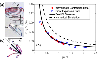
Figure 3: Forward pumping by the blade. (a) The fluid stream and its waveform with the decreasing wavelength $\lambda$. The temporal distances between successive peaks are identical. The front curve $F$ is expanding. The snapshot has been taken at $t=60$s. (b) The average velocity in the $y$ direction when the blade is passing through $x=0$. (c) The flow structure in the vicinity of the blade at $t=17$s. The region between the two dashed lines is impenetrable due to adhesion and surface tension effects.

The envelope of the kidney-shaped structure is expanding. This is an indicator of the pumping function, which we quantify by measuring the average streaming velocity $\langle v_{y}\rangle$ along the $y$-axis. It is to be noted that in the rocking and rotating motion, the fluid is pushed in the normal direction to the blade’s plane, and the averaged motion of fluid determines the net pumping effect and its direction. We measure the expansion rate through two methods: the contraction rate of the wavelength $\lambda$, and the expansion rate of the front $F$ (Fig. 11A). In the first technique, we analyze the snapshot at $t=60\,{\rm s}$ well before the mixing process dissolves the sharp features of the developing streamlines, and in the second method, we follow the front curve $F$ in the strobe images taken with increments of $T=4\,{\rm s}$. Figure 11B illustrates the experimental values of $\langle v_{y}\rangle$ versus $y$. Our mean experimental error level is about $4\%$, which is mainly due to the perspective image distortions of the camera.

III Numerical Results

We further test the setup using Finite Element Methods. We simplify the problem to a two dimensional flow where the fluid velocity $\mathbf{u}=(u,v)$ and pressure $p$ satisfy

$$\Delta\mathbf{u}+\nabla p=0,$$

$$\nabla\cdot\mathbf{u}=0.$$

Each stage of blade’s motion (i.e., $S^{+},R^{+},S^{-},R^{-}$) is divided into $N$ snapshots and velocity field is obtained using finite element methods for each of the snapshots with proper boundary conditions describing the blade’s movement. The number $N$ is resolved until the numerical result converges (here $N=100$). Open source Finite Element Library FreeFEM++ hecht2012new is used to solve for the weak form of the equation. The variables are non-dimensionalized with $L=2$cm, $\mathscr{T}=1$s. The numerical domain is set to $[0,9.5]\times[0,29]$ to match the experimental setup. The numerical simulation borders are seeded using nodes spaced by $\delta x=0.2$, and $\delta x=0.005$ respectively; and the element mesh is then created using the FreeFEM++ mesh generator.

When the blade is at $x=0$, analytical calculations jalali2015microswimmer ; jalali2014versatile give $v_{y}/v_{0}=\Delta C\sin(2\theta)/[8\pi(y/D)]$ where $\Delta C$ is the difference between the coefficients of drag forces against the broad side and edge-wise motions of the blade. In the limit of a fully submerged, razor-thin disk ($w\rightarrow 0$) one finds $\Delta C=8/3$ happel2012low . Fitting an analytical function $\sim(y/D)^{-1}$ to experimental data, gives $\Delta C\approx 0.74$ (best-fit Stokeslet curve in Fig. 11B). Alongside the analytical calculation, we computed the front curve speed in our numerical simulation and found that it follows a $(y/D)^{-1}$ trend close to the experiment’s result (numerical simulation curve in Fig. 11B). To understand the origin of the observed difference between experimental results and analytical/numerical results, we have produced a close-up view of the flow field around the blade at $t=17$s and displayed it in Fig. 11C. Inspection of Fig. 11C shows that the flow separates from the leading edge of the blade and an impenetrable layer develops between two dashed lines. The thickness of the impenetrable layer depends on adhesion and surface tension effects ren2009adhesion . The blade and its associated impenetrable layer behave like a moving wedge. Therefore, the effective drag against edge-wise motion increases significantly and reduces the front speed: instead of a simple skin drag on the two faces of the disk, the edge-wise motion now experiences an extra form drag. Less adhesive surfaces can boost the pumping efficiency. Since the flow is at low Reynolds ($Re\ll 1$), it is apparent that increasing blade’s velocity would effectively increase the pumping velocity. On the other hand, the net effect of blade’s angle is less obvious; therefore we study the effect of blade angle in our digitized motion (see Fig. 4). The front speed first increases with the increase in blade’s angle until a maximum velocity profile is reached at $\theta=\pi/4$. After this optimal value, the velocity profile decreases significantly with the increase in blade’s angle. Note that at $\theta=0$ the rotational motion is present and contributes to pumping and mixing; however, at $\theta=\pi/2$ the rotational motion vanishes and the net motion becomes a time reversal translation which is unable to generate any pumping at low Reynolds. We further analyze a simultaneous sinusoidal rocking and rotational motion with $X=(l_{s}/2)\sin(2\pi t/T+\pi/2)$, $\theta=\pi/2-\pi/4\sin(2\pi t/T)$, where $l_{s}$ is the stroke length, and $T$ is the period of motion. As shown in Fig. 4, this simultaneous sinusoidal rocking and rotational motion creates a much higher wave front speed; however, because of experimental setup complexity is not studied here.

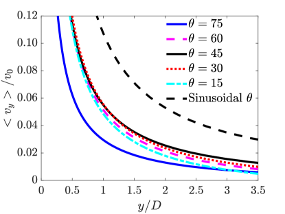
Figure 4: Numerical simulation results for the average velocity of the wave front in the y direction when the blade is passing through x = 0 for different values of the disk angle i.e. $\theta$. The maximum velocity profile in the digitized motion is obtained at $\theta=45$. A continuous sinusoidal rocking and rotational motion (dashed black line) has higher average velocity profile than the digitized versions of the motion.

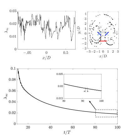
Figure 5: (a) The profile of $\lambda_{\infty}(\mathscr{L},100T)$ along the line segment $\mathscr{L}$, (b) The state of the line element represented by 200 tracer particles at $t=0$ (red dots) and $t=100T$ (black dots). The line segment is at the location of the lower set of dye in Fig. 10. The positions of the disks are shown in dark and light blue. (c) Time evolution of the maximum eigen-value over time for the mid-point $x=0$ in line segment $\mathscr{L}$. The time period of motion is $T$ and the inset figure shows a close up of the box shown. The time evolution of maximum eigen-value is a continuous curve with kicks that correspond to $R^{+}$ and $R^{-}$ segments of motion.

We utilize the finite time Lyapunov exponent to quantify the mixing process lapeyre2002characterization . We calculate finite time largest Lyapunov exponent $\lambda_{\infty}$ along a line segment corresponding to the red dye shown in Fig. 10 i.e $\mathscr{L}=\{(x,y)|-l_{s}/2\leq x\leq l_{s}/2,y/D=-1.45\}$ where $l_{s}$ is the length of stroke. A positive Lyapunov exponent, $\lambda_{\infty}>0$, implies chaos and therefore an exponential divergence of neighboring traces lying on $\mathscr{L}$. To compute the Lyapunov exponent for a particle initially at $X_{0}$, we integrate

$$\frac{\text{d}}{\text{d}t}M(t)=\mathbf{J}(\mathbf{X}(t),t)^{\top}M(t),$$

$$\quad\mathbf{J}=\nabla\mathbf{u},\quad M(0)=\mathbb{I},$$

where $M$ is called resolvent matrix. The finite time Lyapunov exponent $\lambda_{\infty}$ is then obtained as the logarithm of maximum eigenvalue of $(M^{\top}M)^{1/2t}$. Figure 5 shows the variation of $\lambda_{\infty}(\mathscr{L},t=100T)$. The state of 200 particles along $\mathscr{L}$ after $t=100T$ is shown in Fig. 5B. The time evolution of the maximum eigen-value for a sample point, the mid-point particle with $x=0$, is shown in Fig. 5C. The time evolution of maximum eigenvalue is a continuous line with kicks that corresponds to the $R^{+}$ and $R^{-}$ section of motion. We would like to point out that the Finite Element Simulation is a two dimensional low Reynolds approximation of the flow around the blade and it does not account for the free surface in the experimental setup. The free surface introduces surface tension at the blade’s point of contact which further reduces the pumping efficiency. Lastly, to show that the observed flow structure is reminiscent of recirculatory streams attached to each segment of the body of C. elegans gray1964locomotion ; shen2011undulatory , the numerically obtained circulatory motion of flow-field as the blade passes through $x=0$ is shown in Fig. 6.

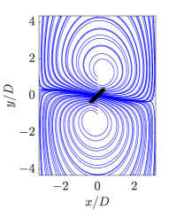
Figure 6: Flow-field streamlines computed from instantaneous velocity field in the vicinity of the blade (shown with black lines) when the blade is passing through $x=0$. The motion corresponds to rectilinear $S^{+}$ motion. Due to symmetry, streamlines for $S^{-}$ motion are the mirror image of $S^{+}$ streamlines with respect to $x=0$.

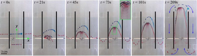
Figure 7: Pumping between parallel walls of distance $77$ mm. The blade reciprocates along the $x$-axis, and makes $90^{\circ}$ rotations near the walls. The blade’s angle of attack is $45^{\circ}$. The flow circulates from the side channels and returns to the central channel where the blade is moving.

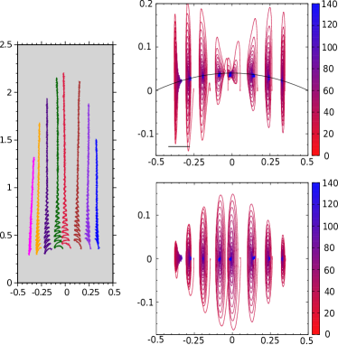
Figure 8: Image processing results for eight tracer particles. (a) Trajectories of floated polystyrene spheres in the central channel (different colors represent different spheres). They start their motions from the line $y=0.35W$. The blade reciprocates along the $x$-axis ($y=0$), and starts its motion from the leftmost endpoint. The initial zigzagging motion of tracers is due to wall effect, which diminishes at a distance $y\sim W$ from the blade’s location. (b) Evolution of the $v_{y}$ component of the velocity vector for eight tracer particles. Variable line colors indicate the elapsed time in seconds. It is seen that the velocities of particles along the central channel converge to Poiseuille profile with $v_{y}/v_{0}=0.04[1-(2x/W)^{2}]$ (note blue regions). The velocity oscillation is due to the zigzagging motion. (c) Same as panel b but for $v_{x}$, which gradually tends to zero for all particles.

IV The Pumping Function

We now operate the blade against two parallel separators of distance $W=77$ mm. Figure 7 shows the arrangement of the separators in the main rectangular container, and the location of the blade. Four sets of dyes have been introduced to the surface: two sets in side channels between the separators and container walls, and two rows in the main central channel on the two sides of the blade’s path (see Fig. 7, $t=0$). The blade is half-submerged and induces a surface flow. Since the central channel is connected to the side channels, we have a closed circuit for a possible free-surface flow. We actuate the blade with the same conditions as in our previous experiment. Figure 7 and Supplementary Material video 3 supp-videos show flow generation along the central and side channels. In contrast to the blade in infinite medium, where the streaming velocity drops as $\sim r^{-1}$, we find that the fluid velocity reaches a steady pattern along the channel. The blade sucks the fluid from the back side and pumps it forward. The zigzag footprint of the blade’s motion carried by traveling dyes (inset figure at $t=73$s) is similar to the head/tail-tip trajectory of wild-type C. elegans (see Fig. 1a in sznitman2010material ). Mixing is achieved over circulation time scale as fluid elements repeatedly revisit the blade. It is to be noted that the flow structure of a fixed blade imparting a net force is fundamentally different to that of a force free swimmer and here the the blade’s motion is inspired by the head movements of C. elegans.

We have floated polystyrene beads on the fluid surface and used their trajectories to measure the streaming velocity (Fig. 8). The velocity profile is Poiseuille and its maximum occurs along the centerline of the middle channel. We find $v_{\rm max}/v_{0}\approx 0.04$. The trajectories of the polystyrene tracers oscillate when they are close to the blade, but evolve into straight lines at a distance $y\sim W$. Initial zigzagging movements are due to wall effects: the moving blade induces two Stokeslet components, one parallel to the wall and the other normal to it. The normal component generates two side vortices lauga2005brownian which trap tracers until the parallel component pushes them out of the wall-induced vortices. The swimming efficiency of C. elegans is defined as $U/c$, where $U$ is the swimming speed and $c$ is the speed of bending waves. Similarly, the pumping efficiency in our mechanism can be defined as $v_{\rm max}/v_{0}$. Depending on its environment, C. elegans has a swimming efficiency of $0.08<U/c<0.15$ shen2011undulatory . The pumping efficiency in our experiments is about $4\%$. Therefore, a single blade’s pumping efficiency is quite comparable with the worm’s swimming efficiency, noting the fact that C. elegans gains thrust force from its tail, body and head segments ($U/c$ comes from at least three segments and not just from the head), and that $\Delta C$ in our experiments is relatively low because of adhesion effects.

A simple way to enhance the pumping efficiency is to increase the parameter $\Delta C$ by minimizing the adhesion between the fluid and the blade. In the ideal case with no-slip boundary condition at the blade’s surface, and when the blade is fully submerged, one obtains $\Delta C=8/3$ and the efficiency is expected to reach its maximum possible level of $0.14$.

We have not investigated the sensitivity of $v_{\rm max}/v_{0}$ to variations of $v_{0}$, $\omega_{0}$ and $W/D$ because of two limiting aspects of our setup: (i) decreasing $W/D$ connects the impenetrable layers of the blade and the wall due to adhesion effects and halts pumping (ii) increasing $v_{0}$ or $\omega_{0}$ generates large-amplitude surface waves and influences the dynamics of tracers. The blade cannot pump (as C. elegans cannot swim in highly viscous fluids) if either of its reciprocating or rotational motions is disabled. A flapping flexible blade, without translational motion, may still pump but the efficiency will be extremely low, and it will not have mixing capability. In sub-millimeter scales, the blade can be fabricated from magnetic materials and actuated remotely by an external, oscillating magnetic field. An implanted blade in an organ-on-a-chip device can perform the pumping function of the heart while simultaneously mixing and homogenizing the blood. In microprocessor technology, the blade can perform the role of a heat exchanger unit by pumping polymeric cooling liquid into a chamber and mixing heated and cooled streams as they reach the blade.

V Conclusion

In this manuscript, we created a low Reynold artificial mechanism with the goal of combining mixing and pumping functions into a single device, while each function requires a separate unit in the existing microfluidic devices. Inspired by the motion of C. elegans, which are evolved swimmers in highly viscous environments, we analyzed the motion of the head segment by approximating the head with a disk and breaking the motion into two stages of rocking and rotational movement. We showed that the blade’s motion not only mixes the surrounding fluid in a chaotic way, but also generates a steady Poiseuille flow with a pumping efficiency comparable with the swimming efficiency of the worm. We further showed that maximum efficiency actually occurs for the head motion of C. elegans, i.e., when the maximum disk angle is $45^{o}$ and the rocking and rotational stages follow a sinusoidal function with a $\pi/2$ phase difference. The pumping and mixing function resulted by the blade motion have potential applications in microfluidic devices such as microprocessors cooled by polymetric flows.

VI ACKNOWLEDGMENTS

This project was supported by the National Science Foundation under grant No. CMMI-1562871. The authors thank Leo Brossollet and Robert McKnight for their help in the initial development of the experimental setup. We would also like to thank the anonymous referees for valuable comments.

VII Appendix

Image processing method

A camera is installed under the corn syrup container facing upward. Red and blue food color dyes are injected in the liquid at its surface in order to track and quantize the liquid motion. Since the color dyes used in the experiment are much darker than the background liquid (i.e. corn syrup), wave frontier line is detected using color contrast. After converting the recorded video stream into a sequence of RGB frames, each color frame is transformed into a grayscale and then a binary image based on an appropriate threshold value to differentiate the dye frontier from the background liquid (the frontier appears in black while the background liquid turns into white in the binary image; see Fig. 9). To quantize the propulsion/pumping speed of the dye wave, the linear motion of the frontier wave center point is calculated and tracked. This point is the intersection of the perpendicular bisector of AB and the front wave (see Fig. 2 in the manuscript). While this point has an oscillating back and forth motion in short time scales due to rocking motion of the blade, its cycle average speed is always to the right (Fig. 9).

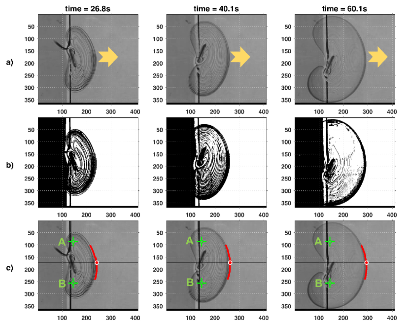
Figure 9: Three different snapshots show how the initial column of dye propagates by the blade’s motion. (a) Image extracted from the recorded video stream; (b) binary (i.e. black and white) conversion of the RGB image reveals the frontier of the dye wave; (c) edge of dye mixture is identified based on color contrast between the background liquid (corn syrup) and color dye.

Effect of Blade Angle and Rocking Velocity on Pumping (or Propulsion) Velocity

To investigate the effect of blade angle and rocking velocity on pumping performance, a set of experiments with different combination of blade angle and velocity is conducted. The results of two rocking velocities are shown in Fig. 10 and 11. For a given blade angle and rocking velocity, the pumping speed at a given location is a function of distance from the blade (denoted by $X$). As the front boarder moves away from the blade, its linear expansion rate decreases. Additionally, for a constant blade rocking velocity, the maximum expansion rate occurs at an optimal blade angle $\theta\approx 45^{\circ}$. As the rocking speed increases, the flow diverges from low Reynolds flow and, the maximum expansion rate happens at larger angles i.e. $\theta\approx 50^{\circ}$ (More details can be found in Fig. 11)

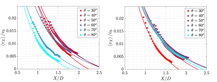
Figure 10: Effect of blade angle $\theta$ and rocking velocity $v_{0}$ on pumping speed. Different blade angles $\theta$ are tested for rocking speed (a) $v_{0}=4.87$cm/s; (b) $v_{0}=7.3$ cm/s. $D$ is the blade’s diameter.

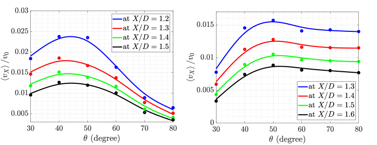
Figure 11: Maximum pumping speed at a given location $X/D$ versus blade angle $\theta$ for rocking velocity (a) $v_{0}=4.87$ cm/s, and (b) $v_{0}=7.3$ cm/s.

References

- (1) A. D. Stroock, S. K. Dertinger, A. Ajdari, I. Mezić, H. A. Stone, and G. M. Whitesides, Chaotic mixer for microchannels, Science 295, 647 (2002).
- (2) E. Gouillart, N. Kuncio, O. Dauchot, B. Dubrulle, S. Roux, and J.-L. Thiffeault, Walls inhibit chaotic mixing, Physical review letters 99, 114501 (2007).
- (3) A. S. Forouhar, M. Liebling, A. Hickerson, A. Nasiraei-Moghaddam, H.-J. Tsai, J. R. Hove, S. E. Fraser, M. E. Dickinson, and M. Gharib, The embryonic vertebrate heart tube is a dynamic suction pump, Science 312, 751 (2006).
- (4) J. Sznitman, P. K. Purohit, P. Krajacic, T. Lamitina, and P. E. Arratia, Material properties of caenorhabditis elegans swimming at low reynolds number, Biophysical journal 98, 617 (2010).
- (5) J. Gray and H. W. Lissmann, The locomotion of nematodes, Journal of Experimental Biology 41, 135 (1964).
- (6) G. J. Stephens, B. Johnson-Kerner, W. Bialek, and W. S. Ryu, Dimensionality and dynamics in the behavior of c. elegans, PLoS computational biology 4, e1000028 (2008).
- (7) R. Dreyfus, J. Baudry, M. L. Roper, M. Fermigier, H. A. Stone, and J. Bibette, Microscopic artificial swimmers, Nature 437, 862 (2005).
- (8) A. Shields, B. Fiser, B. Evans, M. Falvo, S. Washburn, and R. Superfine, Biomimetic cilia arrays generate simultaneous pumping and mixing regimes, Proceedings of the National Academy of Sciences (2010).
- (9) M. A. Jalali, A. Khoshnood, and M.-R. Alam, Microswimmer-induced chaotic mixing, Journal of Fluid Mechanics 779, 669 (2015).
- (10) M. Mirzakhanloo, M. A. Jalali, and M.-R. Alam, Hydrodynamic choreographies of microswimmers, Scientific reports 8, 3670 (2018).
- (11) M. Mirzakhanloo and M.-R. Alam, Flow characteristics of chlamydomonas result in purely hydrodynamic scattering, Physical Review E 98, 012603 (2018).
- (12) M. Backholm, A. Kasper, R. Schulman, W. Ryu, and K. Dalnoki-Veress, The effects of viscosity on the undulatory swimming dynamics of c. elegans, Physics of Fluids 27, 091901 (2015).
- (13) C. Fang-Yen, M. Wyart, J. Xie, R. Kawai, T. Kodger, S. Chen, Q. Wen, and A. D. Samuel, Biomechanical analysis of gait adaptation in the nematode caenorhabditis elegans, Proceedings of the National Academy of Sciences 107, 20323 (2010).
- (14) N. Cira, A. Benusiglio, and M. Prakash, Vapour-mediated sensing and motility in two-component droplets, Nature 519, 446 (2015).
- (15) Supplementary material: video 1 shows the time evolution of round dyes; video 2 presents the formation of circulatory streams on the two sides of the blade; video 3 demonstrates the flow generation along the central and side channels, See the Supplementary material at http://link.aps.org/supplemental/10.1103/PhysRevApplied.11.014065.
- (16) X. Shen and P. E. Arratia, Undulatory swimming in viscoelastic fluids, Physical review letters 106, 208101 (2011).
- (17) F. Hecht, New development in freefem++, Journal of numerical mathematics 20, 251 (2012).
- (18) M. A. Jalali, M.-R. Alam, and S. Mousavi, Versatile low-reynolds-number swimmer with three-dimensional maneuverability, Physical Review E 90, 053006 (2014).
- (19) J. Happel and H. Brenner, Low Reynolds number hydrodynamics: with special applications to particulate media, volume 1 (Springer Science & Business Media 2012).
- (20) Y. Ren and S. A. Barringer, Adhesion of sugar and oil solutions, Journal of food processing and preservation 33, 427 (2009).
- (21) G. Lapeyre, Characterization of finite-time lyapunov exponents and vectors in two-dimensional turbulence, Chaos: An Interdisciplinary Journal of Nonlinear Science 12, 688 (2002).
- (22) E. Lauga and T. M. Squires, Brownian motion near a partial-slip boundary: A local probe of the no-slip condition, Physics of Fluids 17, 103102 (2005).