Cyclotomic expansions of HOMFLY-PT colored by rectangular Young diagrams

Masaya Kameyama Satoshi Nawata Runkai Tao Hao Derrick Zhang
Abstract

We conjecture a closed-form expression of HOMFLY-PT invariants of double twist knots colored by rectangular Young diagrams where the twist is encoded in interpolation Macdonald polynomials. We also put forth a conjecture of cyclotomic expansions of HOMFLY-PT polynomials colored by rectangular Young diagrams for any knot.

1 Introduction

Colored HOMFLY-PT polynomials are two-variable quantum knot invariants associated with irreducible representations of $A_{N}$ type Lie algebras. Although several methods to compute HOMFLY-PT polynomials for arbitrary color in principle are known, carrying out explicit computation is practically very challenging for general non-torus knots and colors. However, in recent years, studying the structural properties of colored HOMFLY-PT polynomials, closed-form expressions for symmetric representations have been found for a certain class of non-torus knots.

Actually, the structural properties become more apparent at the level of HOMFLY-PT homology that categorifies quantum HOMFLY-PT polynomials. Lately, the HOMFLY-PT homology colored by arbitrary representations has been defined in [Cau17]. Although it is formidable to carry out computation of homology via the definition, various structural properties of HOMFLY-PT homology have been uncovered by combining mathematical definitions and physical predictions. In particular, it was proposed in [GGS18, GNS+16] that when colors are specified by rectangular Young diagrams, structural properties become more manifest if $(\mathbf{a,Q,t_{r},t_{c}})$ quadruple-grading is introduced.

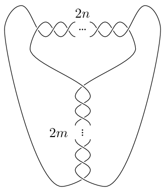
In [KM17], closed-form expressions of Poincare polynomials of HOMFLY-PT homology of the figure-eight and the trefoil colored by rectangular Young diagrams [rs]delimited-[]superscript๐‘Ÿ๐‘ [r^{s}] are conjectured. The conjectural formulas in [KM17] are very simple, being expressed by a summation over Young diagrams inscribed by [rs]delimited-[]superscript๐‘Ÿ๐‘ [r^{s}]. In this paper, we further generalize the formulas to the case of double twist knots drawn in Figure 1. Our conjectural formulas are expressed by a summation over iteratively inscribed Young diagrams with interpolation Macdonald polynomials, which can be understood as a generalization of cyclotomic expansions from symmetric representations [Hab08, NRZS12, GNS+16] to rectangular Young diagrams. We attach Mathematica files to arXiv page, which explicitly compute both HOMFLY-PT polynomials and Poincarรฉ polynomials of the double twist knots colored by rectangular Young diagrams. Like the Rosso-Jones formula [RJ93] for torus knots, we believe that the formulas will find many applications in other areas of mathematics.

Refer to caption

$$\begin{array}[]{c | c | c}m&n&\textrm{Name}\\ \hline\cr{1}&{1}&{3_{1}}\\ {-1}&{1}&{4_{1}}\\ {2}&{1}&{5_{2}}\\ {-2}&{1}&{6_{1}}\\ {3}&{1}&{7_{2}}\\ {2}&{2}&{7_{4}}\\ {-3}&{1}&{8_{1}}\\ {-2}&{2}&{8_{3}}\\ {4}&{1}&{9_{2}}\\ {3}&{2}&{9_{5}}\\ {-4}&{1}&{10_{1}}\\ {-3}&{2}&{10_{3}}\end{array}$$
Figure 1: Double twist knot $K_{m,n}$ and corresponding knots in Rolfsen Table up to 10 crossings.

Convention

Throughout this paper, we use the following skein relation for a reduced HOMFLY polynomial ${H}_{\Yboxdim{5pt}\yng(1)}(K;A,q)$:

Aโ€‹H\Yboxdimโ€‹5โ€‹pโ€‹tโ€‹\yngโ€‹(1)โ€‹([Uncaptioned image])โˆ’Aโˆ’1โ€‹H\Yboxdimโ€‹5โ€‹pโ€‹tโ€‹\yngโ€‹(1)โ€‹([Uncaptioned image])=(qโˆ’qโˆ’1)โ€‹H\Yboxdimโ€‹5โ€‹pโ€‹tโ€‹\yngโ€‹(1)โ€‹([Uncaptioned image]),๐ดsubscript๐ป\Yboxdim5๐‘๐‘ก\yng1[Uncaptioned image]superscript๐ด1subscript๐ป\Yboxdim5๐‘๐‘ก\yng1[Uncaptioned image]๐‘žsuperscript๐‘ž1subscript๐ป\Yboxdim5๐‘๐‘ก\yng1[Uncaptioned image]\displaystyle A~{}{H}_{\Yboxdim{5pt}\yng(1)}\left({\raisebox{-5.69046pt}{\includegraphics[width=17.07182pt]{overcrossing}}}\right)-A^{-1}{H}_{\Yboxdim{5pt}\yng(1)}\left({\raisebox{-5.69046pt}{\includegraphics[width=17.07182pt]{undercrossing}}}\right)=(q-q^{-1}){H}_{\Yboxdim{5pt}\yng(1)}\left({\raisebox{-5.69046pt}{\includegraphics[width=17.07182pt]{smoothing}}}\right)\,,

with the unknot invariant is normalized as

H\Yboxdimโ€‹5โ€‹pโ€‹tโ€‹\yngโ€‹(1)โ€‹([Uncaptioned image])=1.subscript๐ป\Yboxdim5๐‘๐‘ก\yng1[Uncaptioned image]1{H}_{\Yboxdim{5pt}\yng(1)}({\raisebox{-2.84544pt}{\includegraphics[width=11.38092pt]{unknot}}})=1~{}.

In addition, in this paper, a knot is always zero-framed and we do not consider non-trivial framings.

Acknowledgement

We would like to thank Alexei Morozov for discussion and correspondence. Without his help and encouragement, this paper would be impossible. S.N. would like to thank ICTS, KITP and IHES for warm hospitality where a part of work has been carried out. R.T. and H.D.Z. are grateful for the support from NSFC grant No.11850410428. This research was supported in part by the International Centre for Theoretical Sciences (ICTS) during a visit for participating in the program - Quantum Fields, Geometry and Representation Theory (Code: ICTS/qftgrt2018/07), and in part by the National Science Foundation under Grant No. NSF PHY-1748958 during a visit for participating in Quantum Knot Invariants and Supersymmetric Gauge Theories.

2 Colored HOMFLY-PT polynomials

It is conjectured in [KM17] that the [rs]delimited-[]superscript๐‘Ÿ๐‘ [r^{s}]-colored HOMFLY-PT polynomial of the figure-eight $K_{1,-1}$ is expressed as

H[rs]โ€‹(K1,โˆ’1;A,q)=โˆ‘ฮปโŠ‚[rs]Dฮป(s)โ€‹(q)โ€‹DฮปT(r)โ€‹(qโˆ’1)โ€‹โˆ\Yboxdimโ€‹5โ€‹pโ€‹tโ€‹\yngโ€‹(1)โˆˆฮป{Aโ€‹qr+a\Yboxdimโ€‹5โ€‹pโ€‹tโ€‹\yngโ€‹(1)โ€ฒโˆ’l\Yboxdimโ€‹5โ€‹pโ€‹tโ€‹\yngโ€‹(1)โ€ฒ}โ€‹{Aโ€‹qa\Yboxdimโ€‹5โ€‹pโ€‹tโ€‹\yngโ€‹(1)โ€ฒโˆ’l\Yboxdimโ€‹5โ€‹pโ€‹tโ€‹\yngโ€‹(1)โ€ฒโˆ’s},subscript๐ปdelimited-[]superscript๐‘Ÿ๐‘ subscript๐พ11๐ด๐‘žsubscript๐œ†delimited-[]superscript๐‘Ÿ๐‘ superscriptsubscript๐ท๐œ†๐‘ ๐‘žsuperscriptsubscript๐ทsuperscript๐œ†๐‘‡๐‘Ÿsuperscript๐‘ž1subscriptproduct\Yboxdim5๐‘๐‘ก\yng1๐œ†๐ดsuperscript๐‘ž๐‘Ÿsubscriptsuperscript๐‘Žโ€ฒ\Yboxdim5๐‘๐‘ก\yng1subscriptsuperscript๐‘™โ€ฒ\Yboxdim5๐‘๐‘ก\yng1๐ดsuperscript๐‘žsubscriptsuperscript๐‘Žโ€ฒ\Yboxdim5๐‘๐‘ก\yng1subscriptsuperscript๐‘™โ€ฒ\Yboxdim5๐‘๐‘ก\yng1๐‘ H_{[r^{s}]}(K_{1,-1};A,q)=\sum_{\lambda\subset[r^{s}]}D_{\lambda}^{(s)}(q)D_{\lambda^{T}}^{(r)}(q^{-1})\prod_{\Yboxdim{5pt}\yng(1)\in\lambda}\{Aq^{r+a^{\prime}_{\Yboxdim{5pt}\yng(1)}-l^{\prime}_{\Yboxdim{5pt}\yng(1)}}\}\{Aq^{a^{\prime}_{\Yboxdim{5pt}\yng(1)}-l^{\prime}_{\Yboxdim{5pt}\yng(1)}-s}\}\,,

where $\{x\}=x-x^{-1}$ and $\lambda^{T}$ is the transposition of $\lambda$. Here, the factor Dฮป(s)โ€‹(q)superscriptsubscript๐ท๐œ†๐‘ ๐‘žD_{\lambda}^{(s)}(q) is the principal specialization of the Schur polynomial

Dฮป(s)โ€‹(q):=sฮปโ€‹(qsโˆ’1,qsโˆ’3,โ€ฆ,qโˆ’s+3,qโˆ’s+1)=โˆ\Yboxdimโ€‹5โ€‹pโ€‹tโ€‹\yngโ€‹(1)โˆˆฮป{qsโˆ’l\Yboxdimโ€‹5โ€‹pโ€‹tโ€‹\yngโ€‹(1)โ€ฒ+a\Yboxdimโ€‹5โ€‹pโ€‹tโ€‹\yngโ€‹(1)โ€ฒ}{ql\Yboxdimโ€‹5โ€‹pโ€‹tโ€‹\yngโ€‹(1)+a\Yboxdimโ€‹5โ€‹pโ€‹tโ€‹\yngโ€‹(1)+1}.assignsuperscriptsubscript๐ท๐œ†๐‘ ๐‘žsubscript๐‘ ๐œ†superscript๐‘ž๐‘ 1superscript๐‘ž๐‘ 3โ€ฆsuperscript๐‘ž๐‘ 3superscript๐‘ž๐‘ 1subscriptproduct\Yboxdim5๐‘๐‘ก\yng1๐œ†superscript๐‘ž๐‘ subscriptsuperscript๐‘™โ€ฒ\Yboxdim5๐‘๐‘ก\yng1subscriptsuperscript๐‘Žโ€ฒ\Yboxdim5๐‘๐‘ก\yng1superscript๐‘žsubscript๐‘™\Yboxdim5๐‘๐‘ก\yng1subscript๐‘Ž\Yboxdim5๐‘๐‘ก\yng11D_{\lambda}^{(s)}(q):=s_{\lambda}(q^{s-1},q^{s-3},\ldots,q^{-s+3},q^{-s+1})=\prod_{\Yboxdim{5pt}\yng(1)\in\lambda}\frac{\{q^{s-l^{\prime}_{\Yboxdim{5pt}\yng(1)}+a^{\prime}_{\Yboxdim{5pt}\yng(1)}}\}}{\{q^{l_{\Yboxdim{5pt}\yng(1)}+a_{\Yboxdim{5pt}\yng(1)}+1}\}}~{}.

The formula is deduced by repackaging tedious calculations [Mor16] with the Cauchy formula

โˆi,j(1+xiโ€‹yi)=โˆ‘ฮปsฮปโ€‹(x)โ€‹sฮปTโ€‹(y),subscriptproduct๐‘–๐‘—1subscript๐‘ฅ๐‘–subscript๐‘ฆ๐‘–subscript๐œ†subscript๐‘ ๐œ†๐‘ฅsubscript๐‘ superscript๐œ†๐‘‡๐‘ฆ\prod_{i,j}\left(1+x_{i}y_{i}\right)=\sum_{\lambda}s_{\lambda}(x)s_{\lambda^{T}}(y)~{},

so that it naturally exhibits the exponential growth property of colored HOMFLY-PT polynomials [Zhu13] with respect to colors

$$H_{\lambda}(K;A,q=1)=\Big{[}H_{\Yboxdim{5pt}\yng(1)}(K;A,q=1)\Big{]}^{|\lambda|}~{},$$

where $|\lambda|$ is the number of boxes in $\lambda$. It is an elegant extension from symmetric representations [IMMM12] to rectangular Young diagrams. Hence, as in symmetric representations [NRZS12, GNS+16], one can expect that the [rs]delimited-[]superscript๐‘Ÿ๐‘ [r^{s}]-colored HOMFLY-PT polynomial of the double twist knot can be expressed by inserting an appropriate twist element into this formula.

Refer to caption
Figure 2: Convention
Refer to caption
Figure 3: Iteratively inscribed Young diagrams [rs]โŠƒฮป1โŠƒโ‹ฏโŠƒฮปmsuperset-ofdelimited-[]superscript๐‘Ÿ๐‘ subscript๐œ†1superset-ofโ‹ฏsuperset-ofsubscript๐œ†๐‘š[r^{s}]\supset\lambda_{1}\supset\cdots\supset\lambda_{m}.

In the case of symmetric representations, the twist element has been found from the $q$-binomial theorem. In fact, the binomial formula for any representation $\lambda$ is given in [Mac98, ยง3, Example 10]:

sฮปโ€‹(1+x1,1+x2,โ€ฆ,1+xn)=โˆ‘ฮผโŠ‚ฮปdฮปโ€‹ฮผโ€‹sฮผโ€‹(x1,โ€ฆ,xn)subscript๐‘ ๐œ†1subscript๐‘ฅ11subscript๐‘ฅ2โ€ฆ1subscript๐‘ฅ๐‘›subscript๐œ‡๐œ†subscript๐‘‘๐œ†๐œ‡subscript๐‘ ๐œ‡subscript๐‘ฅ1โ€ฆsubscript๐‘ฅ๐‘›s_{\lambda}\left(1+x_{1},1+x_{2},\ldots,1+x_{n}\right)=\sum_{\mu\subset\lambda}d_{\lambda\mu}s_{\mu}\left(x_{1},\ldots,x_{n}\right) (2.1)

where

$$d_{\lambda\mu}=\operatorname{det}\left(\left(\begin{array}[]{c}{\lambda_{i}+n-i}\\ {\mu_{j}+n-j}\end{array}\right)\right)_{1<i,j<n}~{}.$$

Thus, we use its $q$-deformation to define

Bฮป,ฮผ(s)โ€‹(A,q):=A2โ€‹|ฮผ|โ€‹q(1โˆ’s)โ€‹(|ฮป|โˆ’|ฮผ|)โ€‹(โˆ\Yboxdimโ€‹5โ€‹pโ€‹tโ€‹\yngโ€‹(1)โˆˆฮผq4โ€‹(a\Yboxdimโ€‹5โ€‹pโ€‹tโ€‹\yngโ€‹(1)โ€ฒโˆ’l\Yboxdimโ€‹5โ€‹pโ€‹tโ€‹\yngโ€‹(1)โ€ฒ))detโ€‹([ฮปi+sโˆ’iฮผj+sโˆ’j]q2)1โ‰คi,jโ‰คs.assignsuperscriptsubscript๐ต๐œ†๐œ‡๐‘ ๐ด๐‘žsuperscript๐ด2๐œ‡superscript๐‘ž1๐‘ ๐œ†๐œ‡subscriptproduct\Yboxdim5๐‘๐‘ก\yng1๐œ‡superscript๐‘ž4subscriptsuperscript๐‘Žโ€ฒ\Yboxdim5๐‘๐‘ก\yng1subscriptsuperscript๐‘™โ€ฒ\Yboxdim5๐‘๐‘ก\yng1detsubscriptsubscriptFRACOPsubscript๐œ†๐‘–๐‘ ๐‘–subscript๐œ‡๐‘—๐‘ ๐‘—superscript๐‘ž2formulae-sequence1๐‘–๐‘—๐‘ B_{\lambda,\mu}^{(s)}(A,q):=A^{2\absolutevalue{\mu}}q^{(1-s)(\absolutevalue{\lambda}-\absolutevalue{\mu})}\quantity(\prod_{\Yboxdim{5pt}\yng(1)\in\mu}q^{4(a^{\prime}_{\Yboxdim{5pt}\yng(1)}-l^{\prime}_{\Yboxdim{5pt}\yng(1)})})\ \ \textrm{det}\quantity({\lambda_{i}+s-i\brack\mu_{j}+s-j}_{q^{2}})_{1\leq i,j\leq s}\,. (2.2)

where ${x\brack y}_{q}$ is a $q$-binomial coefficient. Note that when $\mu=\emptyset$, we have Bฮป,โˆ…(s)=Dฮป(s)superscriptsubscript๐ต๐œ†๐‘ superscriptsubscript๐ท๐œ†๐‘ B_{\lambda,\emptyset}^{(s)}=D_{\lambda}^{(s)}. Using this, we introduce the following factor which admits two expressions

$\displaystyle F_{\lambda}^{(m)}(A,q)$ =(Dฮป(s))โˆ’1โ€‹โˆ‘ฮป=ฮป1โŠƒโ‹ฏโŠƒฮปmBฮป1,ฮป2(s)โ€‹Bฮป2,ฮป3(s)โ€‹โ‹ฏโ€‹Bฮปmโˆ’1,ฮปm(s)โ€‹Dฮปm(s)absentsuperscriptsuperscriptsubscript๐ท๐œ†๐‘ 1subscript๐œ†subscript๐œ†1superset-ofโ‹ฏsuperset-ofsubscript๐œ†๐‘šsuperscriptsubscript๐ตsubscript๐œ†1subscript๐œ†2๐‘ superscriptsubscript๐ตsubscript๐œ†2subscript๐œ†3๐‘ โ‹ฏsuperscriptsubscript๐ตsubscript๐œ†๐‘š1subscript๐œ†๐‘š๐‘ superscriptsubscript๐ทsubscript๐œ†๐‘š๐‘ \displaystyle=\quantity(D_{\lambda}^{(s)})^{-1}\sum_{\lambda=\lambda_{1}\supset\cdots\supset\lambda_{m}}B_{\lambda_{1},\lambda_{2}}^{(s)}B_{\lambda_{2},\lambda_{3}}^{(s)}\cdots B_{\lambda_{m-1},\lambda_{m}}^{(s)}D_{\lambda_{m}}^{(s)} (2.3)
$\displaystyle=\quantity(D_{\lambda^{T}}^{(r)})^{-1}\sum_{{\lambda^{T}}=\lambda^{\prime}_{1}\supset\cdots\supset\lambda^{\prime}_{m}}B_{\lambda^{\prime}_{1},\lambda^{\prime}_{2}}^{(r)}B_{\lambda^{\prime}_{2},\lambda^{\prime}_{3}}^{(r)}\cdots B_{\lambda^{\prime}_{m-1},\lambda^{\prime}_{m}}^{(r)}D_{\lambda^{\prime}_{m}}^{(r)}\Bigg{|}_{q\to q^{-1}}\,,$

where the summations are taken over iteratively inscribed Young diagrams as illustrated in Figure 3. Although the building blocks B(s)superscript๐ต๐‘ B^{(s)} and D(s)superscript๐ท๐‘ D^{(s)} depend on s๐‘ s in the first line, $F_{\lambda}^{(m)}(A,q)$ is a Laurent polynomial of $(A,q)$ independent of s(โ‰ฅlengthโ€‹(ฮป))annotated๐‘ absentlength๐œ†s(\geq\textrm{length}(\lambda)). In a similar fashion, $F_{\lambda}^{(m)}(A,q)$ is independent of $r(\geq\textrm{length}(\lambda^{T}))$ though each building block depends on $r$ in the second line. Note that $F^{m=1}_{\lambda}=1$ for any $\lambda$.

Using this, we define the twist element as

$\displaystyle\textrm{Tw}^{(m)}_{\lambda}(A,q):=\begin{cases}(-A^{2})^{\absolutevalue{\lambda}}\Big{(}\displaystyle\prod_{\Yboxdim{5pt}\yng(1)\in\lambda}q^{2a_{\Yboxdim{5pt}\yng(1)}-2l_{\Yboxdim{5pt}\yng(1)}}\Big{)}F^{(m)}_{\lambda}(A,q)\,,&m\in\mathbb{Z}_{>0}\,,\\ F^{(-m)}_{\lambda}(A^{-1},q^{-1})\,,&m\in\mathbb{Z}_{<0}\,.\end{cases}$ (2.4)

Then, we conjecture that the HOMFLY-PT polynomial of the double twist knot $K_{m,n}$ colored by a rectangular Young diagram [rs]delimited-[]superscript๐‘Ÿ๐‘ [r^{s}] is expressed as

H[rs]โ€‹(Km,n;A,q)=โˆ‘ฮปโŠ‚[rs]Twฮป(m)โ€‹Twฮป(n)Twฮป(1)โ€‹Twฮป(โˆ’1)โ€‹Dฮป(s)โ€‹(q)โ€‹DฮปT(r)โ€‹(qโˆ’1)โ€‹โˆ\Yboxdimโ€‹5โ€‹pโ€‹tโ€‹\yngโ€‹(1)โˆˆฮป{Aโ€‹qr+a\Yboxdimโ€‹5โ€‹pโ€‹tโ€‹\yngโ€‹(1)โ€ฒโˆ’l\Yboxdimโ€‹5โ€‹pโ€‹tโ€‹\yngโ€‹(1)โ€ฒ}โ€‹{Aโ€‹qa\Yboxdimโ€‹5โ€‹pโ€‹tโ€‹\yngโ€‹(1)โ€ฒโˆ’l\Yboxdimโ€‹5โ€‹pโ€‹tโ€‹\yngโ€‹(1)โ€ฒโˆ’s}.subscript๐ปdelimited-[]superscript๐‘Ÿ๐‘ subscript๐พ๐‘š๐‘›๐ด๐‘žsubscript๐œ†delimited-[]superscript๐‘Ÿ๐‘ subscriptsuperscriptTw๐‘š๐œ†subscriptsuperscriptTw๐‘›๐œ†subscriptsuperscriptTw1๐œ†subscriptsuperscriptTw1๐œ†superscriptsubscript๐ท๐œ†๐‘ ๐‘žsuperscriptsubscript๐ทsuperscript๐œ†๐‘‡๐‘Ÿsuperscript๐‘ž1subscriptproduct\Yboxdim5๐‘๐‘ก\yng1๐œ†๐ดsuperscript๐‘ž๐‘Ÿsubscriptsuperscript๐‘Žโ€ฒ\Yboxdim5๐‘๐‘ก\yng1subscriptsuperscript๐‘™โ€ฒ\Yboxdim5๐‘๐‘ก\yng1๐ดsuperscript๐‘žsubscriptsuperscript๐‘Žโ€ฒ\Yboxdim5๐‘๐‘ก\yng1subscriptsuperscript๐‘™โ€ฒ\Yboxdim5๐‘๐‘ก\yng1๐‘ H_{[r^{s}]}(K_{m,n};A,q)=\sum_{\lambda\subset[r^{s}]}\frac{\textrm{Tw}^{(m)}_{\lambda}\textrm{Tw}^{(n)}_{\lambda}}{\textrm{Tw}^{(1)}_{\lambda}\textrm{Tw}^{(-1)}_{\lambda}}D_{\lambda}^{(s)}(q)D_{\lambda^{T}}^{(r)}(q^{-1})\prod_{\Yboxdim{5pt}\yng(1)\in\lambda}\{Aq^{r+a^{\prime}_{\Yboxdim{5pt}\yng(1)}-l^{\prime}_{\Yboxdim{5pt}\yng(1)}}\}\{Aq^{a^{\prime}_{\Yboxdim{5pt}\yng(1)}-l^{\prime}_{\Yboxdim{5pt}\yng(1)}-s}\}\,. (2.5)

This is a natural extensions of the formulas for symmetric representations [NRZS12, GNS+16] to rectangular Young diagrams. We have checked this formula with the results in [KM16, Mor18b, Mor18a].


Motivated by this formula, we further generalize the conjecture of cyclotomic expansions of colored HOMFLY-PT polynomials of a knot $K$ for symmetric representations [KM15, Eqn.(2)], [NO16, Conjecture 2.3] to rectangular Young diagrams.

Conjecture 2.1 (Cyclotomic expansions).

Let $Y$ be a set of all Young diagrams. For a knot $K$, there exists a function

Cโ€‹(K):Yร—โ„ค>0โŸถโ„คโ€‹[Aยฑ,qยฑ];(ฮป,s)โ†ฆCฮป,sโ€‹(K;A,q),:๐ถ๐พformulae-sequenceโŸถ๐‘Œsubscriptโ„คabsent0โ„คsuperscript๐ดplus-or-minussuperscript๐‘žplus-or-minusmaps-to๐œ†๐‘ subscript๐ถ๐œ†๐‘ ๐พ๐ด๐‘žC(K):Y\times\mathbb{Z}_{>0}\longrightarrow\mathbb{Z}[A^{\pm},q^{\pm}]\ ;\ (\lambda,s)\mapsto C_{\lambda,s}(K;A,q)~{},

which satisfies the following properties

  • โ€ข

    Cโˆ…,sโ€‹(K;A,q)=1subscript๐ถ๐‘ ๐พ๐ด๐‘ž1C_{\emptyset,s}(K;A,q)=1 for any sโˆˆโ„ค>0๐‘ subscriptโ„คabsent0s\in\mathbb{Z}_{>0}

  • โ€ข

    Cฮป,sโ€‹(K;A,q)=0subscript๐ถ๐œ†๐‘ ๐พ๐ด๐‘ž0C_{\lambda,s}(K;A,q)=0 for s<lengthโ€‹(ฮป)๐‘ length๐œ†s<\textrm{length}(\lambda)

such that the [rs]delimited-[]superscript๐‘Ÿ๐‘ [r^{s}]-colored reduced HOMFLY-PT polynomial of the knot $K$ is expressed as

H[rs]โ€‹(K;A,q)subscript๐ปdelimited-[]superscript๐‘Ÿ๐‘ ๐พ๐ด๐‘ž\displaystyle H_{[r^{s}]}(K;A,q) $\displaystyle=$ (Aโˆ™โ€‹qโˆ™)rโ€‹sโ€‹โˆ‘ฮปโŠ‚[rs]Cฮป,sโ€‹(K;A,q)โ€‹DฮปT(r)โ€‹(qโˆ’1)โ€‹โˆ\Yboxdimโ€‹5โ€‹pโ€‹tโ€‹\yngโ€‹(1)โˆˆฮป{Aโ€‹qr+a\Yboxdimโ€‹5โ€‹pโ€‹tโ€‹\yngโ€‹(1)โ€ฒโˆ’l\Yboxdimโ€‹5โ€‹pโ€‹tโ€‹\yngโ€‹(1)โ€ฒ}.superscriptsuperscript๐ดโˆ™superscript๐‘žโˆ™๐‘Ÿ๐‘ subscript๐œ†delimited-[]superscript๐‘Ÿ๐‘ subscript๐ถ๐œ†๐‘ ๐พ๐ด๐‘žsuperscriptsubscript๐ทsuperscript๐œ†๐‘‡๐‘Ÿsuperscript๐‘ž1subscriptproduct\Yboxdim5๐‘๐‘ก\yng1๐œ†๐ดsuperscript๐‘ž๐‘Ÿsubscriptsuperscript๐‘Žโ€ฒ\Yboxdim5๐‘๐‘ก\yng1subscriptsuperscript๐‘™โ€ฒ\Yboxdim5๐‘๐‘ก\yng1\displaystyle(A^{\bullet}q^{\bullet})^{rs}\sum_{\lambda\subset[r^{s}]}C_{\lambda,s}(K;A,q)D_{\lambda^{T}}^{(r)}(q^{-1})\prod_{\Yboxdim{5pt}\yng(1)\in\lambda}\{Aq^{r+a^{\prime}_{\Yboxdim{5pt}\yng(1)}-l^{\prime}_{\Yboxdim{5pt}\yng(1)}}\}~{}. (2.6)

Importantly, Cฮป,sโ€‹(A,q)subscript๐ถ๐œ†๐‘ ๐ด๐‘žC_{\lambda,s}(A,q) is independent of $r$.

In fact, when a color is a symmetric reperesentation $\lambda=[r]$, (2.6) reduces to

$$H_{[r]}(K;A,q)=\left(A^{\bullet}q^{\bullet}\right)^{r}\sum_{r\geq k\geq 0}C_{k}(K;A,q)q^{-2rk}(A^{2}q^{2r};q^{2})_{k}{r\brack k}_{q^{2}}~{},$$

which is exactly equal to [NO16, Conjecture 2.3].

If we can make use of the transposition symmetry [Zhu13] of the colored HOMFLY-PT polynomials

$$H_{\lambda}(K;A,q)=H_{\lambda^{T}}(K;A,q^{-1})~{},$$

then the conjecture can be stated by exchanging $q\to q^{-1}$, sโ†’rโ†’๐‘ ๐‘Ÿs\to r and $\lambda\to\lambda^{T}$, but the details are omitted.

3 Poincarรฉ polynomials of colored HOMFLY-PT homology

In [KM17], it is further conjectured that Poincarรฉ polynomial of quadruply-graded HOMFLY-PT homology of the figure-eight colored by [rs]delimited-[]superscript๐‘Ÿ๐‘ [r^{s}] is given by

๐’ซ[rs]โ€‹(K1,โˆ’1;๐š,๐,๐ญ๐ซ,๐ญ๐œ)=โˆ‘ฮปโŠ‚[rs]๐”ปฮป(s)โ€‹(q,t)โ€‹๐”ปฮปT(r)โ€‹(tโˆ’1,qโˆ’1)โ€‹โˆ\Yboxdimโ€‹5โ€‹pโ€‹tโ€‹\yngโ€‹(1)โˆˆฮป{Aฯƒโ€‹qr+aโ–กโ€ฒโ€‹tโˆ’lโ–กโ€ฒ}โ€‹{Aโ€‹ฯƒโ€‹qaโ–กโ€ฒโ€‹tโˆ’sโˆ’lโ–กโ€ฒ}|(โ€‹3.1โ€‹)subscript๐’ซdelimited-[]superscript๐‘Ÿ๐‘ subscript๐พ11๐š๐subscript๐ญ๐ซsubscript๐ญ๐œevaluated-atsubscript๐œ†delimited-[]superscript๐‘Ÿ๐‘ superscriptsubscript๐”ป๐œ†๐‘ ๐‘ž๐‘กsuperscriptsubscript๐”ปsuperscript๐œ†๐‘‡๐‘Ÿsuperscript๐‘ก1superscript๐‘ž1subscriptproduct\Yboxdim5๐‘๐‘ก\yng1๐œ†๐ด๐œŽsuperscript๐‘ž๐‘Ÿsubscriptsuperscript๐‘Žโ€ฒโ–กsuperscript๐‘กsubscriptsuperscript๐‘™โ€ฒโ–ก๐ด๐œŽsuperscript๐‘žsubscriptsuperscript๐‘Žโ€ฒโ–กsuperscript๐‘ก๐‘ subscriptsuperscript๐‘™โ€ฒโ–กitalic-(3.1italic-)\mathscr{P}_{[r^{s}]}(K_{1,-1};\mathbf{a,Q,t_{r},t_{c}})=\sum_{\lambda\subset[r^{s}]}\mathbbm{D}_{\lambda}^{(s)}(q,t)\mathbbm{D}_{\lambda^{T}}^{(r)}(t^{-1},q^{-1})\prod_{\Yboxdim{5pt}\yng(1)\in\lambda}\{\frac{A}{\sigma}q^{r+a^{\prime}_{{}_{\square}}}t^{-l^{\prime}_{\square}}\}\{{A}{\sigma}q^{a^{\prime}_{{}_{\square}}}t^{-s-l^{\prime}_{{}_{\square}}}\}\bigg{|}_{\eqref{cov}}\,

where ๐”ปฮป(s)superscriptsubscript๐”ป๐œ†๐‘ \mathbbm{D}_{\lambda}^{(s)} is a principal specialization of the Macdonald polynomial

๐”ปฮป(s)โ€‹(q,t):=Pฮปโ€‹(tsโˆ’1,tsโˆ’3,โ€ฆ,tโˆ’s+3,tโˆ’s+1;q,t)=โˆ\Yboxdimโ€‹5โ€‹pโ€‹tโ€‹\yngโ€‹(1)โˆˆฮป{tsโˆ’lโ–กโ€ฒโ€‹qaโ–กโ€ฒ}{tlโ–ก+1โ€‹qaโ–ก},assignsuperscriptsubscript๐”ป๐œ†๐‘ ๐‘ž๐‘กsubscript๐‘ƒ๐œ†superscript๐‘ก๐‘ 1superscript๐‘ก๐‘ 3โ€ฆsuperscript๐‘ก๐‘ 3superscript๐‘ก๐‘ 1๐‘ž๐‘กsubscriptproduct\Yboxdim5๐‘๐‘ก\yng1๐œ†superscript๐‘ก๐‘ subscriptsuperscript๐‘™โ€ฒโ–กsuperscript๐‘žsubscriptsuperscript๐‘Žโ€ฒโ–กsuperscript๐‘กsubscript๐‘™โ–ก1superscript๐‘žsubscript๐‘Žโ–ก\mathbbm{D}_{\lambda}^{(s)}(q,t):=P_{\lambda}(t^{s-1},t^{s-3},\ldots,t^{-s+3},t^{-s+1};q,t)=\prod_{\Yboxdim{5pt}\yng(1)\in\lambda}\frac{\{t^{s-l^{\prime}_{{}_{\square}}}q^{a^{\prime}_{{}_{\square}}}\}}{\{t^{l_{{}_{\square}}+1}q^{a_{{}_{\square}}}\}}~{},

and the change of variables is

Aโ†’๐šโ€‹โˆ’๐ญ๐ซโ€‹๐ญ๐œ,tโ†’๐ญ๐ซโˆ’1,qโ†’โˆ’๐ญ๐œ,ฯƒโ†’๐ญ๐ซโˆ’sโ€‹๐โˆ’1.formulae-sequenceโ†’๐ด๐šsubscript๐ญ๐ซsubscript๐ญ๐œformulae-sequenceโ†’๐‘กsuperscriptsubscript๐ญ๐ซ1formulae-sequenceโ†’๐‘žsubscript๐ญ๐œโ†’๐œŽsuperscriptsubscript๐ญ๐ซ๐‘ superscript๐1A\to\mathbf{a\sqrt{-t_{r}t_{c}}},\quad t\to\mathbf{t_{r}}^{-1},\quad q\to-\mathbf{t_{c}},\quad\sigma\to\mathbf{t_{r}}^{-s}\mathbf{Q}^{-1}~{}. (3.1)

To find the corresponding twist element, we need the binomial theorem involving Macdonald polynomials. Happily, the binomial theorem has been generalized by using interpolation Macdonald polynomials $P_{\lambda}^{*}(x,q,t)$ [Oko97]. Some basics facts on this matter are summarized in Appendix A. Hence, motivated by the $(q,t)$-version (A.1) of the binomial theorem, we define the refined version of (2.2)

๐”นฮป,ฮผ(s)โ€‹(A,q,t):=assignsuperscriptsubscript๐”น๐œ†๐œ‡๐‘ ๐ด๐‘ž๐‘กabsent\displaystyle\mathbbm{B}_{\lambda,\mu}^{(s)}(A,q,t):= (โˆ’t(1โˆ’s))|ฮป|โˆ’|ฮผ|โ€‹(Aโ€‹qt)2โ€‹|ฮผ|โ€‹(โˆ\Yboxdimโ€‹5โ€‹pโ€‹tโ€‹\yngโ€‹(1)โˆˆฮปq2โ€‹a\Yboxdimโ€‹5โ€‹pโ€‹tโ€‹\yngโ€‹(1)โ€ฒโ€‹tโˆ’2โ€‹l\Yboxdimโ€‹5โ€‹pโ€‹tโ€‹\yngโ€‹(1)โ€ฒ)โ€‹(โˆ\Yboxdimโ€‹5โ€‹pโ€‹tโ€‹\yngโ€‹(1)โˆˆฮผq2โ€‹a\Yboxdimโ€‹5โ€‹pโ€‹tโ€‹\yngโ€‹(1)โ€ฒโ€‹tโˆ’2โ€‹l\Yboxdimโ€‹5โ€‹pโ€‹tโ€‹\yngโ€‹(1)โ€ฒ)superscriptsuperscript๐‘ก1๐‘ ๐œ†๐œ‡superscript๐ด๐‘ž๐‘ก2๐œ‡subscriptproduct\Yboxdim5๐‘๐‘ก\yng1๐œ†superscript๐‘ž2subscriptsuperscript๐‘Žโ€ฒ\Yboxdim5๐‘๐‘ก\yng1superscript๐‘ก2subscriptsuperscript๐‘™โ€ฒ\Yboxdim5๐‘๐‘ก\yng1subscriptproduct\Yboxdim5๐‘๐‘ก\yng1๐œ‡superscript๐‘ž2subscriptsuperscript๐‘Žโ€ฒ\Yboxdim5๐‘๐‘ก\yng1superscript๐‘ก2subscriptsuperscript๐‘™โ€ฒ\Yboxdim5๐‘๐‘ก\yng1\displaystyle(-t^{(1-s)})^{\absolutevalue{\lambda}-\absolutevalue{\mu}}\Big{(}\frac{Aq}{t}\Big{)}^{2\absolutevalue{\mu}}\Big{(}\prod_{\Yboxdim{5pt}\yng(1)\in\lambda}q^{2a^{\prime}_{\Yboxdim{5pt}\yng(1)}}t^{-2l^{\prime}_{\Yboxdim{5pt}\yng(1)}}\Big{)}\Big{(}\prod_{\Yboxdim{5pt}\yng(1)\in\mu}q^{2a^{\prime}_{\Yboxdim{5pt}\yng(1)}}t^{-2l^{\prime}_{\Yboxdim{5pt}\yng(1)}}\Big{)} (3.2)
$\displaystyle\times\frac{P_{\mu}^{*}(q^{2\lambda};q^{2},t^{2})}{P_{\mu}^{*}(q^{2\mu};q^{2},t^{2})}.\frac{P_{\lambda}^{*}(0;q^{-2},t^{-2})}{P_{\mu}^{*}(0;q^{-2},t^{-2})}~{}.$

In general, ๐”นฮป,ฮผ(s)superscriptsubscript๐”น๐œ†๐œ‡๐‘ \mathbbm{B}_{\lambda,\mu}^{(s)} is not a Laurent polynomial but a rational function, and ๐”นฮป,โˆ…(s)=๐”ปฮป(s)superscriptsubscript๐”น๐œ†๐‘ superscriptsubscript๐”ป๐œ†๐‘ \mathbbm{B}_{\lambda,\emptyset}^{(s)}=\mathbbm{D}_{\lambda}^{(s)}. Then, we introduce the factor

$\displaystyle\mathbbm{F}_{\lambda}^{(m)}(A,q,t)$ =(๐”ปฮป(s))โˆ’1โ€‹โˆ‘ฮป=ฮป1โŠƒโ‹ฏโŠƒฮปm๐”นฮป1,ฮป2(s)โ€‹๐”นฮป2,ฮป3(s)โ€‹โ‹ฏโ€‹๐”นฮปmโˆ’1,ฮปm(s)โ€‹๐”ปฮปm(s)absentsuperscriptsuperscriptsubscript๐”ป๐œ†๐‘ 1subscript๐œ†subscript๐œ†1superset-ofโ‹ฏsuperset-ofsubscript๐œ†๐‘šsuperscriptsubscript๐”นsubscript๐œ†1subscript๐œ†2๐‘ superscriptsubscript๐”นsubscript๐œ†2subscript๐œ†3๐‘ โ‹ฏsuperscriptsubscript๐”นsubscript๐œ†๐‘š1subscript๐œ†๐‘š๐‘ superscriptsubscript๐”ปsubscript๐œ†๐‘š๐‘ \displaystyle=\quantity(\mathbbm{D}_{\lambda}^{(s)})^{-1}\sum_{\lambda=\lambda_{1}\supset\cdots\supset\lambda_{m}}\mathbbm{B}_{\lambda_{1},\lambda_{2}}^{(s)}\mathbbm{B}_{\lambda_{2},\lambda_{3}}^{(s)}\cdots\mathbbm{B}_{\lambda_{m-1},\lambda_{m}}^{(s)}\mathbbm{D}_{\lambda_{m}}^{(s)} (3.3)
$\displaystyle=\quantity(\mathbbm{D}_{\lambda^{T}}^{(r)})^{-1}\sum_{{\lambda^{T}}=\lambda^{\prime}_{1}\supset\cdots\supset\lambda^{\prime}_{m}}\mathbbm{B}_{\lambda^{\prime}_{1},\lambda^{\prime}_{2}}^{(r)}\mathbbm{B}_{\lambda^{\prime}_{2},\lambda^{\prime}_{3}}^{(r)}\cdots\mathbbm{B}_{\lambda^{\prime}_{m-1},\lambda^{\prime}_{m}}^{(r)}\mathbbm{D}_{\lambda^{\prime}_{m}}^{(r)}\Bigg{|}_{q\leftrightarrow t^{-1}}\,.$

As in (2.3), it is independent of s(โ‰ฅlengthโ€‹(ฮป))annotated๐‘ absentlength๐œ†s~{}(\geq\textrm{length}(\lambda)) and $r~{}(\geq\textrm{length}(\lambda^{T}))$. Remarkably, even though each building block is a rational function of $(A,q,t)$, $\mathbbm{F}_{\lambda}^{(m)}$ is always a Laurent polynomial of $(A,q,t)$. We also observe that if $\textrm{length}(\lambda)\leq 2$, it is a Laurent polynomial with positive coefficients whereas it generally involves both positive and negative coefficients for $\textrm{length}(\lambda)>2$.

Finally, we conjecture that the Poincarรฉ polynomial of [rs]delimited-[]superscript๐‘Ÿ๐‘ [r^{s}]-colored HOMFLY-PT homology of the double twist knot $K_{m,n}$ can be expressed as

$\displaystyle\mathscr{P}_{[r^{s}]}(K_{m,n};\mathbf{a,Q,t_{r},t_{c}})=(-\mathbf{t_{r}}\mathbf{t_{c}})^{-rs(\textrm{sgn}(m)+\textrm{sgn}(n))/2}\times$ (3.4)
โˆ‘ฮปโŠ‚[rs]๐”ปฮป(s)โ€‹(q,t)โ€‹๐”ปฮปT(r)โ€‹(tโˆ’1,qโˆ’1)โ€‹โˆ\Yboxdimโ€‹5โ€‹pโ€‹tโ€‹\yngโ€‹(1)โˆˆฮป{Aฯƒโ€‹qr+aโ–กโ€ฒโ€‹tโˆ’lโ–กโ€ฒ}โ€‹{Aโ€‹ฯƒโ€‹qaโ–กโ€ฒโ€‹tโˆ’sโˆ’lโ–กโ€ฒ}|(โ€‹3.1โ€‹)โ€‹๐•‹โ€‹๐•จฮป(m)โ€‹๐•‹โ€‹๐•จฮป(n)๐•‹โ€‹๐•จฮป(1)โ€‹๐•‹โ€‹๐•จฮป(โˆ’1),evaluated-atsubscript๐œ†delimited-[]superscript๐‘Ÿ๐‘ superscriptsubscript๐”ป๐œ†๐‘ ๐‘ž๐‘กsuperscriptsubscript๐”ปsuperscript๐œ†๐‘‡๐‘Ÿsuperscript๐‘ก1superscript๐‘ž1subscriptproduct\Yboxdim5๐‘๐‘ก\yng1๐œ†๐ด๐œŽsuperscript๐‘ž๐‘Ÿsubscriptsuperscript๐‘Žโ€ฒโ–กsuperscript๐‘กsubscriptsuperscript๐‘™โ€ฒโ–ก๐ด๐œŽsuperscript๐‘žsubscriptsuperscript๐‘Žโ€ฒโ–กsuperscript๐‘ก๐‘ subscriptsuperscript๐‘™โ€ฒโ–กitalic-(3.1italic-)๐•‹subscriptsuperscript๐•จ๐‘š๐œ†๐•‹subscriptsuperscript๐•จ๐‘›๐œ†๐•‹subscriptsuperscript๐•จ1๐œ†๐•‹subscriptsuperscript๐•จ1๐œ†\displaystyle\sum_{\lambda\subset[r^{s}]}\mathbbm{D}_{\lambda}^{(s)}(q,t)\mathbbm{D}_{\lambda^{T}}^{(r)}(t^{-1},q^{-1})\prod_{\Yboxdim{5pt}\yng(1)\in\lambda}\{\frac{A}{\sigma}q^{r+a^{\prime}_{{}_{\square}}}t^{-l^{\prime}_{\square}}\}\{{A}{\sigma}q^{a^{\prime}_{{}_{\square}}}t^{-s-l^{\prime}_{{}_{\square}}}\}\bigg{|}_{\eqref{cov}}\,\frac{\mathbbm{T}\!\mathbbm{w}^{(m)}_{\lambda}\mathbbm{T}\!\mathbbm{w}^{(n)}_{\lambda}}{\mathbbm{T}\!\mathbbm{w}^{(1)}_{\lambda}\mathbbm{T}\!\mathbbm{w}^{(-1)}_{\lambda}}~{},

where the twist elements are defined as

$$\mathbbm{T}\!\mathbbm{w}^{(m)}_{\lambda}(\mathbf{a},\mathbf{t_{r}},\mathbf{t_{c}}):=\begin{cases}\Big{(}-\mathbf{a}^{2}\mathbf{t_{r}}^{2}\mathbf{t_{c}}^{2}\Big{)}^{\absolutevalue{\lambda}}\Big{(}\displaystyle\prod_{\Yboxdim{5pt}\yng(1)\in\lambda}\mathbf{t_{c}}^{2a_{\Yboxdim{5pt}\yng(1)}}\mathbf{t_{r}}^{2l_{\Yboxdim{5pt}\yng(1)}}\Big{)}\mathbbm{F}^{(m)}_{\lambda}(\mathbf{a},\mathbf{t_{c}},\mathbf{t_{r}})\,,&m\in\mathbb{Z}_{>0}\,,\\ \mathbbm{F}^{(-m)}_{\lambda}(\mathbf{a}^{-1},\mathbf{t_{c}}^{-1},\mathbf{t_{r}}^{-1})\,,&m\in\mathbb{Z}_{<0}\,.\end{cases}$$

Surprisingly, ๐’ซ[rs]โ€‹(Km,n)subscript๐’ซdelimited-[]superscript๐‘Ÿ๐‘ subscript๐พ๐‘š๐‘›\mathscr{P}_{[r^{s}]}(K_{m,n}) is a Laurent polynomial of $(\mathbf{a,Q,t_{r},t_{c}})$ with positive coefficients even though summands in (LABEL:final) are rational functions of $(\mathbf{a,Q,t_{r},t_{c}})$ in general. We have checked the structural properties [GGS18] such as self-symmetry, mirror symmetry, refined exponential growth property and colored differentials for a number of examples.

4 Discussion

The formulas conjectured in this paper cry out for geometric interpretation. In fact, the binomial theorem (2.1) can be interpreted by the first Chern class of the tensor product of vector bundles over a flag variety [Las82]. Recently, a new definition of the uncolored HOMFLY-PT homology is given by $(q,t)$-equivariant sheaves on Hilbert schemes of points on $\mathbb{C}^{2}$ [GNR16, OR18b, OR18a]. Although its colored version has yet to be defined, the formula in this paper strongly suggests that braiding on $(q,t)$-equivariant sheaves will be captured by interpolation Macdonald polynomials via the localization of equivariant Grothendieck-Riemann-Roch formula [Hai02] if it is defined.

The double twist knots can be obtained by taking surgeries on two components of Borromean rings with framings $-1/m$ and $-1/n$. Actually, the cyclotomic expansions of colored Jones polynomials of the double twist knots have been originally obtained from that of Borromean rings [Hab08]. Therefore the structure in this formula can be extended to Borromean rings and twist links at the level of colored HOMFLY-PT polynomials as in [Hab08, GNS+16]. In addition, it would be interesting to extract information about quantum $6j$-symbols with rectangular Young diagrams from the formula conjectured in this paper.

Although thirty years have passed since colored quantum knot invariants have been introduced, our understanding of colored invariants beyond symmetric representations is still very limited. The formula in this paper reveals deep mathematical structure hidden behind colored knot invariants, relating to special functions and potentially geometry. Of course, we just glimpse a tip of the iceberg, and we hope that our results will serve as a stepping stone toward the study of knot invariants of general colors.

Appendix A Interpolation Macdonald polynomials

In this โ€œAppendixโ€, we review a combinatorial definition of interpolation Macdonald polynomials introduced by [Sah96, Kno97, Oko98] and their binomial theorem [Oko97].

For a Young diagram $\lambda$, a Young tableau $T$ is obtained by filling the boxes of the Young diagram by the numbers in $\{1,...,n\}$. We denote the entry of a box by $T_{\Yboxdim{5pt}\yng(1)}$. A Young tableau is called a reverse tableau if the entries is weakly decreasing along each row and strongly decreasing along each column. The maximal number of entries in a reverse tableau must be not less than the length of the Young diagram by definition. A reverse tableau $T$ on $\lambda$ makes a sequence of Young diagrams

$$\emptyset\equiv\lambda^{(n)}\subseteq\lambda^{(n-1)}\subseteq\cdots\subseteq\lambda^{(0)}\equiv\lambda,$$

where $\lambda^{(k)}$ is the shape of a sub Young tableau of $T$ such that all entries satisfy $T_{\Yboxdim{5pt}\yng(1)}>k$. For example, if we consider the following reverse tableau on $\lambda=(4,4,3,2,2)$ with $n=6$

\Yboxdim

15pt \young(6662,5521,332,22,11)ย ,

then the sequence is

$${\Yboxdim 6pt\emptyset\subseteq\yng(3)\subseteq\yng(3,2)\subseteq\yng(3,2)\subseteq\yng(3,2,2)\subseteq\yng(4,3,3,2)\subseteq\yng(4,4,3,2,2)~{}.}$$

A skew Young diagram $\lambda/\mu$ is called horizontal strip if there is at most one box in each column of $\lambda$. For a horizontal strip $\lambda/\mu$, we denote sets of rows and columns intersecting with $\lambda/\mu$ by $R_{\lambda/\mu}$ and $C_{\lambda/\mu}$. Then, $R_{\lambda/\mu}-C_{\lambda/\mu}$ is a set of boxes belonging to $R_{\lambda/\mu}$ but not to $C_{\lambda/\mu}$. For the above sequence $\lambda^{(k-1)}/\lambda^{(k)}$ are horizontal strips for every $k=1,\ldots,6$. As an example, $\lambda^{(0)}/\lambda^{(1)}$ and $R_{\lambda^{(0)}/\lambda^{(1)}}-C_{\lambda^{(0)}/\lambda^{(1)}}$ correspond to the black boxes and the red box, respectively

\ytableausetup

boxsize=13pt {ytableau} *(white) &

*(red) *(black)

*(black) *(black)

Let $x=(x_{1},\ldots,x_{n})$ be $n$-tuple variables. The ordinary Macdonald polynomial $P_{\lambda}(x;q,t)$ is combinatorially defined as

$$P_{\lambda}(x;q,t)=\sum_{T}\psi_{T}(q,t)\prod_{\Yboxdim{5pt}\yng(1)\in\lambda}x_{T_{\Yboxdim{5pt}\yng(1)}}~{},$$

where the sum is taken over all reverse tableaux $T$ on $\lambda$ with entries in $\{1,\ldots,n\}$ and the coefficients $\psi_{T}(q,t)$ are defined by

$$\psi_{T}(q,t)=\prod_{i=1}^{n}\psi_{\lambda^{(i-1)}/\lambda^{(i)}}(q,t)~{},\quad\psi_{\lambda/\mu}(q,t)=\prod_{\Yboxdim{5pt}\yng(1)\in R_{\lambda/\mu}-C_{\lambda/\mu}}\frac{b_{\mu}(\Yboxdim{5pt}\yng(1))}{b_{\lambda}(\Yboxdim{5pt}\yng(1))}~{},$$

with

$$b_{\lambda}(\Yboxdim{5pt}\yng(1))=\frac{1-q^{a_{\Yboxdim{5pt}\yng(1)}}t^{l_{\Yboxdim{5pt}\yng(1)}+1}}{1-q^{a_{\Yboxdim{5pt}\yng(1)}+1}t^{l_{\Yboxdim{5pt}\yng(1)}}}~{}.$$

Then, the interpolation Macdonald polynomial $P_{\mu}^{*}(x;q,t)$ is combinatorially defined by

$$P_{\lambda}^{*}(x;q,t)=\sum_{T}\psi_{T}(q,t)\prod_{\Yboxdim{5pt}\yng(1)\in\mu}t^{1-T_{\Yboxdim{5pt}\yng(1)}}\left(x_{T_{\Yboxdim{5pt}\yng(1)}}-q^{a^{\prime}_{\Yboxdim{5pt}\yng(1)}}t^{-l^{\prime}_{\Yboxdim{5pt}\yng(1)}}\right).$$

Using the interpolation Macdonald polynomials, the binomial theorem is generalized [Oko97] to

$$\frac{P_{\lambda}^{*}\left(cx_{1},\ldots,cx_{n};q,t\right)}{P_{\lambda}^{*}(c,\ldots,c;q,t)}=\sum_{\mu}\frac{c^{|\mu|}}{t^{(n-1)|\mu|}}\frac{P_{\mu}^{*}\left(q^{-\lambda};q^{-1},t^{-1}\right)}{P_{\mu}^{*}\left(q^{-\mu};q^{-1},t^{-1}\right)}\frac{P_{\mu}^{*}\left(x_{n},\ldots,x_{1};q^{-1},t^{-1}\right)}{P_{\mu}^{*}(c,\ldots,c;q,t)}~{}.$$

In particular, the limit $c\to 0$ leads to

$$\frac{P_{\lambda}^{*}\left(x_{1},\ldots,x_{n};q,t\right)}{P_{\lambda}^{*}(0,\ldots,0;q,t)}=\sum_{\mu}\frac{P_{\mu}^{*}\left(q^{-\lambda};q^{-1},t^{-1}\right)}{P_{\mu}^{*}\left(q^{-\mu};q^{-1},t^{-1}\right)}\frac{P_{\mu}\left(x_{1},x_{2}t^{-1},\ldots,x_{n}t^{1-n};q,t\right)}{P_{\mu}^{*}(0,\ldots,0;q,t)}~{}.$$ (A.1)

If we restrict ourselves to the cases of symmetric representations and single variable $x_{1}$, this formula reduces to the usual $q$-binomial theorem.

References


Masaya Kameyama, Graduate School of Mathematics, Nagoya University, Nagoya 464-8602, Japan, m13020v@math.nagoya-u.ac.jp

Satoshi Nawata, Department of Physics and Center for Field Theory and Particle Physics, Fudan University, 2005 Songhu Road, 200438 Shanghai, China
Institut des Hautes ร‰tudes Scientifiques, 35 Route de Chartres, Bures-sur-Yvette, 91440, France

Kavli Institute for Theoretical Physics, Santa Barbara CA 93106, U.S.A., snawata@gmail.com

Runkai Tao, Department of Physics and Center for Field Theory and Particle Physics, Fudan University, 2005 Songhu Road, 200438 Shanghai, China, runkaitao@gmail.com

Hao Derrick Zhang, Department of Physics and Center for Field Theory and Particle Physics, Fudan University, 2005 Songhu Road, 200438 Shanghai, China, haozhangphys@gmail.com