Boundary integral equations for isotropic linear elasticity

Abstract

This articles first investigates boundary integral operators for the three-dimensional isotropic linear elasticity of a biphasic model with piecewise constant Lamé coefficients in the form of a bounded domain of arbitrary shape surrounded by a background material. In the simple case of a spherical inclusion, the vector spherical harmonics consist of eigenfunctions of the single and double layer boundary operators and we provide their spectra. Further, in the case of many spherical inclusions with isotropic materials, each with its own set of Lamé parameters, we propose an integral equation and a subsequent Galerkin discretization using the vector spherical harmonics and apply the discretization to several numerical test cases.

1 Introduction

We consider three-dimensional boundary value or interface problems of the isotropic elasticity equation related to the following operator:

$${\bf L}u:=-\mathop{\rm div}\Big{(}2\mu e(u)+\lambda\mathop{\rm Tr}\big{(}e(u)\big{)}\mathop{\rm Id}\Big{)},$$ (1.1)

where the strain tensor reads $e(u)={\frac{1}{2}}(\nabla u+\nabla u^{\top})$. It is obvious to see that the operator ${\bf L}$ is self-adjoint on $L^{2}(\mathbb{R}^{3})^{3}$.

In the definition of the operator (1.1), $\mu,\lambda\in\mathbb{R},\mu>0,2\mu+3\lambda>0$ are the so-called (constant) Lamé parameters. The parameter $\mu$ denotes the shear modulus which describes the tendency of the object to deform at a constant volume when being imposed with opposing forces. The other Lamé parameter $\lambda$ has no physical meanings but is introduced to simplify the definition of the operator (1.1). Indeed, it is related to the bulk modulus $K$ through the relation

$$\lambda=K-\frac{2}{3}\mu,$$

where the bulk modulus $K$ represents the object’s tendency to deform in all directions when acted on by opposing force from all directions. We refer to [12] for more detailed descriptions of the Lamé parameters. It is sometimes useful to introduce Poisson’s ratio $\nu$ which is defined by

$$\nu={\lambda\over 2(\mu+\lambda)},$$ (1.2)

and whose admissible range is $(-1,1/2)$. The material is extremely compressible in the limit $\nu\to-1$ while extremely incompressible in the other limit $\nu\to 1/2$ [18].

A model of linear elasticity with appropriate boundary conditions can be approximated by the classic finite element method, see for example [15, 19] just to name a few contributions from an abundant body of literature, for the general case with non-homogeneous source term. On the other hand, displacement fields $u$ being homogeneous solutions, i.e., ${\bf L}u=0$ within a given domain, can also be represented by isotropic elastic potentials [3, 13] and elasticity in piecewise constant isotropic media can then be treated as integral equations for specified interface conditions. At the origin of the integral formulation lies the definitions of layer potentials and their corresponding integral operators [3, 20] based on the Green’s function [1] in the context of the isotropic linear elasticity.

In particular, on a unit sphere, one can introduce the vector spherical harmonics forming an orthonormal basis of $[L^{2}(\mathbb{S}^{2})]^{3}$ and which are eigenfunctions of the corresponding double and single layer boundary operators based on the Green’s function [1] of isotropic linear elasticity. The vector spherical harmonics were introduced in [9, 10] as an extension of the scalar spherical harmonics [16, 23] to the vectorial case. They were further used in the discretization of different physical models such as the Navier-Stokes equations [8] or Maxwell’s equations [6, 2]. However, they are not widely used and only sparely reported in literature, in particular in the context of isotropic elasticity. We demonstrate in this article that the corresponding integral operators have interesting spectral properties which can be made explicit by employing the vector spherical harmonics.

Our main motivation for this work is the derivation of an integral equation to model elastic materials represented by piecewise constant Lamé constants with spherical inclusions following similar principles that were presented in [14, 4, 5] in the case of scalar diffusion. The particular choice of the vector spherical harmonics as basis functions for a Galerkin discretization thereof leads then to an efficient and stable numerical scheme by exploiting the spectral properties of the involved integral operators. A similar physical model was introduced in  [22] with an algebraic formula of the approximate solution. However, with the spectral properties of the layer potentials and integral operators at hand, our approach first introduces an integral formulation for the exact solution and thus a rigorous mathematical framework. In a second step, we then propose the Galerkin discretization. The mathematical framework lays out the basis to derive a rigorous error analysis which we plan in the future.

We summarize the main contributions and organization of this work as follows:

• In Section 2 and 3, we give an introduction and overview of the layer potentials and corresponding boundary integral operators of the isotropic linear elasticity operator (1.1) on an arbitrary bounded domain with Lipschitz boundary which are sparely reported in the literature.

• Analytical properties of layer potentials and boundary integral operators are presented and proven in Section 3.4.

• On the unit sphere, we introduce the vector spherical harmonics in Section 4 and prove spectral properties of the boundary operators and layer potentials of this particular basis.

• As an application, we consider a piecewise constant elastic model with spherical inclusions and derive a integral equation in Section 6 that is then discretized by means of the vector spherical harmonics and tested numerically in Section 7.

2 Preliminaries

Denote $\mathbb{S}^{2}$ the unit sphere and $B$ the unit ball in $\mathbb{R}^{3}$. Let throughout this paper $\Omega^{-}\subset\mathbb{R}^{3}$ denote a bounded domain with Lipschitz boundary $\Gamma=\partial\Omega^{-}$ and outward pointing normal vector field ${\bf n}:\Gamma\to\mathbb{S}^{2}$. Further, we denote by $\Omega^{+}$ the unbounded set $\mathbb{R}^{3}\backslash\overline{\Omega^{-}}$.

2.1 Notations

We will first introduce some standard notions in the context of integral equations which can be found in standard textbooks (see, for example, [17, 20, 21]).

Let $\Omega$ be a domain with Lipschitz boundary, e.g., $\Omega=\Omega^{-}$ or $\Omega=\Omega^{+}$ (unbounded). Following the conventions and notation of [20], we define for $s\in\mathbb{R}$

$$H_{\mathop{\rm loc}}^{s}(\Omega) =\left\{u\in\big{(}C_{\rm comp}^{\infty}(\Omega)\big{)}^{*}\;\middle|\;\forall\chi\in C_{\rm comp}^{\infty}(\Omega):\chi u\in H^{\ell}(\Omega)\right\},$$ (2.1)

see Definition 2.6.1 in [20], and note that this consist of a slightly unconventional definition of $H_{\mathop{\rm loc}}^{\ell}(\Omega)$, see also Remark 2.6.2. We further define, see Definition 2.6.5 in [20], for $s\in\mathbb{R}$

$$H_{\mathop{\rm comp}}^{s}(\Omega)=\bigcup\limits_{K}\left\{u\in H_{\mathop{\rm loc}}^{s}(\Omega)\;\middle|\;\mathop{\rm supp}(u)\subset K\right\},$$ (2.2)

where the union is taken over all relatively compact subsets $K\subset\Omega$, and introduce

$$V_{0}(\Omega^{-})=\left\{v\in H^{1}(\Omega^{-})\;\middle|\;\int_{\Omega^{-}}v=0\right\}.$$ (2.3)

Next, we denote by $H^{\frac{1}{2}}(\Gamma)^{3}$ the Sobolev space of order $\frac{1}{2}$ with the usual Sobolev-Slobodeckij norm $\|\lambda\|^{2}_{H^{\frac{1}{2}}(\Gamma)}:=\sum_{k=1}^{3}\|\lambda_{k}\|^{2}_{H^{\frac{1}{2}}(\Gamma)}$ for $\lambda=(\lambda_{1},\lambda_{2},\lambda_{3})^{\top}$ and with

$$\|\lambda_{k}\|^{2}_{H^{\frac{1}{2}}(\Gamma)}:=\|\lambda_{k}\|^{2}_{L^{2}(\Gamma)}+\int_{\Gamma}\int_{\Gamma}\frac{|\lambda_{k}(x)-\lambda_{k}(y)|^{2}}{|x-y|^{3}}\,dxdy.$$

Moreover, we define $H^{-\frac{1}{2}}(\Gamma)^{3}:=\left(H^{\frac{1}{2}}(\Gamma)^{3}\right)^{*}$ and we equip this Sobolev space with the canonical dual norm $\|\cdot\|_{H^{-\frac{1}{2}}(\Gamma)}$. We introduce

$$\gamma^{\mp}\colon H_{\mathop{\rm loc}}^{1}(\Omega^{\mp})^{3}\rightarrow H^{\frac{1}{2}}(\Gamma)^{3}$$ (2.4)

as the continuous, linear and surjective interior and exterior Dirichlet trace operators respectively, see Theorem 2.6.8 [20], and define the jump operator by

$$\llbracket\varphi\rrbracket=\gamma^{-}\varphi-\gamma^{+}\varphi.$$ (2.5)

Further, let $\gamma\colon H_{\mathop{\rm loc}}^{1}(\mathbb{R}^{3})^{3}\rightarrow H^{\frac{1}{2}}(\Gamma)^{3}$ be given by $\gamma\varphi=\gamma^{-}\varphi=\gamma^{+}\varphi$ almost everywhere.

Consider now the stress tensor $\mathcal{T}$ associate with ${\bf L}$, as is defined by (1.1), reading

$$\mathcal{T}\varphi:=2\mu e(\varphi)+\lambda\mathop{\rm Tr}e(\varphi)\mathop{\rm Id},\quad\varphi\in H^{1}_{\mathop{\rm loc}}(\Omega^{\mp})^{3}.$$ (2.6)

For the domains $\Omega^{\mp}$, the classical normal derivative operator, satisfying

$$\mathcal{T}^{\mp}_{\bf n}\varphi:=\gamma^{\mp}(\mathcal{T}\varphi{\bf n}),$$ (2.7)

for regular $\varphi$, can be extended to an operator $\mathcal{T}^{\mp}_{\bf n}:H^{1}_{\bf L}(\Omega^{\mp})^{3}\to H^{-\frac{1}{2}}(\Gamma)^{3}$, with $H^{1}_{\bf L}(\Omega)^{3}=\{u\in H^{1}(\Omega)^{3}\;|\;\mathbf{L}u\in L^{2}_{\mathop{\rm loc}}(\Omega)^{3}\}$, based on Green’s first identity. We then define the corresponding jump operator by

$$\llbracket\mathcal{T}\varphi\rrbracket=\mathcal{T}^{-}_{\bf n}\varphi-\mathcal{T}^{+}_{\bf n}\varphi.$$ (2.8)

Further, define $\mathcal{T}_{\bf n}:H^{1}_{\bf L}(\mathbb{R}^{3})^{3}\to H^{-\frac{1}{2}}(\Gamma)^{3}$ the global normal derivative operator given by $\mathcal{T}_{\bf n}\varphi=\mathcal{T}^{-}_{\bf n}\varphi=\mathcal{T}^{+}_{\bf n}\varphi$.

2.2 Fundamental solutions

Consider the matrix-valued fundamental solution $G=(G_{ij})_{ij}$ to the linear isotropic elasticity equation such that $G_{i}$, the $i$-th column of the matrix $G$ satisfies the following identity:

$${\bf L}G_{i}(x)=\delta(x)\,{\bf e}_{i},$$ (2.9)

with ${\bf L}$ defined by (1.1), $\delta$ being the Dirac distribution at the origin and ${\bf e}_{i}$ the canonical basis in $\mathbb{R}^{3}$. The Green’s function $G$ is given by [17, 21]:

$$G_{ij}(x):={1\over 8\pi\mu|x|}\left({\lambda+3\mu\over\lambda+2\mu}\delta_{ij}+{\lambda+\mu\over\lambda+2\mu}{x_{i}x_{j}\over|x|^{2}}\right),$$ (2.10)

where we recall that $\mu,\lambda$ are the Lamé constants and $\delta_{ij}$ is the Kronecker symbol.

2.3 Rigid displacement

For a given domain $\Omega\subset\mathbb{R}^{3}$, we consider the following problem: find $u\in H^{1}_{\mathop{\rm loc}}(\Omega)^{3}$ such that

$${\bf L}u=0,\quad\mbox{in}~{}H^{-1}(\Omega)^{3}$$ (2.11)

with appropriate boundary conditions. Equation (2.11) holds obviously if $e(u)=0$. Indeed, we call the displacement $u\in H^{1}_{\mathop{\rm loc}}(\Omega)^{3}$ a rigid displacement if $e(u)=0$. It is well-known that the displacement $u$ is a rigid displacement if and only if it has the form $u=Ax+b$ where $A\in\mathbb{R}^{3\times 3}$ is a constant skew matrix and $b\in\mathbb{R}^{3}$ a constant vector (see, for example, [11, 17]).

3 Layer potentials

In this section, we introduce the layer potentials and associated boundary operators which only have been sparsely reported in the literature for the operator ${\bf L}$. We therefore provide a complete overview.

3.1 Single layer potentials

Using the fundamental solution (2.10), we can now define the single layer potential $\mathcal{S}:H^{-\frac{1}{2}}(\Gamma)^{3}\to H^{1}(\mathbb{R}^{3}\textbackslash\Gamma)^{3}$ associated to the isotropic elasticity operator ${\bf L}$:

$$(\mathcal{S}\phi)(x):=\int_{\Gamma}G(x-y)\,\phi(y)\,dy,\quad x\in\mathbb{R}^{3}\textbackslash\Gamma.$$ (3.1)

Further, see e.g., [3], such function $\mathcal{S}\phi$ defined on $\mathbb{R}^{3}\textbackslash\Gamma$ is continuous across the interface $\Gamma$, i.e. $\llbracket\mathcal{S}\phi\rrbracket=0$ and a single layer boundary operator $\mathcal{V}:H^{-\frac{1}{2}}(\Gamma)^{3}\to H^{\frac{1}{2}}(\Gamma)^{3}$ can be defined by restricting the single layer potential to the boundary $\Gamma$:

$$(\mathcal{V}\phi)(x):=\int_{\Gamma}G(x-y)\,\phi(y)\,dy,\quad x\in\Gamma,$$ (3.2)

so that $\gamma\mathcal{S}\phi=\mathcal{V}\phi$. The following result is obvious:

Lemma 3.1.

For $\phi\in H^{-\frac{1}{2}}(\Gamma)^{3}$ and $\mathcal{S}\phi$ defined by (3.1), let ${\bf L}$ be the isotropic elasticity operator (1.1) and we have

$${\bf L}\mathcal{S}\phi=0\quad\mbox{in }\mathbb{R}^{3}\textbackslash\Gamma.$$

3.2 Double layer potential

We introduce the double layer potential $\mathcal{D}:H^{\frac{1}{2}}(\Gamma)^{3}\to H^{1}(\mathbb{R}^{3}\backslash\Gamma)^{3}$, by

$$\mathcal{D}\varphi(x)=\int_{\Gamma}\mathcal{T}_{{\bf n},y}(G)(x-y)\,\varphi(y)\,dy,\quad x\in\mathbb{R}^{3}\backslash\Gamma,$$ (3.3)

where the subscript $y$ means that the normal derivative operator $\mathcal{T}_{\bf n}$, defined in Section 2.1, is taken with respect to the $y$-variable. We define the double layer boundary operator $\mathcal{K}:H^{\frac{1}{2}}(\Gamma)^{3}\to H^{\frac{1}{2}}(\Gamma)^{3}$ by

$$(\mathcal{K}\varphi)(x)=\int_{\Gamma}\mathcal{T}_{{\bf n},y}(G)(x-y)\,\varphi(y)\,dy,\quad x\in\Gamma,$$ (3.4)

in the sense of principal value. Further, the adjoint double layer boundary operator $\mathcal{K}^{*}:H^{-\frac{1}{2}}(\Gamma)^{3}\to H^{-\frac{1}{2}}(\Gamma)^{3}$ is given as

$$(\mathcal{K}^{*}\phi)(x)=\int_{\Gamma}\left(\mathcal{T}_{{\bf n},x}(G)\right)^{\top}(x-y)\,\phi(y)\,dy,\quad x\in\Gamma,$$ (3.5)

Similar to Lemma 3.1, the following result is obvious:

Lemma 3.2.

For $\varphi\in H^{\frac{1}{2}}(\Gamma)^{3}$ and $\mathcal{D}\varphi$ defined by (3.3), we have

$${\bf L}\mathcal{D}\varphi=0\quad\mbox{in }\mathbb{R}^{3}\textbackslash\Gamma,$$

where ${\bf L}$ is the isotropic elasticity operator (1.1).

3.3 Newton potential

Finally, for sake of completeness, we also give the Newton potential associated to the isotropic elasticity operator (1.1). Define $\mathcal{N}:H_{\rm comp}^{s}(\mathbb{R}^{3})^{3}\to H_{\rm loc}^{s+2}(\mathbb{R}^{3})^{3}$ for $s\in\mathbb{R}$:

$$\mathcal{N}\psi(x)=\int_{\mathbb{R}^{3}}G(x-y)\psi(y)\,dy,\quad x\in\mathbb{R}^{3},$$ (3.6)

where $G$ is the Green’s function defined by (2.10). Following the definition for the elasticity operator ${\bf L}$ and all $\psi\in\mathcal{D}^{\prime}(\mathbb{R}^{3})^{3}$, we have

$$\psi={\bf L}\mathcal{N}\psi=\mathcal{N}{\bf L}\psi,\quad\mbox{in }\mathcal{D}^{\prime}(\mathbb{R}^{3})^{3}.$$ (3.7)

Let $\gamma^{*}:H^{-\frac{1}{2}}(\Gamma)^{3}\to H^{-1}_{\mathop{\rm comp}}(\mathbb{R}^{3})^{3}$, $\mathcal{T_{\bf n}}^{*}:H^{\frac{1}{2}}(\Gamma)^{3}\to H^{-1}_{\mathop{\rm comp}}(\mathbb{R}^{3}\textbackslash\Gamma)^{3}$ be the adjoint of the trace operator $\gamma$ and the adjoint of the normal derivative operator $\mathcal{T_{\bf n}}$ respectively, defined in Section 2.1. We then give an equivalent definition of the single and double layer potential:

$$\mathcal{S}=\mathcal{N}\gamma^{*},\quad\mathcal{D}=\mathcal{N}{\mathcal{T}_{\bf n}^{*}}.$$ (3.8)

3.4 Properties of layer potentials

We are now listing a selection of known results of layer potentials that will be used in the following. Let us first recall the following theorem given in [3] (see also [21, Section 6.7]):

Theorem 3.3.

Let $\phi\in H^{-\frac{1}{2}}(\Gamma)^{3}$ and the single layer potential $\mathcal{S}$, the adjoint double layer boundary operator $\mathcal{K}^{*}$ be defined by (3.1), (3.5) respectively. Then the interior and exterior normal traces of the stress tensor satisfy

$$\mathcal{T}_{\bf n}^{-}\mathcal{S}\phi={1\over 2}\phi+\mathcal{\mathcal{K}}^{*}\phi,\qquad\mathcal{T}_{\bf n}^{+}\mathcal{S}\phi=-{1\over 2}\phi+\mathcal{\mathcal{K}}^{*}\phi,\qquad\mbox{on }H^{-\frac{1}{2}}(\Gamma)^{3}.$$ (3.9)

We now show several jump conditions relating to the boundary layer potentials above which can be found, for example, in [17, Theorem 6.10].

Theorem 3.4.

Let $\Omega^{-}\in\mathbb{R}^{3}$ be a bounded Lipschitz domain with boundary $\Gamma$. Consider the single and double layer potentials defined by (3.1) and (3.3) respectively. Then it holds

$$\begin{array}[]{l}\llbracket\mathcal{S}\phi\rrbracket=0,\quad\llbracket\mathcal{D}\varphi\rrbracket=-\varphi,\quad\mbox{on }H^{\frac{1}{2}}(\Gamma)^{3},\\ \llbracket\mathcal{T}\mathcal{S}\phi\rrbracket=\phi,\quad\llbracket\mathcal{T}\mathcal{D}\varphi\rrbracket=0,\quad\mbox{on }H^{-\frac{1}{2}}(\Gamma)^{3}\end{array}$$ (3.10)

for all $\phi\in H^{-\frac{1}{2}}(\Gamma)^{3},\varphi\in H^{\frac{1}{2}}(\Gamma)^{3}$.

We now consider the invertibility of the single layer boundary operator (3.2) (see [17, Theorem 10.7] or [21, Theorem 6.36].

Lemma 3.5.

Let $\Omega^{-}\subset\mathbb{R}^{3}$ be a bounded domain with Lipschitz boundary $\Gamma$. If $\mu>0$ and $\lambda\geq 0$, the single layer boundary operator $\mathcal{V}$ defined by (3.2) is coercive, i.e.

$$\langle\mathcal{V}\phi,\phi\rangle_{H^{\frac{1}{2}}(\Gamma)\times H^{-\frac{1}{2}}(\Gamma)}>c\,\|\phi\|^{2}_{H^{-\frac{1}{2}}(\Gamma)},\qquad\forall\phi\in H^{-\frac{1}{2}}(\Gamma)^{3}.$$

Corollary 3.6 (Invertibility of the single layer boundary operator).

Let $\Omega^{-}\subset\mathbb{R}^{3}$ be a bounded domain with Lipschitz boundary $\Gamma$ and $\mu>0$ and $\lambda\geq 0$. Then, the single layer boundary operator $\mathcal{V}:H^{-\frac{1}{2}}(\Gamma)^{3}\to H^{\frac{1}{2}}(\Gamma)^{3}$ is invertible.

4 Real vector spherical harmonics

4.1 Surface gradient

In the following, we introduce the real vector spherical harmonics. We begin with some conventions of the gradient. On a given domain $\Omega$, consider a scalar valued function $f:\Omega\to\mathbb{R}^{3}$ and a column-vector valued function $F:\Omega\to\mathbb{R}^{3}$, we define their gradients by

$$\nabla f(x)\in\mathbb{R}^{3},~{}\mbox{with}~{}(\nabla f)_{i}={\partial f\over\partial x_{i}},\qquad\nabla F(x)\in\mathbb{R}^{3\times 3},~{}\mbox{with}~{}(\nabla F)_{ij}={\partial F_{i}\over\partial x_{j}}.$$ (4.1)

Note in particular that $\nabla f$ is a column-vector while $\nabla F$ are row-wise gradients for each component $F_{i}$.

Restricting the considerations to the unit ball $\Omega=B$ and it surface $\partial\Omega=\mathbb{S}^{2}$, we denote by

$$\nabla_{\!\rm s}=\hat{\theta}{\partial\over\partial\theta}+\hat{\phi}{1\over\sin\theta}{\partial\over\partial\phi}$$ (4.2)

the surface gradient operator and $\hat{r},\hat{\theta},\hat{\phi}$ are radial, polar and azimuthal unit vectors which are supposed to be row vectors. Let $f$ denote a scalar function and $F$ a vector-valued function, i.e. $f\in\mathbb{R}$ and $F\in\mathbb{R}^{3}$ and with the convention of the gradient field, the surface gradient (4.2) can alternatively be written as

$$\begin{array}[]{l}\nabla_{\!\rm s}f=\nabla f-{\bf n}({\bf n}^{\top}\nabla f),\\ \nabla_{\!\rm s}F=\nabla F-(\nabla F{\bf n}){\bf n}^{\top},\\ \end{array}$$ (4.3)

where $\nabla$ is the gradient in $\mathbb{R}^{3}$ based on the convention (4.1). It is immediate to verify that

$$\nabla_{\!\rm s}f^{\top}{\bf n}=0,\quad\nabla_{\!\rm s}F{\bf n}=0.$$

4.2 Definition of vector spherical harmonics

The construction of the vector spherical harmonics is based on the scalar real spherical harmonics defined on the unit sphere $\mathbb{S}^{2}$ denoted by $(Y_{\ell m})_{l\geq 0}^{|m|\leq\ell}$ which are normalized such that

$$\langle Y_{\ell m},Y_{\ell^{\prime}m^{\prime}}\rangle_{\mathbb{S}^{2}}=\int_{\mathbb{S}^{2}}Y_{\ell m}Y_{\ell^{\prime}m^{\prime}}=\delta_{\ell\ell^{\prime}}\delta_{m^{\prime}m^{\prime}}.$$

The vector spherical harmonics $V_{\ell m},W_{\ell m},X_{\ell m}:\mathbb{S}^{2}\to\mathbb{R}^{3}$ of degree $\ell\geq 0$ and order $m$, $|m|\leq\ell$ are given by

$$V_{\ell m}:=\nabla_{\!\rm s}Y_{\ell m}(\theta,\phi)-(\ell+1)Y_{\ell m}(\theta,\phi)\hat{r},$$ (4.4)

$$W_{\ell m}:=\nabla_{\!\rm s}Y_{\ell m}(\theta,\phi)+\ell Y_{\ell m}(\theta,\phi)\hat{r},$$

$$X_{\ell m}:=\hat{r}\times\nabla_{\!\rm s}Y_{\ell m}(\theta,\phi).$$

The symbol $\times$ represents the cross product in $\mathbb{R}^{3}$. We refer to Appendix A for some explicit expressions of the vector spherical harmonics for the first few degrees. The vector spherical harmonics satisfy the following orthogonal properties:

$$\int_{\mathbb{S}^{2}}V_{\ell m}\cdot W_{\ell^{\prime}m^{\prime}}=0,~{}\int_{\mathbb{S}^{2}}W_{\ell m}\cdot X_{\ell^{\prime}m^{\prime}}=0,~{}\int_{\mathbb{S}^{2}}X_{\ell m}\cdot V_{\ell^{\prime}m^{\prime}}=0,$$ (4.5)

$$\int_{\mathbb{S}^{2}}V_{\ell m}\cdot V_{\ell^{\prime}m^{\prime}}=\delta_{\ell\ell^{\prime}}\delta_{m^{\prime}m^{\prime}}(\ell+1)(2\ell+1),~{}\int_{\mathbb{S}^{2}}W_{\ell m}\cdot W_{\ell^{\prime}m^{\prime}}=\delta_{\ell\ell^{\prime}}\delta_{m^{\prime}m^{\prime}}\ell(2\ell+1),$$

$$\int_{\mathbb{S}^{2}}X_{\ell m}\cdot X_{\ell^{\prime}m^{\prime}}=\delta_{\ell\ell^{\prime}}\delta_{m^{\prime}m^{\prime}}\ell(\ell+1).$$

The scalar spherical harmonics (and thus the vector spherical harmonics) can be extended to any sphere $\Gamma_{r}(x_{0})=\partial B_{r}(x_{0})$ by translation and scaling. We will introduce the following scaled scalar product on $\Gamma_{r}(x_{0})$ given by

$$\langle u,v\rangle_{\Gamma_{r}(x_{0})}={1\over r^{2}}\int_{\Gamma_{r}(x_{0})}u(s)\cdot v(s)ds=\int_{\mathbb{S}^{2}}u(x_{0}+rs^{\prime})\cdot v(x_{0}+rs^{\prime})ds^{\prime}.$$ (4.6)

In practice, the exact value of the scalar product (4.6) cannot be computed explicitly in general. With a set $\{s_{t},w_{t}\}_{t=1}^{T_{g}}$ of integration points and weights on the unit sphere, the scalar product is approximated by the quadrature rule

$$\langle u,v\rangle_{\Gamma_{r}(x_{0}),t}=\sum\limits_{t=1}^{T_{g}}w_{t}\,u(x_{0}+rs_{t})\cdot v(x_{0}+rs_{t}).$$ (4.7)

In the numerical tests below in Section 7, we will use the Lebedev quadrature points  [7], which have the property that scalar spherical harmonics up to a certain degree $N_{g}$ are integrated exactly. This relationship is displayed in Table 1. It can be noticed that the number of points increases quadratically with $N_{g}$.

Further, the family of vector spherical harmonics gives a complete basis of $L^{2}(\Gamma_{r}(x_{0}))^{3}$ and any real function $f\in L^{2}(\Gamma_{r}(x_{0}))^{3}$ can be represented as

$$f(x)=\sum\limits_{\ell=0}^{\infty}\sum\limits_{m=-\ell}^{\ell}[v]_{\ell m}V_{\ell m}\Big{(}{x-x_{0}\over r}\Big{)}+[w]_{\ell m}W_{\ell m}\Big{(}{x-x_{0}\over r}\Big{)}+[x]_{\ell m}X_{\ell m}\Big{(}{x-x_{0}\over r}\Big{)},$$ (4.8)

where $[v]_{\ell m},[w]_{\ell m},[x]_{\ell m}\in\mathbb{R}$.

$N_{g}$	3	5	7	9	11	13	15	17	19	21	23	25	27	29
$T_{g}$	6	14	26	38	50	74	86	110	146	170	194	230	266	302
$N_{g}$	31	35	41	47	53	59	65	71	77	83	89	95	101	107
$T_{g}$	350	434	590	770	974	1202	1454	1730	2030	2354	2702	3074	3470	3890

Table 1: Degree $N_{g}$ and number of points $T_{g}$ of Lebedev quadrature rules such that spherical haromonics up to degree $N_{g}$ are integrated exactly with $T_{g}$ points.

4.3 Properties of the derivatives

We give some derivative properties of the surface gradient (4.3) that shall be useful in the upcoming analysis. In the following, let $u$ be the a scalar-valued function, $F,G$ be vector-valued functions and ${\bf A}$ be a matrix-valued function. We have the following product rule:

$$\begin{array}[]{l}\nabla_{\!\rm s}(uF)=F\nabla_{\!\rm s}u^{\top}+u\nabla_{\!\rm s}F,\\ \nabla_{\!\rm s}(F^{\top}G)=\nabla_{\!\rm s}F^{\top}G+\nabla_{\!\rm s}G^{\top}F.\end{array}$$ (4.9)

We also have the property for the cross product:

$$\nabla_{\!\rm s}(F\times G)=\nabla_{\!\rm s}F\times G-\nabla_{\!\rm s}G\times F.$$ (4.10)

Later proof also requires the triple product

$$\big{(}{\bf A}\times F\big{)}^{\top}G={\bf A}^{\top}\big{(}F\times G\big{)}=\big{(}G\times{\bf A}\big{)}^{\top}F.$$ (4.11)

Now let $h=h(r)$ be a scalar function which does not depend on the polar angles and $u=u(\theta,\phi),H=H(\theta,\phi)$ a scalar and a vector valued function respectively depending only on the polar angles. Then there holds

$$\begin{array}[]{l}\nabla(hu)=h_{r}u\hat{r}+{1\over r}h\nabla_{\!\rm s}u,\\ \nabla(hH)=h_{r}H\hat{r}^{\top}+{1\over r}h\nabla_{\!\rm s}H.\end{array}$$ (4.12)

For the scalar function $h=h(r)$, denote by $h_{r},h_{rr}$ the first and second derivative. Then we have

$$\mathop{\rm div}(hV_{\ell m})=-(\ell+1)\Big{(}h_{r}+{\ell+2\over r}h\Big{)}Y_{\ell m},$$ (4.13)

$$\mathop{\rm div}(hW_{\ell m})=\ell\Big{(}h_{r}-{\ell-1\over r}h\Big{)}Y_{\ell m},$$

$$\mathop{\rm div}(hX_{\ell m})=0,$$

and

$$\Delta(hV_{\ell m})=\Big{(}h_{rr}+{2\over r}h_{r}-{(\ell+1)(\ell+2)\over r^{2}}h\Big{)}V_{\ell m},$$ (4.14)

$$\Delta(hW_{\ell m})=\Big{(}h_{rr}+{2\over r}h_{r}-{(\ell-1)\ell\over r^{2}}h\Big{)}W_{\ell m},$$

$$\Delta(hX_{\ell m})=\Big{(}h_{rr}+{2\over r}h_{r}-{\ell(\ell+1)\over r^{2}}h\Big{)}X_{\ell m}.$$

Equations (4.13), (4.14) are given in [9]. Finally, the following identities hold, resulting directly from the definition of the vector spherical harmonics:

$$\nabla_{\!\rm s}Y_{\ell m}={1\over 2\ell+1}(\ell V_{\ell m}+(\ell+1)W_{\ell m}),\quad Y_{\ell m}\hat{r}={1\over 2\ell+1}(W_{\ell m}-V_{\ell m}).$$ (4.15)

5 Spectral properties of the layer potentials

We will give the main results in Section 5.1, prepare some preliminary results in Section 5.2 and finally provide the proofs in Section 5.3.

5.1 Main results

Consider the single layer potential $\mathcal{S}$ and the single layer boundary operator $\mathcal{V}$ defined by (3.1) and (3.2), we have the following result.

Theorem 5.1.

Let $\underline{Y_{\ell m}}$ be the matrix such that

$$\underline{Y_{\ell m}}=(V_{\ell m}|W_{\ell m}|X_{\ell m}):=(Y_{\ell m}^{1}|Y_{\ell m}^{2}|Y_{\ell m}^{3}).$$ (5.1)

Then we have:

1. On the unit sphere $\mathbb{S}^{2}$,

   $$\mathcal{V}\underline{Y_{\ell m}}(x)=\underline{Y_{\ell m}}A_{\mathcal{V},\ell},$$

   where $\mathcal{V}$ is the single layer boundary operator defined by (3.2) and $A_{\mathcal{V},\ell}$ is a constant matrix given by

   $$A_{\mathcal{V},\ell} =\begin{bmatrix}{(3\ell+1)\mu+\ell\lambda\over(2\ell+3)(2\ell+1)\mu(2\mu+\lambda)}&0&0\\ 0&{(3\ell+2)\mu+(\ell+1)\lambda\over(2\ell-1)(2\ell+1)\mu(2\mu+\lambda)}&0\\ 0&0&{1\over\mu(2\ell+1)}\end{bmatrix}=\mathop{\rm diag}(\tau_{\mathcal{V},\ell}^{1},\tau_{\mathcal{V},\ell}^{2},\tau_{\mathcal{V},\ell}^{3}).$$ (5.2)

2. When $|x|<1$, we have

   $$(\mathcal{S}\underline{Y_{\ell m}})(x)=\underline{Y_{\ell m}}\left({x\over|x|}\right)A_{\mathcal{S},\ell}^{in}(x),$$

   where $\mathcal{S}$ is the single layer potential given by (3.1) and the matrix $A_{\mathcal{S},\ell}^{in}(x)$ has the form

   $$A_{\mathcal{S},\ell}^{in}(x)=\begin{bmatrix}{(3\ell+1)\mu+\ell\lambda\over(2\ell+3)(2\ell+1)\mu(2\mu+\lambda)}|x|^{\ell+1}&0&0\\ {(\ell+1)(\mu+\lambda)\over 2(2\ell+1)\mu(2\mu+\lambda)}(|x|^{\ell+1}-|x|^{\ell-1})&{(3\ell+2)\mu+(\ell+1)\lambda\over(2\ell-1)(2\ell+1)\mu(2\mu+\lambda)}|x|^{\ell-1}&0\\ 0&0&{1\over(2\ell+1)\mu}|x|^{\ell}\end{bmatrix}.$$ (5.3)

3. When $|x|>1$, we have

   $$(\mathcal{S}\underline{Y_{\ell m}})(x)=\underline{Y_{\ell m}}\left({x\over|x|}\right)A_{\mathcal{S},\ell}^{out}(x),$$

   where the matrix $A_{\mathcal{S},\ell}^{out}(x)$ is given by

   $$A_{\mathcal{S},\ell}^{out}(x)=\begin{bmatrix}{(3\ell+1)\mu+\ell\lambda\over(2\ell+3)(2\ell+1)\mu(2\mu+\lambda)}|x|^{-\ell-2}&{\ell(\mu+\lambda)\over 2(2\ell+1)\mu(2\mu+\lambda)}(|x|^{-\ell-2}-|x|^{-\ell})&0\\ 0&{(3\ell+2)\mu+(\ell+1)\lambda\over(2\ell-1)(2\ell+1)\mu(2\mu+\lambda)}|x|^{-\ell}&0\\ 0&0&{1\over(2\ell+1)\mu}|x|^{-\ell-1}\end{bmatrix}.$$ (5.4)

The following result is a corollary of Theorem 5.1.

Corollary 5.2.

Let $\underline{Y_{\ell m}}$ be the a matrix defined by (5.1). Then, on the unit sphere $\mathbb{S}^{2}$, there holds

$$\mathcal{K}^{*}\underline{Y_{\ell m}}=\mathcal{K}\underline{Y_{\ell m}}=\underline{Y_{\ell m}}A_{\mathcal{K}^{*},\ell},$$

where $\mathcal{K}$ is the double layer boundary operator (3.5) with its adjoint $\mathcal{K}^{*}$ and $A_{\mathcal{K}^{*},\ell}$ is a constant and diagonal matrix:

$$A_{\mathcal{K}^{*},\ell}=\begin{bmatrix}-{2(2\ell^{2}+6\ell+1)\mu-3\lambda\over 2(2\ell+1)(2\ell+3)(2\mu+\lambda)}&0&0\\ 0&{2(2\ell^{2}-2\ell-3)\mu-3\lambda\over 2(2\ell+1)(2\ell-1)(2\mu+\lambda)}&0\\ 0&0&{1\over 2\mu(2\ell+1)}\end{bmatrix}=\mathop{\rm diag}(\tau_{\mathcal{K}^{*},\ell}^{1},\tau_{\mathcal{K}^{*},\ell}^{2},\tau_{\mathcal{K}^{*},\ell}^{3}).$$ (5.5)

Remark 5.3.

Recall that the Lamé constats $\mu,\lambda$ satisfy $\mu>0,2\mu+3\lambda>0$, we can verify that the eigenvalue $\tau_{\mathcal{K}^{*},\ell}^{k}$ of the adjoint double layer boundary operator is $-{1\over 2}$ if and only if $\ell=1,k=2$. And the eigenvectors associated with the eigenvalue $-{1\over 2}$ are $W_{1m}$, $m=\pm 1,0$.

The following theorem gives explicit expressions of the double layer potential.

Theorem 5.4.

Let $\underline{Y_{\ell m}}$ be given by (5.1) and $\mathcal{D}$ the double layer potential on the unit sphere introduced in (3.3), we have:

1. For $|x|<1$,

   $$(\mathcal{D}\underline{Y_{\ell m}})(x)=\underline{Y_{\ell m}}\Big{(}{x\over|x|}\Big{)}A_{\mathcal{D},\ell}^{in}(x)$$

   where

   $$A_{\mathcal{D},\ell}^{in}(x)=\begin{bmatrix}a^{in,\mathcal{D},\ell}_{11}|x|^{\ell+1}&a^{in,\mathcal{D},\ell}_{12}|x|^{\ell+1}&0\\ a^{in,\mathcal{D},\ell}_{21,1}|x|^{\ell+1}+a^{in,\mathcal{D},\ell}_{21,2}|x|^{\ell-1}&a^{in,\mathcal{D},\ell}_{22,1}|x|^{\ell+1}+a^{in,\mathcal{D},\ell}_{22,2}|x|^{\ell-1}&0\\ 0&0&-{\ell+1\over(2\ell+1)\mu}|x|^{\ell}\end{bmatrix}.$$ (5.6)

2. For $|x|>1$,

   $$(\mathcal{D}\underline{Y_{\ell m}})(x)=\underline{Y_{\ell m}}\Big{(}{x\over|x|}\Big{)}A_{\mathcal{D},\ell}^{out}(x)$$

   where

   $$A_{\mathcal{D},\ell}^{out}(x)=\begin{bmatrix}a^{out,\mathcal{D},\ell}_{11,1}|x|^{-\ell-2}+a^{out,\mathcal{D},\ell}_{11,2}|x|^{-\ell}&a^{out,\mathcal{D},\ell}_{12,1}|x|^{-\ell-2}+a^{out,\mathcal{D},\ell}_{12,2}|x|^{-\ell}&0\\ a^{out,\mathcal{D},\ell}_{21}|x|^{-\ell}&a^{out,\mathcal{D},\ell}_{22}|x|^{-\ell}&0\\ 0&0&{\ell\over(2\ell+1)\mu}|x|^{-\ell-1}\end{bmatrix}.$$ (5.7)

The constants $a^{in,\mathcal{D},\ell}_{ij},a^{out,\mathcal{D},\ell}_{ij}$ are listed in Appendix B.

The results of Theorems 5.1, 5.4 and Corollary 5.2 can be extended to any sphere $\Gamma_{r}(x_{0})=\partial B_{r}(x_{0})$, which is, a sphere centered at $x_{0}$ with radius $r_{0}$, by setting $\underline{Y_{\ell m}}\Big{(}{x-x_{0}\over|x-x_{0}|}\Big{)}$ and using the following scaling in $r$:

$$\begin{array}[]{l}(\mathcal{S}\underline{Y_{\ell m}})(x)=r\underline{Y_{\ell m}}\Big{(}{x-x_{0}\over|x-x_{0}|}\Big{)}A_{\mathcal{S},\ell}^{in/out}\Big{(}{x-x_{0}\over r}\Big{)},\quad(\mathcal{D}\underline{Y_{\ell m}})(x)=\underline{Y_{\ell m}}\Big{(}{x-x_{0}\over|x-x_{0}|}\Big{)}A_{\mathcal{D},\ell}^{in/out}\Big{(}{x-x_{0}\over r}\Big{)},\\ (\mathcal{V}\underline{Y_{\ell m}})(x)=r\underline{Y_{\ell m}}\Big{(}{x-x_{0}\over|x-x_{0}|}\Big{)}A_{\mathcal{V},\ell},\quad(\mathcal{K}^{*}\underline{Y_{\ell m}})(x)=(\mathcal{K}\underline{Y_{\ell m}})(x)=\underline{Y_{\ell m}}\Big{(}{x-x_{0}\over|x-x_{0}|}\Big{)}A_{\mathcal{K}^{*},\ell}.\end{array}$$ (5.8)

5.2 Preliminary lemmas

To prove the results of Section 5.1 in the upcoming Section 5.3, we derive first several preliminary lemma.

Lemma 5.5.

For a scalar function $h=h(r)$, we have the following identities

$$2e\Big{(}h(r)V_{\ell m}\Big{)}{\bf n}|_{\mathbb{S}^{2}}=\Big{(}{(3\ell+2)h_{r}(1)-\ell(\ell+2)h(1)\over 2\ell+1}\Big{)}V_{\ell m}+\Big{(}{-(\ell+1)h_{r}(1)-(\ell+1)(\ell+2)h(1)\over 2\ell+1}\Big{)}W_{\ell m},$$ (5.9)

$$2e\Big{(}h(r)W_{\ell m}\Big{)}{\bf n}|_{\mathbb{S}^{2}}=\Big{(}{-\ell h_{r}(1)+\ell(\ell-1)h(1)\over 2\ell+1}\Big{)}V_{\ell m}+\Big{(}{(3\ell+1)h_{r}(1)+(\ell-1)(\ell+1)h(1)\over 2\ell+1}\Big{)}W_{\ell m},$$

$$2e\Big{(}h(r)X_{\ell m})\Big{)}{\bf n}|_{\mathbb{S}^{2}}=\Big{(}h_{r}(1)-h(1)\Big{)}X_{\ell m},$$

where ${\bf n}$ is the outward pointing unit normal vector of the unit sphere $\mathbb{S}^{2}$.

Proof.

We consider $h(r)V_{\ell m}$ first. Following (4.9) and (4.12), we have,

$$\Big{(}\nabla(h(r)V_{\ell m})+\nabla(h(r)V_{\ell m})^{\top}\Big{)}{\bf n}|_{\mathbb{S}^{2}}= h_{r}(1)\big{(}V_{\ell m}\hat{r}^{\top}+\hat{r}V_{\ell m}^{\top}\Big{)}{\bf n}+h(r)(\nabla_{\!\rm s}V_{\ell m}+\nabla_{\!\rm s}V_{\ell m}^{\top}){\bf n}|_{\mathbb{S}^{2}}$$ (5.10)

$$= h_{r}(1)\big{(}V_{\ell m}+\hat{r}V_{\ell m}^{\top}\big{)}\hat{r}+h(1)(\nabla_{\!\rm s}V_{\ell m}+\nabla_{\!\rm s}V_{\ell m}^{\top})\hat{r},$$

where we also use the fact that ${\bf n}$ is equal to the radial basis $\hat{r}$ on the unit sphere $\mathbb{S}^{2}$. Consider now the first term $h_{r}(1)(V_{\ell m}+\hat{r}V_{\ell m}^{\top})\hat{r}$. To compute $\hat{r}V_{\ell m}^{\top}\hat{r}$, we need first the relation $\nabla_{\!\rm s}Y_{\ell m}^{\top}\hat{r}=0$ following from (4.3). Then according to the definition of the vector spherical harmonics $V_{\ell m}$ given by (4.4), we have

$$(\hat{r}V_{\ell m}^{\top})\hat{r}=(\hat{r}\nabla_{\!\rm s}Y_{\ell m}^{\top})\hat{r}-(\ell+1)Y_{\ell m}\hat{r}\hat{r}^{\top}\hat{r}=-(\ell+1)Y_{\ell m}\hat{r}={(\ell+1)\over 2\ell+1}(-W_{\ell m}+V_{\ell m}).$$ (5.11)

Therefore, the first term in (5.10) yields

$$V_{\ell m}+\hat{r}V_{\ell m}^{\top}\hat{r}={3\ell+2\over 2\ell+1}V_{\ell m}-{\ell+1\over 2\ell+1}W_{\ell m}.$$

Now consider the second term $(\nabla_{\!\rm s}V_{\ell m}+\nabla_{\!\rm s}V_{\ell m}^{\top})\hat{r}$. According to (4.3), we have $\nabla_{\!\rm s}V_{\ell m}\hat{r}=0$. The definition of $V_{\ell m}$ (4.4) gives

$$\nabla_{\!\rm s}V_{\ell m}^{\top}\hat{r}=\nabla_{\!\rm s}(\nabla_{\!\rm s}Y_{\ell m})^{\top}\hat{r}-(\ell+1)\nabla_{\!\rm s}(Y_{\ell m}\hat{r})^{\top}\hat{r}.$$

We compute the two terms separately. Using the product rule (4.9), we have

$$\nabla_{\!\rm s}(\nabla_{\!\rm s}Y_{\ell m})^{\top}\hat{r}=\nabla_{\!\rm s}(\nabla_{\!\rm s}Y_{\ell m}^{\top}\hat{r})-\nabla_{\!\rm s}\hat{r}^{\top}\nabla_{\!\rm s}Y_{\ell m}=-(\mathop{\rm Id}-\hat{r}\hat{r}^{\top})^{\top}\nabla_{\!\rm s}Y_{\ell m}=-\nabla_{\!\rm s}Y_{\ell m}.$$

For $\nabla_{\!\rm s}(Y_{\ell m}\hat{r})^{\top}\hat{r}$, we use (4.9) and have

$$\nabla_{\!\rm s}(Y_{\ell m}\hat{r})^{\top}\hat{r}=\nabla_{\!\rm s}Y_{\ell m}\hat{r}^{\top}\hat{r}+(Y_{\ell m}\nabla_{\!\rm s}\hat{r})^{\top}\hat{r}=\nabla_{\!\rm s}Y_{\ell m}+Y_{\ell m}\nabla_{\!\rm s}\hat{r}^{\top}\hat{r}=\nabla_{\!\rm s}Y_{\ell m},$$

where we use the fact that $\nabla_{\!\rm s}\hat{r}$ is a symmetric matrix and $\nabla_{\!\rm s}\hat{r}\hat{r}=0$. Therefore, there holds

$$\nabla_{\!\rm s}V_{\ell m}^{\top}\hat{r}=-(\ell+2)\nabla_{\!\rm s}Y_{\ell m}=-{\ell+2\over 2\ell+1}\big{(}\ell V_{\ell m}+(\ell+1)W_{\ell m}\big{)}.$$ (5.12)

The computation of $e\big{(}h(r)V_{\ell m}\big{)}{\bf n}$ is thus completed in view of (5.11) and (5.12). A similar computation gives $h(r)W_{\ell m}$. Consider now $h(r)X_{\ell m}$. Similar to (5.10), we have to compute the sum:

$$e\big{(}h(r)X_{\ell m}\big{)}{\bf n}|_{\mathbb{S}^{2}}=h_{r}(1)\big{(}X_{\ell m}+\hat{r}X_{\ell m}^{\top}\big{)}\hat{r}+h(1)(\nabla_{\!\rm s}X_{\ell m}+\nabla_{\!\rm s}X_{\ell m}^{\top})\hat{r}.$$

Notice that $X_{\ell m}=\hat{r}\times\nabla_{\!\rm s}Y_{\ell m}$ is orthogonal to $\hat{r}$ and it follows immediately that $X_{\ell m}^{\top}\hat{r}=0$. Further, by (4.3), there holds $\nabla_{\!\rm s}X_{\ell m}\hat{r}=0$. Then, it remains to consider $X_{\ell m}\hat{r}$ and $\nabla_{\!\rm s}X_{\ell m}^{\top}\hat{r}$. For the term $\nabla_{\!\rm s}X_{\ell m}^{\top}\hat{r}$, we use the relation (4.10) and have

$$\nabla_{\!\rm s}X_{\ell m}^{\top}\hat{r}=\big{(}\nabla_{\!\rm s}(\hat{r}\times\nabla_{\!\rm s}Y_{\ell m})\big{)}^{\top}\hat{r}=(\nabla_{\!\rm s}\hat{r}\times\nabla_{\!\rm s}Y_{\ell m})^{\top}\hat{r}+\big{(}\hat{r}\times\nabla_{\!\rm s}(\nabla_{\!\rm s}Y_{\ell m})\big{)}^{\top}\hat{r}.$$

Both terms can be computed by (4.11):

$$\big{(}\hat{r}\times\nabla_{\!\rm s}(\nabla_{\!\rm s}Y_{\ell m})\big{)}^{\top}\hat{r}=\nabla_{\!\rm s}(\nabla_{\!\rm s}Y_{\ell m})^{\top}(\hat{r}\times\hat{r})=0,$$

and

$$(\nabla_{\!\rm s}\hat{r}\times\nabla_{\!\rm s}Y_{\ell m})^{\top}\hat{r}= (\hat{r}\times\nabla_{\!\rm s}\hat{r})^{\top}\nabla_{\!\rm s}Y_{\ell m}=\big{(}\hat{r}\times(\mathop{\rm Id}-\hat{r}\hat{r}^{\top})\big{)}^{\top}\nabla_{\!\rm s}Y_{\ell m}$$

$$= (\hat{r}\times\mathop{\rm Id})^{\top}\nabla_{\!\rm s}Y_{\ell m}=\nabla_{\!\rm s}Y_{\ell m}\times\hat{r}.$$

This gives

$$\nabla_{\!\rm s}X_{\ell m}^{\top}\hat{r}=-X_{\ell m}.$$

Then we get the result for $h(r)X_{\ell m}$. ∎

By (4.13), (5.9), we get, for a displacement $h(r)V_{\ell m}+g(r)W_{\ell m}+h(r)X_{\ell m}$, it holds that

$$\mathcal{T}_{\bf n}^{-}\big{(}f(r) V_{\ell m}+g(r)W_{\ell m}+h(r)X_{\ell m}\big{)}=\mathcal{T}_{\bf n}^{+}\big{(}f(r)V_{\ell m}+g(r)W_{\ell m}+h(r)X_{\ell m}\big{)}$$ (5.13)

$$= \Big{(}{\mu\over 2\ell+1}\big{(}(3\ell+2)f_{r}(1)-\ell(\ell+2)f(1)-\ell g_{r}(1)+\ell(\ell-1)g(1)\big{)}$$

$$+{\lambda\over 2\ell+1}\big{(}(\ell+1)f_{r}(1)+(\ell+1)(\ell+2)f(1)-\ell g_{r}(1)+\ell(\ell-1)g(1)\big{)}\Big{)}V_{\ell m}$$

$$+\Big{(}{\mu\over 2\ell+1}\big{(}-(\ell+1)f_{r}(1)-(\ell+1)(\ell+2)f(1)+(3\ell+1)g_{r}(1)+(\ell+1)(\ell-1)g(1)\big{)}$$

$$+{\lambda\over 2\ell+1}\big{(}-(\ell+1)f_{r}(1)-(\ell+1)(\ell+2)f(1)+\ell g_{r}(1)-\ell(\ell-1)g(1)\Big{)}W_{\ell m}$$

$$+\mu\big{(}h_{r}(1)-h(1)\big{)}X_{\ell m}.$$

The flowing lemma concerns the double layer boundary operator and its adjoint. In particular, on a sphere, we have the following lemma.

Lemma 5.6.

Let $\mathcal{K}$ be the double layer boundary operators defined by (3.4) on a sphere and $\mathcal{K}^{*}$ its adjoint operators. Then for $v\in L^{2}(\mathbb{S}^{2})^{3}$, we have $\mathcal{K}v=\mathcal{K}^{*}v$.

Proof.

Indeed, we have

$$\partial_{x_{k}}G_{ji}(x-y)= {1\over 8\pi\mu|x-y|^{3}}\bigg{(}-{\lambda+3\mu\over\lambda+2\mu}\delta_{ij}(x_{k}-y_{k})$$

$$+{\lambda+\mu\over\lambda+2\mu}\Big{(}(x_{i}-y_{i})\delta_{jk}+(x_{j}-y_{j})\delta_{ik}-{3(x_{i}-y_{i})(x_{j}-y_{j})(x_{k}-y_{k})\over|x-y|^{2}}\Big{)}\bigg{)},$$

and

$$\mathop{\rm Tr}e_{x}(G_{j})\mathop{\rm Id}={\mathop{\rm div}}_{x}G_{j}(x-y)=-{(x_{j}-y_{j})\over 4\pi|x-y|^{3}}{1\over\lambda+2\mu}.$$

Hence, we have

$$\Big{(}2\mu e_{x}(G_{j})+ \lambda\mathop{\rm Tr}e_{x}(G_{j})\mathop{\rm Id}\Big{)}_{ik}{x_{k}\over|x|}$$

$$= -{1\over 4\pi(\lambda+2\mu)|x-y|^{3}}\Big{(}{\mu\over\lambda+3\mu}(\delta_{ij}(x_{k}-y_{k})+\delta_{jk}(x_{i}-y_{i})+\delta_{ik}(x_{j}-y_{j}))$$

$$+{3(x_{i}-y_{i})(x_{j}-y_{j})(x_{k}-y_{k})\over|x-y|^{2}}\Big{)}\bigg{)}{x_{k}\over|x|}$$

The same result holds for $\Big{(}2\mu e_{y}(G_{i})+\lambda\mathop{\rm Tr}e_{y}(G_{i})\mathop{\rm Id}\Big{)}_{jk}{y_{k}\over|y|}$ by replacing $x$ by $y$. Further, for $x,y\in\mathbb{S}^{2}$, the following relation holds:

$$(x-y)\cdot{x\over|x|}=1-{x\cdot y\over r}=(y-x)\cdot{y\over|y|}.$$

Therefore, we have

$$(\mathcal{K}^{*}v)_{i}(x)= \sum\limits_{j}\int_{\Gamma}{1\over 4\pi(\lambda+3\mu)|x-y|^{3}}\Bigg{(}\Big{(}-{\mu\over\lambda+3\mu}\delta_{ij}-{3(x_{i}-y_{i})(x_{j}-y_{j})\over|x-y|^{2}}\Big{)}(x-y)\cdot{x\over|x|}v_{j}(y)$$

$$+{\mu\over\lambda+3\mu}(x_{j}y_{i}-x_{i}y_{j})v_{j}(y)\Bigg{)}dy$$

$$= \sum\limits_{j}\int_{\Gamma}{1\over 4\pi(\lambda+2\mu)|x-y|^{3}}\Bigg{(}\Big{(}-{\mu\over\lambda+3\mu}\delta_{ij}-{3(y_{i}-x_{i})(y_{j}-x_{j})\over|x-y|^{2}}\Big{)}(y-x)\cdot{y\over|y|}v_{j}(y)$$

$$+{\mu\over\lambda+3\mu}(x_{j}y_{i}-x_{i}y_{j})v_{j}(y)\Bigg{)}dy=(\mathcal{K}v)_{i}(x).$$

∎

5.3 Proof of the principal results

We are now ready to prove Theorem 5.1.

Proof of Theorem 5.1.

Consider the single layer potential $\mathcal{S}$ defined by (3.1). Note that for any $\phi\in H^{-\frac{1}{2}}(\mathbb{S}^{2})^{3}$, as announced in Lemma 3.1, $u=\mathcal{S}\phi$ satisfies the following linear isotropic elasticity system

$${\bf L}u=-\mathop{\rm div}\Big{(}2\mu e(u)+\lambda\mathop{\rm Tr}e(u)\mathop{\rm Id}\Big{)}=0,\quad\text{in $\mathbb{R}^{3}\textbackslash\mathbb{S}^{2}$ }.$$ (5.14)

Now we determine $u=\mathcal{S}V_{\ell m}$ by means of separation of variables in spherical coordinates. That is, we propose the Ansatz displacement field $\mathcal{S}V_{\ell m}$ as a function of the spherical coordinates of form $u=\mathcal{S}V_{\ell m}=h(r)V_{\ell m}+g(r)W_{\ell m}+h(r)X_{\ell m}$ where $f,g,h$ are three scalar functions of $r$ to be determined. Using the relation

$$\mathop{\rm div}(\mathop{\rm Tr}e(u)\mathop{\rm Id})=\nabla(\mathop{\rm div}u),$$

and plugging the Ansatz into (5.14), together with (4.13)-(4.15), we have the following equation:

$$\begin{array}[]{l}\Bigg{[}\Big{(}\mu+{\ell+1\over 2\ell+1}(\mu+\lambda)\Big{)}\Big{(}f_{rr}+{2\over r}f_{r}-{(\ell+1)(\ell+2)\over r^{2}}f\Big{)}\\ \hskip 113.81102pt-{\ell\over 2\ell+1}(\mu+\lambda)\Big{(}g_{rr}-{2\ell-1\over r}g_{r}+{(\ell-1)(\ell+1)\over r^{2}}g\Big{)}\Bigg{]}V_{\ell m}\\ +\Bigg{[}\Big{(}\mu+{\ell\over 2\ell+1}\Big{(}\mu+\lambda)\Big{)}\Big{(}g_{rr}+{2\over r}g_{r}-{(\ell-1)\ell\over r^{2}}g\Big{)}-{\ell+1\over 2\ell+1}(\mu+\lambda)\Big{(}f_{rr}+{2\ell+3\over r}f_{r}+{\ell(\ell+2)\over r^{2}}f\Big{)}\Bigg{]}W_{\ell m}\\ +\mu\Big{[}h_{rr}+{2\over r}h-{\ell(\ell+1)\over r^{2}}h\Big{]}X_{\ell m}=0.\end{array}$$ (5.15)

Since $V_{\ell m},W_{\ell m},X_{\ell m}$ is an orthogonal basis, all the coefficients of $V_{\ell m},W_{\ell m},X_{\ell m}$ must be zero in (5.15). Let first $\ell\geq 1$ and we have six sets of analytical solutions to (5.15) reading

	(i)	(ii)	(iii)	(iv)	(v)	(vi)
$f$	$r^{-\ell-2}$	$-{\ell\over 2\ell+1}(\mu+\lambda)r^{-\ell}$	$0$	${2\over 2l+3}\Big{(}\mu+{\ell\over 2\ell+1}(\mu+\lambda)\Big{)}r^{\ell+1}$	$0$	$0$
$g$	$0$	${2\over 2\ell-1}\Big{(}\mu+{\ell+1\over 2\ell+1}(\mu+\lambda)\Big{)}r^{-\ell}$	$0$	${\ell+1\over 2\ell+1}(\mu+\lambda)r^{\ell+1}$	$r^{\ell-1}$	$0$
$h$	$0$	$0$	$r^{-\ell-1}$	$0$	$0$	$r^{\ell}$

in which $(i),(ii),(iii)$ are admissible only for $|r|>0$ while $(iv),(v),(vi)$ are unbounded when $|r|\to\infty$. Now, we consider the exterior and the interior of the unit sphere separately in which we aim to get $\mathcal{S}V_{\ell m}$. For the sake of simplicity, write

$$\begin{array}[]{l}p_{12}=-{\ell\over 2\ell+1}(\mu+\lambda),\quad p_{22}={2\over 2\ell-1}\Big{(}\mu+{\ell+1\over 2\ell+1}(\mu+\lambda)\Big{)},\\ q_{11}={2\over 2l+3}\Big{(}\mu+{\ell\over 2\ell+1}(\mu+\lambda)\Big{)}r^{\ell+1},\quad q_{21}={\ell+1\over 2\ell+1}(\mu+\lambda).\end{array}$$

Write $\mathcal{S}V_{\ell m}$ as a linear combination of the three solutions in the exterior and three in the interior of the unit sphere:

$$\mathcal{S}V_{\ell m}=\begin{cases}a_{\ell m}^{in}q_{11}r^{\ell+1}V_{\ell m}+\Big{(}a_{\ell m}^{in}q_{21}r^{\ell+1}+b^{in}_{\ell m}r^{\ell-1}\Big{)}W_{\ell m}+c^{in}_{\ell m}r^{\ell}X_{\ell m}&|r|<1,\\ \Big{(}a^{out}_{\ell m}r^{-\ell-2}+b^{out}_{\ell m}p_{12}r^{-\ell}\Big{)}V_{\ell m}+b^{out}_{\ell m}p_{22}r^{-\ell}W_{\ell m}+c^{out}_{\ell m}r^{-\ell-1}X_{\ell m}&|r|>1,\end{cases}$$ (5.16)

where $a^{in/out}_{\ell m},b^{in/out}_{\ell m},c^{in/out}_{\ell m}\in\mathbb{R}$ are constants to be determined. In order to determine these six unknown constants, we use the jump relation given by Theorems 3.4:

$$\llbracket\mathcal{S}V_{\ell m}\rrbracket=0,\quad\llbracket\mathcal{T}\mathcal{S}V_{\ell m}\rrbracket=V_{\ell m}.$$ (5.17)

Since $V_{\ell m},W_{\ell m},X_{\ell m}$ is an orthogonal basis, it follows immediately from the first equality in (5.17) that

$$a_{\ell m}^{in}q_{11}=a^{out}_{\ell m}+b^{out}_{\ell m}p_{12}\quad a_{\ell m}^{in}q_{21}+b^{in}_{\ell m}=b^{out}_{\ell m}p_{22},\quad c^{in}_{\ell m}=c^{out}_{\ell m}.$$

Now take the inner product of the second equation (5.17) with $V_{\ell m},W_{\ell m},X_{\ell m}$. With the computations in (5.13), we have

$$2\ell-1= \mu a_{\ell m}^{in}q_{11}(3\ell+2)(\ell+1)+\lambda_{\ell m}^{in}q_{11}(\ell+1)^{2}-(\mu+\lambda)\Big{(}a_{\ell m}^{in}q_{21}\ell(\ell+1)+b_{\ell m}^{in}\ell(\ell-1)\Big{)}$$

$$-\mu\Big{(}a^{out}_{\ell m}(3\ell+2)(-\ell-2)-b^{out}_{\ell m}p_{12}(3\ell+2)\ell\Big{)}$$

$$-\lambda\Big{(}(\ell+1)(\ell-2)a^{out}_{\ell m}-b^{out}_{\ell m}p_{12}(\ell+1)l\Big{)}-(\mu+\lambda)b^{out}_{\ell m}p_{22}\ell^{2},$$

$$0= \mu\Big{(}a_{\ell m}^{in}q_{21}(3\ell+1)(\ell+1)+b_{\ell m}^{in}(3\ell+1)(\ell-1)\Big{)}+\lambda\Big{(}a_{\ell m}^{in}q_{21}\ell(\ell+1)+b^{in}_{\ell m}\ell(\ell-1)\Big{)}$$

$$-(\mu+\lambda)a_{\ell m}^{in}q_{11}(\ell+1)^{2}+\mu b^{out}_{\ell m}p_{22}\ell(3\ell+1)+\lambda b^{out}_{\ell m}p_{22}\ell^{2}$$

$$-(\mu+\lambda)\Big{(}a^{out}_{\ell m}(\ell+1)(\ell+2)+b^{out}_{\ell m}p_{12}(\ell+\ell)\ell\Big{)},$$

$$0= \mu(\ell c^{in}_{\ell m}+(\ell+1)c^{out}_{\ell m}).$$

Hence, we conclude

$$a_{\ell m}^{in}={1\over 2\mu(2\mu+\lambda)},\qquad a_{\ell m}^{out}={1\over 2\ell+3}\Big{(}\mu+{\ell\over 2\ell+1}(\mu+\lambda)\Big{)}\big{(}\mu(2\mu+\lambda)\big{)}^{-1},$$

$$b_{\ell m}^{in}=-{\ell+1\over 2\ell+1}(\mu+\lambda)\big{(}2\mu(2\mu+\lambda)\big{)}^{-1},\qquad b^{out}_{\ell m}=c^{in}_{\ell m}=c^{out}_{\ell m}=0.$$

Similar computations following the same logic give the results for $W_{\ell m},X_{\ell m}$ for $\ell\geq 1$.

In the case where $\ell=0$, we only have to treat $V_{00}$ since $W_{00}=X_{00}=0$. Using (5.16)–(5.17), we have

$$\mathcal{S}V_{00}=\begin{cases}{1\over 3(2\mu+\lambda)}r^{2}V_{00}&r\leq 1,\\ {1\over 3(2\mu+\lambda)}r^{-1}V_{00}&r>1.\end{cases}$$ (5.18)

Notice that the result (5.18) is indeed consistent with the cases where $\ell\geq 1$. We have proved therefore the theorem. ∎

Corollary 5.2 can now be deduced.

Proof of Corollary 5.2.

As is shown in (3.9), we have

$$2\mathcal{K}^{*}V_{\ell m}=\mathcal{T}_{\bf n}^{+}\mathcal{S}V_{\ell m}+\mathcal{T}_{\bf n}^{-}\mathcal{S}V_{\ell m}.$$

Again, apply the computation in (5.13), we have

$$\mathcal{T}^{-}_{\bf n}\mathcal{S}V_{\ell m}+\mathcal{T}_{\bf n}^{+}\mathcal{S}V_{\ell m}={-2(2\ell^{2}+6\ell+1)\mu+3\lambda\over(2\ell+1)(2\ell+3)(2\mu+\lambda)}V_{\ell m}.$$

Hence, we have

$$\mathcal{K}^{*}V_{\ell m}={2(2\ell^{2}+6\ell+1)\mu+3\lambda\over 2(2\ell+1)(2\ell+3)(2\mu+\lambda)}.$$

Similar computations give the results for the other two components $W_{\ell m},X_{\ell m}$. Further, Lemma 5.6 provides the result for the double layer operator $\mathcal{K}$. ∎

Finally, the proof of Theorem 5.4 follows the same structure to that of Theorem 5.1 in employing the jump relations

$$\llbracket\mathcal{D}\phi\rrbracket=-\phi,\quad\llbracket\mathcal{T}\mathcal{D}\phi\rrbracket=0$$

for the choices $\phi=V_{\ell m},W_{\ell m},X_{\ell m}$ respectively.

6 Application

We study here a case of an elasticity problem involving several spherical inclusions as an application of the results in the above sections, derive an integral equation formulation and propose a Galerkin formulation thereof based on the vectorial spherical harmonics.

6.1 Problem setting

Set the sets of indices $J_{1},J_{2},J$ such that $M+1\in J_{2}$, $J_{1}\cap J_{2}=\emptyset$ and

$$J_{1}\cup J_{2}=\{1,2,\dots,M,M+1\},\qquad J=J_{1}\cup J_{2}\textbackslash\{M+1\},$$ (6.1)

and let $\Omega_{i}\subset\mathbb{R}^{3}$, $i\in J$ be non-overlapping balls, centered at $x_{i}\in\mathbb{R}^{3}$ with radius $r_{i}$, all contained in an additional ball $B_{R}$ centred at the origin with the radius $R$. Moreover, define the domains

$$\Omega_{M+1}=\mathbb{R}^{3}\textbackslash B_{R},\quad\Omega_{0}:=B_{R}\textbackslash\bigcup\limits_{i\in J_{1}\cup J_{2}}\overline{\Omega}_{i},\quad\Omega:=B_{R}\textbackslash\bigcup\limits_{i\in J_{2}}\overline{\Omega}_{i}.$$ (6.2)

Denote the boundaries $\Gamma_{i}=\partial\Omega_{i}$, $i\in\{0\}\cup J_{1}\cup J_{2}$. Then, it holds that $\Gamma_{0}=\bigcup\limits_{i\in J_{1}\cup J_{2}}\Gamma_{i}$. Set further ${\bf n}_{0}$ as the outward pointing unit normal vector with respect to the domain $\Omega_{0}$ and ${\bf n}_{i}$ the outward pointing normal vector with respect to each domain $\Omega_{i}$, $i\in J_{1}\cup J_{2}$. Then it holds that ${\bf n}_{i}=-{\bf n}_{0}$. We refer to Figure 1 for an illustration of geometry configuration.

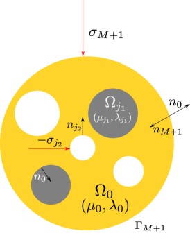
Figure 1: Geometry setting of the model where $j_{1}\in J_{1}$ and $j_{2}\in J_{2}$.

In the numerical example presented below, we assume that each inclusion $\Omega_{i}$, $i\in J_{1}$ is filled with an isotropic elastic medium associated with Lamé parameters $\mu_{i},\lambda_{i}$. The remaining background domain $\Omega_{0}$ is filled with medium of Lamé constants $\mu_{0},\lambda_{0}$. Further, we denote ${\mathcal{T}^{i}_{{\bf n}_{j}}}^{\pm}$ the normal derivative operator acting on the boundary $\Gamma_{j}$ with Lamé constants $\mu_{j},\lambda_{j}$ and the normal vector ${\bf n}_{j}$:

$${\mathcal{T}^{i}_{{\bf n}_{j}}}^{\pm}u=\gamma_{j}^{\pm}\Big{(}(2\mu_{i}e(u)+\lambda_{i}\mathop{\rm Tr}e(u)\mathop{\rm Id}){\bf n}_{j}\Big{)}$$

where $\gamma^{\pm}_{j}$ are the exterior and interior the trace operators on $\Gamma_{j}$, following the notations given by (2.4) by taking $\Omega^{-}=\Omega_{j}$. Define the parameter $s_{i}$ by

$$s_{i}=\begin{cases}-1&i=M+1,\\ 1&\mbox{else}.\end{cases}$$ (6.3)

In particular, write

$$\llbracket\mathcal{T}u\rrbracket={\mathcal{T}^{0}_{s_{i}{\bf n}_{i}}}^{-}u-{\mathcal{T}^{0}_{s_{i}{\bf n}_{i}}}^{+}u,\qquad\mbox{on}~{}\Gamma_{i},~{}i\in J_{1}\cup J_{2}$$ (6.4)

and it is obvious that

$${\mathcal{T}^{0}_{s_{i}{\bf n}_{i}}}^{\pm}=s_{i}{\mathcal{T}^{0}_{{\bf n}_{i}}}^{\pm}.$$

For given $f_{i}\in H^{-\frac{1}{2}}(\Gamma_{i})^{3}$, we impose the transmission condition:

$$\llbracket u\rrbracket=0,\qquad\llbracket\mathcal{T}u\rrbracket=f_{i},\qquad\mbox{on}~{}\Gamma_{i},i\in J_{1}.$$

Further, we let the domain $\Omega$ be subjected of a given stress tensor on its boundary. Indeed, we let each part of the boundary $\Gamma_{i}$, $i\in J_{2}$ be subjected to a given stress tensor $\sigma_{i}\in H^{1/2}(\Gamma_{i})^{3}$:

$${\mathcal{T}^{0}_{{\bf n}_{i}}}^{+}u=-s_{i}\sigma_{i}.$$ (6.5)

Then, we consider the solution $u\in V_{0}(\Omega)^{3}$ to the following interface problem:

$$\begin{array}[]{rlll}-\mathop{\rm div}\big{(}2\mu_{i}e(u)+\lambda_{i}\mathop{\rm Tr}e(u)\mathop{\rm Id}\big{)}&=0,&\mbox{in }\Omega_{i},~{}i\in\{0\}\cup J_{1},\\ \llbracket u\rrbracket&=0,&\mbox{on }\Gamma_{i}~{}i\in J_{1},\\ \llbracket\mathcal{T}u\rrbracket&=f_{i},&\mbox{on }\Gamma_{i}~{}i\in J_{1},\\ {\mathcal{T}^{0}_{{\bf n}_{i}}}^{+}u&=-s_{i}\sigma_{i},&\mbox{on }\Gamma_{i},i\in J_{2}.\end{array}$$ (6.6)

Standard arguments involving the Lax-Milgram theorem yields the well-posedness of the problem.

Remark 6.1.

In our case, we pre-defined the index set $J_{2}$ with the condition $M+1\in J_{2}$. However, by equipping the domain $\Omega_{M+1}$ (which is indeed the exterior domain of the sphere $B_{R}$) with Lamé parameters $\mu_{M+1},\lambda_{M+1}$, one can also relax the setting and consider the case where $M+1\in J_{1}$.

6.2 Integral equation

Let $u\in V_{0}(\Omega)^{3}$ denote the solution to (6.6) satisfying $\llbracket u\rrbracket=0$ on $\Gamma_{i}$ for $i\in J_{1}$ and define $\nu$ on $\Gamma_{0}$ by

$$\nu=\gamma_{0}^{-}u\qquad\mbox{as well as}\qquad\quad\nu_{i}=\nu|_{\Gamma_{i}},\quad\forall i\in J_{1}\cup J_{2},$$

where $\gamma_{0}^{-}$ is the trace operator $\gamma_{0}^{-}\colon H^{1}(\Omega_{0})^{3}\rightarrow H^{\frac{1}{2}}(\Gamma_{0})^{3}$ defined by (2.4) for $\Omega^{-}=\Omega_{0}$. To deduce an integral equation for $\nu$, we first introduce an auxiliary problem: find a solution $v\in H^{1}(\Omega)^{3}$ to

$$\begin{array}[]{rll}-\mathop{\rm div}\big{(}2\mu_{0}e(v)+\lambda_{0}\mathop{\rm Tr}e(v)\mathop{\rm Id}\big{)}&=0,{}&\mbox{in }\Omega\textbackslash\Gamma_{0},\\ \gamma_{0}^{-}v&=\gamma_{0}^{-}u,{}&\mbox{on }\Gamma_{0}.\end{array}$$ (6.7)

The auxiliary problem (6.7) admits a unique solution $v$ in $\Omega$ and observe that

$$v=u,\quad~{}\mbox{in}~{}\Omega_{0},$$

but is different in all $\Omega_{i}$, $i\in J_{1}$. Further, there exists a global density $\phi$ supported on $\Gamma_{0}$ such that

$$\begin{array}[]{ll}v=\mathcal{S}_{G}^{0}\phi=\sum\limits_{i\in J_{1}\cup J_{2}}\mathcal{S}^{0}_{i}\phi_{i}&\text{in}~{}\Omega_{0}\\ v=\mathcal{V}_{G}^{0}\phi=\sum\limits_{i\in J_{1}\cup J_{2}}\mathcal{V}^{0}_{i}\phi_{i}&\mbox{on}~{}\Gamma_{0},\end{array}$$ (6.8)

where $\mathcal{S}_{G}^{0}$ is the global layer potential (3.1) with Lamé parameters $\mu_{0},\lambda_{0}$ defined on the whole boundary $\Gamma_{0}$ while $\mathcal{S}_{i}^{0}$ is the local single layer potential with Lamé parameters $\mu_{0},\lambda_{0}$ defined locally on the sphere $\Gamma_{i}$ and $\mathcal{V}_{G}^{0},\mathcal{V}^{0}_{i}$ their corresponding single layer boundary operators (3.2). Further, according to Theorem 3.4, the density $\phi_{i}$ is given by the jump relation

$$\phi_{i}=\llbracket\mathcal{T}v\rrbracket=\Big{(}{\mathcal{T}_{s_{i}{\bf n}_{i}}^{0}}^{-}v-{\mathcal{T}_{s_{i}{\bf n}_{i}}^{0}}^{+}v\Big{)}=s_{i}\Big{(}{\mathcal{T}_{{\bf n}_{i}}^{0}}^{-}u-{\mathcal{T}_{{\bf n}_{i}}^{0}}^{+}v\Big{)},\quad~{}\mbox{on}~{}\Gamma_{i},i\in J_{1}\cup J_{2}.$$ (6.9)

The last equivalence in (6.9) is obtained because $u=v$ on $\Omega_{0}$. Further, both solutions $u,v$ can be represented by some local densities in each domain $\Omega_{i}$:

$$\begin{array}[]{ll}u|_{\Omega_{i}}=\mathcal{S}_{i}\varphi_{i},&i\in J_{1}\\ v|_{\Omega_{i}}=\mathcal{S}_{i}^{0}\psi_{i}&i\in J_{1}\cup J_{2},\end{array}$$

where $\mathcal{S}_{i}$ is the local layer potential with Lamé parameters $\mu_{i},\lambda_{i}$ while $\mathcal{S}_{i}^{0}$ with $\mu_{0},\lambda_{0}$, both of which are defined locally on the sphere $\Gamma_{i}$. For the corresponding single layer boundary operators $\mathcal{V}_{i}^{0},\mathcal{V}_{i}$ defined by (3.2), we have

$$\mathcal{V}_{i}^{0}\psi_{i}=\mathcal{V}_{i}\varphi_{i}=\nu_{i},\quad i\in J_{1}.$$

According to Corollary 3.6, the single layer boundary operators $\mathcal{V}_{i}^{0},\mathcal{V}_{i}$ are invertible, so we have

$$\begin{array}[]{ll}\psi_{i}={\mathcal{V}_{i}^{0}}^{-1}(\gamma_{i}v)={\mathcal{V}_{i}^{0}}^{-1}\nu_{i},&\mbox{on }~{}\Gamma_{i},i\in J_{1}\cup J_{2},\\ \varphi_{i}=\mathcal{V}_{i}^{-1}(\gamma_{i}u)=\mathcal{V}_{i}^{-1}\nu_{i},&\mbox{on }~{}\Gamma_{i},i\in J_{1}.\end{array}$$ (6.10)

Now, according to Theorem 3.3, we have

$$\begin{array}[]{ll}{\mathcal{T}_{{\bf n}_{i}}^{0}}^{-}\mathcal{S}_{i}^{0}\psi_{i}=s_{i}{1\over 2}\psi_{i}+{\mathcal{K}_{i}^{0}}^{*}\psi_{i},&\mbox{on }~{}\Gamma_{i},i\in J_{1}\cup J_{2},\\ {\mathcal{T}_{{\bf n}_{i}}^{i}}^{-}\mathcal{S}_{i}\varphi_{i}=s_{i}{1\over 2}\varphi_{i}+\mathcal{\mathcal{K}}^{*}_{i}\varphi_{i},&\mbox{on }~{}\Gamma_{i},i\in J_{1},\\ \end{array}$$ (6.11)

where ${\mathcal{K}_{i}^{0}}^{*}$, $\mathcal{K}_{i}^{*}$ are adjoint double layer boundary operators (3.5) defined locally on $\Gamma_{i}$ with Lamé constants $\mu_{0},\lambda_{0}$ and $\mu_{i},\lambda_{i}$ respectively. In problem (6.6), we have

$${\mathcal{T}_{{\bf n}_{i}}^{0}}^{+}u=\begin{cases}{\mathcal{T}_{{\bf n}_{i}}^{i}}^{-}\mathcal{S}_{i}\varphi_{i}-f_{i},&\mbox{on }~{}\Gamma_{i},i\in J_{1},\\ -s_{i}\sigma_{i},&\mbox{on }~{}\Gamma_{i},i\in J_{2},\end{cases}$$

where $f_{i}\in H^{-\frac{1}{2}}(\Gamma_{i})^{3},\sigma_{i}\in H^{\frac{1}{2}}(\Gamma_{i})^{3}$ are given transmission conditions and Neuman boundary conditions respectively. Providing (6.9)–(6.11), we have

$$\phi_{i}=\begin{cases}{1\over 2}({\mathcal{V}_{i}^{0}}^{-1}-\mathcal{V}_{i}^{-1})\nu_{i}+({\mathcal{K}_{i}^{0}}^{*}{\mathcal{V}_{i}^{0}}^{-1}-{\mathcal{K}_{i}}^{*}\mathcal{V}_{i}^{-1})\nu_{i}+f_{i},&i\in J_{1},\\ {1\over 2}{\mathcal{V}_{i}^{0}}^{-1}\nu_{i}+s_{i}{\mathcal{K}_{i}^{0}}^{*}{\mathcal{V}_{i}^{0}}^{-1}\nu_{i}+s_{i}\sigma_{i},&i\in J_{2}.\end{cases}$$

According to (6.8), we have

$$(\mathop{\rm Id}-\mathcal{V}_{G}^{0}\mathcal{L})\nu=\mathcal{V}_{G}^{0}\Sigma$$ (6.12)

where $\mathcal{L}$ is an operator defined on each $\Gamma_{i}$:

$$\mathcal{L}|_{\Gamma_{i}} =\mathcal{L}_{i}={1\over 2}({\mathcal{V}_{i}^{0}}^{-1}-\mathcal{V}_{i}^{-1})+({\mathcal{K}_{i}^{0}}^{*}{\mathcal{V}_{i}^{0}}^{-1}-{\mathcal{K}_{i}}^{*}\mathcal{V}_{i}^{-1}), i\in J_{1},$$

$$\mathcal{L}|_{\Gamma_{i}} =\mathcal{L}_{i}={1\over 2}{\mathcal{V}_{i}^{0}}^{-1}\nu_{i}+s_{i}{\mathcal{K}_{i}^{0}}^{*}{\mathcal{V}_{i}^{0}}^{-1}\nu_{i}, i\in J_{2},$$

and the vector $\Sigma$ satisfies

$$\Sigma|_{\Gamma_{i}}=\begin{cases}f_{i},&i\in J_{1},\\ \sigma_{i},&i\in J_{2}.\end{cases}$$

6.3 Galerkin approximation

Introduce $V_{N,i},i\in J_{1}\cup J_{2}$ the set spanned by vector spherical harmonics (4.4) on the sphere $\Gamma_{i}$ with a maximum degree $N$:

$$V_{N,i}=\Big{\{}\sum\limits_{\ell=0}^{N}\sum\limits_{m=-\ell}^{\ell}\sum\limits_{k=1}^{3}[y_{i}]_{\ell m}^{k}Y_{\ell m}^{ki}(x)\Big{|}[y_{i}]_{\ell m}^{k}\in\mathbb{R}\Big{\}},$$ (6.13)

where we write $Y_{\ell m}^{1}=V_{\ell m},Y_{\ell m}^{2}=W_{\ell m},Y_{\ell m}^{3}=X_{\ell m}$ and $Y_{\ell m}^{ki}(x)=Y_{\ell m}^{k}\left({x-x_{i}\over r_{i}}\right).$ Define also the global set

$$V_{N}=\bigotimes\limits_{i\in J_{1}\cup J_{2}}V_{N,i}.$$ (6.14)

We look for the approximation of $\nu_{N}\in V_{N}$ to (6.6) with

$$\forall i\in J_{1}\cup J_{2},\forall v_{N,i}\in V_{N,i}:\quad\langle\nu_{N,i}-\mathcal{V}^{0}_{G}\mathcal{L}\nu_{N},v_{N,i}\rangle_{\Gamma_{i}}=\langle\mathcal{V}^{0}_{G}\Sigma,v_{N,i}\rangle_{\Gamma_{i}}.$$ (6.15)

In practice, we use the quadrature (4.7) to approximate the inner product and the approximate solution $\nu_{N}$ on each $\Gamma_{i}$ thus satisfies

$$\forall i\in J_{1}\cup J_{2},\forall v_{N,i}\in V_{N,i}:\quad\langle\nu_{N,i}-\mathcal{V}^{0}_{G}\mathcal{L}\nu_{N},v_{N,i}\rangle_{\Gamma_{i},t}=\langle\mathcal{V}^{0}_{G}\Sigma,v_{N,i}\rangle_{\Gamma_{i},t}.$$

Denote by $\mathcal{M}=3(N+1)^{2}(|J_{1}|+|J_{2}|)$ the number of degrees of freedom. The $\mathbb{R}^{\mathcal{M}}$-vector collecting all the coefficients $[y]_{\ell m}^{k}$ denoted by ${\bf\Lambda}$ yields the linear system

$$({\bf D}-{\bf N}){\bf\Lambda}={\bf F},$$ (6.16)

where by (4.5), (4.6), the $\mathcal{M}\times\mathcal{M}$ diagonal matrix ${\bf D}$ is given by

$$[D_{ii}]_{\ell m,\ell m}^{11}=(2\ell+1)(\ell+1),\qquad[D_{ii}]_{\ell m,\ell m}^{22}=(2\ell+1)\ell,\qquad[D_{ii}]_{\ell m,\ell m}^{33}=(\ell+1)\ell,$$

and where $\bf{N}$ is a $\mathcal{M}\times\mathcal{M}$ matrix with coefficients

$$[N_{ij}]_{\ell m,l^{\prime}m^{\prime}}^{kk^{\prime}}=\big{\langle}\mathcal{V}_{G}^{0}\mathcal{L}_{j}Y_{\ell^{\prime}m^{\prime}}^{k^{\prime}},Y_{\ell m}^{ki}\big{\rangle}_{\Gamma_{i},t}.$$ (6.17)

The right hand side ${\bf F}\in\mathbb{R}^{\mathcal{M}}$ is given by its coefficients:

$$[F_{i}]_{\ell m}^{k}=\langle\mathcal{V}_{G}^{0}\Sigma,Y_{\ell m}^{ki}\rangle_{\Gamma_{i},t}.$$ (6.18)

To derive the entries of the matrix (6.17), recall the spectral results in Lemma 5.1 so that we have on $\Gamma_{j}$

$${\mathcal{V}_{j}}^{-1}Y_{\ell^{\prime}m^{\prime}}^{k^{\prime}j} ={1\over r_{j}\tau^{k^{\prime}j}_{\mathcal{V},\ell^{\prime}}}Y_{\ell^{\prime}m^{\prime}}^{k^{\prime}j}, {\mathcal{V}_{j}^{0}}^{-1}Y_{\ell^{\prime}m^{\prime}}^{k^{\prime}j} ={1\over r_{j}\tau^{k^{\prime}0}_{\mathcal{V},\ell^{\prime}}}Y_{\ell^{\prime}m^{\prime}}^{k^{\prime}j},$$

$$\mathcal{K}^{*}_{j}Y_{\ell^{\prime}m^{\prime}}^{k^{\prime}j} =\tau^{k^{\prime}j}_{\mathcal{K}^{*},\ell^{\prime}}Y_{\ell^{\prime}m^{\prime}}^{k^{\prime}j}, \mathcal{K}^{*0}_{j}Y_{\ell^{\prime}m^{\prime}}^{k^{\prime}j} =\tau^{k^{\prime}0}_{\mathcal{K}^{*},\ell^{\prime}}Y_{\ell^{\prime}m^{\prime}}^{k^{\prime}j},$$

where $\tau^{k^{\prime}j}_{\mathcal{V},\ell^{\prime}},\tau^{k^{\prime}j}_{\mathcal{K}^{*},\ell^{\prime}}$ are eigenvalues of the single and double layer boundary operator with Lamé constants $\mu_{j},\lambda_{j}$ given by (5.2), (5.5) respectively. Hence, we have

$$\mathcal{L}_{j}Y_{\ell^{\prime}m^{\prime}}^{k^{\prime}j}={1\over r_{j}}C_{j\ell^{\prime}k^{\prime}}Y_{\ell^{\prime}m^{\prime}}^{k^{\prime}j},$$

where the constant $C_{j\ell^{\prime}k^{\prime}}$ reads

$$C_{j\ell^{\prime}k^{\prime}}=\begin{cases}{1\over 2}\Big{(}{1\over\tau^{k^{\prime}0}_{\mathcal{K}^{*},\ell^{\prime}}}-{1\over\tau^{k^{\prime}j}_{\mathcal{V},l^{\prime}}}\Big{)}+\Big{(}{\tau^{k^{\prime}0}_{\mathcal{K}^{*},\ell^{\prime}}\over\tau^{k^{\prime}0}_{\mathcal{V},\ell^{\prime}}}-{\tau^{k^{\prime}j}_{\mathcal{K}^{*},\ell^{\prime}}\over\tau^{k^{\prime}j}_{\mathcal{V},\ell^{\prime}}}\Big{)}&j\in J_{1},\\ {1/2+s_{i}\tau^{k^{\prime}0}_{\mathcal{K}^{*},\ell^{\prime}}\over\tau^{k^{\prime}0}_{\mathcal{V},\ell^{\prime}}}&j\in J_{2}.\end{cases}$$

Recall that $s_{i}$ denotes the parameter defined by (6.3). Further, by (5.3), (5.4),

$$(\mathcal{S}_{j}^{0}Y_{\ell^{\prime}m^{\prime}}^{k^{\prime}})(x)=\begin{cases}r_{j}\Big{[}\underline{Y_{\ell^{\prime}m^{\prime}}}\Big{(}{x-x_{j}\over|x-x_{j}|}\Big{)}A_{\mathcal{V},\ell^{\prime}}^{in}\Big{(}{x-x_{j}\over r_{j}}\Big{)}\Big{]}_{k^{\prime}}&|x-x_{j}|\leq r_{j},\\ r_{j}\Big{[}\underline{Y_{\ell^{\prime}m^{\prime}}}\Big{(}{x-x_{j}\over|x-x_{j}|}\Big{)}A_{\mathcal{V},\ell^{\prime}}^{out}\Big{(}{x-x_{j}\over r_{j}}\Big{)}\Big{]}_{k^{\prime}}&|x-x_{j}|>r_{j},\end{cases}$$

where $[\cdot]_{k^{\prime}}$ denotes the $k^{\prime}$-th column of the obtained matrix. Hence, the coefficient $[N_{ij}]_{\ell m,\ell^{\prime}m^{\prime}}^{kk^{\prime}}$ of the matrix ${\bf N}$ (6.17) reads

$$[N_{ij}]_{\ell m,\ell^{\prime}m^{\prime}}^{kk^{\prime}}=\langle\mathcal{V}_{G}^{0}\mathcal{L}_{j}Y_{\ell^{\prime}m^{\prime}}^{k^{\prime}},Y_{\ell m}^{ki}\rangle_{\Gamma_{i},t}$$

$$=C_{j\ell^{\prime}k^{\prime}}\sum\limits_{t=1}^{T_{g}}w_{t}Y_{\ell m}^{ki}(s_{t})\mathcal{S}_{j}^{0}Y_{\ell^{\prime}m^{\prime}}^{k^{\prime}}(x_{i}+r_{i}s_{t})=C_{j\ell^{\prime}k^{\prime}}\sum\limits_{t=1}^{T_{g}}w_{t}Y_{\ell m}^{ki}(s_{t})\Big{[}\underline{Y_{\ell^{\prime}m^{\prime}}}\Big{(}{y_{ij}^{t}\over|y_{ij}^{t}|}\Big{)}A_{\mathcal{V},\ell^{\prime}}^{f(j)}\Big{(}{y_{ij}^{t}\over r_{j}}\Big{)}\Big{]}_{k^{\prime}},$$

where $y_{ij}^{t}=x_{i}+r_{i}s_{t}-x_{j}$ and $f(j)$ takes the value

$$f(j)=\begin{cases}in&j=M+1,\\ out&else.\end{cases}$$

In particular, when $i=j$, we use (4.5) for the exact value of the inner product and obtain:

$$[N_{ii}]_{\ell m,\ell^{\prime}m^{\prime}}^{kk^{\prime}}=\sum\limits_{l^{\prime}=0}^{N}\sum\limits_{m^{\prime}=-\ell^{\prime}}^{\ell^{\prime}}C_{i\ell^{\prime}k^{\prime}}\tau_{\mathcal{V},\ell}^{k^{\prime},0}\langle Y_{\ell m}^{ki},Y_{\ell^{\prime}m^{\prime}}^{k^{\prime}i}\rangle_{\Gamma_{i}}.$$

Finally, the right-hand side vector ${\bf F}$ with coefficient $[F_{i}]_{\ell m}^{k}$ is given by:

$${[F_{i}]}_{\ell m}^{k}= \sum\limits_{\ell^{\prime}=0}^{N}\sum\limits_{m^{\prime}=-\ell^{\prime}}^{\ell^{\prime}}\sum\limits_{k^{\prime}=1}^{3}\Bigg{(}r_{i}[\Sigma_{i}]_{\ell^{\prime}m^{\prime}}^{k^{\prime}}\tau^{k^{\prime}0}_{\mathcal{V},\ell^{\prime}}\langle Y_{\ell^{\prime}m^{\prime}}^{k^{\prime}i},Y_{\ell m}^{ki}\rangle_{\Gamma_{i}}$$

$$+\sum\limits_{\mathclap{\begin{subarray}{c}j\in J_{1}\cup J_{2}\\ j\neq i\end{subarray}}}r_{j}\sum\limits_{t=1}^{T_{g}}[\Sigma_{j}]_{\ell^{\prime}m^{\prime}}^{k^{\prime}}w_{t}Y_{\ell m}^{ki}(s_{t})\Big{[}\underline{Y_{\ell^{\prime}m^{\prime}}}\Big{(}{y_{ij}^{t}\over|y_{ij}^{t}|}\Big{)}A_{\mathcal{V},\ell^{\prime}}^{f(j)}\Big{(}{y_{ij}^{t}\over r_{j}}\Big{)}\Big{]}_{k^{\prime}}\Bigg{)},~{}i\in J_{1}\cup J_{2}$$

where $[\Sigma_{i}]_{\ell m}^{k}\in\mathbb{R}$ is determined by the right-hand side vector $\Sigma$ in (6.12) :

$$\Sigma|_{\Gamma_{i}}=\sum\limits_{\ell=0}^{N}\sum\limits_{m=-\ell}^{\ell}\sum\limits_{k=1}^{3}[\Sigma_{i}]_{\ell m}^{k}Y_{\ell m}^{ki}(x).$$

Remark 6.2.

A similar physical model called “Finite Cluster Model” was considered in [22] in where an algebraic formulation is derived through the use of M2L-operators (using the fast multipole method terminology). However, with the jump relations given in (3.10), the algebraic formulation of the “Finite Cluster Model” can be proven to be equivalent to the discrete integral formulation (6.15) presented above.

It shall be noted that the mathematical framework introduced here through the use of layer potentials and boundary operators in order to derive an integral equation (6.12) defining the exact solution and and the subsequent introduction of the Galerkin discretization (6.15) allows a mathematical analysis which will be subject of an upcoming work.

7 Numerical tests

For all following computations, we chose the number of Lebedev integration points $T_{g}$ such that, for given $N$, products of two scalar spherical harmonics of maximal degree $N$, thus spherical harmonics of degree $2N$, are integrated exactly. The number of points can then be extracted from Table 1.

7.1 One sphere model

We start with a simple model involving only one single sphere whose solution can be computed analytically in order to assess the convergence of the method in this simple setting. For simplicity, let $\mathbb{S}^{2}\subset\mathbb{R}^{3}$ be the unit sphere on which a stress tensor $\sigma\in H^{\frac{1}{2}}(\mathbb{S}^{2})^{3}$ is imposed and let the Lamé constants be $\mu_{0}=\lambda_{0}=1$. Let ${\bf n}$ be the outward pointing normal vector with respect to the unit sphere $\mathbb{S}^{2}$. The solution $u\in V_{0}(B)^{3}$ to the problem

$$\begin{array}[]{r}-\mathop{\rm div}\big{(}2e(u)+\mathop{\rm Tr}e(u)\mathop{\rm Id}\big{)}=0,\quad\mbox{in }B,\\ {\mathcal{T}_{\bf n}}^{-}u=\sigma\quad\mbox{on }\mathbb{S}^{2},\end{array}$$

reads

$$u(x)=\big{(}\mathcal{S}(1+\mathcal{K}^{*})^{-1}\sigma\big{)}(x),\quad\forall x\in\mathbb{R}^{3},$$ (7.1)

with $\mathcal{S}$ being the single layer potential (3.1) and $\mathcal{K}^{*}$ the adjoint of the double layer boundary operator (3.5). For the given tensor $\sigma$, if there exists an integer $\ell_{\mathop{\rm ex}}$ such that we can expand $\sigma$ by means of vector spherical harmonics up to order $\ell_{\mathop{\rm ex}}$:

$$\sigma(x)=\sum\limits_{\ell=1}^{\ell_{\mathop{\rm ex}}}\sum\limits_{m=-\ell}^{\ell}\sum\limits_{k=1}^{3}[\Sigma]_{\ell m}^{k}Y_{\ell m}^{k}(x),$$

then the exact solution restricted to the sphere $\Lambda_{\mathop{\rm ex}}=u|_{\mathbb{S}^{2}}$ is given explicitly by

$$\Lambda_{\mathop{\rm ex}}=\sum\limits_{\ell=1}^{\ell_{\mathop{\rm ex}}}\sum\limits_{m=-\ell}^{\ell}\sum\limits_{k=1}^{3}{\tau_{\mathcal{V},\ell}^{k}\over{1\over 2}+\tau_{\mathcal{K}^{*},\ell}^{k}}[\Sigma]_{\ell m}^{k}Y_{\ell m}^{k}(x),$$ (7.2)

where $\tau_{\mathcal{V},\ell}^{k},\tau_{\mathcal{K}^{*},\ell}^{k}$ are the eigenvalues of the single layer boundary operator and the adjoint double layer boundary operator given by (5.2) and (5.5) resp. They only concern in computing (7.2) is that the denominator tends to zero if $\tau_{\mathcal{K}^{*},\ell}^{k}$ approaches $-1/2$. Recall that according to Remark 5.3, the only possible eigenvectors of $\mathcal{K}^{*}$ with the eigenvalue $-1/2$ are $W_{1,-1},W_{1,0},W_{1,1}$. According to Appendix A, we see that they are constant and parallel to the cartesian basis ${\bf e}_{i},i=1,2,3$. To ensure that (7.2) is well defined and these modes avoided, we simply impose that

$$\int_{\mathbb{S}^{2}}\sigma=0.$$

We consider the following four cases:

• Case 1. $\sigma=-(x,y,z)^{\top}$.

• Case 2. $\sigma=-(x,0,0)^{\top}$.

• Case 3. $\sigma=-(x^{7},y^{7},z^{7})^{\top}$.

• Case 4. $\sigma=-\big{(}\sin(2\pi x),\sin(2\pi y),\sin(2\pi z)\big{)}^{\top}$.

Table 2 lists the $L^{2}$ norm of the numerical solution on the unit sphere $||\Lambda_{s}||_{L^{2}}$ in each case with different degrees of vector spherical harmonics and the relative error is defined by

$${\tt Re}={||\Lambda_{s}-\Lambda_{{\rm ex}}||_{L^{2}}\over||\Lambda_{{\rm ex}}||_{L^{2}}}.$$ (7.3)

The exact solutions $\Lambda_{{\rm ex}}$ in the first three cases are exactly computed by the (7.1), (7.2) while the in the last cases, the “exact” solution is obtained by taking a large enough $\ell_{\mathop{\rm ex}}$ (in this case $\ell_{\mathop{\rm ex}}$ = 50).

$N$	Case 1		Case 2		Case 3		Case 4
2	0		0		1.985e-01		5.375e-01
5	0		0		4.020e-03		6.797e-02
8	0		0		4.796e-09		1.370e-04
11	0		0		0		7.892e-13
14	0		0		0		7.097e-13

Table 2: Relative error ${\tt Re}$ of the approximation to the one-sphere model.

7.2 Convergence with respect to the degree $N$

We study now the convergence of the error measured in the $L^{2}$ norm with respect to the degree $N$ of the vector spherical harmonics. Using the notation introduced in Section 6, we test a model with $M=2$ and

$$J_{1}=\{1\},\quad J_{2}=\{2,3\}.$$

Let $\Gamma_{1}$ be the sphere centered at $(1,0,0)$ respectively with radius $0.1$ and $\Gamma_{2}$ centered at $(-1,0,0)$ with radius $0.1$ while $\Gamma_{3}$ is centered at $(0,0,0)$ with radius $2$. The inclusion $\Omega_{1}$ is filled with a medium represented by the Lamé constants $\mu_{1}=10,\lambda_{1}=10$ while the background domain $\Omega_{0}$ uses $\mu_{0}=1,\lambda_{0}=1$ as Lamé parameters.

The interface condition $\llbracket\mathcal{T}u\rrbracket=0$ is imposed on $\Gamma_{1}$ while the spheres $\Gamma_{2},\Gamma_{3}$ are subjected to a stress tensor $\mathcal{T}_{{\bf n}_{2}}^{+}u=-\sigma_{2}$ respectively $\mathcal{T}_{{\bf n}_{3}}^{+}u=\sigma_{3}$. Table 3 illustrates the parameters of the above geometry configuration.

Set	Sphere	Center	Radius	Lamé constants	Stress tensor	Transmission
$J_{1}$	$\Gamma_{1}$	$(1,0,0)$	0.1	$\mu_{1}=10,\lambda_{1}=10$	———	$\llbracket\mathcal{T}u\rrbracket=0$
$J_{2}$	$\Gamma_{2}$	$(-1,0,0)$	0.1	———	$\mathcal{T}_{{\bf n}_{2}}^{+}u=-\sigma_{2}$	———
$J_{2}$	$\Gamma_{3}$	$(0,0,0)$	2	$\mu_{0}=1,\lambda_{0}=1$	$\mathcal{T}_{{\bf n}_{3}}^{+}u=\sigma_{3}$	———

Table 3: Geometric configuration of the case study for convergence with respect to the degree of vector spherical harmonics $N$ involving three spheres.

We now test two cases to see the relation between the relative error and the degree of the spherical harmonics for different kinds of imposed stress tensors $\sigma_{2},\sigma_{3}$:

1. The two stress tensors are set to be smooth functions such that

   $$\begin{array}[]{l}\mathcal{T}_{{\bf n}_{2}}^{+}u=-\sigma_{2}=10\big{(}\sin(2\pi(x+1)),\sin(2\pi(y+1)),\sin(2\pi(z+1))\big{)}^{\top},\\ \mathcal{T}_{{\bf n}_{3}}^{+}u=\sigma_{3}=-2\big{(}\sin(2\pi x),\sin(2\pi y),\sin(2\pi z)\big{)}^{\top}.\end{array}$$ (7.4)

2. The stress tensors are set to be piecewise smooth such that

   $$\mathcal{T}_{{\bf n}_{2}}^{+}u=-\sigma_{2}=\begin{cases}(0.2,0,0)^{\top}&x\geq 0,\\ -(0.2,0,0)^{\top}&x<0,\end{cases}$$ (7.5)

   and

   $$\mathcal{T}_{{\bf n}_{3}}^{+}u=\sigma_{3}=\begin{cases}(1,0,0)^{\top}&x\geq 0,\\ -(1,0,0)^{\top}&x<0.\end{cases}$$ (7.6)

We compute the “exact” solution to the problem with a large degree of vector spherical harmonics ($N_{\rm ex}=50$) for both cases. In the Figure 2, we illustrate the log of the relative error (7.3) with respect to the degree $N$ of spherical harmonics of the two tests above. We observe exponential convergence in the first case where the given stress tensor is regular. In the second case, the situation is less clear as an initial pre-asymptotic is followed by a very fast convergence and the asymptotic regime is not yet reached, but the absolute error is already very small.

Figure 2: The $L^{2}$ error of the approximation with respect to the degree of spherical harmonics for the test cases (7.4) (left) and (7.5)–(7.6) (right).

7.3 Computational cost

Next, we study the computational cost of our numerical method by considering an “embedded model” with $M$ inclusions by increasing the value of $M$. We do the following test with Matlab on an iMac with a 2,7 GHz Intel Core i5 processor.

We consider a case where a stress tensor ${\mathcal{T}^{0}{{\bf n}_{M+1}}}^{+}u=-{1\over R}(x,y,z)^{\top}$ is imposed on a origin-centered sphere with radius $R$, denoted by $\mathbb{S}^{2}_{R}$. Inclusions are taken to be all the spheres with radii $0.1$, centered on a cubic lattice $\mathbb{Z}^{3}$ and which are contained in $\mathbb{S}^{2}_{R}$. We increase the number of inclusions $M$ by increasing the value of the radius $R$ of the big sphere. Table 4 lists the number of spheres with respect to the radius $R$ that grows of course cubically.

Radius of the big sphere	1	2	3	4	5
Number of total spheres	2	28	94	252	486

Table 4: Number of spheres w.r.t the radius $R$

We fill each small inclusion with a medium associated with the Lamé constants $\mu_{i}=10,\lambda_{i}=10$, $i=1,...,M$ and take the transmission condition $\llbracket\mathcal{T}u\rrbracket=0$ on each embedded sphere. Further, the Lamé constants of the background domain are fixed to be $\mu_{0}=1,\lambda_{0}=1$. The degree of the vector spherical harmonics is chosen to be $N=3$. Further, we stop the iterative solver of the linear system when the residual is smaller than $10^{-6}$. Figure 3 illustrates the computed elastic deformation of the model computed when $R=3$. The colorcode represents the modulus of the displacement.

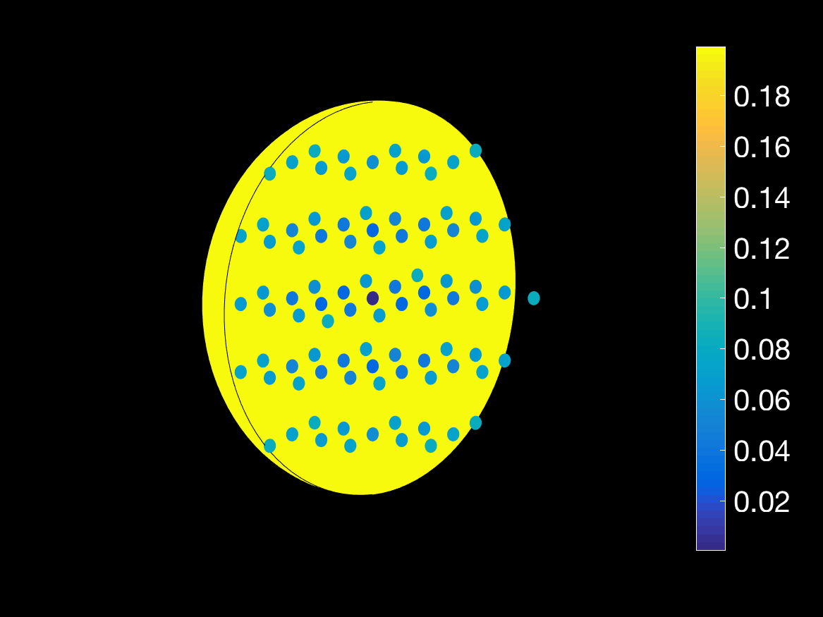
Figure 3: The elastic deformation of the embedded model when $R=3$. The colorcode represents the modulus of the displacement.

We report the result of the computational time in Figure 4 which illustrates that the computational cost with respect to the number of spheres grows as $O(M^{2})$. This is the normal scaling for an integral equation involving $M$ spheres, whose iterative solver requires a number of iterations that is independent of $M$ which we observe.

Figure 4: The run time in second with respect to the number $M$ of spheres (log-log scale).

7.4 The effect of an inclusion

We now consider the unit ball $B_{1}$ which contains an additional inclusion $\Omega_{1}$ in form of a sphere centered at the origin with radius $0.5$. We study how the displacement on the unit sphere $\mathbb{S}^{2}$ is influenced by the compressibility of the small inclusions $\Omega_{1}$. We will use the Poisson’s ratio as the parameter defined by (1.2) describing the compressibility of a substance.

Let the stress tensor $-(x,y,z)^{\top}$ be imposed on the unit sphere $\mathbb{S}^{2}$ and fix the shear modulus of the exterior shell $\Omega_{0}=B_{1}\backslash\overline{\Omega}_{1}$ to be $\mu_{0}=1$ and the shear modulus $\mu_{1}=1$ for the inclusion $\Omega_{1}$. We test several cases where the the exterior shell and the inclusion are associated to different Poisson’s ratio $\nu_{0},\nu_{1}$. Recall that $\nu_{0},\nu_{1}\in(-1,1/2)$ according to the definition, we have the limit values of the first Lamé parameter $\lambda_{1}$:

$$\lambda_{1}\xrightarrow[\nu_{1}\to-1]{}-{2\over 3},\quad\lambda_{1}\xrightarrow[\nu_{1}\to{1\over 2}]{}\infty.$$

In Figure 5, we plot the $L^{2}$ norm of the displacement on the unit sphere by letting the Poisson’s ratio $\nu_{1}$ vary in $[-1,0.4998]$ with different given values of Poisson’s ratio $\nu_{0}$ of the background domain $\Omega_{0}$. In Figure 6, we give two solutions with different Poisson’s ratios: the left solution is obtained by setting $\nu_{1}=0.4995$ while the other is obtained by setting $\nu=-1$, both embedded into a background domain with $\nu_{0}=1/6$.

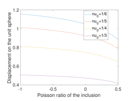
Figure 5: The $L^{2}$ norm of the solution on the unit sphere with respect to the Poisson’s ratio $\nu_{1}$ of the inclusion. Each curve is obtained by a given background Poisson’s ratio $\nu_{0}$ specified by the legend.

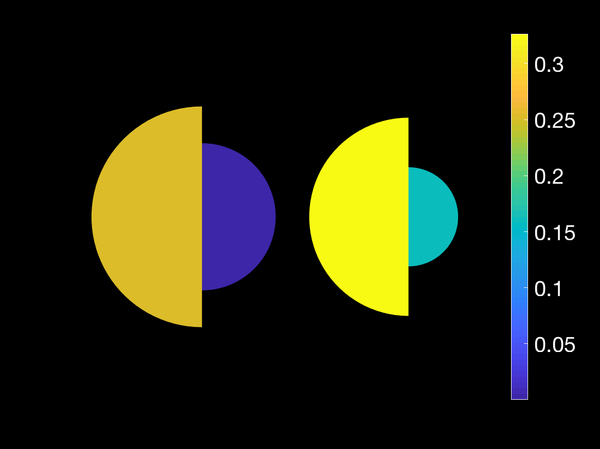
Figure 6: Two solutions with the Poisson’s ratio $\nu_{0}={1\over 6}$. The left solution is obtained for $\nu_{1}=0.4998$ while the left for $\nu_{1}=-1$. The colorcode represents the modulus of the displacement.

8 Conclusion

In this article, we have discussed the layer potentials and their corresponding integral operators on arbitrary bounded domains with Lipschitz boundary in the context of isotropic elasticity. We proved jump relations of layer potentials and the invertibility of the single layer boundary operator. In the particular case where the body is a unit ball, we present spectral properties of the boundary operators on the base of the vector spherical harmonics. We then derived a second-kind integral equation for isotropic elastic materials with spherical inclusions that was then discretized by employing the vector spherical harmonics as basis functions and exploiting the spectral properties to enhance efficiency of the discretization. In the last part, we effect some numerical tests to asses the properties of the method: the accuracy with respect to the degree of the vector spherical harmonics and the complexity of the computational cost with respect to the number of spherical inclusions. We also used the method to explore how the deformation of the elastic material is effected by the value of the Poisson’s ratio.

9 Aknowledgement

Benjamin Stamm acknowledges the funding from the German Academic Exchange Service (DAAD) from funds of the â Bundesministeriums für Bildung und Forschungâ (BMBF) for the project Aa-Par-T (Project-ID 57317909). Shuyang Xiang acknowledges the funding from the PICS-CNRS as well as the PHC PROCOPE 2017 (Project N37855ZK).

Appendix A: computation of the first few vector spherical harmonics

We first start considering the table of vector spherical harmonics up to the second order as listed below:

$$\ell=0: \qquad Y_{0,0}={1\over 2}\sqrt{1\over\pi},$$

$$\ell=1: \qquad Y_{1,-1}=\sqrt{3\over 4\pi}y, Y_{1,0} =\sqrt{3\over 4\pi}z, Y_{1,1} =\sqrt{3\over 4\pi}x,$$

$$\ell=2: \qquad Y_{2,-2}={1\over 2}\sqrt{15\over\pi}xy, Y_{2,-1} ={1\over 2}\sqrt{15\over\pi}yz, Y_{2,0} ={1\over 4}\sqrt{5\over\pi}(-x^{2}-y^{2}+2z^{2}),$$

$$\phantom{\qquad}Y_{2,1}={1\over 2}\sqrt{15\over\pi}xz, Y_{2,2} ={1\over 4}\sqrt{15\over\pi}(x^{2}-y^{2}).$$

This gives first the obvious result that

$$\ell=0:\qquad V_{0,0}=-{1\over 2}\sqrt{1\over\pi}(x,y,z)^{\top}\qquad\mbox{and}\qquad W_{00}=X_{00}=0.$$

Using the definition of the surface gradient (4.3), we obtain

$$\ell=1: \nabla_{\!\rm s}Y_{1,-1} =\sqrt{3\over 4\pi}\big{(}(0,1,0)-y(x,y,z)\big{)}^{\top},$$

$$\nabla_{\!\rm s}Y_{1,0} =\sqrt{3\over 4\pi}\big{(}(0,0,1)-z(x,y,z)\big{)}^{\top},$$

$$\nabla_{\!\rm s}Y_{1,1} =\sqrt{3\over 4\pi}\big{(}(1,0,0)-x(x,y,z)\big{)}^{\top},$$

$$\ell=2: \nabla_{\!\rm s}Y_{2,-2} ={1\over 2}\sqrt{15\over\pi}\big{(}(y,x,0)-2xy(x,y,z)\big{)}^{\top},$$

$$\nabla_{\!\rm s}Y_{2,-1} ={1\over 2}\sqrt{15\over\pi}\big{(}(0,z,y)-2yz(x,y,z)\big{)}^{\top},$$

$$\nabla_{\!\rm s}Y_{2,0} ={1\over 2}\sqrt{5\over\pi}\big{(}(-x,-y,2z)-(-x^{2}-y^{2}+2z^{2})(x,y,z)\big{)}^{\top},$$

$$\nabla_{\!\rm s}Y_{2,1} ={1\over 2}\sqrt{15\over\pi}\big{(}(z,0,x)-2xz(x,y,z)\big{)}^{\top},$$

$$\nabla_{\!\rm s}Y_{2,2} ={1\over 2}\sqrt{15\over\pi}\big{(}(x,-y,0)-(x^{2}-y^{2})(x,y,z)\big{)}^{\top}.$$

The spherical harmonics $V_{\ell m}$ up to order 2 are then given as follows

$$\ell=0: V_{0,0} =-{1\over 2}\sqrt{1\over\pi}(x,y,z)^{\top},$$

$$\ell=1: V_{1,-1} =\sqrt{3\over 4\pi}\big{(}(0,1,0)-2y(x,y,z)\big{)}^{\top},$$

$$V_{1,0} =\sqrt{3\over 4\pi}\big{(}(0,0,1)-2z(x,y,z)\big{)}^{\top},$$

$$V_{1,1} =\sqrt{3\over 4\pi}\big{(}(1,0,0)-2x(x,y,z)\big{)}^{\top},$$

$$\ell=2: V_{2,-2} ={1\over 2}\sqrt{15\over\pi}\big{(}(y,x,0)-5xy(x,y,z)\big{)}^{\top},$$

$$V_{2,-1} ={1\over 2}\sqrt{15\over\pi}\big{(}(0,z,y)-5yz(x,y,z)\big{)}^{\top},$$

$$V_{2,0} ={1\over 2}\sqrt{5\over\pi}\big{(}(-x,-y,2z)-{5\over 2}(-x^{2}-y^{2}+2z^{2})(x,y,z)\big{)}^{\top},~{}$$

$$V_{2,1} ={1\over 2}\sqrt{15\over\pi}\big{(}(z,0,x)-5xz(x,y,z)\big{)}^{\top},$$

$$V_{2,2} ={1\over 2}\sqrt{15\over\pi}\big{(}(x,-y,0)-{5\over 2}(x^{2}-y^{2})(x,y,z)\big{)}^{\top}.$$

The spherical harmonics $W_{\ell m}$ up to order 2 are given by

$$\ell=0: W_{0,0} =0,$$

$$\ell=1: W_{1,-1} =\sqrt{3\over 4\pi}(0,1,0)^{\top}, W_{1,0} =\sqrt{3\over 4\pi}(0,0,1)^{\top}, W_{1,1} =\sqrt{3\over 4\pi}(1,0,0)^{\top},$$

$$\ell=2: W_{2,-2} ={1\over 2}\sqrt{15\over\pi}(y,x,0)^{\top}, W_{2,-1} ={1\over 2}\sqrt{15\over\pi}(0,z,y)^{\top}, W_{2,0} ={1\over 2}\sqrt{5\over\pi}(-x,-y,2z)^{\top},$$

$$W_{2,1} ={1\over 2}\sqrt{15\over\pi}(z,0,x)^{\top}, W_{2,2} ={1\over 2}\sqrt{15\over\pi}(x,-y,0)^{\top}.$$

And finally, the spherical harmonics $X_{\ell m}$ up to order 2 are given by

$$\ell=0: X_{0,0} =0,$$

$$\ell=1: X_{1,-1} =\sqrt{3\over 4\pi}(-z,0,x)^{\top}, X_{1,0} =\sqrt{3\over 4\pi}(y,-x,0)^{\top},$$

$$X_{1,1} =\sqrt{3\over 4\pi}(0,z,-y)^{\top},$$

$$\ell=2: X_{2,-2} ={1\over 2}\sqrt{15\over\pi}(-xz,yz,x^{2}-y^{2})^{\top}, X_{2,-1} ={1\over 2}\sqrt{15\over\pi}(y^{2}-z^{2},-xy,xz)^{\top},$$

$$X_{2,0} ={1\over 2}\sqrt{5\over\pi}(3yz,-3xz,0)^{\top}, X_{2,1} ={1\over 2}\sqrt{15\over\pi}(xy,z^{2}-x^{2},-yz)^{\top},$$

$$X_{2,2} ={1\over 2}\sqrt{15\over\pi}(yz,xz,-2xy)^{\top}.$$

Appendix B: Entries of matrices $A_{\mathcal{D},\ell}^{in}$ and $A_{\mathcal{D},\ell}^{out}$

The coefficients in $A_{\mathcal{D},\ell}^{in}$ and $A_{\mathcal{D},\ell}^{out}$ are given as follows:

$$a^{in,\mathcal{D},\ell}_{11} =-{(\ell+2)\big{(}(3\ell+2)\mu+(\ell+1)\lambda\big{)}\big{(}(3\ell+1)\mu+\ell\lambda\big{)}\over(2\ell+3)(2\ell+1)^{2}\mu(2\mu+\lambda)},$$

$$a^{in,\mathcal{D},\ell}_{21,1} =-{(\ell+1)(\ell+2)\big{(}(3\ell+2)\mu+(\ell+1)\lambda\big{)}(\mu+\lambda)\over 2(2\ell+1)^{2}(2\mu+\lambda)},$$

$$a^{in,\mathcal{D},\ell}_{21,2} ={(\ell+1)(\ell+2)\big{(}(3\ell+2)\mu+(\ell+1)\lambda\big{)}(\mu+\lambda)\over 2(2\ell-1)(2\ell+1)\mu(2\mu+\lambda)},$$

$$a^{in,\mathcal{D},\ell}_{12} =-{\ell(\ell-1)(\mu+\lambda)\big{(}(3\ell+1)\mu+\ell\lambda\big{)}\over(2\ell+3)(2\ell+1)^{2}\mu(2\mu+\lambda)},$$

$$a^{in,\mathcal{D},\ell}_{22,1} =-{\ell(\ell-1)(\ell+1)(\mu+\lambda)^{2}\over 2(2\ell+1)^{2}\mu(2\mu+\lambda)},$$

$$a^{in,\mathcal{D},\ell}_{22,2} ={(\ell^{3}+24\ell^{2}-5\ell-8)\mu^{2}+2(\ell^{3}+6\ell^{2}-2\ell-2)\mu\lambda+(\ell^{3}-\ell)\lambda^{2}\over(2\ell-1)(2\ell+1)\mu(2\mu+\lambda)},$$

and

$$a^{out,\mathcal{D},l}_{11,1} ={(\ell+1)\big{(}(\ell^{2}+10\ell+4)\mu^{2}+(2\ell^{2}+8\ell+2)\mu\lambda+(\ell^{2}+\ell)\lambda\big{)}\over 2(2\ell+1)(2\ell+3)\mu(2\mu+\lambda)},$$

$$a^{out,\mathcal{D},\ell}_{11,2} =-{\ell(\ell+1)(\ell+2)(\mu+\lambda)^{2}\over 2(2\ell+1)^{2}\mu(2\mu+\lambda)},$$

$$a^{out,\mathcal{D},\ell}_{21} ={(\ell+1)(\ell+2)(\mu+\lambda)\big{(}(3\ell+2)\mu+(\ell+1)\lambda\big{)}\over(2\ell-1)(2\ell+1)^{2}\mu(2\mu+\lambda)},$$

$$a^{out,\mathcal{D},\ell}_{12,1} =-{\ell(\ell-1)(\mu+\lambda)\big{(}(3\ell+1)\mu+l\lambda\big{)}\over 2(2\ell+3)(2\ell+1)\mu(2\mu+\lambda^{2})},$$

$$a^{out,\mathcal{D},\ell}_{12,2} ={\ell(\ell-1)\big{(}(3\ell+1)\mu+\ell\lambda\big{)}(\mu+\lambda)\over 2(2\ell+1)(2\ell+3)\mu(2\mu+\lambda)},$$

$$a^{out,\mathcal{D},\ell}_{22} ={(\ell-1)\big{(}(3\ell+1)\mu+\ell\lambda\big{)}\big{(}(3\ell+2)\mu+(\ell+1)\lambda\big{)}\over(2\ell-1)(2\ell+1)^{2}\mu(2\mu+\lambda)}.$$

References

- [1] Bower. A. Lecture notes: EN224: Linear Elasticity. Division of Engineering, Brown University, 2005.
- [2] R.G. Barrera, G.A. Estévez, and J. Giraldo. Vector spherical harmonics and their application to magnetostatics. Eur. J. Phys., 6(287-294), 1985.
- [3] H. D. Bui. An integral eqautions method for solving the problem of a plane crack of arbitary shape. J. Mech. Phys. Solids, 25:29–39, 1997.
- [4] E. Cancès, V. Ehrlacher, F. Legoll, B. Stamm, and S. Xiang. An embedded corrector problem for homogenization. Part I: Theory. to appear in SIAM MMS, 2020.
- [5] Eric Cancès, Virginie Ehrlacher, Frédéric Legoll, Benjamin Stamm, and Shuyang Xiang. An embedded corrector problem for homogenization. Part II: Algorithms and discretization. Journal of Computational Physics, page 109254, 2020.
- [6] B. Carrascal, P. Estevez, Lee, and V. Lorenzo. Vector spherical harmonics and their application to classical electrodynamics. Eur. J. Phys., 12(184-191), 1991.
- [7] Haxton D.J. Lebedev discrete variable representation. Journal of Physics B: Atomic, Molec- ular and Optical Physics, (40):23, 2007.
- [8] Corona E. and Veerapaneni S. Boundary integral equation analysis for suspension of spheres in Stokes flow. Journal of Computational Physics, 362:327–345, 2018.
- [9] E.L.Hill. The theory of vector spherical harmonics. Am. J. Phys, 22(211- 214), 1954.
- [10] Weinberg. E. J. Monopole vector spherical harmonics. Phys. Rev. D, 49:1086–1092, 1994.
- [11] V.V. Jikov, S.M. Kozlov, and O.A. Oleinik. Homogenization of differential operators and integral functionals. Springer, Berlin, 1994.
- [12] Phani K. K. and Sanyal D. The relations between the shear modulus, the bulk modulus and Young’s modulus for porous isotropic ceramic material. Mater. Sci. Eng. A., 490(1):305–312, 2008.
- [13] V D Kupradze. Progress in solid mechanics / Dynamical problems in elasticity., volume 3. Amsterdam : North-Holland Publishing, 1963.
- [14] Eric B. Lindgren, Anthony J. Stace, Etienne Polack, Yvon Maday, Benjamin Stamm, and Elena Besley. An integral equation approach to calculate electrostatic interactions in many-body dielectric systems. Journal of Computational Physics, 371:712–731, 2018.
- [15] Leroy. Y. M. Introduction to the finite-element method for elastic and elasto-plastic solids. In Mechanics of Crustal Rocks, pages 157–239. Springer, Vienna, 2011.
- [16] T.M. MacRobert. Spherical harmonics: an elementary treatise on harmonic functions, with applications. Pergamon Press, 1967.
- [17] William McLean. Strongly elliptic systems and boundary integral equations. Cambridge university press, 2000.
- [18] Mott P.H. and Roland C.M. Limits to Poisson’s ratio in isotropic materials. Phys. Rev. B, 80(132104), 2009.
- [19] Falk. R. S. Lecture notes: Finite element method for linear elasticity. Department of Mathematics - Hill CenterRutgers, The State University of New Jersey, 2008.
- [20] Stefan A Sauter and Christoph Schwab. Boundary element methods. In Boundary Element Methods, pages 183–287. Springer, 2010.
- [21] Olaf Steinbach. Numerical approximation methods for elliptic boundary value problems: finite and boundary elements. Springer Science & Business Media, 2007.
- [22] Kushch V.I. Effective Properties of Heterogeneous Materials, chapter 2, pages 97–197. Springer, February 2013.
- [23] Hobson E. W. The theory of spherical and ellipsoidal harmonics. Chelsea Pub. Co., 1955.