GMRES with Singular Vector Approximations

Abstract

This paper has proposed the GMRES that augments Krylov subspaces with a set of approximate right singular vectors. The proposed method suppresses the error norms of a linear system of equations. Numerical experiments comparing the proposed method with the Standard GMRES and GMRES with eigenvectors methods[3] have been reported for benchmark matrices.

1 Introduction

The GMRES method is well-known for solving $Ax=b,$ a large sparse system of linear equations, especially, when an approximate solution is sufficient [5]. Nonetheless, the error norms of approximate solutions in GMRES need not be smaller; See [1, Example-1]. Prompted by this, Weiss proposed an algorithm that minimizes error norms, The Generalized Minimal Error method (GMERR)[7]. Ehrig and Deuflhard studied convergence properties of GMERR and developed an algorithm that has an implementation similar to GMRES [1].

Later, A stable variant of GMERR proposed using Householder transformations and has observed that the full version of GMERR may be effective in reducing the error, but its performance is not competitive to GMRES [4]. Although CGNR minimizes both error and residual norms, its convergence depends on the square of the condition number of $A$ [2].

This paper develops a tool that can combine to standard restarting GMRES, and reduce both error and residual norms. The tool augments the Krylov subspaces in restarting GMRES with a set of approximate right singular vectors.

The following is the outline of this paper: In Section-2, we present the GMRES method. Section-3 develops the said tool, and analyzes the convergence properties of the GMRES with approximate Singular vectors method. Section-4 gives implementation details of the algorithm proposed in section-3. Section-5 reports the results of numerical experiments on some benchmark matrices. Section-6 concludes the paper.

2 GMRES

Consider the following system of linear equations:

$$Ax=b,A\in\mathcal{C}^{~{}n\times n},b~{}\in~{}\mathcal{C}^{~{}n},x\in\mathcal{C}^{~{}n}.$$

Let $x0\in\mathcal{C}^{n}$ be an arbitrarily chosen initial approximation to the solution of the above problem. Without loss of generality, it is assumed throughout the paper that $x0=0$ so that $r_{0}=b.$ Then, at $i^{th}$ iteration of GMRES an approximate solution belongs to the Krylov subspace:

$$\mathcal{K}_{i}(A,b)~{}=~{}span\{b,Ab,\cdots,A^{i-1}b\},$$

and is of minimal residual norm:

$$\|r_{i}\|=\min_{x\in\mathcal{K}_{i}(A,b)}\|b-Ax\|.$$ (2.1)

The GMRES method solves this minimization problem by generating the matrix $V_{i}=\begin{bmatrix}v_{1}~{}v_{2}~{}\cdots~{}v_{i}\end{bmatrix}$ in successive iterations, using the following recurrence relation:

$$AV_{i}=V_{i}H_{i}+h_{i+1,i}v_{i+1}e_{i}^{\ast},~{}~{}\mbox{where}~{}~{}v_{1}=\frac{b}{\|b\|},$$ (2.2)

and $H_{i}$ is an unreduced upper Hessenberg matrix of order $i.$ Here, a vector $v_{i+1}\perp v_{j}$ for $j=1,2,\cdots i,$ and $\|v_{i+1}\|=1.$ Thus, vectors $v_{j}$ for $j=1,2,\cdots i$ form an orthonormal basis for the Krylov subspace $\mathcal{K}_{i}(A,b).$

Next, by using the equation (2.2), GMRES recasts the minimization problem in (2.1) into the following:

$$z_{i}=\arg\min_{x\in\mathcal{C}^{i}}\|b-AV_{i}x\|=\arg\min_{x\in\mathcal{C}^{i}}\|\beta V_{i+1}e_{1}-V_{i+1}\tilde{H_{i}}x\|,$$

where $\beta=\|b\|,$ and $\tilde{H_{i}}$ is an upper Hessenberg matrix obtained by appending the row $[0~{}0~{}\cdots~{}h_{i+1,i}]$ at the bottom of the matrix $H_{i}.$ As columns of the matrix $V_{i+1}$ are orthonormal, the above least squares problem is equivalent to the following problem:

$$z_{i}=\arg\min_{x\in\mathcal{C}^{i}}\|\beta e_{1}-\tilde{H_{i}}x\|.$$

GMRES solves this problem for the vector $z_{i}$ by using the $QR$ decomposition of the matrix $\tilde{H_{i}}.$ Note that a vector $V_{i}z_{i}$ minimizes the associated residual norm due to the equation (2.1). Thus, the sequence of residual norms $\{\|b-AV_{i}z_{i}\|_{2}\}$ in GMRES is monotonically decreasing. However, the corresponding sequence of error norms may not decrease monotonically. To tackle this, in the following sections, we augment the Krylov subspace in the GMRES method with a vector space containing approximate singular vectors.

3 Motivation:

In this section, we are addressing the augmentation of a Krylov subspace in GMRES with the singular vectors. The following lemma explains the motivation behind this.

Lemma 1.

Let $z$ be a right singular vector of a matrix $A$ corresponding to the singular value $\sigma,$ and $x0$ be an approximate solution of a linear system of equations $Ax=b.$ Then, a solution of the following minimization problem

$$\alpha=\arg\min_{k\in\cal{C}}\|b-Ax0-kAz\|,$$ (3.1)

is the solution of the minimization problem

$$\alpha=\arg\min_{k\in\cal{C}}\|x-x0-kz\|.$$ (3.2)

Proof.

Let $\alpha$ be a solution of the minimization problem (3.1). By using $Ax=b,$ this implies $\alpha=\frac{\langle Ax-Ax0,Az\rangle}{\|Az\|^{2}}.$ Further, by using $\|z\|_{2}=1$ and $A^{\ast}Az=\sigma^{2}z$ from the hypothesis, we have $\alpha=\frac{\langle x-x0,z\rangle}{\|z\|^{2}}.$ Equivalently, this gives

$$\langle x-x0-\alpha z,z\rangle=\langle x-x0,z\rangle-\alpha\|z\|^{2}=0.$$

Thus, a vector $x-x0-\alpha z$ is orthogonal to the vector space spanned by the vector $z.$ Therefore, $\alpha$ is a solution of the minimization problem (3.2). ∎

The above lemma has shown an advantage of the singular vectors that they reduce both residual and error norms. Now the following two questions arise when augmenting the Krylov subspace in GMRES with a vector space spanned by singular vectors. The first question is computing a singular vector of a sparse matrix requires more computation than finding the solution of a sparse linear system of equations, in general. The second question to address is singular vectors corresponding to what singular values are better to augment Krylov subspaces in GMRES.

Usage of an approximate singular vector in the augmentation process instead of an exact singular vector resolves the first problem. The following theorem discusses the effect of this usage.

Theorem 1.

Let a matrix $V_{m}$ have orthonormal columns and $x0$ be an approximate solution of a linear system of equations $Ax=b.$ Assume that $x-x0$ is in the range space of $V_{m}$ and $z$ is a right singular vector of the matrix $AV_{m}$ corresponding to its singular value $\sigma.$ Then a solution of the following minimization problem

$$\alpha=\arg\min_{k\in\cal{C}}\|b-Ax0-kAV_{m}z\|$$ (3.3)

is the solution of the minimization problem:

$$\alpha=\arg\min_{k\in\cal{C}}\|x-x0-kV_{m}z\|.$$ (3.4)

Proof.

Let $x-x0=V_{m}y.$ Note that if $y$ is a zero vector then $x0$ is an exact solution of the linear system $Ax=b.$ Assume that $y$ is a non-zero vector. Now, $\alpha,$ a solution of the minimization problem (3.3) is

$$\alpha=\frac{\langle Ax-Ax0,AV_{m}z\rangle}{\|AV_{m}z\|^{2}}=\langle y,z\rangle=\langle x-x0,V_{m}z\rangle.$$ (3.5)

The above equation has used the facts that $V_{m}^{\ast}A^{\ast}AV_{m}z=\sigma^{2}z,$ and $V_{m}^{\ast}V_{m}$ is an Identity matrix. Therefore, by using the same lines of proof as in the previous lemma, $\alpha$ is a solution of the error minimization problem (3.4). ∎

The Theorem-1 says that if $x-x0$ is in the Krylov subspace spanned by the columns of $V_{m}$ a singular vector of $AV_{m}$ will serve the purpose of a singular vector of $A$ in the augmentation process. However, the error vector $x-x0$ may not lie entirely in the said subspace, in general. In this case, the following theorem establishes a relationship between the solutions of minimization problems (3.3) and (3.4).

Theorem 2.

Let $x0$ be an approximate solution of the linear system of equations $Ax=b$ and $\sigma,z$ are same as in the previous theorem. Assume that $\alpha_{1},$ $\alpha_{2}$ are solutions of the minimization problems (3.3) and (3.4) respectively. Then,

$$\|x-x0-\alpha_{1}V_{m}z\|^{2}-\|x-x0-\alpha_{2}V_{m}z\|^{2}=\frac{|\langle x-x0,(A^{\ast}A-\sigma^{2}I)V_{m}z\rangle|^{2}}{\sigma^{4}}.$$ (3.6)

Proof.

Note that $x-x0=V_{m}V_{m}^{\ast}(x-x0)+(I-V_{m}V_{m}^{\ast})(x-x0).$ By using $Ax=b$ and this, the solution $\alpha_{1}$ of the minimization problem (3.3) can be written as

$$\alpha_{1}=\frac{\langle AV_{m}V_{m}^{\ast}(x-x0)+A(I-V_{m}V_{m}^{\ast})(x-x0),AV_{m}z\rangle}{\|AV_{m}z\|^{2}}.$$

On substituting the equation (3.5) this yields

$$\alpha_{1}=\langle x-x0,V_{m}z\rangle+\frac{\langle x-x0,(I-V_{m}V_{m}^{\ast})A^{\ast}AV_{m}z\rangle}{\|AV_{m}z\|^{2}}.$$

Further, by using $V_{m}^{\ast}A^{\ast}AV_{m}z=\sigma^{2}z,$ this gives

$$\alpha_{1}=\langle x-x0,V_{m}z\rangle+\frac{\langle x-x0,(A^{\ast}A-\sigma^{2}I)V_{m}z\rangle}{\|AV_{m}z\|^{2}}=\big{\langle}x-x0,\frac{A^{\ast}AV_{m}z}{\sigma^{2}}\big{\rangle}.$$ (3.7)

The above equation used the fact that $\|AV_{m}z\|^{2}=\sigma^{2}.$ As $\|V_{m}z\|_{2}=1$ and $\alpha_{2}$ is the solution of an error minimization problem (3.4), we have $\alpha_{2}=\langle x-x0,V_{m}z\rangle,$ and

$$\|x-x0-\alpha_{1}V_{m}z\|^{2}-\|x-x0-\alpha_{2}V_{m}z\|^{2}=|\alpha_{1}-\alpha_{2}|^{2}\|V_{m}z\|^{2}=|\alpha_{1}-\alpha_{2}|^{2}.$$

Now, observe from the equation (3.7) that

$$\alpha_{1}-\alpha_{2}=\big{\langle}x-x0,\frac{(A^{\ast}A-\sigma^{2}I)V_{m}z}{\sigma^{2}}\big{\rangle},$$ (3.8)

and substitute it in the previous equation. It gives the equation (3.6). Hence, we proved the theorem. ∎

From $V_{m}^{\ast}A^{\ast}AV_{m}z=\sigma^{2}z$ note that $(A^{\ast}A-\sigma^{2}I)V_{m}z=(I-V_{m}V_{m}^{\ast})(A^{\ast}A-\sigma^{2}I)V_{m}z.$ On substituting this in the right-hand side of the equation (3.6), it is easy to see that the difference between $\|x-x0-\alpha_{1}V_{m}z\|^{2}$ and $\|x-x0-\alpha_{2}V_{m}z\|^{2}$ was only due to components orthogonal to $V_{m}$ in $x-x0,$ that means, ”The components from the column space of $V_{m}$ are optimally balanced in the error vector $x-x0-\alpha_{1}V_{m}z."$ Thus, augmenting a search subspace in GMRES with a singular vector approximation will accelerate the convergence of approximate solutions. This fact motivates us to augment the Krylov subspace at each run in the restarting GMRES with the singular vector approximations as explained in the following paragraph.

Let $e_{m}^{(i)}$ denotes an error vector, and the columns of $V_{m}^{(i)}$ span the search subspace at the $i^{th}$ run of restarting GMRES. Suppose $z$ is a right singular vector of $AV_{m}^{(i)}$ and it augments the column space of $V_{m}^{(i+1)}$ at the $(i+1)^{th}$ run. Then, the Theorem-2 and the previous paragraph says that the components of the column space of $V_{m}^{(i)}$ are optimally balanced in the error vector that corresponds to the vector minimizing a residual norm over Range$(V_{m}^{(i+1)},V_{m}^{(i)}z).$

Next, the following theorem is required to answer the second question that we arose before, approximate singular vectors corresponding to what singular values are better to augment the Krylov subspace in GMRES. The proof will follow the lines of Sections 3 and 4 in [8].

Theorem 3.

Let a subspace range of $Y_{k}$ be augmenting the Krylov subspace $\mathcal{K}_{m}(A,r_{0}),$ where $Y_{k}\in C^{n\times k}$ and $m+k<n.$ Assume that $z\in Y_{k},$ and $q(A)$ is a polynomial in $A$ of degree $m$ such that $q(0)=0.$ Let $r_{s}:=r_{0}-y$ be an optimal residual over the space Range$(AV_{m},AY_{k}),$ where $y:=\|r_{0}\|q(A)v+Az.$ Then

$$\frac{\|r_{s}\|^{2}}{\|r_{0}\|^{2}}\leq 1-\min_{w\in S_{n}}\frac{|w^{\ast}q(A)w|^{2}+\|w^{\ast}AY_{k}\|^{2}}{\|q(A)\|^{2}+\|AY_{k}\|_{F}^{2}},$$ (3.9)

where $S_{n}$ denotes the unit sphere in $C^{n},$ and $\|~{}.~{}\|_{F}$ is the Frobenius norm.

Proof.

Let $U:=(q(A)v,AY_{k})$ is a matrix of full rank. Then, $P=U(UU^{\ast})^{-1}U^{\ast}$ defines an orthogonal projection onto the space $\textbf{Range}(q(A)v,AY_{k}).$ Thus,

$$Pr_{0}\in\textbf{Range}(q(A)v,AY_{k}).$$

Since $q(A)v\in AV_{m},$ and $r_{s}:=r_{0}-y$ is an optimal residual over $\textbf{Range}(AV_{m},AY_{k}),$ this implies

$$\|r_{s}\|^{2}\leq\|r_{0}-Pr_{0}\|^{2}=\|(I-P)r_{0}\|^{2}.$$

This gives

$$\frac{\|r_{s}\|^{2}}{\|r_{0}\|^{2}}\leq\|(I-P)\frac{r_{0}}{\|r_{0}\|}\|^{2}=\|(I-P)v\|^{2}=1-v^{\ast}Pv.$$

By using $P=U(UU^{\ast})^{-1}U^{\ast}$ the above equation gives the following:

$$\frac{\|r_{s}\|^{2}}{\|r_{0}\|^{2}}\leq 1-\|U^{\ast}v\|^{2}\lambda_{min}(U^{\ast}U)^{-1}\leq 1-\frac{\|U^{\ast}v\|^{2}}{\lambda_{max}(U^{\ast}U)}\leq 1-\frac{\|U^{\ast}v\|^{2}}{Trace(U^{\ast}U)}.$$

Since $U=(q(A)v,AY_{k}),$ we have $\|U^{\ast}v\|^{2}=|v^{\ast}q(A)v|^{2}+\|v^{\ast}AY_{k}\|^{2}$ and $Trace(U^{\ast}U)=\|q(A)v\|^{2}+\|AY_{k}\|_{F}^{2}.$ Substituting these inequalities in the above equation gives the following:

$$\frac{\|r_{s}\|^{2}}{\|r_{0}\|^{2}}\leq 1-\frac{|v^{\ast}q(A)v|^{2}+\|v^{\ast}AY_{k}\|^{2}}{\|q(A)v\|^{2}+\|AY_{k}\|_{F}^{2}}\leq 1-\frac{|v^{\ast}q(A)v|^{2}+\|v^{\ast}AY_{k}\|^{2}}{\|q(A)\|^{2}+\|AY_{k}\|_{F}^{2}}.$$

Here, the second inequality used the facts that $\|v\|_{2}=1$ and $\|q(A)v\|_{2}\leq\|q(A)\|_{2}.$ Now minimizing the numerator of the second term over $S_{n},$ the unit sphere in $C^{n},$ gives the equation (3.9). Hence, the theorem proved. ∎

From the Theorem-3 note that the norm of an updated residual $\|r_{s}\|$ deviates more from $\|r_{0}\|$ when $\|AY_{k}\|_{F}$ is smaller. It is well known that $\|AY_{k}\|_{F}$ is small when columns of $Y_{k}$ are right singular vectors corresponding to smaller singular values of $A.$ This answers the second question that we arose before. The next section devises the GMRES with approximate singular vectors method. The new algorithm augments a Krylov subspace at each run with an approximate right singular vector from the previous run.

4 Implementation

Let $x0$ be an initial approximate solution of a linear system of equations $Ax=b,$ and $r_{0}=b-Ax0.$ Let $m$ be the dimension of a search subspace consists of $m-k$ dimensional Krylov subspace ${\cal K}_{m-k}(A,r_{0})$ and $k<m$ approximate singular vectors. Let $W$ be a matrix of order $n\times m.$ Assume that the first $(m-k)$ columns of $W$ form an orthonormal basis for the Krylov subspace ${\cal K}_{m-k}(A,r_{0})$ and its last $k$ columns are approximate singular vectors $y_{i},$ for $i=1,2,\cdots k.$

The new algorithm recursively constructs first $m-k$ columns of $W$ and an orthonormal basis matrix $Q$ of an $m$ dimensional search subspace. The matrices $W$ and $Q$ satisfy the following relation:

$$AW=Q\tilde{H},$$

where $\tilde{H}$ is an upper Hessenberg matrix of order $(m+1)\times m.$ Note that $Q$ is a matrix of order $n\times(m+1)$ and its first $m-k+1$ columns are formed using the Arnoldi recurrence relation. The last $k$ columns of it are formed by successively orthogonalizing the vectors $Ay_{i}$ for $i=1,2,.....,k$ against its previous columns. Further, notice that $Q^{\ast}r_{0}$ is a multiple of a first coordinate vector.

Similar to the GMRES algorithm, the new algorithm computes an orthogonal matrix $P$ of order $(m+1)$ and an upper triangular matrix $R$ of order $(m+1)\times m$ such that

$$P\tilde{H}=R.$$

Then, it finds a vector $d$ such that $\|r\|=\|b-A(x0+Wd)\|$ is minimum, and updates an approximate solution to x̂$:=x0+Wd.$ Note that

$$\|r\|=\|b-A(x0+Wd)\|=\|r_{0}-AWd\|=\|r_{0}-Q\tilde{H}d\|$$

$$=\|Q^{\ast}r_{0}-\tilde{H}d\|=\|PQ^{\ast}r_{0}-Rd\|.~{}~{}~{}~{}~{}~{}~{}~{}~{}~{}~{}~{}~{}~{}~{}~{}~{}~{}~{}$$

As $R$ is an upper triangular matrix of order $(m+1)\times m$ and $\|PQ^{\ast}r_{0}-Rd\|$ is minimum, the new method gives the minimal solution by solving for $d$ that makes the first $m$ entries of $PQ^{\ast}r_{0}-Rd$ zero. Hence, $\|r\|$ is equal to the magnitude of the last entry of $PQ^{\ast}r_{0}.$ Therefore, in the new method, $\|r\|$ is a byproduct and does not require any extra computation.

Next, We wish to find approximate right singular vectors of $A$ from the subspace spanned by $W$ to augment the search subspace in the next run. For this, we find eigenvectors corresponding to the $k$ smaller eigenvalues of the matrix $W^{\ast}A^{\ast}AW.$ A little calculation is required to compute this matrix, because of

$$G:=W^{\ast}A^{\ast}AW=\tilde{H}^{\ast}Q^{\ast}Q\tilde{H}=\tilde{H}^{\ast}\tilde{H}=R^{\ast}R.$$

We used the Matlab command ”eigs” to solve the eigenvalue problem for $G.$

The implementation of our new method is as follows. For simplicity, a listing of the algorithm has done for the second and subsequent runs.

One restarted run of GMRES with singular vectors

1. Initial definitions and calculations: The Krylov subspace has dimension m-k, k is the number of approximate eigenvectors. Let $q_{l}=\frac{r_{0}}{\|r_{0}\|}$ and $w_{l}=q_{l}.$ Let $y_{1},y_{2},...,y_{k}$ be the approximate singular vectors. Let $W_{m+i}=y_{i},$ for $i=1,2,...,k.$
2. Generation of Arnoldi vectors: For $j=1,2,...,m$ do:

$h_{i,j}=\langle Aq_{j},q_{i}\rangle,~{}i=1,2,...,j$,

$\hat{q}_{j+1}=Aq_{j}-\displaystyle\sum\limits_{i=1}^{j}h_{i,j}q_{i},$

$h_{j+1,j}=\|\hat{q}_{j+1}\|,$ and

$q_{j+1}=\hat{q}_{j+1}/h_{j+1,j}.$

If $j<m-k,$ let $w_{j+1}=q_{j+1}.$

3.Addition of approximate singular vectors: For $j=m-k+1,m-k+2,...m$,do:

$h_{i,j}=\langle Aw_{j},q_{i}\rangle,$  $i=1,2,...,j$,

$\hat{q}_{j+1}=Aw_{j}-\displaystyle\sum\limits_{i=1}^{j}h_{i,j}q_{i},$

$h_{j+1,j}=\|{\hat{q}_{j+1}}\|,$ and

$q_{j+1}=\frac{\hat{q}_{j+1}}{h_{j+1,j}}.$

4. Form the approximate solution: Let $\beta=\|r_{0}\|.$ Find $d$ that minimizes $\|\beta e_{1}-\tilde{H}d\|$ for all $d\in{\cal R}^{m}$. The orthogonal factorization $P\tilde{H}=R$, for R upper triangular, is used. Then $\hat{x}=xo+Wd.$
5. Form the new approximate singular vectors: Calculate $G=R^{\ast}R.$ Solve $Gg_{i}=\sigma^{2}g_{i}$, for the appropriate $g_{i}.$ Form $y_{i}=Wg_{i}$ and $Ay_{i}=Q\tilde{H}g_{i}$.
6. Restart: Compute $r=b-A\hat{x}$; if satisfied with the residual norm then stop, else let $x0=\hat{x}$ and go to 2.

Only the Step-5 in the above algorithm is different from the GMRES with eigenvectors method. The GMRES with eigenvectors method requires the computation of both $F=W^{\ast}A^{\ast}W$ and $G$ [3], whereas the Step-5 in the above algorithm computes the only $G=W^{\ast}A^{\ast}AW.$ Hence, the above algorithm requires less computation and storage compared to the GMRES with eigenvectors method.

Next, we compare the GMRES with singular vectors and standard GMRES methods. For this, we follow the procedure that used in [3] to compare the standard GMRES and GMRES with eigenvectors methods. It compares only significant expenses.

Suppose the search subspace currently at hand is a Krylov subspace of dimension $j.$ If the search subspace expands with one more Arnoldi vector, then it requires one matrix-vector product. The orthogonalization requires about $2jn$ multiplications. Instead, if search subspace expanded with a singular vector approximation, no matrix-vector product is required. The other costs are approximately $4jn$ multiplications. It includes $2jn$ multiplications for orthogonalization and $2jn$ for computing $y_{i}$ and $Ay_{i}.$ Hence, GMRES with singular vectors requires $2jn$ extra multiplications compared to the standard GMRES, but at the cost of a matrix-vector product in GMRES that requires $n^{2}$ multiplications. In general, $2j<<n.$ Therefore, the GMRES with singular vectors method requires overall less computation than standard GMRES.

The GMRES with $k$ singular vector approximations method requires the storage of $m+2k+2$ vectors. This includes the storage of $2k$ vectors, $y_{i}$ and $Ay_{i}$ for $i=1,2,\cdots,k.$ However, the storage requirement for standard GMRES with $m+k$ dimensional Krylov subspace is $m+k+2$ vectors. Thus, the GMRES with singular vectors method requires extra storage compared to standard GMRES. Since $k<<m$ this extra storage is often not a problem.

5 Examples

In the following, GMRES-SV(m,k) indicates that at each run $k$ approximate singular vectors from the previous run augment Krylov subspace of dimension $m-k.$ Similarly, GMRES-HR(m,k) indicates the augmentation of approximate eigenvectors those obtained using the Harmonic Rayleigh-Ritz process to a Krylov subspace. Moreover, in the first run of both the methods search subspace is a Krylov subspace of dimension $m$ .

In each of the example, we compare GMRES-SV(m,k) with GMRES-HR(m,k), GMRES(m), and GMRES(m+k). Here for GMRES, the number in the parenthesis represents the dimension of a Krylov subspace at each run. Note that the dimension of search subspaces in GMRES(m), GMRES-SV(m,k) and GMRES-HR(m,k) are same, and in GMRES(m+k) the search subspace at each run requires nearly the same storage as that of GMRES-SV(m,k) and GMRES-HR(m,k).

In all numerical examples, the right-hand sides have all entries $1.0,$ unless mentioned otherwise. The initial guesses $x0$ are zero vectors. Further, we stopped each algorithm when $\|r\|/\|b\|$ reduced below the fixed tolerance $10^{-8}.$ All experiments have been carried out using MATLAB R2016b on intel core i7 system with $3.40GHZ$ speed.

Example 1.

This example is same as the example-1 in [7]. The linear system results from the discretization of one dimensional Laplace equation. The coefficient matrix $A$ is a symmetric tridiagonal matrix of dimension $1000,$ and the right-hand side vector is $(1~{}0~{}0~{}\cdots~{}0~{}1)^{\prime}$. The entry on the main diagonal of $A$ is $2$, whereas $−1$ is on the sub-diagonals of $A$. The matrix has eigenvalues $\lambda_{k}=2.(1-\cos\frac{k\pi}{1001})$ for $1\leq k\leq 1000$ and its condition number is $(1+\cos\frac{\pi}{1001})/(1-\cos\frac{\pi}{1001}).$

The Figure-1 depicts the convergence of residual norms and corresponding error norms in the GMRES-SV(20,4), GMRES-HR(20,4), GMRES(20), and standard GMRES(24) methods.

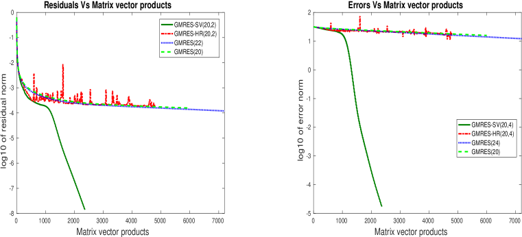
Figure 1: Magnitudes of $\frac{\|r\|}{\|b\|}$ with GMRES(20,4) singular vectors/eigenvectors, GMRES(24), and GMRES(20) (left). Absolute errors with GMRES(20,4) singular vectors/eigenvectors, GMRES(24), and GMRES(20) (right).

In GMRES-SV(20,4), $\|r\|/\|b\|$ drops to below the tolerance $10^{-8}$ in the $148^{th}$ run. It required $2365$ number of matrix-vector products. In the remaining three methods $\|r\|/\|b\|$ did not reached at least $10^{-4}$ even after $5000$ matrix-vector products. Here, the total number of matrix-vector products in all methods counted in a similar way as in [3].

Observe from the right part of Figure-1 that GMRES-SV(20,4) reduces error norms also to a far better extent than the remaining three methods. Here, error norm is the norm of an error vector, a difference between a solution obtained using ”backslash” command in Matlab and an approximate solution in an iterative method.

From the Figure-1, we observed that when residual norm drops below the tolerance $10^{-8},$ the $\log 10$ of an error norm in the GMRES-SV(20,4) is $-4.763.$ In the other three methods, at $5000^{th}$ matrix-vector product it is just near $1.244$. Therefore, this example illustrates the fact that the augmentation of a Krylov subspace with singular vectors reduces error norms and also the residual norms.

Example 2.

Consider the matrix $SHERMAN4$ that comes from Oil reservoir modeling. It is a real un-symmetric matrix of order $1104.$ The Matrix market provided the right-hand side vector. We compare GMRES-SV(20,4) (16 Krylov vectors and 4 approximate right singular vectors) with GMRES-HR(20,4), GMRES(20), and GMRES(24).

See left part of Figure 2 for the convergence of $log10$ of residual norms in all the methods.

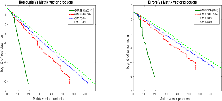
Figure 2: Magnitudes of $\frac{\|r\|}{\|b\|}$ with GMRES(20,4) singular vectors/eigenvectors, GMRES(24), and GMRES(20) (left). Absolute errors with GMRES(20,4) singular vectors/eigenvectors, GMRES(24), and GMRES(20) (right).

In GMRES-SV(20,4) the quantity $\|r\|/\|b\|$ reduced to below $10^{-8}$ at the $12^{th}$ run. The total number of matrix-vector products it required is $190.$ GMRES-HR(20,4) required $562$ matrix vector products to drop $\|r\|/\|b\|$ below the tolerance $10^{-8}.$ Thus, GMRES-HR had required nearly thrice the computation than the GMRES-SV method. Further, observe from the Figure-2 that GMRES-SV(20,4) is far better than GMRES(24) even though it used smaller search subspaces.

The right part of the Figure-2 compares error norms. When the residual norm reached the tolerance, the $\log 10$ of an error norm in GMRES-SV(20,4)is $-6.063,$ whereas it is $-5.063$ in GMRES-HR(20,4), and is equal to $-4.813,$ $-4.802$ in the GMRES(24) and GMRES(20) methods respectively. Therefore, for this example, the GMRES-SV method significantly reduced the error norm compared to the remaining three methods.

Example 3.

Consider the matrix $WATT1$ that came from petroleum engineering. It is a real un-symmetric matrix of order $1856$ with $11360$ non-zero entries. The right-hand side is the one provided by the Matrix Market. To see the performance of GMRES-SV with fewer approximate singular vectors, we have chosen $m=20$ and $k=2.$ Thus, we have used only two approximate singular vectors, which are less in number compared to the previous examples.

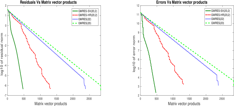
Figure 3: Magnitudes of $\frac{\|r\|}{\|b\|}$ with GMRES(20,2) singular vectors/eigenvectors, GMRES(22), and GMRES(20) (left). Absolute errors with GMRES(20,2) singular vectors/eigenvectors, GMRES(22), and GMRES(20) (right).

Using GMRES-SV(20,2), the ratio $\|r\|/\|b\|$ reached the required tolerance in the $30^{th}$ run, whereas in GMRES-HR(20,2), GMRES(22), and GMRES(20) it happened in $82^{nd},109^{th},$ and $143^{rd}$ run respectively. See Figure-3(left) for the comparison of $\log 10$ of residual norms in all the four methods.

Figure-3(right), compares the convergence of error norms in four methods. Observe from it that GMRES-SV(20,2) reduced the error norm to a better extent compared to the other three methods, even though it took fewer iterations for the convergence of $\|r\|/\|b\|.$ Also, it reduced residual norms as well.

Example 4.

This example has taken from [3]. It is a bidiagonal matrix of order $1000.$ The diagonal elements are $1,2,\cdots,1000$ in order. The super diagonal elements are $0.1s.$ We have chosen $m=20$ and $k=2$ for GMRES method with singular vectors. We used only two eigenvector approximations in GMRES-HR. We compare these two methods with GMRES(20) and GMRES(22).

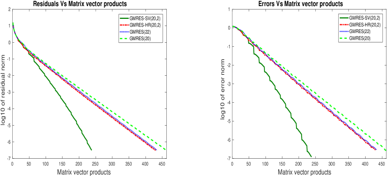
Figure 4: Magnitudes of $\frac{\|r\|}{\|b\|}$ with GMRES(20,2) singular vectors/eigenvectors, GMRES(22), and GMRES(20)(left). Absolute errors with GMRES(20,2) singular vectors/eigenvectors, GMRES(22), and GMRES(20) (right).

Figure-4(left), compares a ratio $\|r\|/\|b\|$ in these four different methods. Using GMRES-SV(20,2) $\|r\|/\|b\|$ had reached the desired tolerance in a $15^{th}$ run, whereas in GMRES-HR(20,2), GMRES(22), and GMRES(20), this ratio reduced below the tolerance in $27^{th},20^{th},$ and $24^{th}$ run, respectively. In the Figure-4(right), we compared the error norms in the four methods. Though the error is reduced up to the same order in all methods, the GMRES-SV(20,2) has taken less number of matrix-vector products. Further, observe that in GMRES-SV smaller error norm at each iteration accelerates the convergence of residual norms .

Above examples have shown that our new method is effective in accelerating the convergence of GMRES. It also shows that we can use singular vector approximations instead of eigenvector approximations to augment the search subspace. Further, example-1 has shown the superiority of the GMRES-SV method even in the case of near stagnation of error norms in standard GMRES.

We reported four typical examples in detail though computation carried out on several matrices available in the Matrix Market. The Table-1 reports a summary of results on eight other matrices with various base sizes. It is apparent from the table that the GMRES with singular vectors method performs better in reducing the error norms compared to standard GMRES and GMRES-HR.

Table 1: Summary results on other matrices

Matrix	Method	rhs	Initial vector	MVP	$\|r\|/\|b\|$	error
Add20	GMRES-SV(30,4)	NIST	Zeros(2395,1)	17*26	8.903030927585648e-09	6.249677395458858e-15
	GMRES(30)			27*30+23	9.951915432072370e-09	1.269588940989828e-14
	GMRES-HR(30,4)			24*26+9	9.859393321942817e-09	1.326769652866634e-14
Bcsstm12	GMRES-SV(30,4)	Ones(1473,1)	Zeros(1473,1)	7*26+21	9.735591826540923e-09	4.010655907680425e-05
	GMRES(30)			7*30+18	8.504590396065243e-09	3.371368967798073e-05
	GMRES-HR(30,4)			9*26+4	9.359680271393492e-09	3.454242536809857e-05
Cavity05	GMRES-SV(30,4)	NIST	Zeros(1182,1)	58*26+3	9.979063739097918e-09	8.864891034548036e-17
	GMRES(30)*			300*30	9.083509763407927e-06	4.366773990806636e-12
	GMRES-HR(30,4)*			300*30	4.188013345206927e-04	2.098667819011905e-10
Cavity10	GMRES-SV(30,4)	NIST	Zeros(2597,1)	107*26+2	9.748878041774344e-09	1.082459456375754e-14
	GMRES(30)*			300*30	1.480273732125253e-05	1.745590861026809e-09
	GMRES-HR(30,4)*			300*30	4.412649085564300e-05	5.202816341776465e-09
Cdde1	GMRES-SV(30,4)	Ones(961,1)	Zeros(961,1)	7*26+4	9.375985059553094e-09	9.904876436183557e-06
	GMRES(30)			28*30+24	9.903484254958585e-09	8.057216911709931e-05
	GMRES-HR(30,4)			42*26	9.784366641015672e-09	5.754305524376241e-05
$Orsreg_{1}$	GMRES-SV(30,4)	Ones(2205,1)	Zeros(2205,1)	9*26+18	9.636073229113061e-09	3.069738625094621e-08
	GMRES(30)			13*30+18	9.671973942415371e-09	8.655424850905282e-08
	GMRES-HR(30,4)			15*26+24	9.858474091767057e-09	7.314829956508281e-08
Sherman1	GMRES-SV(30,4)	NIST	Zeros(1000,1)	34*26+16	9.988703017482971e-09	3.073177766807258e-05
	GMRES(30)			103*30+21	9.987479947720702e-09	1.160914298556447e-04
	GMRES-HR(30,4)			35*26+1	8.658352412777792e-09	5.119874131512304e-05
$Watt_{2}$	GMRES-SV(30,4)	Ones(1856,1)	Zeros(1856,1)	40*26	9.956725136180967e-09	1.955980343013359e+03
	GMRES(30)			168*30+6	9.897399520154960e-09	6.004185029785801e+03
	GMRES-HR(30,2)			254*26	9.996375252736734e-09	7.072952057904888e+03

In Table-1, NIST refers to the right-hand side vector provided by Matrix Market website and GMRES* represents the non-convergence of the GMRES method even after 300 iterations. Moreover, for counting the number of matrix-vector products(MVP) we followed the same procedure as in [3]. In the above table $x*y+z$ means in each of the $x$ iterations, the specific method used $y$ MVPs and in the $(x+1)^{th}$ iteration, it used $z$ Matrix-Vector Products.

6 Conclusions

In this paper, a new augmentation procedure in GMRES has been proposed using approximate right singular vectors of a coefficient matrix. The proposed method has an advantage that it requires less computation compared to the GMRES with Harmonic Ritz vectors method. Unlike the augmentation method in [3], the proposed method reduces the error norms also to a better extent. Further, the proposed method involves the computation in real arithmetic for the matrices and right-hand side vectors in the real number system. Numerical experiments have been carried out on benchmark matrices. Results have shown the superiority of the proposed method over the standard GMRES and GMRES with Harmonic Ritz vectors methods.

References

References

- [1] R. Ehrig and Peter D.Euflhard, GMERR as an Error Minimizing Variant of GMRES, Preprint SC 97-63, Konrad-Zuse-Zentrum f̋ur Informationstechnik Berlin, 1997.
- [2] Chunguang Li, CGNR Is an Error Reducing Algorithm, SIAM Journal on Scientific Computing, 22:6 (2001), 2109-2112.
- [3] R.B. Morgan, A restarted GMRES method augmented with eigenvectors, SIAM J. Matrix Anal. Appl., 16:4 (1995), pp. 1154 - 1171.
- [4] M. Rozložník, R. Weiss, On the stable implementation of the generamized minimal error method, Journal of Computational and Applied Mathematics, 98 (1998), pp. 49 - 62.
- [5] Y. Saad, M.H. Schultz, GMRES: a generalized minimal residual algorithm for solving nonsymmetric linear systems, SIAM J. Sci. Stat. Comput., 7 (1986), pp. 856 - 869.
- [6] Y. Saad, Analysis of augmented Krylov subspace methods, SIAM J. Matrix. Anal. Appl., 18:2 (1997), pp. 435 -449.
- [7] R. Weiss, Error minimizing Krylov subspace methods, SIAM J.Sci.Comp., 15 (1994), pp.511-527.
- [8] J. Źitko, Some remarks on the restarted and augmented GMRES method, Electron. Trans. Numer. Anal., 31 (2008), pp. 221 - 227.