Noise in Boson Sampling and the threshold of efficient classical simulatability

Abstract

We study the quantum to classical transition in Boson Sampling by analysing how $N$-boson interference is affected by inevitable noise in an experimental setup. We adopt the Gaussian noise model of Kalai and Kindler for Boson Sampling and show that it appears from some realistic experimental imperfections. We reveal a connection between noise in Boson Sampling and partial distinguishability of bosons, which allows us to prove efficient classical simulatability of noisy no-collision Boson Sampling with finite noise amplitude $\epsilon$, i.e., $\epsilon=\Omega(1)$ as $N\to\infty$. On the other hand, using an equivalent representation of network noise as losses of bosons compensated by random (dark) counts of detectors, it is proven that for noise amplitude inversely proportional to total number of bosons, i.e., $\epsilon=O(1/N)$, noisy no-collision Boson Sampling is as hard to simulate classically as in the noiseless case. Moreover, the ratio of “noise clicks” (lost bosons compensated by dark counts) to the total number of bosons $N$ vanishes as $N\to\infty$ for arbitrarily small noise amplitude, i.e., $\epsilon=o(1)$ as $N\to\infty$, hence, we conjecture that such a noisy Boson Sampling is also hard to simulate classically. The results significantly relax sufficient condition on noise in a network components, such as two-mode beam splitters, for classical hardness of experimental Boson Sampling.

I Introduction

Quantum supremacy QS , i.e., the computational advantage over digital computers in some specific tasks, promised by quantum mechanics to exist already in mesoscopic-size devices, would be a significant step on the way to the universal quantum computer BookCC . Several proposals were put forward to achieve this goal: Boson Sampling model AA , the clean qubit model Cqubit and the commuting quantum circuits model CSM . Under some computational complexity conjectures, these models cannot be simulated efficiently on digital computers (i.e., with computations polynomial in the model size). The question is whether the quantum advantage can be maintained under unavoidable imperfections (i.e., noise) in any experimental realisation HQCF .

In this work we focus on Boson Sampling AA , where the classically hard task consists of sampling from many-body quantum interference of $N$ single bosons on a unitary linear $M$-dimensional network, which could be random GBS , but have to be known in each run BSU . For arbitrary $M\geq N$ the quantum amplitudes of many-body interference of $N$ bosons are given C ; Scheel by the matrix permanents Minc of $N$-dimensional submatrices of a unitary network matrix and are generally classically hard to compute Valiant ; JSV ; A1 , with the fastest known algorithm, due to Ryser Ryser ; Glynn , requiring $O(N2^{N})$ operations. For sampling problem from the output distribution, in Ref. AA it is shown that in no-collision regime, when the output ports receive at most one boson (i.e., for at least $M\gg N^{2}$ Bbirthday ), classical simulation of the respective output probability distribution for an arbitrary network matrix to error $\varepsilon$ with the computations polynomial in $N$ and $1/\varepsilon$ is impossible, if some plausible conjectures are true. In the no-collision regime, $N$-dimensional submatrices of a Haar-random unitary network matrix are well approximated by i.i.d. standard complex Gaussians rescaled by $1/\sqrt{M}$ AA . The classical hardness of no-collision Boson Sampling is due to the classical hardness of approximating, to a multiplicative error, the absolute value of the matrix permanent of an $N$-dimensional matrix of i.i.d. standard complex Gaussians, one of the conjectures of Ref. AA .

In comparison to the universal quantum computation with linear optics KLM Boson Sampling seems to be simpler to realise experimentally E1 ; E2 ; E3 ; E4 , as it does not require neither interaction between photons nor error correction schemes. Some improvements are available for its experimental implementation, such as Boson Sampling from a Gaussian state GBS , experimentally tested in Ref. E5 , and on time-bin network TbinBS , also tested experimentally TbinBSExp . Spectacular advances in experimental Boson Sampling with linear optics are being continuously reported pure1phBS ; LossBS ; 12phBS . Moreover, alternative platforms include ion traps BSions , superconducting qubits BSsuperc ; Gst , neutral atoms in optical lattices BSoptlatt and dynamic Casimir effect BScas .

Recently advanced classical algorithms were shown to be able to sample from the output distribution of Boson Sampling on digital computers up to $N\approx 50$ bosons QSBS ; Cliffords , a scale-up of the previous estimate $N\approx 30$ AA . Moreover, unavoidable imperfections/noise in an experimental realisation of Boson Sampling can reduce the gap between classical and quantum simulations, allowing for efficient classical algorithms KK ; K1 ; R1 ; OB ; PRS ; RSP , complicating the prospects of quantum supremacy demonstration with Boson Sampling. Some of the efficient classical algorithms, due to imperfections/noise, are applicable generally, beyond the usual no-collision regime of Boson Sampling K1 ; OB ; PRS .

On the other hand, there are necessary and sufficient conditions for classical hardness of imperfect/noisy Boson Sampling LP ; KK ; Arkhipov ; VS14 ; VS15 ; Brod . It is known that an imperfect Boson Sampling can be arbitrarily close in the total variation distance to the ideal one if the probability of error in the components of a network is inversely proportional to the full network depth AA times the number of bosons Arkhipov and distinguishability of bosons is inversely proportional to the total number of bosons VS15 . It was shown that Boson Sampling device with loss of bosons and /or detector noise (dark counts) remains as classically hard as the ideal Boson Sampling if the rate of loss of bosons, respectively, that of dark counts, is inversely proportional to the number of bosons Brod . It was also suggested that the domain of noise amplitudes allowing quantum advantage in a noisy Boson Sampling model is scale-dependent, so that even noise with a vanishing amplitude in the total number of bosons leads to vanishing correlations between the output distributions of noisy Boson Sampling and noiseless one KK .

The above results are found for different models of imperfections/noise in an experimental setup of Boson Sampling. Though sometimes connections were claimed between different models of imperfections, as in Refs. KK ; Brod ; Arkhipov , precise and rigorous links between all the above results are still lacking. Moreover, the exact location of the boundary of transition from classical hardness to efficient classical simulations of noisy/imperfect Boson Sampling is not yet known. The main objective of this work is try to fill these two gaps in our knowledge of noisy/imperfect Boson Sampling. For such a task we adopt the Gaussian noise model of Ref. KK , since it has two advantages. First, the model preserves the main structure of classically hard mathematical problem used in Ref. AA , namely approximating to a multiplicative error the absolute value of the matrix permanent of a matrix of i.i.d. standard complex Gaussians. Second, as we reveal in this work, though being a mathematical abstraction of the effect of noise in Boson Sampling, the model nevertheless has direct links to experimentally relevant imperfections: losses compensated by dark counts of detectors (the shuffled bosons model) Brod and partial distinguishability of bosons RR ; VS14 . We note that our results have other implications. Indeed, Boson Sampling with partially distinguishable bosons can be implemented as a certain quantum circuit model CircMod , which allows to get insight on classical simulatability of such quantum circuits.

The following (Bachmann–Landau) notations for relative scaling as $N\to\infty$ of two (bounded) functions $g(N)$ and $f(N)$ will be used throughout the text: $g=o(f)$ means that $g/f\to 0$, $g=O(f)$ means that there is such constant $C>0$ that $g/f\leq C$, $g=\Omega(f)$ means that there is such constant $\delta>0$ that $g/f>\delta$, and finally $g=\omega(f)$ means $g/f\to\infty$. For example, $\Omega(1)$ and $o(1)$ mean, respectively, bounded from zero (finite) and vanishing functions as $N\to\infty$, where as $O(1)$ contains both classes.

In the next section we state the model of Gaussian noise in Boson Sampling and recall the main conclusions of Ref. KK . Section III.1 provides an outline of the steps performed in our analysis of noisy Boson Sampling model and states our main results. Section III.2 gives a table containing previous and present results together with brief discussion of the results and relations between them. These two sections give an independent summary of our work, allowing for quick understanding of the results, and help orienting through the quite involved technical details of our analysis, presented in the following sections. In section IV the output probability distribution is derived for the Gaussian noise model of Ref. KK . In section V the noise model is extended beyond the no-collision regime. In section VI a connection to Boson Sampling with partially distinguishable bosons is discussed. In section VII we prove classical simulatability of noisy Boson Sampling with noise amplitude $\epsilon=\Omega(1)$. In section VIII we prove classical hardness of the noisy Boson Sampling with noise amplitude $\epsilon=O(1/N)$. The main results and open problems are summarised in the concluding section IX.

II The Gaussian noise model

We adopt the Gaussian noise model in Boson Sampling KK , that, on the one hand, preserves the mathematical connection to random Gaussian matrices, used to establish hardness of Boson Sampling for classical simulations in Ref. AA , and, on the other hand, describes realistic sources of noise/imperfections in an experimental implementation (as we show in this work). This model of noise, applicable in the no-collision regime (i.e., for at least $M\gg N^{2}$), can be introduced by modifying each element $U_{kl}$ of a unitary network matrix $U$ by an independent Gaussian noise, the noisy matrix element $\mathcal{U}_{kl}$ becomes

$$\mathcal{U}_{kl}\equiv\sqrt{1-\epsilon}U_{kl}+\sqrt{\epsilon}Z_{kl}$$ (1)

where $Z_{kl}$ is a rescaled standard complex Gaussian, normalised as $\langle|Z_{kl}|^{2}\rangle=1/{M}$ and $\epsilon$ is the noise amplitude. Note Eq. (1) does not mean that we set as the whole noisy matrix $\mathcal{U}$ a convex combination of $U$ and $Z$, since only submatrices of $\mathcal{U}$ of size at most $O(N)$ are approximated in this way, similarly as in the Gaussian approximation of a unitary network matrix AA . The crucial difference from Ref. AA is that now the problem of approximating the absolute value of the matrix permanent is formulated for a Gaussian matrix with noisy elements and efficient classical simulations may be possible depending on the noise amplitude $\epsilon$. It was shown in Ref. KK that for finite noise amplitude $\epsilon=\Omega(1)$ the noisy Boson Sampling model of Eq. (1) can be simulated classically with polynomial in $N$ computations and that for noise amplitude $\epsilon=\omega(1/N)$ the correlations between noisy and ideal Boson Sampling (for a Haar-random network matrix $U$) tend to zero. Moreover, the output distribution of noisy Boson Sampling is at a finite total variation distance from that of the ideal Boson Sampling for $\epsilon=O(1/N)$, whereas the classical hardness is retained for $\epsilon=o(1/N)$. These conclusions were conjectured to hold for other models of imperfections/noise and beyond the no-collision regime (i.e., also beyond the domain of applicability of Eq. (1)).

Below a detailed analysis of the noisy Boson Sampling model of Eq. (1) is attempted in order to establish the threshold of efficient classical simulatability in terms of the noise amplitude $\epsilon$. The crucial step in our analysis is to establish precise relation of the Gaussian noise model to other models of imperfections allowing to use previous results and methods to prove new results for noisy Boson Sampling. The analysis allows us to get further insight on the location of boundary of efficient classical simulations (formulated as a conjecture). Moreover, we also find an extension of the noise model of Eq. (1) beyond the no-collision regime, where some of our results preserve validity.

III Outline, results, and connections to previous works

In this section we give an outline of our analysis of the noisy Boson Sampling model of Eq. (1), section III.1, formulate the main results in the form of two theorems, and discuss the relations between the present and previous results on the classical hardness/simulatability of imperfect/noisy Boson Sampling, reformulated for the model of Eq. (1) and presented in a table, section III.2.

III.1 Outline

We study the noisy Boson Sampling model of Eq. (1) in the following series of interrelated steps, illustrated in Fig. 1.

In section IV we derive the output distribution of the noisy Boson Sampling. This supplies us with a new (discrete) representation of the (continuous) Gaussian noise of Eq. (1) by its effect on many-boson interference: the noise acts as uniform boson losses, where a network has uniform transmission $\eta=1-\epsilon$, with the lost bosons compensated by (correlated) random detector clicks at a network output, i.e., we establish an equivalence of the noise model of Eq. (1) and the shuffled bosons model of Ref. Brod .

In section V the new representation of Gaussian noise model of Eq. (1), found in section IV, is used to extend the latter beyond its domain of applicability, i.e., for arbitrary $M\geq N$, beyond the no-collision regime, by requiring that the effect of noise on the output probability distribution of Boson Sampling is similar to that in the no-collision regime.

In section VI we present a model of Boson Sampling with partially distinguishable bosons (and no noise) which is equivalent to the noisy Boson Sampling model of Eq. (1), if one replaces the probability factor of dark counts in the discrete representation of the noisy Boson Sampling of sections IV and V by that of completely distinguishable bosons (or classical particles), which pass through the network along with indistinguishable bosons. In section VI.1 we argue that the closeness of the noisy Boson Sampling model to the ideal Boson Sampling in the total variation distance  requires the noise amplitude $\epsilon=o(1/N)$ for any $M\geq N$, due to the results of Ref. VS15 .

In section VII we present yet another equivalent model of partially distinguishable bosons, with the same output probability distribution as the model of section VI (i.e., with the same partial distinguishability function VS14 ; PartDist ), and prove efficient classical simulatability of the noisy Boson Sampling model in the no-collision regime with finite noise amplitude $\epsilon=\Omega(1)$, formulated below in theorem 1. We first prove efficient classical simulatability of the equivalent model with partially distinguishable bosons by utilising the results of Refs. VS14 ; Cliffords ; R1 ; RSP and then show that all the steps in the proof apply also to the noisy Boson Sampling.

In section VIII we find an effective bound on the number of “noise clicks” (lost bosons compensated by dark counts of detectors) in the discrete representation of the noisy Boson Sampling of section V, i.e., for arbitrary $M\geq N$, such that Boson Sampling model with bounded total number of “noise clicks” is arbitrarily close in the total variation distance to a given noisy one. This allows us to prove, by utilising the results of Ref. Brod , the classical hardness of the noisy Boson Sampling in the no-collision regime with noise amplitude $\epsilon=O(1/N)$, formulated in theorem 2 below.

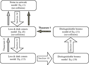
Figure 1: Schematic representation of the considered models of imperfect Boson Sampling with indicated equations where they appear and sections which discuss the models and relations between them. The models used to prove theorems 1 and 2 (section III.2 below) are also indicated. At the bottom of the figure, the two models are for $M\geq N$, beyond the no-collision regime.

III.2 Main results

The main results, proven in the present work in sections VII and VIII, respectively, can be stated as follows.

Theorem 1

Given $0<\delta<1$ and $\varepsilon>0$, the noisy Boson Sampling model of Eq. (1) in the no-collision regime with noise amplitude $\epsilon=\Omega(1)$ can be simulated classically, with success probability at least $1-\delta$, to the error $\varepsilon$ in the total variation distance with computations polynomial $(N,1/\varepsilon,1/\delta)$.

Theorem 1 agrees with one of the conclusions of Ref. KK . On the other hand, we also prove the following.

Theorem 2

The noisy Boson Sampling model of Eq. (1) with noise amplitude $\epsilon=O(1/N)$ is as hard to simulate classically in the no-collision regime as the ideal Boson Sampling.

Our results also indicate that the output distribution of the noisy Boson Sampling of theorem 2 is at a constant total variation distance to that of the ideal Boson Sampling (as suggested in Ref. KK ), for arbitrary $M\geq N$, under two plausible conjectures: (i) the noisy Boson Sampling model and the model of Boson Sampling with partially distinguishable bosons of section VI are at the same average total variation distance from the ideal one and (ii) that a bound of Ref. VS15 on the total variation distance to the ideal Boson Sampling is tight.

Our approach does not resolve if noisy Boson Sampling with the noise amplitude $\epsilon=\omega(1/N)$, intermediate between theorems 1 and 2, can be efficiently simulated classically. The output distribution of such a noisy Boson Sampling has vanishing correlations with that of the ideal Boson Sampling KK . We show that the ratio of the effective total number of “noise clicks” to the total number of bosons vanishes as $N\to\infty$ for noise amplitude $\epsilon=o(1)$ (valid for arbitrary relation between $N$ and $M$), see section VIII. Such noise is therefore similar to that with amplitude $\epsilon=O(1/N)$ by the fact that the dominating contribution to the output probability distribution comes from the quantum many-boson interferences. It is natural then to formulate the following conjecture.

Conjecture 1. The noisy Boson Sampling model of Eq. (1) with the noise amplitude $\epsilon=o(1)$ remains hard to simulate classically.

The proofs of theorems 1 and 2 are limited to the no-collision regime, due to the limited applicability of the methods and results of Refs. VS14 ; R1 ; Brod , used in the proofs. The main technical challenges for extension beyond the no-collision regime are (i) evaluating the averages over the Haar-random network without using the Gaussian approximation (ii) extension of the quantum computational complexity results to many-boson interference beyond the no-collision regime.

Relations with the previous results

Table 1: Reported results on classical hardness/simulatability of imperfect Boson Sampling reformulated for noisy Boson Sampling model of Eq. (1) by using the established equivalence. Here the “necessary” and “sufficient” stand for the necessary and sufficient bounds on $\epsilon$ for classical hardness of noisy Boson Sampling, whereas “classical simulations” stands for sufficient condition for efficient classical simulations. Results apply to no-collision Boson Sampling, those marked with “${\dagger}$” apply also for arbitrary $M\geq N$. Bounds with “$*$” are conjectures (the question mark denotes possible interpretation of the result of Ref. KK ).

	Equivalent bound on noise amplitude $\epsilon$			Bound on error per network element
Reference	Necessary	Sufficient	Classical simulations	Necessary	Sufficient
Ref. KK		$o\left(\frac{1}{N}\right)$, $\left[o\left(\frac{1}{N}\right)^{\dagger}\right]^{*}$	$\Omega(1)$, $\left[\omega\left(\frac{1}{N}\right)^{\dagger}\right]^{*}(?)$
Ref. LP	$O\left(\frac{\log M}{N^{2}}\right)$			$O\left(\frac{1}{N^{2}}\right)$
Ref. Arkhipov		$o\left(\frac{1}{N^{2}}\right)^{\dagger}$			$o\left(\frac{1}{N^{2}\log M}\right)^{\dagger}$
Ref. VS15	$\left[o\left(\frac{1}{N}\right)^{\dagger}\right]^{*}$	$o\left(\frac{1}{N}\right)^{\dagger}$
Ref. Brod		$O\left(\frac{1}{N}\right)$
Refs. R1 ; RSP			$\Omega(1)$
Refs. OB ; PRS			$\left[1-o\left(\frac{1}{\sqrt{N}}\right)\right]^{\dagger}$
Present		$O\left(\frac{1}{N}\right)$, $o(1)^{*}$	$\Omega(1)$		$O\left(\frac{1}{N\log M}\right)$, $o\left(\frac{1}{\log M}\right)^{*}$

Ref. RR mentioned that there may be an equivalence of partial distinguishability to losses of bosons in their effect on Boson Sampling. In this work, this is taken further by establishing actual equivalence of three noise models, the network noise of Refs. LP ; KK , the partial distinguishability of bosons VS14 ; VS15 , and the shuffled bosons model of Ref. Brod , i.e., when losses of bosons are compensated by dark counts of detectors. This equivalence allows for precise comparison of the previous results, reformulated here for the noise amplitude $\epsilon$ of Eq. (1), see table 1 (detailed in the discussion below).

Ref. LP considered a model of noise in unitary network, where two-dimensional unitary matrices $u_{i}$ from a product decomposition of a unitary multi-port network $U=\prod_{i}u_{i}$ Reck94 ; Clem2016 have noisy elements, introduced by the relation $\Phi(u_{i})\Phi(u_{i}^{\dagger})=e^{i\tilde{\epsilon}h}$, where $\Phi$ is a random map representing noise, $\tilde{\epsilon}>0$ is the amplitude of noise, and $h$ is a two-dimensional Hermitian matrix consisting of independent Gaussian random variables with zero average and unit variance. Therefore, the average probability of an error per element is $O(\tilde{\epsilon}^{2})$, whereas in a random unitary network the total variation distance to the ideal Boson Sampling becomes LP

$$\langle\mathcal{D}\rangle_{\Phi,U}=\Omega(\tilde{\epsilon}^{2}N^{2}).$$ (2)

To connect the noise amplitude $\tilde{\epsilon}$ of LP with $\epsilon$ of Eq. (1) note that for a single boson at input the average probability of an error to occur is $O(\tilde{\epsilon}^{2}d)$, where $d$ is the network depth $d=O(\log M)$ AA (i.e., the current necessary number of elementary blocks in the unitary matrix factorisation by $2$-dimensional ones, as in Ref. Reck94 ). On the other hand, in the Gaussian noise model Eq. (1) the average probability of an error is $O(\epsilon)$ (as it is quadratic in the matrix element). We have $\epsilon\sim\tilde{\epsilon}^{2}\log M$ (first established in Ref. Arkhipov ). Therefore, the necessary condition on the average probability of error per network element $\tilde{\epsilon}^{2}=O(1/N^{2})$ LP , for classical hardness of such a noisy Boson Sampling, in our terms reads $\epsilon=O(\log M/N^{2})$.

On the other hand, a sufficient condition on imperfect/noisy unitary matrix $\tilde{U}$ was obtained in Ref. Arkhipov by establishing a bound on the total variation distance

$$\mathcal{D}\leq N||U-\tilde{U}||,$$ (3)

where $||\ldots||$ is the matrix norm. There it was also shown that for the Gaussian noise model of Ref. KK

$$||U-\mathcal{U}||=O(\sqrt{\epsilon}).$$ (4)

By Eqs. (3)-(4) a sufficient condition for a small total variation distance $\mathcal{D}=o(1)$ to the ideal Boson Sampling reads $\epsilon=o(1/N^{2})$ Arkhipov . Theorem 2 reduces the sufficient condition for classical hardness to $\epsilon=O(1/N)$. Therefore, it relaxes also the sufficient condition on the average probability of error per network element from $o(1/(N^{2}\log M))$ (according to the above result of Ref. Arkhipov ) to $O(1/(N\log M))$. Note that this new sufficient bound does not satisfy the necessary one of Ref. LP (the resolution of this apparent contradiction is given below).

Ref. VS15 gives a sufficient bound on boson distinguishability, i.e., on the overlap of internal states of bosons $\xi=1-o(1/N)$, sufficient for the total variation distance to the ideal Boson Sampling to be $\mathcal{D}=o(1)$ for arbitrary $M\geq N$. This condition corresponds to the noise amplitude $\epsilon=o(1/N)$ (under the conjecture that the two models of noise are equivalent, see sections VI.1 and VII), which agrees with the noise stability of Boson Sampling shown in Ref. KK for $\epsilon=o(1/N)$. Moreover, the condition $\epsilon=o(1/N)$ is conjectured in Ref. VS15 to be also necessary for vanishing total variation distance to the ideal Boson Sampling (again, there is an apparent contradiction with the sufficient bound due to theorem 2, $\epsilon=O(1/N)$, see below).

We use the equivalence between the models of imperfections and the results of Ref. Brod to prove theorem 2 stating that noisy Boson Sampling with noise amplitude $\epsilon=O(1/N)$ is as classically hard as the ideal Boson Sampling. Ref. KK (and the above discussed conjecture of Ref. VS15 ) states that such noisy Boson Sampling is at a constant total variation distance from the ideal one. These facts give the resolution of the apparent disagreement between theorem 2 and the necessary bounds of Refs. LP ; KK ; VS15 : closeness to the ideal (noiseless) Boson Sampling is not the only possible reason for classical hardness of noisy Boson Sampling. We can conclude that the necessary bounds on noise/imperfection amplitude derived before by requiring a small total variation distance to the ideal Boson Sampling may be actually not necessary for the classical hardness of noisy/imperfect Boson Sampling. This also makes the analysis of Ref. BSECT irrelevant, since the classical hardness of an imperfect/noisy realisation of Boson Sampling was assumed there to be equivalent to it being at a small total variation distance from the ideal model.

Theorem 1 states efficient classical simulatability of no-collision Boson Sampling on a noisy network with the noise amplitude $\epsilon=\Omega(1)$, additionally to the previously proven classical simulatability for finite partial distinguishability, i.e., finite overlap of internal states of bosons, $\xi=1-\Omega(1)$, R1 , and for losses of bosons proportional to the total number of them RSP , i.e., with the transmission $\eta=1-\Omega(1)$.

In Refs. OB ; PRS it was shown that Boson Sampling on a lossy network with the (maximal) transmission $\eta=o(1/\sqrt{N})$ can be efficiently simulated classically for any $M\geq N$. This bound transforms into an equivalent one on the amplitude of noise in Eq. (1) $\epsilon=1-o(1/\sqrt{N})$. Ref. K1 has shown that lossy Boson Sampling with any finite transmission and stronger dark counts than in the discrete representation of noisy Boson Sampling, derived below in section IV, can be efficiently simulated classically. However, this result does not apply beyond the no-collision regime, since it depends on the usage of boson number unresolving detectors, which are sufficient only in the no-collision regime AA .

Finally, if conjecture 1 of section III.1 on classical hardness of noisy Boson Sampling with the noise with amplitude $\epsilon=o(1)$ is true, this would mean that the average acceptable probability of error per network element has to be just $o(1/\log M)$, i.e., smaller than the inverse of network depth AA .

IV Output probability distribution of noisy Boson Sampling

Let us find the output probability distribution of the noisy Boson Sampling model in the no-collision regime, given by Eq. (1). We fix the input ports to be $k=1,\ldots,N$. Assuming that the matrix $Z$ changes from run to run, let us derive the probability $\langle p^{(\mathcal{U})}(l_{1}\ldots l_{N}|1\ldots N)\rangle$ to detect $N$ input bosons at distinct output ports $l_{1},\ldots,l_{N}$. Denoting by $\mathcal{M}(k_{1}\ldots k_{n}|l_{1}\ldots l_{n})$ the submatrix of a matrix $\mathcal{M}$ on the rows $k_{1},\ldots,k_{n}$ and columns $l_{1},\ldots,l_{n}$, by $\mathrm{per}\mathcal{M}(k_{1}\ldots k_{n}|l_{1}\ldots l_{n})$ the matrix permanent of such a submatrix, and (in this and the next section) by $\langle\ldots\rangle$ the averaging over the noise $Z$, we have

$$\langle p^{(\mathcal{U})}(l_{1}\ldots l_{N}|1\ldots N)\rangle=\left\langle\bigl{|}\mathrm{per}\mathcal{U}(1\ldots N|l_{1}\ldots l_{N})\bigr{|}^{2}\right\rangle$$

$$=\left\langle\Biggl{|}\sum_{n=0}^{N}\epsilon^{\frac{n}{2}}(1-\epsilon)^{\frac{N-n}{2}}\sum_{k_{1}\ldots k_{n}}\sum_{{j_{1}}\ldots{j_{n}}}\mathrm{per}Z(k_{1}\ldots k_{n}|l_{j_{1}}\ldots l_{j_{n}})\mathrm{per}U(k_{n+1}\ldots k_{N}|l_{j_{n+1}}\ldots l_{j_{N}})\Biggr{|}^{2}\right\rangle,$$ (5)

where we partition the set $1,\ldots,N$ twice into two groups of subsets: (i) $k_{1},\ldots,k_{n}$ and $k_{n+1},\ldots,,k_{N}$ and (ii) ${j_{1}},\ldots,{j_{n}}$ and ${j_{n+1}},\ldots,{j_{N}}$ (here and below the notation $\sum_{k_{1}\ldots k_{n}}$ stands for the summation over all subsets, $k_{1},\ldots,k_{n}$, taken from a larger set, in Eq. (IV) from $1,\ldots,N$) and expand the matrix permanent of the sum of two matrices in Eq. (1) using the permanent expansion formula Minc . The averaging over the noise is easily performed within the expansion in Eq. (IV), where we need to consider the averaging of the products of the following type (we use that each output probability involves only a submatrix of $\mathcal{U}$ of size $N$, therefore we are in the applicability of domain of approximation by Eq. (1), see the note below Eq. (1) in section II)

$$\langle\mathrm{per}Z(k_{1}\ldots k_{n}|l_{j_{1}}\ldots l_{j_{n}})\mathrm{per}Z^{*}(k^{\prime}_{1}\ldots k^{\prime}_{m}|l_{j^{\prime}_{1}}\ldots l_{j^{\prime}_{m}})\rangle$$

$$=\sum_{\sigma\in S_{n}}\sum_{\tau\in S_{m}}\left\langle\left[\prod_{\alpha=1}^{n}Z_{k_{\sigma(\alpha)},l_{j_{\alpha}}}\right]\prod_{\beta=1}^{m}Z^{*}_{k^{\prime}_{\tau(\beta)},l_{j_{\beta}^{\prime}}}\right\rangle$$

$$=\frac{\delta_{n,m}}{M^{n}}\sum_{\sigma,\tau\in S_{n}}\prod_{\alpha=1}^{n}\delta_{k_{\sigma(\alpha)},k^{\prime}_{\tau(\alpha)}}\delta_{l_{j_{\alpha}},l_{j^{\prime}_{\alpha}}}$$

$$=\delta_{n,m}\frac{n!}{M^{n}}\prod_{\alpha=1}^{n}\delta_{k_{\alpha},k^{\prime}_{\alpha}}\delta_{l_{j_{\alpha}},l_{j^{\prime}_{\alpha}}},$$ (6)

where we have used that $Z$ is a matrix of i.i.d. Gaussians with $\langle Z_{kl}\rangle=0$ and $\langle|Z_{kl}|^{2}\rangle=1/M$. Inserting the result of Eq. (IV) into Eq. (IV), introducing the binomial distribution

$$B_{n}(x)\equiv\binom{N}{n}x^{n}(1-x)^{N-n}$$ (7)

and rearranging the summations (with $n$ and $N-n$ interchanged) we obtain the output probability of Eq. (IV) as follows

$$\langle p^{(\mathcal{U})}(l_{1}\ldots l_{N}|1\ldots N)\rangle=\sum_{n=0}^{N}B_{n}(1-\epsilon)\frac{(N-n)!}{M^{N-n}}$$

$$\times\binom{N}{n}^{-1}\sum_{{j_{1}}\ldots{j_{n}}}\sum_{k_{1}\ldots k_{n}}p^{(U)}_{q}(l_{j_{1}}\ldots l_{j_{n}}|k_{1}\ldots k_{n}),$$ (8)

where

$$p^{(U)}_{q}(l_{j_{1}}\ldots l_{j_{n}}|k_{1}\ldots k_{n})=\left|\mathrm{per}U(k_{1}\ldots k_{n}|l_{j_{1}}\ldots l_{j_{n}})\right|^{2}.$$ (9)

Eq. (9) gives the probability of $n$ indistinguishable bosons, sent to distinct input ports $k_{1},\ldots,k_{n}$ of the unitary network $U$, to be detected at distinct output ports $l_{j_{1}},\ldots,l_{j_{n}}$ C .

All the factors on the r.h.s. of Eq. (IV) have physical interpretation as some probabilities. The factor $B_{n}(1-\epsilon)$ is the probability that only $n$ of the total $N$ input bosons, from $n$ random input ports, remain indistinguishable during the propagation in the noisy network. These bosons contribute the probability factor

$$\overline{p^{(U)}_{q}}(l_{j_{1}}\ldots l_{j_{n}})\equiv\binom{N}{n}^{-1}\sum_{k_{1}\ldots k_{n}}p^{(U)}_{q}(l_{j_{1}}\ldots l_{j_{n}}|k_{1}\ldots k_{n}).$$ (10)

The rest $N-n$ of the input bosons behave as distinguishable bosons (or classical particles), uniformly randomly populating the output ports, thus contributing the probability factor $(N-n)!/M^{N-n}$. Observe that the Gaussian noise in Boson Sampling is now represented as uniform losses with the transmission $1-\epsilon$ (Eq. (10) is equivalent to that for a Boson Sampling with a lossy input, with only $n$ out of $N$ bosons making to a network), compensated by dark (random) counts of detectors at output ports: there so many (uniformly distributed) dark counts as the lost bosons, so that the total number of detector clicks is equal to the total number of input bosons. The action of noise is therefore similar to the model of shuffled bosons discussed in Ref. Brod (note, however, that the probability distribution of our “dark counts” is different from that of physical dark counts of detectors, see more on this in section V). We will use this equivalence in section VIII to prove theorem 2 of section III.2.

V Extending the Gaussian noise model beyond the no-collision regime

The discrete representation of the Gaussian noise, Eq. (IV) of section IV, allows one to extend the noisy Boson Sampling model of Ref. KK for arbitrary $N,M$, i.e., beyond the usual no-collision regime. Generally speaking, such an extension is not unique. We choose an extension of noise that has a similar effect on the many-boson interference in the general case as the Gaussian noise in the no-collision regime. Since all the factors in Eq. (IV) are interpreted as some probabilities, such an extension can be easily obtained by generalising them and the summation over distinct output ports $l_{j_{1}},\ldots,l_{j_{n}}$ in Eq. (IV) for general $N,M$.

For arbitrary $N,M$ there are multiply occupied output ports, hence, we have a multi-set $l_{1}\leq\ldots\leq l_{N}$. Let us fix the notations for below. We denote by $\mathbf{m}=(m_{1},\ldots,m_{M})$, $|\mathbf{m}|\equiv m_{1}+\ldots+m_{M}=N$, the output configuration corresponding to a multi-set $l_{1}\leq\ldots\leq l_{N}$ (where $m_{l}$ is the total number of bosons in output port $l$), whereas $\mathbf{s}=(s_{1},\ldots,s_{M})$, $|\mathbf{s}|=n$, and $\mathbf{r}=(r_{1},\ldots,r_{M})$, $|\mathbf{r}|=N-n$, will denote the output configurations corresponding, respectively, to the multi-subsets $l_{j_{1}}\leq\ldots\leq l_{j_{n}}$ and $l_{j_{n+1}}\leq\ldots\leq l_{j_{N}}$ of the above multi-set (thus $\mathbf{m}=\mathbf{r}+\mathbf{s}$). We also set $\mathbf{m}!\equiv m_{1}!\ldots m_{M}!$.

First, the probability of an output configuration $\mathbf{r}$ obtained by uniformly randomly distributing $N-n$ distinguishable bosons, or, equivalently PartDist , indistinguishable classical particles over the output ports reads

$$q(\mathbf{r})=\frac{(N-n)!}{\mathbf{r}!M^{N-n}}.$$ (11)

Eq. (11) can be derived as follows. Assume that classical particles are enumerated (i.e., classical and distinguishable), then the probability to get any given output is $1/M^{N-n}$, since each time one chooses one of $M$ ports uniformly randomly. Ignoring the identities of the particles, we obtain for an output configuration $\mathbf{r}$ exactly $(N-n)!/\mathbf{r}!$ distributions of distinguishable classical particles, i.e., the probability in Eq. (11).

Second, the summation over the subsets of distinct output ports $l_{j_{1}}<\ldots<l_{j_{n}}$, (equivalently, over the subindices $1\leq{j_{1}}<\ldots<{j_{n}}\leq N$) in Eq. (IV) must be replaced for general $M\geq N$ by the summation over all sub-configurations $\mathbf{s}\subset\mathbf{m}$ (i.e., $s_{\alpha}\leq m_{\alpha}$ for all $\alpha=1,\ldots,M$), each corresponding to a multi-set of the output ports $l_{j_{1}}\leq\ldots\leq l_{j_{n}}$, to ensure that we do not double count the same output configurations (since different subsets $1\leq{j_{1}}<\ldots<{j_{n}}\leq N$ may correspond to the same output configuration $\mathbf{s}$). There is a mathematical relation between the two types of summations valid for any symmetric function $f(l_{1},\ldots,l_{N})$ (e.g., Ref. Minc )

$$\sum_{{\mathbf{s}\subset\mathbf{m}\atop|\mathbf{s}|=n}}f(l_{1},\ldots,l_{N})=\sum_{{j_{1}}\ldots{j_{n}}}f(l_{1},\ldots,l_{N})\prod_{\alpha=1}^{M}\binom{m_{\alpha}}{s_{\alpha}}^{-1}.$$ (12)

With the above two observations, replacing the output port indices by the corresponding occupations, i.e., $l_{1}\ldots l_{N}$ by $\mathbf{m}$ and $l_{j_{1}}\ldots l_{j_{n}}$ by $\mathbf{s}$, the probability distribution of Eq. (IV) generalised beyond the no-collision regime becomes

$$\langle p^{(\mathcal{U})}(\mathbf{m}|1\!\ldots\!N)\rangle\equiv\sum_{n=0}^{N}B_{n}(1-\epsilon)$$

$$\times\binom{N}{n}^{-1}\sum_{k_{1}\ldots k_{n}}\sum_{{\mathbf{s}\subset\mathbf{m}\atop|\mathbf{s}|=n}}q(\mathbf{r})p^{(U)}_{q}(\mathbf{s}|k_{1}\!\ldots\!k_{n}),$$

here $p^{(U)}(\mathbf{s}|k_{1}\ldots k_{n})$ is the probability for indistinguishable bosons from input ports $k_{1},\ldots,k_{n}$ to be detected in output configuration $\mathbf{s}$ corresponding to multi-set of output ports $l_{j_{1}}\leq\ldots\leq l_{j_{n}}$ C ; Scheel ; AA

$$p^{(U)}_{q}(\mathbf{s}|k_{1}\!\ldots\!k_{n})=\frac{1}{\mathbf{s}!}\left|\mathrm{per}U(k_{1}\ldots k_{n}|l_{j_{1}}\ldots l_{j_{n}})\right|^{2},$$ (14)

generalising that of Eq. (9). One can verify by straightforward calculation with use of the summation identity Minc ,

$$\sum_{|\mathbf{m}|=N}f(l_{1},\ldots,l_{N})=\sum_{l_{1}=1}^{M}\dots\sum_{l_{N}=1}^{M}\frac{\mathbf{m}!}{N!}f(l_{1},\ldots,l_{N}),$$ (15)

valid for any symmetric function $f(l_{1},\ldots,l_{N})$, and unitarity of the network matrix $U$, that the probabilities in Eq. (V) sum to $1$,

$$\sum_{|\mathbf{m}|=N}\langle p^{(\mathcal{U})}(\mathbf{m}|1\ldots N)\rangle=1.$$

The equivalent representation of the Gaussian noise found in section IV, Eq. (IV), and extended here for $M\geq N$, Eq. (V), is the basis for our analysis of the effect of noise on Boson Sampling.

Let us return here to the equivalence of the noisy Boson Sampling model Eq. (V) to that with losses and dark counts of detectors, discussed at the end of section IV. There is some difference between our model of dark counts and the dark counts of independent physical detectors, with each detector following Poisson distribution $p(n)=\frac{\nu^{n}}{n!}e^{-\nu}$, $\nu>0$. The probability of $N-n$ dark counts of physical detectors in an output configuration $\mathbf{r}$ would be in this case given by the distribution

$$\tilde{q}(\mathbf{r})=\frac{\nu^{N-n}}{\mathbf{r}!}e^{-M\nu},$$ (16)

which is different from the probability $q(\mathbf{r})$ of Eq. (11) describing a model of correlated dark counts at output ports. The output distribution in Eq. (V) shows nevertheless equivalence to the shuffled bosons model of Ref. Brod , where the lost bosons are compensated exactly by the dark counts of detectors in uniformly random output ports. Moreover, as we discuss below, there is also an approximate equivalence of the noisy Boson Sampling model to that with partially distinguishable bosons (and no noise).

VI Noise in Boson Sampling and partial distinguishability of bosons

The representation of the Gaussian noise by its action on many-boson interference, discussed in sections IV and V, allows one also to reveal a relation between the effect of noise and that of partial distinguishability of bosons on classical hardness of Boson Sampling. Such a relation will be useful in the proof of classical simulatability of the noisy BosonSamling model (sectionVII).

In the discrete representation of noisy Boson Sampling model, Eq. (V), distinguishable bosons are uniformly randomly distributed at the output ports (equivalent of the correlated dark detector counts) to compensate for the lost indistinguishable bosons. Consider a related imperfect Boson Sampling model, where $N-n$ distinguishable bosons are also sent through a unitary (noiseless) network along with $n$ indistinguishable ones, complementing the input ports to $1,\ldots,N$, with the total number $n$ of the indistinguishable bosons distributed according to the binomial of Eq. (7) with $x=1-\epsilon$. The probability of uniformly randomly distributing $N-n$ particles over the output ports of Eq. (11) must be replaced in this case by the classical probability of the respective output sub-configuration $\mathbf{r}$ of $N-n$ distinguishable bosons (which depends on the absolute values squared of the network matrix elements). We conjecture that replacing in Eq. (V) the uniform probability with a classical probability has no effect on the classical hardness of the output distribution. Indeed, classical probabilities are given by the matrix permanents of doubly-stochastic matrices (with the elements $|U_{kl}|^{2}$), simulated by an efficient classical algorithm JSV . The conjecture is also partially confirmed below: (i) by comparison of our condition on the noise amplitude, obtained under the conjecture in subsection VI.1, with the previously established bounds LP ; Arkhipov and (ii) in section VII, where we find that conditions on classical simulatability of the Boson Sampling with partially distinguishable bosons and that on the noisy Boson Sampling are the same for the same amplitude of respective imperfections.

Before continuing, let us recall the basics of the partial distinguishability theory (see Refs. VS14 ; PartDist ; Ninter for more details). In this theory, bosonic degrees of freedom are partitioned into two types: the operating modes and the internal states. A unitary network performs a unitary transformation $U$ of the operating modes, whereas the internal modes allow to distinguish bosons, at least in principle. Assuming that bosons are in the same pure internal state (i.e., the state over all other degrees of freedom other than the operating modes PartDist ) one obtains the output probability formula of Eq. (14) C ; AA . The usual operating modes of single photons, for example, are the propagating modes of a spatial optical network. Another possibility is to use the temporal operating modes, i.e., the time-bins TbinBS ; TbinBSExp . However, $N$ single photons, usually coming from distinct sources or at different times from a single source, are not in the same internal pure state. Single photon generation is a probabilistic process with all the available to-date sources (see for instance Ref. SPS ), experimentally available single photons are in some mixed states. Assuming that the internal states are not resolved (such resolution only adds network-independent randomness to boson counts), the probability of an output configuration $\mathbf{m}=(m_{1},\ldots,m_{M})$ (corresponding to a multi-set of output ports $l_{1}\leq\ldots\leq l_{N}$) in the general case of partially distinguishable bosons at the input ports $k=1,\ldots,N$ becomes VS14 ; PartDist ; Ninter

$$p^{(U)}_{J}(\mathbf{m}|1\!\ldots\!N)\!=\!\frac{1}{\mathbf{m}!}\sum_{\sigma_{1},\sigma_{2}}\!J(\sigma_{1}\sigma^{-1}_{2})\prod_{k=1}^{N}U^{*}_{\sigma_{1}(k),l_{k}}U_{\sigma_{2}(k),l_{k}},$$ (17)

where the double summation with $\sigma_{1},\sigma_{2}$ runs over the symmetric group $S_{N}$ of $N$ objects. Here a complex-valued (distinguishability) function $J(\sigma)$ depends on the internal state of $N$ bosons $\rho\in H^{\otimes N}$, where $H$ is the internal Hilbert space of single boson, and is defined as follows VS14 ; PartDist

$$J(\sigma)=\mathrm{Tr}\{P_{\sigma}\rho\},$$ (18)

with $P_{\sigma}$ being the unitary operator representation of the symmetric group $S_{N}$ action in the tensor product $H^{\otimes N}$. In the case of completely indistinguishable bosons $J(\sigma)=1$, for all $\sigma\in S_{N}$, we recover from Eqs. (17)-(18) the probability of Eq. (14), whereas for $J(\sigma)=\delta_{\sigma,I}$, with $I$ being the identity permutation (orthogonal internal states), the probability formula for completely distinguishable bosons (or indistinguishable classical particles) VS14 ; PartDist .

The discussion at the beginning of this section can be summarised by replacing the output distribution of Eq. (V) by the following distribution

$$p^{(U)}_{J}(\mathbf{m}|1\ldots N)=\sum_{n=0}^{N}B_{n}(1-\epsilon)\binom{N}{n}^{-1}$$ (19)

$$\times\sum_{k_{1}\ldots k_{n}}\sum_{{\mathbf{s}\subset\mathbf{m}\atop|\mathbf{s}|=n}}p^{(U)}_{q}(\mathbf{s}|k_{1}\!\ldots\!k_{n})p^{(U)}_{cl}(\mathbf{r}|k_{n+1}\ldots k_{N}),$$

here the probability factor (11) in Eq. (V) is replaced by the classical probability of $N-n$ distinguishable bosons, sent at the inputs $k_{n+1},\ldots,k_{N}$, to be detected in the configuration $\mathbf{r}$ of output ports, i.e.,

$$\!\!\!\!\!\!\!p^{(U)}_{cl}(\mathbf{r}|k_{n+1}\!\ldots\!k_{N})\!=\!\frac{1}{\mathbf{r}!}\sum_{\sigma\in S_{N\!-\!n}}\prod_{\alpha=n\!+\!1}^{N}|U_{k_{\sigma(\alpha)},l_{j_{\alpha}}}|^{2}$$

$$=\frac{1}{\mathbf{r}!}\mathrm{per}|U|^{2}(k_{n+1}\!\ldots\!k_{N}|l_{j_{n+1}}\!\ldots\!l_{j_{N}}),$$ (20)

where $l_{j_{n+1}}\leq\ldots\leq l_{j_{N}}$ are the output ports corresponding to $\mathbf{r}$. For instance, in a uniform network $|U_{kl}|=\frac{1}{\sqrt{M}}$ the probabilities of Eqs. (11) and (VI) coincide.

Now, we can introduce a model of partial distinguishability which results precisely in the output distribution of Eq. (19) (another such model is presented in section VII). Consider $N$ single bosons, where boson at input port $k$ is in the following internal state

$$\rho_{k}=(1-\epsilon)|\phi_{0}\rangle\langle\phi_{0}|+\epsilon|\phi_{k}\rangle\langle\phi_{k}|,$$ (21)

where $\langle\phi_{i}|\phi_{j}\rangle=\delta_{i,j}$ for all $i,j\in\{0,1,\ldots,N\}$. Eq. (21) means that with probability $1-\epsilon$ boson $k$ is in the common pure state $|\phi_{0}\rangle$ and with probability $\epsilon$ in a unique ortogonal state $|\phi_{k}\rangle$. The internal state of $N$ such independent bosons reads $\rho=\rho_{1}\otimes\ldots\otimes\rho_{N}$. By Eq. (21) and orthogonality of the specific states $|\phi_{k}\rangle$, the probability to have $n$ indistinguishable single bosons (at randomly chosen input ports) is $B_{n}(1-\epsilon)$, where $B_{n}(x)$ is the binomial distribution (7). The partial distinguishability function is straightforward to obtain from the definition (18). By expanding the tensor product $\rho_{1}\otimes\ldots\otimes\rho_{N}$ using the expression of Eq. (21) and substituting the result into Eq. (18) we get

$$J(\sigma)=\sum_{n=0}^{N}(1-\epsilon)^{n}\epsilon^{N-n}\sum_{k_{1}\ldots k_{n}}\prod_{\alpha=n+1}^{N}\delta_{k_{\sigma(\alpha)},k_{\alpha}}$$

$$=\sum_{n=0}^{N}(1-\epsilon)^{n}\epsilon^{N-n}\sum_{k_{1}\ldots k_{n}}\sum_{\tau\in S_{n}}\delta_{\sigma,\tau\otimes I},$$ (22)

where the two subsets $k_{1},\ldots,k_{n}$ and $k_{n+1},\ldots,k_{N}$ of $1,\ldots,N$ give the contributions from the first and the second terms in Eq. (21), respectively, (the second subset contains only the fixed points of permutation $\sigma$ by orthogonality of the unique states $|\phi_{k}\rangle$, $k=1,\ldots,N$). Thus for each subset $k_{1},\ldots,k_{n}$ the nonzero terms in Eq. (VI) correspond to permutations of the type $\sigma=\tau\otimes I$, with $\tau\in S_{n}$ acting on this subset.

Using the partial distinguishability of Eq. (VI) in the general formula (17) reproduces the result of Eq. (19). Indeed, modifying slightly Eq. (17), by setting $\sigma=\sigma^{-1}_{2}$ and $\sigma_{R}=\sigma_{1}\sigma_{2}^{-1}$, reordering the factors in the product, and using the identity of Eq. (12) we get

$$p^{(U)}_{J}(\mathbf{m}|1\ldots N)=\frac{1}{\mathbf{m}!}\sum_{\sigma_{R},\sigma\in S_{N}}J(\sigma_{R})\prod_{k=1}^{N}U^{*}_{\sigma_{R}(k),l_{\sigma(k)}}U_{k,l_{\sigma(k)}}$$

$$=\frac{1}{\mathbf{m}!}\sum_{n=0}^{N}B_{n}(1-\epsilon)\binom{N}{n}^{-1}\sum_{k_{1}\ldots k_{n}}\sum_{\tau_{R}\in S_{n}}\underbrace{\sum_{\sigma\in S_{N}}}\left[\prod_{\alpha=1}^{n}U^{*}_{k_{\tau_{R}(\alpha)},l_{\sigma(k_{\alpha})}}U_{k_{\alpha},l_{\sigma(k_{\alpha})}}\right]\prod_{\alpha=n+1}^{N}|U_{k_{\alpha},l_{\sigma(k_{\alpha})}}|^{2}$$

$$=\frac{1}{\mathbf{m}!}\sum_{n=0}^{N}B_{n}(1-\epsilon)\binom{N}{n}^{-1}\sum_{k_{1}\ldots k_{n}}\sum_{\tau_{R}\in S_{n}}\underbrace{\sum_{j_{1}\ldots j_{n}}\sum_{\pi\in S_{n}}\sum_{\mu\in S_{N-n}}}\left[\prod_{\alpha=1}^{n}U^{*}_{k_{\tau_{R}(\alpha)},l_{j_{\pi}(\alpha)}}U_{k_{\alpha},l_{j_{\pi}(\alpha)}}\right]\prod_{\alpha=n+1}^{N}|U_{k_{\alpha},l_{j_{\mu(\alpha)}}}|^{2}$$

$$=\frac{1}{\mathbf{m}!}\sum_{n=0}^{N}B_{n}(1-\epsilon)\binom{N}{n}^{-1}\sum_{k_{1}\ldots k_{n}}\sum_{j_{1}\ldots j_{n}}\left[\sum_{\nu\in S_{n}}\prod_{\alpha=1}^{n}U^{*}_{k_{\alpha},l_{j_{\nu(\alpha)}}}\right]\left[\sum_{\pi\in S_{n}}\prod_{\alpha=1}^{n}U_{k_{\alpha},l_{j_{\pi}(\alpha)}}\right]\sum_{\mu\in S_{N-n}}\prod_{\alpha=n+1}^{N}|U_{k_{\alpha},l_{j_{\mu(\alpha)}}}|^{2}$$

$$=\sum_{n=0}^{N}B_{n}(1-\epsilon)\binom{N}{n}^{-1}\sum_{k_{1}\ldots k_{n}}\sum_{j_{1}\ldots j_{n}}\left[\prod_{\alpha=1}^{M}\binom{m_{\alpha}}{s_{\alpha}}^{-1}\right]p^{(U)}_{q}(\mathbf{s}|k_{1}\ldots k_{n})p^{(U)}_{cl}(\mathbf{r}|k_{n+1}\ldots k_{N})$$

$$=\sum_{n=0}^{N}B_{n}(1-\epsilon)\binom{N}{n}^{-1}\sum_{k_{1}\ldots k_{n}}\sum_{{\mathbf{s}\subset\mathbf{m}\atop|\mathbf{s}|=n}}p^{(U)}_{q}(\mathbf{s}|k_{1}\ldots k_{n})p^{(U)}_{cl}(\mathbf{r}|k_{n+1}\ldots k_{N}),$$

where we have taken into account that by Eq. (VI) $\sigma_{R}=\tau_{R}\otimes I$, introduced $\nu=\pi\tau_{R}^{-1}$ to factor the summations over the permutations, and used the underbraces to show the factorisation of permutation $\sigma\in S_{N}$ as follows $\sigma=(\pi\otimes\mu)\rho$ with arbitrary permutations $\pi\in S_{n}$ and $\mu\in S_{N-n}$ and $\rho\in S_{N}/(S_{n}\otimes S_{N-n})$ (i.e., from the factor group) selecting a subset $j_{1},\ldots,j_{n}$ from $1,\ldots,N$.

VI.1 Sufficient condition on noise amplitude for closeness of noisy Boson Sampling and the ideal one

In Ref. VS15 a plausibly tight bound was found for closeness in the total variation distance of the output distribution of imperfect Boson Sampling with partially distinguishable bosons to that of the ideal Boson Sampling. Here we consider the bound in relation to the noisy Boson Sampling model. The bound is as follows. The output probability distribution of Boson Sampling with $N$ partially distinguishable bosons in an internal state given by $J(\sigma)$ (18) (and no other imperfections in the setup) is at most at $(1-d_{J}(N))$-distance in the total variation distance to the ideal Boson Sampling,

$$\mathcal{D}=\frac{1}{2}\sum_{|\mathbf{m}|=N}|p^{(U)}_{q}(\mathbf{m})-p^{(U)}_{J}(\mathbf{m})|\leq 1-d_{J}(N),$$ (23)

where

$$d_{J}(N)=\frac{1}{N!}\sum_{\sigma\in S_{N}}\mathrm{Tr}\{P_{\sigma}\rho^{(int)}\}=\frac{1}{N!}\sum_{\sigma\in S_{N}}J(\sigma).$$ (24)

The bound of Eq. (23) can be easily understood: the quantity $d_{J}(N)$ of Eq. (24) is the magnitude of projection on the subspace of $H^{\otimes N}$ consisting of the completely symmetric internal states (such an internal state corresponds to the completely indistinguishable bosons PartDist ). Indeed, the projection reads

$$\rho^{(S)}=\hat{S}_{N}\rho\hat{S}_{N},\quad\hat{S}_{N}\equiv\frac{1}{N!}\sum_{\sigma\in S_{N}}P_{\sigma},$$ (25)

giving $d_{J}(N)=\mathrm{Tr}\{\rho^{(S)}\}=\mathrm{Tr}\{\hat{S}_{N}\rho\}$ by the fact that $\hat{S}^{2}_{N}=\hat{S}_{N}$. We obtain from Eqs. (VI) and (24)

$$d_{J}(N)=\frac{1}{N!}\sum_{n=0}^{N}\epsilon^{n}(1-\epsilon)^{N-n}\sum_{k_{1}\ldots k_{n}}\sum_{\sigma\in S_{N}}\prod_{\alpha=n+1}^{N}\delta_{k_{\sigma(\alpha)},k_{\alpha}}$$

$$=\frac{1}{N!}\sum_{n=0}^{N}\epsilon^{n}(1-\epsilon)^{N-n}\sum_{k_{1}\ldots k_{n}}\sum_{\sigma\in S_{N-n}}1$$

$$=(1-\epsilon)^{N}\sum_{n=0}^{N}\frac{1}{n!}\left(\frac{\epsilon}{1-\epsilon}\right)^{n}\geq(1-\epsilon)^{N}$$ (26)

(where for small $\epsilon$ the lower bound is also numerically very close to the exact value). Eqs. (23) and (VI.1) tell us that if $\epsilon\leq 1-(1-\varepsilon)^{\frac{1}{N}}=(1+|O(\varepsilon)|)\varepsilon/N$, i.e., for $\varepsilon\ll 1$ if

$$\epsilon\leq\frac{\varepsilon}{N},$$ (27)

is satisfied, the Boson Sampling with partially distinguishable bosons with the distinguishability function of Eq. (VI) is $\varepsilon$-close in the total variation distance to the ideal Boson Sampling. Assuming the equivalence between the two models of imperfections in their effect on the computational complexity of Boson Sampling, Eq. (27) applies also to the noisy Boson Sampling. Note that Eq. (27) agrees with the conclusion of Ref. KK on noise stability of Boson Sampling for noise amplitudes $\epsilon=o(1/N)$. This agreement supports our conjecture on the equivalence of the effect of noise to that of distinguishability on Boson Sampling. However, in section VIII we will show that condition (27) is not necessary for classical hardness of noisy Boson Sampling.

VII Efficient classical simulation of the noisy Boson Sampling with finite noise

In this section we further explore the connection of the noisy Boson Sampling to that with partially distinguishable bosons, discussed in section VI. This connection allows us to prove theorem 1 of section III.2. It should be stressed, that our proof does not depend on the conjectured equivalence of the effect of two models of imperfection on Boson Sampling. The main utility of the above connection is to simplify some technical calculations, that are much easier for the partial distinguishability model than for the noise model, but, as we show, the results apply to the latter model as well. Most of the technical calculations, employed below for the Boson Sampling model with partially distinguishable bosons, have been performed before in Ref. VS14 , in the no-collision regime. Below we consider this regime only and heavily rely on the results of Appendix B of Ref. VS14 . Moreover, at the end of this section, we provide an additional argument supporting the conjectured equivalence of the noisy Boson Sampling model Eq. (V) and that with partially distinguishable bosons Eq. (19) in terms of the classical simulatability.

Let us first derive an equivalent, much simpler, representation of the distinguishability function of Eq. (VI). We will use the indicator function $I_{D_{k_{1},\ldots,k_{n}}}(\sigma)$ of derangements of $k_{1},\ldots,k_{n}$, i.e., the class of permutations of this set not having fixed points (e.g., Ref. Stanley ), and the identities:

$$\sum_{k_{1}\ldots k_{n}}I_{D_{k_{1},\ldots,k_{n}}}(\sigma)=\delta_{C_{1}(\sigma),N-n},$$ (28)

$$\prod_{\alpha=1}^{s}\delta_{k_{\sigma(\alpha)},k_{\alpha}}=\sum_{m=s}^{N}\delta_{C_{1}(\sigma),m}\sum_{k_{s+1}\ldots k_{m}}I_{D_{k_{m+1},\ldots,k_{N}}}(\sigma),$$

where the summation in the first line is over all $s$-dimensional subsets $k_{1},\ldots,k_{n}$ of $1,\ldots,N$, $C_{1}(\sigma)$ is the total number of fixed points of permutation $\sigma$, in the second line $k_{s+1},\ldots,k_{m}$ is the subset of $1,\ldots,N$ consisting of the fixed points of $\sigma$ additional to $k_{1},\ldots,k_{s}$ on the l.h.s..

An equivalent representation of $J(\sigma)$ of Eq. (VI) is obtained by performing summation with use the identities of Eq. (28), we get

$$J(\sigma)=\sum_{s=0}^{N}\epsilon^{s}(1-\epsilon)^{N-s}\sum_{k_{1}\ldots k_{s}}\prod_{\alpha=1}^{s}\delta_{k_{\sigma(\alpha)},k_{\alpha}}$$

$$=\sum_{s=0}^{N}\epsilon^{s}(1-\epsilon)^{N-s}\sum_{k_{1}\ldots k_{s}}\sum_{m=s}^{N}\sum_{k_{s+1}\ldots k_{m}}I_{D_{k_{m+1},\ldots,k_{N}}}(\sigma)$$

$$=\sum_{m=0}^{N}\sum_{k_{1}\ldots k_{m}}\sum_{s=0}^{m}\binom{m}{s}\epsilon^{s}(1-\epsilon)^{N-s}I_{D_{k_{m+1},\ldots,k_{N}}}(\sigma)$$

$$=\sum_{m=0}^{N}\sum_{k_{1}\ldots k_{m}}(1-\epsilon)^{N-m}I_{D_{k_{m+1},\ldots,k_{N}}}(\sigma)$$

$$=(1-\epsilon)^{N-C_{1}(\sigma)},$$

where in the intermediate steps we have introduced the total number ($m$) of fixed points of permutation $\sigma$ and the fixed points themselves $k_{1},\ldots,k_{m}$.

Eq. (VII) means that in the model of Eq. (21) permutation $\sigma$ is weighted according to the number of derangements $N-C_{1}(\sigma)$, thus a permutation with more fixed points $C_{1}(\sigma)$ contributes with a larger weight to the output probability.

There is another input state with partially distinguishable bosons, different from that of Eq. (21), giving the same distinguishability function (VII). This input state consists of bosons in pure internal states $|\psi_{k}\rangle$ with a uniform overlap $\langle\psi_{k}|\psi_{l}\rangle=1-\epsilon$ for $k\neq l$. Precisely this model was used previously R1 ; RSP in the proof of classical simulatability of Boson Sampling with partially distinguishable bosons. This simplifies our task, as we can follow the previous approach. The main step is to consider the following auxiliary version of an imperfect Boson Sampling with partially distinguishable bosons, where many-boson quantum interference is allowed only to some order $R$

$$\tilde{J}(\sigma)=(1-\epsilon)^{N-C_{1}(\sigma)}\theta(C_{1}(\sigma)-N+R),$$

$$\theta(m)=\left\{\begin{array}[]{cc}1,&m\geq 0,\\ 0,&m<0.\end{array}\right.$$ (32)

Now we consider the output probability distributions corresponding to the above two models of partial distinguishability, $J$ of Eq. (VII) and $\tilde{J}$ of Eq. (VII). Boson Sampling with $J$ of Eq. (VII) in the no-collision regime has the output probability distribution given by Eq. (19), which we reproduce here (omitting the input ports $1,\ldots,N$, for simplicity)

$$p(l_{1}\ldots l_{N})=\sum_{n=0}^{N}B_{n}(1-\epsilon)\binom{N}{n}^{-1}$$ (33)

$$\times\sum_{{j_{1}}\ldots{j_{n}}}\sum_{k_{1}\ldots k_{n}}p^{(U)}_{q}(l_{j_{1}}\ldots l_{j_{n}}|k_{1}\ldots k_{n})$$

$$\times p^{(U)}_{cl}(l_{j_{n+1}}\ldots l_{j_{N}}|k_{n+1}\ldots k_{N}).$$

To obtain the output probability distribution for $\tilde{J}$ of Eq. (VII), we rewrite the $\tilde{J}$-function as the second line of Eq. (VI) with the right hand side multiplied by $\theta(C_{1}(\sigma)-N+R)$, i.e.,

$$\widetilde{J}(\sigma)\!=\!\sum_{n=0}^{N}(1\!-\!\epsilon)^{n}\epsilon^{N-n}\!\sum_{k_{1}\ldots k_{n}}\sum_{\tau\in S_{n}}\theta(C_{1}(\tau)-n+R)\delta_{\sigma,\tau\otimes I},$$ (34)

where we have used that $C_{1}(\sigma)=N-n+C_{1}(\tau)$ for $\sigma=\tau\otimes I$. Comparing with Eq. (VI) we obtain from Eq. (33) the probability distribution for $\tilde{J}$ of Eqs. (VII) and (34), which we will call the auxiliary Boson Sampling model with partially distinguishable bosons,

$$\tilde{p}(l_{1}\ldots l_{N})=\sum_{n=0}^{N}B_{n}(1-\epsilon)\binom{N}{n}^{-1}$$ (35)

$$\times\sum_{{j_{1}}\ldots{j_{n}}}\sum_{k_{1}\ldots k_{n}}\tilde{p}^{(U)}_{q}(l_{j_{1}}\ldots l_{j_{n}}|k_{1}\ldots k_{n}),$$

$$\times p^{(U)}_{cl}(l_{j_{n+1}}\ldots l_{j_{N}}|k_{n+1}\ldots k_{N})$$

where now

$$\tilde{p}^{(U)}(l_{j_{1}}\ldots l_{j_{n}}|k_{1}\ldots k_{n})$$ (36)

$$=\sum_{\sigma_{1},\sigma_{2}}\theta(C_{1}(\sigma_{1}\sigma^{-1}_{2})-n+R)\prod_{\alpha=1}^{n}U^{*}_{k_{\sigma_{1}(\alpha)},l_{j_{\alpha}}}U_{k_{\sigma_{2}(\alpha)},l_{j_{\alpha}}},$$

with the double summation over $\sigma_{1,2}\in S_{n}$. The $\theta$-function in Eq. (36) cuts-off the many-boson interferences at the order $R$, since there must be at least $n-R$ fixed points of $\tau$ (see for more details Ref. Ninter ).

Note that by the results of sections IV and VI, if in Eqs. (33) and (35) we replace the classical probability factors by their averages in a random network $U$, i.e., $\langle p^{(U)}_{cl}(l_{j_{n+1}}\ldots l_{j_{N}}|k_{n+1}\ldots k_{N})\rangle=\frac{(N-n)!}{M^{N-n}}$ (in the no-collision regime), we obtain the noisy Boson Sampling model of Eq. (IV) and, what we will call below, the auxiliary noisy Boson Sampling model.

It is known that, on average in a random network $U$, the output probability distributions of Eqs. (33) and (35) can be made arbitrarily close in the total variation distance for any finite distinguishability $\xi=1-\epsilon$ by selecting such a $R=O(1)$ and that the auxiliary Boson Sampling model of Eq. (35) can be efficiently simulated classically for $R=O(1)$ R1 . In our proof of efficient classical simulatability of the noisy Boson Sampling model, however, we will need some technical details of derivation of an upper bound on the total variation distance between two distributions of Boson Sampling with different partial distinguishability functions VS14 . These details allow us to easily extend the proof of efficient classical simulatability to the noisy Boson Sampling model as well.

Consider the variation distance $\mathcal{D}$ between the output distributions of Eqs. (33) and (35) over the no-collision outputs $l_{1}<\ldots<l_{N}$ (the outputs with collisions can be neglected, since their contribution is vanishing as $O(N^{2}/M)$ AA ; Bbirthday ). If we average $\mathcal{D}$ over the random unitary $U$, where we can use the approximation of its elements by i.i.d. Gaussians AA , we obtain

$$\langle\mathcal{D}\rangle=\frac{1}{2}\sum_{l_{1}\ldots l_{N}}\langle|p(l_{1}\ldots l_{N})-\tilde{p}(l_{1}\ldots l_{N})|\rangle$$

$$\leq\frac{1}{2}\sum_{l_{1}\ldots l_{N}}\sqrt{\langle\left(p(l_{1}\ldots l_{N})-\tilde{p}(l_{1}\ldots l_{N})\right)^{2}\rangle}$$

$$=\frac{1}{2}\sum_{l_{1}\ldots l_{N}}\frac{N!}{M^{N}}\left[\frac{1}{N!}\sum_{\sigma\in S_{N}}\left[J(\sigma)-\tilde{J}(\sigma)\right]^{2}\chi(C_{1}(\sigma))\right]^{\frac{1}{2}}$$

$$=\frac{1}{2}\left[\frac{1}{N!}\sum_{\sigma\in S_{N}}\left[J(\sigma)-\tilde{J}(\sigma)\right]^{2}\chi(C_{1}(\sigma))\right]^{\frac{1}{2}},$$ (37)

where we have used that for any real random variable $X$ $\langle|X|\rangle\leq\sqrt{\langle X^{2}\rangle}$ , that the average probability is equal to the inverse of the number of no-collision output configurations (approximated in the no-collision regime by ${M^{N}}/{N!}$) and that the average of the squared difference reads

$$\langle\left(p(l_{1}\ldots l_{N})-\tilde{p}(l_{1}\ldots l_{N})\right)^{2}\rangle$$

$$=\frac{N!}{M^{2N}}\sum_{\sigma\in S_{N}}\left[J(\sigma)-\tilde{J}(\sigma)\right]^{2}\chi(C_{1}(\sigma)),$$ (38)

with

$$\chi(n)\equiv\sum_{\tau\in S_{n}}2^{C_{1}(\tau)}=n!\sum_{k=0}^{n}\frac{1}{k!}.$$ (39)

The derivation of Eq. (VII) just repeats that of Appendix B in Ref. VS14 , where one only has to replace the distinguishability function of the ideal Boson Sampling $\tilde{J}(\sigma)=1$ by that of the model (VII).

The right hand side of Eq. (VII) can be easily estimated. Introducing the variable $s\equiv C_{1}(\sigma)$ and using the expressions for $J$ and $\tilde{J}$, Eqs. (VII) and (VII), we obtain

$$\frac{1}{N!}\sum_{\sigma\in S_{N}}\left[J(\sigma)-\tilde{J}(\sigma)\right]^{2}\chi(C_{1}(\sigma))$$

$$=\frac{1}{N!}\sum_{s=0}^{N-R-1}\chi(s)(1-\epsilon)^{2[N-s]}\sum_{\sigma\in S_{N}}\delta_{C_{1}(\sigma),s}$$

$$<\sum_{s=0}^{N-R-1}(1-\epsilon)^{2[N-s]}\left(1+\frac{e}{(N-s+1)!}\right)$$

$$<\left(1+\frac{e}{(R+2)!}\right)\sum_{s=0}^{N-R-1}(1-\epsilon)^{2[N-s]}$$

$$<\left(1+\frac{e}{(R+2)!}\right)\frac{(1-\epsilon)^{2[R+1]}}{1-(1-\epsilon)^{2}},$$ (40)

where we use $\chi(s)<s!e$ and a bound on the total number of derangements with $N-s$ elements Stanley

$$\sum_{\sigma\in S_{N}}\delta_{C_{1}(\sigma),s}=\frac{N!}{s!}\sum_{i=0}^{N-s}\frac{(-1)^{i}}{i!},$$

following from

$$\sum_{i=0}^{N-s}\frac{(-1)^{i}}{i!}<\left\{\begin{array}[]{cc}e^{-1},&N-s=odd,\\ e^{-1}+\frac{1}{(N-s+1)!},&N-s=even\end{array}\right.$$

(the sum of two consecutive terms is always positive in the odd case, the even case is reduced to the odd one by adding the term with $i=N-s+1$). Substitution of the expression in Eq. (VII) into Eq. (VII) gives an upper bound for the average total variation distance in the no-collision regime (up to a vanishing term $O(N^{2}/M)$) between the distributions in Eqs. (33) and (35)

$$\langle\mathcal{D}\rangle<\frac{1}{2}\left(1+\frac{e}{(R+2)!}\right)^{\frac{1}{2}}\frac{(1-\epsilon)^{R+1}}{\sqrt{\epsilon(2-\epsilon)}}.$$ (41)

We obtain that for any $\varepsilon>0$ and the cut-off order of the many-boson interference $R$ given by

$$R=\frac{\ln\left(\frac{\sqrt{2}}{\varepsilon\sqrt{\epsilon}}\right)}{\ln\left(\frac{1}{1-\epsilon}\right)}$$ (42)

the average variation distance (41) between the probability distributions of Eqs. (33) and (35) is bounded as $\langle\mathcal{D}\rangle<\varepsilon/2$. It is easy to see that for any given error $\varepsilon$, to have $R=O(1)$, as $N\to\infty$, requires that $\epsilon$ is bounded from below away from zero, i.e., $\epsilon=\Omega(1)$.

The remaining step is to show that the upper bound given in Eq. (41) on the total variation distance between the output distributions of Boson Sampling model with partially distinguishable bosons, Eq. (33), and the auxiliary model admitting efficient classical simulations, (35), remains valid if we make in these two models the same transformation: replace the classical probability factors in the respective output distributions by the average value in a random network $U$. As is noted above, on such a replacement the model of Eq. (33) becomes the noisy Boson Sampling model of Eq. (IV), whereas the other model obviously continues to allow for efficient classical simulations (in this case, there is no need to simulate the classical probabilities). To the above goal, we need some facts established previously VS14 on the main ingredient of the upper bound – the variance of the difference in respective probabilities. The variance is given by Eq. (VII), since in the no-collision regime the average probability is uniform over the output ports, independently of the distinguishability function VS14 . Replacing the classical probability factor by its average in the output distributions can only decrease the variance of the difference, since the classical factors in different terms in the respective output probability distributions, i.e., in the sums in Eqs. (33) and (35), contain independent random variables, due to mutual independence of elements of a random unitary matrix in the no-collision regime AA . Therefore, we have proven that Eq. (41) gives the required bound on the total variation distance between noisy Boson Sampling model of Eqs. (IV) or (1) and an auxiliary model that can be efficiently simulated classically.

The classical simulatability result can be formulated as follows R1 : the number of classical computations required to simulate the noisy Boson Sampling model Eq. (33) to a given error $\varepsilon$ and with the probability of success at least $1-\delta$ for any $\delta>0$ is a polynomial function of $(N,1/\varepsilon,1/\delta)$ for $\epsilon=\Omega(1)$. Hence, we have proven theorem 1 of section III. An explicit algorithm for classical simulations of Boson Sampling with partially distinguishable bosons of Eq. (VII) is the same as in Refs. R1 ; RSP (see the comment in the paragraph above Eq. (VII)).

Now let us examine by how much the variance of the difference in Eq. (VII) decreases after replacing the classical probability factors in Eqs. (33) and (35) by the average values. The change of the variance in the Gaussian approximation comes from the fourth-order moments $\langle|U_{kl}|^{4}\rangle=2/M^{2}$ (appearing when averaging a squared classical probability factor) being replaced by $(\langle|U_{kl}|^{2}\rangle)^{2}=1/M^{2}$. But the fourth-order moments that are being replaced are weighted at least by $\epsilon^{2}$, since they come from the noise contribution to output distribution of noisy Boson Sampling, where each term is weighted at least by $\epsilon$ (the variance is quadratic function in the probability and different matrix elements are mutually independent random variables in the no-collision regime). The decrease in the relative variance is therefore on the order $O(\epsilon^{2})$. This very small difference in the variance for small amplitude of imperfection, when switching between the noisy Boson Sampling model and that with partially distinguishable bosons, supports the conjecture of section VI on their equivalence in terms of classical hardness.

VIII How many “noise clicks” in noisy Boson Sampling?

Let us return to the output probability distribution of Eq. (V), i.e., the equivalent representation of the noisy Boson Sampling model. It replaces the continuous model of noise by an equivalent one with discrete “noise clicks” (i.e., lost bosons compensated by random detector counts). Consider now the noisy Boson Sampling model with $N$ input bosons, but with the number of “noise clicks” bounded by $R-1$. Given $\varepsilon\ll 1$, what number of clicks $R=R(N,\varepsilon)$ is sufficient to approximate the output probability distribution of a given noisy Boson Sampling (V) to the total variation distance $\mathcal{D}\leq\varepsilon$? The question is answered below and the answer allows to prove theorem 2 of section III by using the results of Ref. Brod .

The probability distribution of the noisy Boson Sampling model with the total number of “noise clicks” bounded by $R-1$ is obtained by imposing a cut-off on the summation index $N-R+1\leq n\leq N$ in Eq. (V) and rescaling (here we use $\langle\ldots\rangle$ to denote averaging over the noise $Z$, as in sections IV and V)

$$\langle p^{(\mathcal{U})}_{R}(\mathbf{m}|1\!\ldots\!N)\rangle=C_{R}\sum_{n=N-R+1}^{N}B_{n}(1-\epsilon)$$

$$\times\binom{N}{n}^{-1}\sum_{k_{1}\ldots k_{n}}\sum_{{\mathbf{s}\subset\mathbf{m}\atop|\mathbf{s}|=n}}q(\mathbf{r})p^{(U)}_{q}(\mathbf{s}|k_{1}\!\ldots\!k_{n}),$$

where $C_{R}=\sum B_{n}(1-\epsilon)$ for $N-R+1\leq n\leq N$. We get the following bound on the total variation distance between models of Eq. (V) and (VIII)

$$\mathcal{D}=\frac{1}{2}\sum_{\mathbf{m}}|\langle p^{(\mathcal{U})}(\mathbf{m}|1\!\ldots\!N)\rangle-\langle p^{(\mathcal{U})}_{R}(\mathbf{m}|1\!\ldots\!N)\rangle|$$

$$\leq\frac{1}{2}\left(\left[\frac{1}{C_{R}}-1\right]\sum_{n=N-R+1}^{N}B_{n}(1-\epsilon)+\sum_{n=0}^{N-R}B_{n}(1-\epsilon)\right)$$

$$=\sum_{n=0}^{N-R}B_{n}(1-\epsilon)=\sum_{s=R}^{N}B_{s}(\epsilon),$$ (44)

where to perform summation over $\mathbf{m}$ we have used that the terms in Eq. (VIII) (as well as in Eq. (V)) are positive and represent certain probabilities.

One immediate consequence of Eq. (VIII) is that for noise amplitude $\epsilon=O(1/N)$ and any given small error $\varepsilon$ taking $R=O(1)$ is sufficient to bound the total variation distance as required, $\mathcal{D}\leq\varepsilon$. Recall that for $\epsilon=O(1/N)$ the binomial distribution $B(\epsilon)$ is approximated by the Poisson distribution with the expected number of clicks $\langle R\rangle=\epsilon N=O(1)$, thus bounding the number of clicks by $R$, such that $R>\langle R\rangle$, is sufficient to approximate the distribution (i.e., make the tail in Eq. (VIII) arbitrarily small). Below this is formally proven with the use of Hoeffding’s bound Hoeffding .

Hoeffding’s bound (see theorem 1 in Ref. Hoeffding ), applied here for the partial sum of the Binomial distribution represented as $N$ i.i.d. trials $x_{i}\in\{0,1\}$, where $x_{i}=1$ with probability $\epsilon$, states that for $\epsilon<R/N<1$

$$\sum_{s=R}^{N}B_{s}(\epsilon)=\mathrm{Prob}\left(\sum_{i=1}^{N}x_{i}\geq R\right)$$

$$\leq\left(\frac{N\epsilon}{R}\right)^{R}\left(\frac{1-\epsilon}{1-R/N}\right)^{N-R}.$$

We conclude that if there is such $R$ satisfying

$$\left(\frac{N\epsilon}{R}\right)^{R}\left(\frac{1-\epsilon}{1-R/N}\right)^{N-R}\leq\varepsilon,\quad R>\epsilon N,$$ (46)

then $\mathcal{D}\leq\varepsilon$ as required. Consider the second factor in the first inequality in Eq. (46), setting $X\equiv(R/N-\epsilon)/(1-\epsilon)$ we obtain

$$\left(\frac{1-\epsilon}{1-R/N}\right)^{N-R}=\exp\{-(N-R)\ln(1-X)\}$$

$$\leq\exp\left\{\frac{(N-R)X}{1-X}\right\}=\exp\left\{\frac{(N-R)(R/N-\epsilon)}{1-R/N}\right\}$$

$$=\exp\{R-N\epsilon\},$$

where we have used that $-\ln(1-X)\leq X/(1-X)$ (here $0<X<1$, under the second condition in Eq. (46)). Then, Eq. (46) follows from the following simpler one

$$\left(\frac{R}{e\epsilon N}\right)^{R}\geq\frac{e^{-\epsilon N}}{\varepsilon},\quad R>\epsilon N,$$ (47)

which can be satisfied for $\epsilon=O(1/N)$ by choosing $R=O(1)$.

The existence of a finite bound $R=O(1)$ on the total number of “noise clicks” resulting in arbitrary closeness of the reduced model Eq. (VIII) in the total variation distance to the noisy Boson Sampling model Eq. (V), and the equivalence of the noisy Boson Sampling model (with bounded “noise clicks”) to that of the shuffled bosons model of imperfect Boson Sampling (boson losses compensated by detector dark counts) with a finite number of losses and dark counts allows us to use the results of Ref. Brod on the classical hardness of such a shuffled bosons model (in the no-collision regime). We get that in the no-collision regime the noisy Boson Sampling with the noise amplitude $\epsilon=O(1/N)$ is as hard as the ideal Boson Sampling for classical simulations. Hence, we have proven theorem 2 of section III.

In Ref. KK it was suggested that for $O(1/N)$-noise the noisy Boson Sampling model of Eq. (1) must be at a finite total variation distance from the ideal one. The same is implied also by Eqs. (23)-(27) of section VI under the conjectured equivalence of the noisy Boson Sampling Eq. (V) and that with partially distinguishable bosons Eq. (19), if the bound in Eq. (23) is tight for the closeness to the ideal Boson Sampling, as suggested in Ref. VS15 . Nevertheless, a finite total variation distance from the ideal Boson Sampling for such noise does not allow, by theorem 2, an efficient classical simulation of the respective noisy Boson Sampling model.

Finally, from section VII and Ref. KK , we know that for finite noise $\epsilon=\Omega(1)$ the noisy Boson Sampling of Eq. (1) can be efficiently simulated classically. Consider now the intermediate noise amplitude $\epsilon=o(1)$. It was shown that the correlation between the noisy and noiseless outcomes of Boson Sampling tends to zero for $\epsilon=\omega(1/N)$ KK . In this case by Eq. (46) $R$ is unbounded and the above proof fails. However, when also $\epsilon=o(1)$ (i.e., vanishing noise amplitude), we can satisfy Eq. (47), as $N\to\infty$, e.g., with $R=2\epsilon N$. Thus in this case the relative effective number of “noise clicks” $R/N$ (the relative effect of noise on $N$-boson quantum interference) is vanishing, similar as in the classically hard case $\epsilon=O(1/N)$. In view of this fact we conjecture that no efficient classical simulation is possible for any small noise amplitude $\epsilon=o(1)$.

IX Conclusion

We have found two physically realistic models of imperfections, the partial distinguishability of bosons and the boson losses compensated by dark counts of detectors, which lead to the Gaussian noise model in Boson Sampling introduced and studied previously in Ref. KK . This enables us to precisely compare previous results on sufficient and necessary conditions for classical hardness of noisy/imperfect realisations of Boson Sampling and present a unified picture of the effect of noise. We find that noisy Boson Sampling with a finite amount of noise, i.e., with the noise amplitude $\epsilon=\Omega(1)$ as $N\to\infty$ allows for efficient classical simulations, which confirms the previous result of Ref. KK . We also prove that noisy Boson Sampling with noise amplitude scaling inversely with the total number of bosons $\epsilon=O(1/N)$ retains classical hardness, though, by Ref. KK , confirmed by our results, its output distribution is far from the ideal Boson Sampling, as it is at a constant total variation distance from the latter. This means that closeness to the ideal Boson Sampling is not the only possible cause of classical hardness of an imperfect (i.e., experimental) realisation, meaning that some of the necessary conditions known in the literature, derived under the requirement of a small such total variation distance, are not actually necessary for classical hardness of a noisy/imperfect physical realisation.

The above facts have strong implications for experimental efforts to demonstrate quantum advantage with Boson Sampling. First of all, our results significantly reduce the previous sufficient condition on the average probability of error (due to noise) in network elements, e.g., beam-splitters, such that an experimental Boson Sampling with $N$ bosons on a $M$-dimensional noisy network remains still classically hard to simulate, from previous $o(1/(N^{2}\log M))$ Arkhipov to $O(1/(N\log M))$, corresponding to the sufficient bound on noise amplitude $\epsilon=O(1/N)$. However, our results also reveal that the latter may not be necessary for classical hardness. By analysis of the physical effect of noise on many-body quantum interference in Boson Sampling, we are driven to the conjecture that any small noise, i.e., with vanishing amplitude $\epsilon=o(1)$ is sufficient for classical hardness of the output distribution, since the ratio of the effective total number of “noise clicks” (lost boson compensated by dark counts of detectors) to the number of bosons $N$ vanishes as $N\to\infty$. This conjecture implies that the efficient classical simulatability threshold lies at $\epsilon=\Omega(1)$ (finite noise). If true, this fact would further reduce the sufficient condition on the average probability of error in network elements from the proven here $O(1/(N\log M))$ to just $o(1/\log M)$, i.e., the error in an elementary block of network should decrease faster than the inverse of network depth.

Moreover, an extension of the Gaussian noise model beyond the usual no-collision regime has been proposed in the present work. At least some of our conclusions, such as the analysis leading to the conjecture above, are valid for general $M\geq N$, beyond the no-collision regime. However, due to technical reasons (we use previous results with restricted validity) the proven results on the computational complexity apply to the no-collision regime only. Efficient classical algorithms due to imperfections in experimental setup exist also for Boson Sampling in arbitrary regime $M\geq N$ K1 ; OB ; PRS . All of these results do not contradict the conjecture that a finite noise amplitude is the threshold of classical simulations of noisy no-collision Boson Sampling. However, this does not imply that this threshold is the same for no-collision and beyond the no-collision regimes of Boson Sampling. New results in this direction indicate strong dependence of sensitivity of Boson Sampling to noise on the ratio between the total number of bosons and network size NEW .

X Acknowledgements

The author was supported by the National Council for Scientific and Technological Development (CNPq) of Brazil, grant 304129/2015-1 and by the São Paulo Research Foundation (FAPESP), grant 2018/24664-9.

References

- (1) J. Preskill, arXiv:1203.5813.
- (2) P. Kaye, R. Laflamme, and M. Mosca, An introduction to quantum computing (Oxford University Press, 2007).
- (3) S. Aaronson and A. Arkhipov, Theory of Computing 9, 143 (2013).
- (4) T. Morimae, K. Fujii, and J. F. Fitzsimons. Phys. Rev. Lett., 112, 130502 (2014).
- (5) M. Bremner, R. Jozsa, and D. Shepherd. Proc. Roy. Soc. Ser. A, 467 459 (2011).
- (6) G. Kalai, Notices of the AMS, 63, 508 (2016).
- (7) A. P. Lund, A. Laing, S. Rahimi-Keshari, T. Rudolph, J. L. O’Brien, and T. C. Ralph, Phys. Rev. Lett. 113, 100502 (2014).
- (8) S. Aaronson and A. Arkhipov, Quant. Inform. & Computation 14, 1383 (2014).
- (9) E. R. Caianiello, Nuovo Cimento, 10, 1634 (1953); Combinatorics and Renormalization in Quantum Field Theory, Frontiers in Physics, Lecture Note Series (W. A. Benjamin, Reading, MA, 1973).
- (10) S. Scheel, arXiv:quant-ph/0406127 (2004).
- (11) H. Minc, Permanents, Encyclopedia of Mathematics and Its Applications, Vol. 6 (Addison-Wesley Publ. Co., Reading, Mass., 1978).
- (12) L. G. Valiant, Theoretical Coput. Sci., 8, 189 (1979).
- (13) S. Aaronson, Proc. Roy. Soc. London A, 467, 3393 (2011).
- (14) M. Jerrum, A. Sinclair, and E. Vigoda, Journal of the ACM 51, 671 (2004).
- (15) H. Ryser, Combinatorial Mathematics, Carus Mathematical Monograph No. 14. (Wiley, 1963).
- (16) D. G. Glynn, Eur. J. of Combinatorics 31, 1887 (2010).
- (17) A. Arkhipov and G. Kuperberg, Geometry & Topology Monographs 18, 1 (2012).
- (18) E. Knill, R. Laflamme, and G. J. Millburn, Nature 409, 46 (2001).
- (19) M. A. Broome, A. Fedrizzi, S. Rahimi-Keshari, J. Dove, S. Aaronson, T. C. Ralph, and A. G. White, Science 339, 794 (2013);
- (20) J. B. Spring, B. J. Metcalf, P. C. Humphreys, W. S. Kolthammer, X.-M. Jin, M. Barbieri, A. Datta, N. Thomas-Peter, N. K. Langford, D. Kundys, J. C. Gates, B. J. Smith, P. G. R. Smith, and I. A. Walmsley, Science, 339, 798 (2013).
- (21) M. Tillmann, B. Dakić, R. Heilmann, S. Nolte, A. Szameit, and P. Walther, Nature Photonics, 7, 540 (2013).
- (22) A. Crespi, R. Osellame, R. Ramponi, D. J. Brod, E. F. Galvão, N. Spagnolo, C. Vitelli, E. Maiorino, P. Mataloni, and F. Sciarrino, Nature Photonics, 7, 545 (2013).
- (23) M. Bentivegna et al, Sci. Adv. 1, e1400255 (2015).
- (24) K. R. Motes, A. Gilchrist, J. P. Dowling, and P. P. Rohde, Phys. Rev. Lett. 113, 120501 (2014).
- (25) Y. He et al, Phys. Rev. Lett. 118, 190501 (2017).
- (26) J. C. Loredo, M. A. Broome, P. Hilaire, O. Gazzano, I. Sagnes, A. Lemaitre, M. P. Almeida, P. Senellart, and A. G. White, Phys. Rev. Lett. 118, 130503 (2017).
- (27) H. Wang et al, Phys. Rev. Lett. 120, 230502 (2018).
- (28) H.-S. Zhong et al, Phys. Rev. Lett. 121, 250505 (2018).
- (29) C. Shen, Z. Zhang, and L.-M. Duan, Phys. Rev. Lett. 112, 050504 (2014).
- (30) B. Peropadre, G. G. Guerreschi, J. Huh, and A. Aspuru-Guzik Phys. Rev. Lett. 117, 140505 (2016).
- (31) S. Goldstein, S. Korenblit, Y. Bendor, H. You, M. R. Geller, and N. Katz, Phys. Rev. B 95, 020502(R) (2017).
- (32) A. Deshpande, B. Fefferman, M. C. Tran, M. Foss-Feig and A. V. Gorshkov, Phys. Rev. Lett. 121, 030501 (2018).
- (33) B. Peropadre, J. Huk and C. Sabín, Sci. Reps 8, 3751 (2018).
- (34) A. Neville, C. Sparrow, R. Clifford, E. Johnston, P. M. Birchall, A. Montanaro, A. Laing, Nature Physics 13, 1153 (2017).
- (35) P. Clifford, and R. Clifford, arXiv:1706.01260 (2017).
- (36) G. Kalai and G. Kindler, arXiv:1409.3093 [quant-ph].
- (37) S. Rahimi-Keshari, T. C. Ralph, and C. M. Caves, Phys. Rev. X 6, 021039 (2016).
- (38) J. J. Renema, A. Menssen, W. R. Clements, G. Triginer, W. S. Kolthammer, and I. A. Walmsley, Phys. Rev. Lett. 120, 220502 (2018).
- (39) M. Oszmaniec and D. J Brod, New J. Phys. 20, 092002 (2018).
- (40) R. García-Patrón, J. J. Renema, and V. S. Shchesnovich, arXiv:1712.10037 [quant-ph].
- (41) J. J. Renema, V. S. Shchesnovich, and R. García-Patrón, arXiv:1809.01953 [quant-ph].
- (42) A. Leverrier and R. García-Patrón, Quant. Inf. & Computation 15, 0489 (2015).
- (43) A. Arkhipov, Phys. Rev. A 92, 062326 (2015).
- (44) V. S. Shchesnovich, Phys. Rev. A 89, 022333 (2014).
- (45) V. S. Shchesnovich, Phys. Rev. A 91, 063842 (2015).
- (46) S. Aaronson and D. J. Brod, Phys. Rev. A 93, 012335 (2016).
- (47) P. P. Rohde and T. C. Ralph, Phys. Rev. A 85, 022332 (2012).
- (48) A. E. Moylett and P. S. Turner, Phys. Rev. A 97, 062329 (2018).
- (49) V. S. Shchesnovich, Phys. Rev. A 91, 013844 (2015).
- (50) M. Reck, A. Zeilinger, H. J. Bernstein, and P. Bertani, Phys. Rev. Lett. 73, 58 (1994).
- (51) W. R. Clements, P. C. Humphreys, B. J. Metcalf, W. S Kolthammer, I. A. Walmsley, Optica 3, 1460 (2016).
- (52) P. P. Rohde, K. R. Motes, P. A. Knott, and W. J. Munro, arXiv:1401.2199 [quant-ph].
- (53) V. S. Shchesnovich and M. E. O. Bezerra, Phys. Rev. A 98, 033805 (2018).
- (54) Single-Photon Generation and Detection, Volume 45: Physics and Applications (Experimental Methods in the Physical Sciences), eds. A. Migdall, S. V. Polyakov, J. Fan, and J. C. Bienfang (Academic Press; first edition, 2013).
- (55) R. P. Stanley, Enumerative Combinatorics, 2nd ed., Vol. 1 (Cambridge University Press, 2011).
- (56) W. Hoeffding, J. of the Amer. Stat. Assoc. 58, 13 (1963).
- (57) V. S. Shchesnovich, arXiv:1905.11458 [quant-ph].