Sounding stellar cycles with $Kepler$ – III. Comparative analysis of chromospheric, photometric and asteroseismic variability

Abstract

By combining ground-based spectrographic observations of variability in the chromospheric emission from Sun-like stars with the variability seen in their eigenmode frequencies, it is possible to relate the changes observed at the surfaces of these stars to the changes taking place in the interior. By further comparing this variability to changes in the relative flux from the stars, one can obtain an expression for how these activity indicators relate to the energy output from the stars. Such studies become very pertinent when the variability can be related to stellar cycles as they can then be used to improve our understanding of the solar cycle and its effect on the energy output from the Sun.

Here we present observations of chromospheric emission in 20 Sun-like stars obtained over the course of the nominal 4-year $Kepler$ mission. Even though 4 years is too short to detect stellar equivalents of the 11-year solar cycle, observations from the $Kepler$ mission can still be used to analyse the variability of the different activity indicators thereby obtaining information of the physical mechanism generating the variability. The analysis reveals no strong correlation between the different activity indicators, except in very few cases. We suggest that this is due to the sparse sampling of our ground-based observations on the one hand and that we are likely not tracing cyclic variability on the other hand. We also discuss how to improve the situation.

1 Introduction

Our Sun shows variability on a number of time scales, where the most pronounced are: the 5-minute p-mode oscillations, the 25-30 days rotational modulation and the 11-year solar cycle (Shapiro et al., 2017). While we have witnessed significant progress in our understanding of the first two phenomena over the last decades, our knowledge of the 11-year solar cycle is still deficient. Especially, our understanding of the long-term modulation of the amplitude of the 11-year solar cycle, where the occurrence of so-called grand minima, like the 17th century Maunder Minimum, constitute a huge challenge (Eddy, 1976). This challenge can be met by making better observations and better models of the Sun and by comparing these to observations and models of other stars (Schrijver & Zwaan, 2008).

Most of the important information we have of the 11-year solar cycle comes from either direct observations of sunspots or from observations of standing oscillations inside the Sun through helioseismology (Christensen-Dalsgaard, 2002; Gizon, 2004). With helioseismology we have learned about the differential rotation pattern of the Sun’s deep interior and about the meridional circulation in the Sun’s convection zone.

For other Sun-like stars (stars with masses and radii similar to the Sun), we have so far mainly obtained information of their magnetic cycles through observations of the temporal evolution of the emission in the Ca ii $H$ and $K$ lines as has been done from the Mount Wilson and Lowell observatories (Baliunas et al., 1995; Wright, 2005). Expectations where therefore high, when the $Kepler$ mission was launched on 7 March 2009. Though the nominal mission lifetime was only 3.5 years, there was in principle nothing that would prevent the mission to be operational for 10+ years, or so we thought. A 10+ years mission would have allowed us not only to detect stellar cycles in a large number of Sun-like stars, it would also have allowed us to use asteroseismology to sound the effect these cycles would have on the deep interior or vice versa. This information could be used to test and improve the models we have for the 11-year solar cycle.

In 2009 we therefore started the Sounding stellar cycles with Kepler program, where we made dual observations of 20 carefully selected Sun-like stars from both the Nordic Optical Telescope (NOT) and $Kepler$. We have earlier presented the strategy behind this program (Karoff et al., 2009, Paper I) and the first results from the measurements of chromospheric emission (Karoff et al., 2013, Paper II). Here we present the full set of measurements made over the course of the $Kepler$ mission from early 2010 to late 2014.

As $Kepler$ was only able to point to the Cygnus field for 4 years, studies of rotation of Sun-like stars experienced more progress than studies of stellar cycles of Sun-like stars. From early on in the mission, surface rotation was identified in a large number of, mainly active, stars (McQuillan et al., 2013; Nielsen et al., 2013; McQuillan et al., 2014; García et al., 2014; Balona & Abedigamba, 2016; Ceillier et al., 2017) and there were even indications of differential rotation (Reinhold et al., 2013; Bonanno et al., 2014; Reinhold & Gizon, 2015; Balona et al., 2016; Karoff et al., 2018; Benomar et al., 2018; Bazot et al., 2018), though the possibility to accurately extract differential rotation from photometry has been called into question (Aigrain et al., 2015; Basri, 2018). The main result of these measurements was that the observations agreed nicely with the theory, especially for the behaviour of differential rotation (Reinhold et al., 2013). The new observations did however, also indicate that stars with a relative main sequence age older than the Sun lose angular momentum slower than generally believed by stellar evolution theory (van Saders et al., 2016). Though this result has received some criticism, mainly focusing on selection bias and underestimation of the age uncertainties (Barnes et al., 2016), the result has later been confirmed by another independent study (dos Santos et al., 2016). Lately, a number of theoretical explanations for the small angular momentum loss of old solar-type stars have also emerged (Metcalfe et al., 2016; Brandenburg et al., 2017; Metcalfe & van Saders, 2017; Judge et al., 2017).

Based on asteroseismic analysis of observations from the CoRoT satellite, there were early claims of stellar cycles as short as 120 days (García et al., 2010). We now know that $F$-type stars slightly hotter than the Sun, with very thin outer convective zones, tend to show irregular variability with characteristic times scales of a few hundred days and not bona fide cycles (Mathur et al., 2013, 2014; Ferreira Lopes et al., 2015; Régulo et al., 2016). Great care should thus be taken when claiming the detection of any cycles with only 4 years of $Kepler$ observations. It is however, very interesting to compare the variability in such different activity indicators, as it can teach us something about the physical mechanisms responsible for generating the variability (Salabert et al., 2016; Mehrabi et al., 2017). Especially, it is interesting to compare magnetic activity indicators originating from the surface to indicators originating from the interior. It is therefore very fortunate that a number of recent studies have been able to use asteroseismology to trace magnetic variability (Kiefer et al., 2017; Salabert et al., 2018; Santos et al., 2018).

As $Kepler$ was designed for exoplanet detection, the photometry is not suited for identifying stellar activity cycles or the effect of stellar activity. The main reason for this is that the mean level of the photometry is normalised by the calibration method every three months. A solution to this was found by Montet et al. (2017), who employed the so-called full-frame images for reconstruction of the photometric long-term variability. They used these measurements to show a transition from spot-dominated to faculae-dominated variability for rotation periods between 15 and 25 days. Another solution was found by Reinhold et al. (2017), who used the variability rather than the intensity to search for stellar cycles in active solar-type stars. Both studies suffered from the short lifetime of the $Kepler$ mission and were thus not able to identify bona fide stellar cycle variability in any of their targets.

The issue with the short lifetime of the $Kepler$ mission was however, not a problem for the high metallicity Sun-like star KIC 8006161. This star was not only part of our NOT program, it was also observed as part of the Mount Wilson HK project (Baliunas et al., 1995) and the California Planet Search program (Wright, 2005). We were thus able to reconstruct a time series of the chromospheric activity measurements dating back to the mid-nineties (with even a few data points in the late seventies and early eighties) that allowed us to measure a bona fide cycle period of $7.41\pm 1.16$ year. As the rising phase of the last cycle was covered by observations from the $Kepler$ mission, this allowed us to compare the realisation of the magnetic activity in different activity indicators related to the chromosphere, photosphere and interior. The relation between these indicators agreed very nicely with theoretical predictions for this high metallicity star, indicating that the cycle in KIC 8006161 does indeed have the same nature as the solar cycle (Karoff et al., 2018).

This study continues the work in Paper I and Paper II. In Paper I we presented the idea behind the Sounding stellar cycles with Kepler program and discussed the strategy for selecting targets. In Paper II we presented the first measurements of chromospheric emission and analysed the dependency between the mean values of these measurements and fundamental stellar parameters obtained from asteroseismology. At the time of the submission and publication, we expected that $Kepler$ would continue the observations in the Cygnus field for 10+ years. Shortly after the publication of Paper II the second reaction wheel failed and the Cygnus field was abandoned. As the idea from the beginning of the program was that we would only make simultaneous observations with the NOT as long as $Kepler$ was operational, we thus also interrupted our NOT program – meaning that we stopped submitting proposals. In this study we thus present 4 years of simultaneous observations of magnetic activity related variability in our 20 target stars.

The main scope of this study is to present the measurements of chromospheric variability from the NOT made simultaneously with the observations by $Kepler$. In order to evaluate the information content in the measurements we also compare our measurements of chromospheric activity variability with asteroseismic measurements (Santos et al., 2018) and photometric measurements (Montet et al., 2017).

Though we did interrupt our NOT program when the second reaction wheel on $Kepler$ failed, we have continued working on a solution for multidecadal observations of the 20 targets, with a dedicated spectrograph installed at the Hertzsprung Stellar Observations Network Group (SONG) telescope at Teide Observatory (Grundahl et al., 2017). We will provide a brief overview of this idea and discuss the lesson learned from our NOT program with respect to S/N, sampling and observation time span.

2 Observations

The spectrographic observations are described in Paper II. They were obtained with the high-resolution FIbre-fed Echelle Spectrograph (FIES) mounted on the NOT (Frandsen & Lindberg, 2000). The target list is provided in Table 1. Most stars were observed for 3 epochs per year in 2010, 2011, 2012 and 2013 (12 epochs in total). The low-resolution fibre (R=25,000) was used for the observations. The spectra were obtained with 7-minute exposures resulting in a S/N above 100 at the blue end of the spectrum for the faintest starts.

The spectra were reduced as described in Paper II using FIEStool.

Table 1: Target list for the sounding stellar cycles with Kepler programme. We also list the Kepler magnitude and $B-V$ values from Høg et al. (2000) and [Fe/H] from Bruntt et al. (2012). The uncertainty on [Fe/H] is 0.06 dex.

KIC ID	$\alpha$ (2000)	$\delta$ (2000)	$k_{p}$	$B-V$	[Fe/H]	$\sigma S$	$\sigma I$ (ppm)	$\sigma(\delta\nu)$ ($\mu$Hz)
01435467	19:28:19.84	37:03:35.3	8.9	0.47$\pm$0.02	-0.01	0.011	634	0.24
02837475	19:10:11.62	38:04:55.9	8.4	0.43$\pm$0.02	-0.02	0.018	617	0.34
03733735	19:09:01.92	38:53:59.6	8.4	0.41$\pm$0.02	-0.04	0.007	1057	–
04914923	19:16:34.88	40:02:50.1	9.4	0.62$\pm$0.03	0.17	0.015	658	0.07
06116048	19:17:46.34	41:24:36.6	8.4	0.57$\pm$0.01	-0.24	0.013	1919	0.11
06603624	19:24:11.18	42:03:09.7	9.0	0.76$\pm$0.03	0.28	0.018	843	0.04
06933899	19:06:58.34	42:26:08.2	9.6	0.59$\pm$0.04	0.02	0.019	736	0.059
07206837	19:35:03.72	42:44:16.5	9.7	0.46$\pm$0.06	0.14	0.020	1354	0.227
08006161	18:44:35.14	43:49:59.9	7.3	0.87$\pm$0.01	0.34	0.018	1941	0.276
08379927	19:46:41.28	44:20:54.7	6.9	0.58$\pm$0.01		0.009	1316	0.161
08694723	19:35:50.58	44:52:49.8	8.8	0.48$\pm$0.02	-0.59	0.014	1741	0.116
09098294	19:40:21.20	45:29:20.9	9.7	0.68$\pm$0.08	-0.13	0.017	1246	0.071
09139151	18:56:21.26	45:30:53.1	9.1	0.52$\pm$0.03	0.11	0.013	1100	0.124
09139163	18:56:22.12	45:30:25.2	8.3	0.49$\pm$0.01	0.15	0.009	1198	0.287
10124866	18:58:03.46	47:11:29.9	7.9	0.57$\pm$0.02	-0.30	0.015	756	–
10454113	18:56:36.62	47:39:23.0	8.6	0.52$\pm$0.02	-0.06	0.009	1151	0.221
11244118	19:27:20.48	48:57:12.1	9.7	0.78$\pm$0.05	0.35	0.016	1312	–
11253226	19:43:39.62	48:55:44.2	8.4	0.39$\pm$0.02	-0.08	0.011	1307	0.225
12009504	19:17:45.80	50:28:48.2	9.3	0.55$\pm$0.03	-0.09	0.012	952	0.138
12258514	19:26:22.06	50:59:14.0	8.0	0.59$\pm$0.01	0.04	0.012	1025	0.093

3 Analysis

The most common activity indicator utilising the Ca ii $H$ and $K$ lines is the so-called $S$ index (Duncan et al., 1991):

$$S=\alpha\cdot\frac{H+K}{R+V}$$ (1)

where $H$ and $K$ are the recorded counts in 1.09 Å full-width at half-maximum triangular bandpasses centred on the Ca ii $H$ and $K$ lines at 396.8 and 393.4 nm, respectively. $V$ and $R$ are two 20 Å wide reference bandpasses centred on 390.1 and 400.1 nm, respectively, while $\alpha$ is a normalisation constant.

The normalisation constant ($\alpha$) can be obtained by measuring a number of stars that were part of the Mount Wilson HK project (Duncan et al., 1991). The calibration does not have to be linear (Isaacson & Fischer, 2010). This approach was however, not followed in Paper II as there was only one star in common between the Mount Wilson HK project and our targets. Instead the excess flux $\Delta\mathcal{F}_{\rm Ca}$ was used as the activity indicator. The excess flux is defined as the surface flux arising from magnetic sources, which is calculated as the flux in the Ca ii $H$ and $K$ lines, subtracting the photospheric flux and the so-called basal flux.

In Karoff et al. (2018) we however, identified 21 stars that were observed by both the California Planet Search program (Wright, 2005; Isaacson & Fischer, 2010) and by some of our programs at the NOT (including both the targets in Paper I and Paper II). These stars were used by Karoff et al. (2018) to calculate a linear transformation between the instrumental $S$ indices measured with the NOT and the $S$ indices measured as part of the California Planet Search program. In order to minimise numerical effects in the calculation of the S indices, all spectra from the NOT and Keck telescope were reanalysed using the same code. The uncertainties of the NOT measurements were obtained using nights with multiple observations to obtain the following relation between the uncertainty of the mean value of the chromospheric activity measured that night and S/N: $\sigma=0.011/\sqrt{\rm S/N}$. An additional flat noise term of 0.002 was added in quadrature (Lovis et al., 2011).

Our calibrated $S$ indices can be used to calculate the excess flux (Rutten, 1984):

$$\mathcal{F}_{\textup{1\text{\AA}}}=10^{-14}S\cdot C_{\rm cf}T_{\rm eff}^{4},$$ (2)

where $C_{\rm cf}$ is the conversion factor given in (Middelkoop, 1982):

$$\mathrm{log}~{}C_{cf}=0.25(B-V)^{3}-1.33(B-V)^{2}+0.43(B-V)+0.24$$ (3)

A number of asteroseismic estimates are available for the effective temperatures, but we recommend the effective temperatures provided in Creevey et al. (2017)

Our calibrated $S$ indices can also be used to calculate the so-called $R^{\prime}_{\rm HK}$ activity indicator, defined as:

$$R^{\prime}_{\rm HK}=R_{\rm HK}-R_{\rm phot},$$ (4)

where $R_{\rm phot}$ is the photospheric contribution to the indicator, which can be calculated using the $B-V$ colour index (Noyes et al., 1984):

$$\mathrm{log}~{}R_{\rm phot}=-4.898+1.918(B-V)^{2}-2.893(B-V)^{3}$$ (5)

and $R_{\rm HK}$ is calculated based on the $S$ indices and the conversion factor given above:

$$R_{\rm HK}=1.34\cdot 10^{-4}C_{cf}S$$ (6)

After various tests we decided to use the $S$ index as the activity indicator. Generally, the results are not significantly affected depending on if the $S$ index or $R^{\prime}_{\rm HK}$ is used as the activity indicator. The reason for this is that our 20 targets span a rather small range in effective temperature. Also, the focus of this study is the temporal variability of individual stars, so the calibration is a minor issue.

4 Results

The Sun shows a strong direct correlation between chromospheric activity, photometric flux and eigenmode frequencies (see Karoff et al., 2018, and reference herein). The reason for this is that changes in all three parameters are caused by magnetic flux tubes rising up through the Sun. In the outermost regions of the near surface convection zone they change the turbulent velocity affecting the eigen frequencies (Dziembowski & Goode, 2004, 2005), in the photosphere they lead to dark sunspots and bright faculae and in the chromosphere they lead to plages (see Solanki et al., 2013, for a recent review). For KIC 8006161 we were able to measure a similar effect for the rising phase of the cycle that started in 2010. We therefore search for similar correlations for the remaining 19 targets. This is done by comparing our measurements of chromospheric emission to the relative flux of the stars measured in the FFI with the method by Montet et al. (2017) with a method similar to what was done for KIC 8006161 by Karoff et al. (2018). In this work, we include a larger region to search for suitable reference targets, encompassing 125 pixels from the observed image of the star on the detector, including its bleed trail, rather than 125 pixels from the stellar centroid. We note that for three targets, KIC 2837475, 6116048, and 10124866, faint background stars overlap with the PSF of the target star, which, if variable, may affect the photometry at the ppm level. The measurements of chromospheric emission is also compared to the eigenmode frequencies presented in Santos et al. (2018). We use the frequency shifts calculated as the mean of the 5 central orders of the radial and dipolar modes (see Santos et al., 2018, for detailed description of this). We present the comparison in Fig. 1. Three stars, KIC 3733735, KIC 10124866 and KIC 11244118 were not included in the analysis by Santos et al. (2018). The comparison between the chromospheric emission and the relative flux of these stars is presented in Fig. 2.

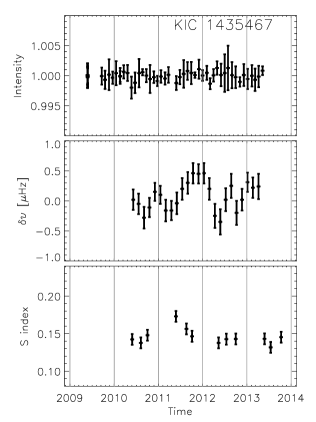
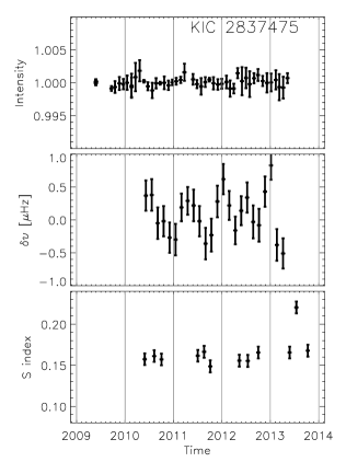
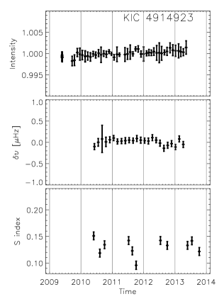
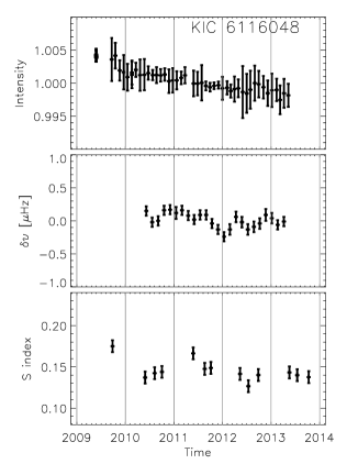
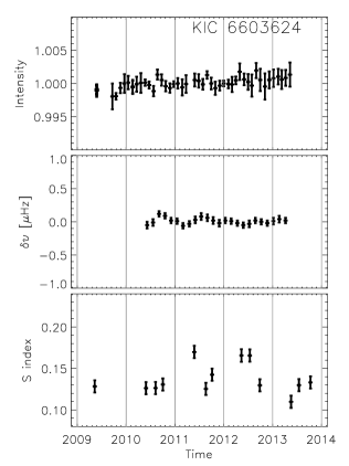
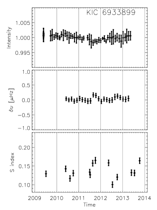
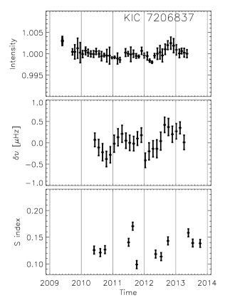
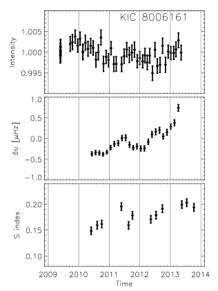
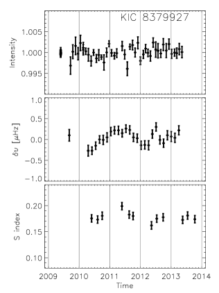
Figure 1: Comparison of chromospheric activity, photometric flux and eigenmode frequencies shifts for the 17 stars with measured eigenmode frequencies in Santos et al. (2018). Tables with the measured parameters are provided in the supplementary material.

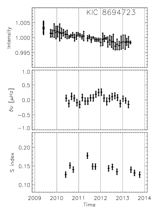
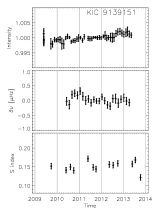
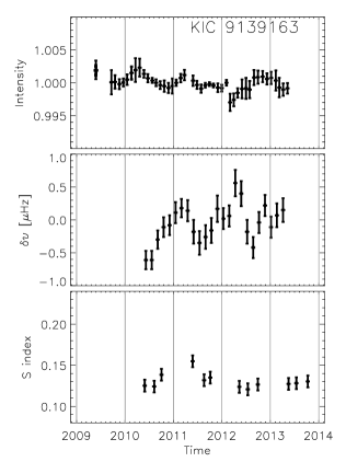
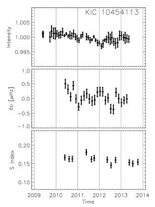
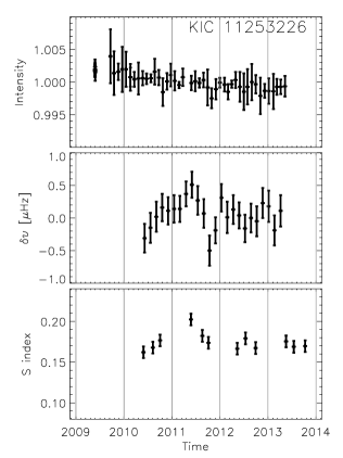
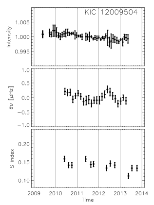
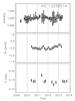
Figure 1: continued

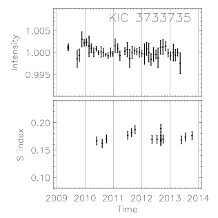
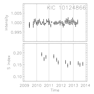
Figure 2: Comparison of chromospheric activity and photometric flux for the 3 stars without measured eigenmode frequencies in Santos et al. (2018). Tables with the measured parameters are provided in the supplementary material.

Based on the results presented in Figs. 1 & 2 we have calculated the standard deviations of each time series. These are provided in Table 1 and in Figs. 3–5 we show the correlation between these standard deviations of the different activity indicators.

We have also calculated the correlation between the chromospheric emission and the eigenmode frequencies (Fig. 6) and between the chromospheric emission and the relative flux (Fig. 7).

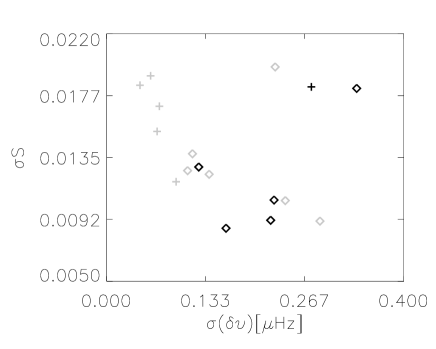
Figure 3: Relation between the standard deviation of the eigenmode frequencies $\sigma(\delta\nu)$ and the chromospheric emission $\sigma S$. Gray make stars with a $S$ index less than 0.15. Crosses mark G-type dwarfs and diamonds mark F-type dwarfs. The spectral type classification has been made based on the effective temperatures.

Figure 4: Relation between the standard deviation of the relative flux $\sigma I$ and the chromospheric emission $\sigma S$. Symbols as in Fig. 3.

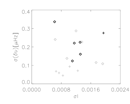
Figure 5: Relation between the standard deviation of the relative flux $\sigma I$ and the eigenmode frequencies $\sigma(\delta\nu)$. Symbols as in Fig. 3.

Figure 6: Correlation between the eigenmode frequencies shifts and the chromospheric emission as a function of the mean value of the chromospheric emission. Crosses mark G-type dwarfs and diamonds mark F-type dwarfs.

Figure 7: Correlation between the relative flux and the chromospheric emission as a function of the mean value of the chromospheric emission. Symbols as in Fig. 6.

We did test all results using $R^{\prime}_{\rm HK}$ instead of the $S$ index and no significant differences were found.

5 Discussions

So far KIC 8006161 is the only star observed by $Kepler$ that is known to show a bona fide cycle comparable to the 11-year solar cycle (see Karoff et al., 2018, for a detailed analysis of this star). In our analysis it is also the only star to show a correlation above the 95% significance level between the variability in the chromospheric emission, the eigenmode frequency shifts and the relative flux.

KIC 10124866 shows a very weak correlation between the chromospheric emission and the relative flux, but the correlation is not above the 95% significance level. No other star shows correlations between the different activity indicators that are above the 95% significance level.

KIC 8379927 shows a nice correlation between the variability in the chromospheric emission and the eigenmode frequencies, but the significance is only 61%. This star is known to be a spectroscopic binary with a $1743.3\pm 2.5$ day period (Griffin, 2007). KIC 8379927 was flagged by Santos et al. (2018) as one of the stars that showed evidence of activity-related frequency shifts. Though the significance is very low, we do agree with this interpretation, that between 2010 and early 2012 KIC 8379927 shows a continuous rise and fall in the frequency shifts that is also seen in the chromospheric emission. It is however, not clearly seen in the relative flux, though the measurements in 2011 seem to show larger than average scatter. It is still too early to conclude if the variability we see in KIC 8379927 is related to a stellar cycle. Looking at the combined frequency shifts and chromospheric emission, there could be hints of a 2-year periodic variability, with maxima in mid-2009, mid-2011 and early/mid-2013. The time-series are however, too short to make any claims about the significance of such periodic variability.

According to Creevey et al. (2017) KIC 8379927 is a Sun-like star with a radius of 1.105 M_⊙, mass of 1.08 M_⊙ and age of 1.65 Gyr. According to García et al. (2014) the star has a rotation period of $16.99\pm 1.35$ days. KIC 8379927 is in other words likely a very Sun-like star and we would therefore expect any periodic variability to be longer than 2 years (Böhm-Vitense, 2007). This however, assumes a large mass difference between the two binary components.

Recently, there has been a number of claims of a biennial cycle in the Sun (Fletcher et al., 2010; Broomhall et al., 2012; Simoniello et al., 2012, 2013). What we are seeing in KIC 8379927 could thus be the manifestation of a second dynamo (Fletcher et al., 2010) comparable to the biennial cycle in the Sun. A number of other G-type dwarfs, like HD 190406, HD 78366 and HD 114710, also show such a secondary biennial cycles (Baliunas et al., 1995; Oláh et al., 2016). Unlike the variability seen in the F-type dwarfs, these secondary biennial cycles seen in the more Sun-like G-type dwarfs could be true polarity reversing solar-like activity cycles (Jeffers et al., 2018). More observations are however, needed before we can make any solid claims. Zeeman-Doppler imaging would be especially useful here, as it can be used to evaluate if we see a polarity flip.

In general the comparison of the standard deviation of the different activity indicators does not show any correlation (Figs. 3–5). In fact there might be hints of an inverse correlation between the standard deviation of the frequency shifts and the chromospheric emission for stars with $S$ indices with a standard deviation less than 0.0177 (Fig. 3). The correlation does not seem to be related to any effective temperature or metallicity effects. As no good explanation for such an inverse correlation exists, this may simply be due to noise.

In Fig. 4 we see an inverse relation between the standard deviation of the relative flux $\sigma I$ and the chromospheric emission $\sigma S$ for the stars with mean chromospheric emission larger than 0.15. This behaviour could be explained by a scenario where stars slightly more active than the Sun goes from being spot dominated to being faculae dominated and in this transition $\sigma I$ decreases with increasing chromospheric activity. Such a inverse relation would not show up for the inactive stars as they would be expected to have a more constant spot-to-faculae ratio throughout the cycle. This means that any spot darkening is balanced out by faculae brightening. The chromospheric emission is however, not affected by this phenomenon.

Alternately, the inverse relation between $\sigma I$ and $\sigma S$ could be explained by shifts in the distributions of active regions, where the area covered by spots increases, but the area covered by plage becomes more spatially homogeneous. These sorts of patterns are seen in more active stars (Radick et al., 2018).

If lack of correlations for the inactive stars is due to a missing degeneracy of the signals form spots and faculae then the problem could be solved by using multi-band photometry, since due to their different temperatures, faculae and spots cannot successfully cancel each other out at all wavelengths.

We do note that we were able in Paper II to see a correlation between the mean value of the excess flux and both the rotation period and age.

We further investigated if the correlation between the different activity indicators depends on the absolute level of the chromospheric emission (Figs 6 & 7). Again, no correlation was found. It is not unlikely that the missing correlation is due to the sparse sampling of the measurements of the chromospheric emission and the fact that the relative flux measurements have to be interpolated for this comparison. In other words, even though we do not see any strong correlation between the different activity indicators, it is not the same as claiming that they are not there.

A correlation between the $R^{\prime}_{\rm HK}$ calibration and metallicity has been noted by Saar (2006), Jenkins et al. (2008) and Saar & Testa (2012). Indicating that metallicity suppress the measured $R^{\prime}_{\rm HK}$ values. We searched for such a correlation between metallicity and the other measured parameters, but did not find any. Again, this could be due to our limited sample size, but also that our stars span a narrow range in effective temperature.

In general, the main conclusion from our work on sounding stellar cycles with Kepler is that we need a longer time baseline for the observations. In the most optimal case this means following the 20 targets in our sample and maybe even more stars indefinitely. We did not find such an approach feasible by submitting new observing proposals to the NOT every semester. Instead we have installed an eShell spectrograph system from Shelyak Instruments at the Hertzsprung SONG telescope at Teide Observatory and are at the moment testing if it can be used, with minor modifications, to measure chromospheric activity in our targets. If these test turn out to be successful, we will have the option to monitor the variability of the chromospheric emission in these stars for as long as SONG is operational. We note that the main spectrograph at SONG is optimised for measuring accurate radial velocities with the use of a iodine cell and is therefore optimised for the wave lengths covered by the main iodine lines (4900-6200 Å). This means that the Ca ii $H$ and $K$ lines do not even fall on the detector.

At SONG we would try to follow an observing strategy that comes closer to the observing strategy used in the Mount Wilson project, where the targets were observed weekly, when visible, than the observing strategy we have used, where the targets were only observed three times per semester. We propose to follow such a strategy, even though it would result in fewer observed targets. There are two main reasons for such a prioritisation. Firstly, as we argue that the missing correlation between the different activity indicators in this study is due to the sparse sampling (and resulting interpolation), a higher sampling cadence should result in higher correlations between the different activity indicators and therefore also more reliable measurements. Secondly, a higher sampling rate would allow a robust mean and standard deviation of the amplitude of the rotational modulation to be calculated. Thirdly, as shown in Karoff et al. (2018), it is possible to use seasonal measured rotation rates to see indications of surface differential rotation caused by active regions at different latitudes. This is however, only possible if sufficient observations are available each semester for determining the rotation period.

Based on our experience with our NOT program, we recommend that the S/N should be not much less that 100 at the blue part of the spectrum in order to be able to obtain reliable activity measurements.

It is our aim that the new spectrograph for measuring stellar activity with SONG should be fully ready for science observations when NASA’s Transiting Exoplanet Survey Satellite (TESS) will start new observations of the $Kepler$ field. This will allow us to test if a denser sampling will lead to a better correlation between the different activity indicators. Apart from this, TESS will provide us with asteroseismic measurements of the fundamental stellar parameters of the stars in which activity cycles have been observed from the Mount Wilson and Lowell observations and will therefore constitute a nice continuation of our sounding stellar cycles with Kepler program. This is especially true if TESS was extended beyond the nominal mission, which would allow the Kepler field to be revisited each summer.

6 Conclusions

We present four years of observations of emission in the Ca ii $H$ and $K$ lines in 20 Sun-like stars. The observations were undertaken simultaneously with observations by the $Kepler$ mission. This has allowed us to analyse the relation between cycle-induced changes on the surface and in the interior in the metal rich Sun-like star KIC 8006161 as seen in the chromospheric emission, in the eigenmode frequencies and in the relative flux (Karoff et al., 2018).

The comparison for the different activity indicators for the remaining 19 stars does however, not show the same agreement as seen for KIC 8006161. We suggest that this is mainly due to two effects. Firstly, the sparse sampling of our spectrographic observations make it difficult to compare with the photometric $Kepler$ observations and secondly, due to the failure of $Kepler^{\prime}s$ reaction wheels, we only have 4 years of observations available, which is not sufficient to detect an activity cycle similar to the 11-year solar cycle. We are therefore trying to set up multidecadal observations of the 20 stars with a new dedicated spectrograph at the SONG telescope.

References

- Aigrain et al. (2015) Aigrain, S., Llama, J., Ceillier, T., et al. 2015, MNRAS, 450, 3211
- Baliunas et al. (1995) Baliunas, S. L., Donahue, R. A., Soon, W. H., et al. 1995, ApJ, 438, 269
- Balona & Abedigamba (2016) Balona, L. A., & Abedigamba, O. P. 2016, MNRAS, 461, 497
- Balona et al. (2016) Balona, L. A., Švanda, M., & Karlický, M. 2016, MNRAS, 463, 1740
- Barnes et al. (2016) Barnes, S. A., Spada, F., & Weingrill, J. 2016, Astronomische Nachrichten, 337, 810
- Basri (2018) Basri, G. 2018, ApJ, 865, 142
- Bazot et al. (2018) Bazot, M., Nielsen, M. B., Mary, D., et al. 2018, arXiv:1810.08630
- Benomar et al. (2018) Benomar, O., Bazot, M., Nielsen, M. B., et al. 2018, Science, 361, 1231
- Böhm-Vitense (2007) Böhm-Vitense, E. 2007, ApJ, 657, 486
- Bonanno et al. (2014) Bonanno, A., Fröhlich, H.-E., Karoff, C., et al. 2014, A&A, 569, A113
- Brandenburg et al. (2017) Brandenburg, A., Mathur, S., & Metcalfe, T. S. 2017, ApJ, 845, 79
- Broomhall et al. (2012) Broomhall, A.-M., Chaplin, W. J., Elsworth, Y., & Simoniello, R. 2012, MNRAS, 420, 1405
- Bruntt et al. (2012) Bruntt, H., Basu, S., Smalley, B., et al. 2012, MNRAS, 423, 122
- Christensen-Dalsgaard (2002) Christensen-Dalsgaard, J. 2002, Reviews of Modern Physics, 74, 1073
- Ceillier et al. (2017) Ceillier, T., Tayar, J., Mathur, S., et al. 2017, A&A, 605, A111
- Creevey et al. (2017) Creevey, O. L., Metcalfe, T. S., Schultheis, M., et al. 2017, A&A, 601, A67
- Dziembowski & Goode (2005) Dziembowski, W. A., & Goode, P. R. 2005, ApJ, 625, 548
- Dziembowski & Goode (2004) Dziembowski, W. A., & Goode, P. R. 2004, ApJ, 600, 464
- dos Santos et al. (2016) dos Santos, L. A., Meléndez, J., do Nascimento, J.-D., et al. 2016, A&A, 592, A156
- Duncan et al. (1991) Duncan, D. K., Vaughan, A. H., Wilson, O. C., et al. 1991, ApJS, 76, 383
- Eddy (1976) Eddy, J. A. 1976, Science, 192, 1189
- Ferreira Lopes et al. (2015) Ferreira Lopes, C. E., Leão, I. C., de Freitas, D. B., et al. 2015, A&A, 583, A134
- Fletcher et al. (2010) Fletcher, S. T., Broomhall, A.-M., Salabert, D., et al. 2010, ApJ, 718, L19
- Frandsen & Lindberg (2000) Frandsen, S., & Lindberg, B. 2000, The Third MONS Workshop: Science Preparation and Target Selection, 163
- García et al. (2010) García, R. A., Mathur, S., Salabert, D., et al. 2010, Science, 329, 1032
- García et al. (2014) García, R. A., Ceillier, T., Salabert, D., et al. 2014, A&A, 572, A34
- Gizon (2004) Gizon, L. 2004, Sol. Phys., 224, 217
- Griffin (2007) Griffin, R. F. 2007, The Observatory, 127, 313
- Grundahl et al. (2017) Grundahl, F., Fredslund Andersen, M., Christensen-Dalsgaard, J., et al. 2017, ApJ, 836, 142
- Høg et al. (2000) Høg, E., Fabricius, C., Makarov, V. V., et al. 2000, A&A, 355, L27
- Isaacson & Fischer (2010) Isaacson, H., & Fischer, D. 2010, ApJ, 725, 875
- Jeffers et al. (2018) Jeffers, S. V., Mengel, M., Moutou, C., et al. 2018, MNRAS, 479, 5266
- Jenkins et al. (2008) Jenkins, J. S., Jones, H. R. A., Pavlenko, Y., et al. 2008, A&A, 485, 571
- Judge et al. (2017) Judge, P. G., Egeland, R., Metcalfe, T. S., Guinan, E., & Engle, S. 2017, ApJ, 848, 43
- Karoff et al. (2009) Karoff, C., Metcalfe, T. S., Chaplin, W. J., et al. 2009, MNRAS, 399, 914
- Karoff et al. (2013) Karoff, C., Metcalfe, T. S., Chaplin, W. J., et al. 2013, MNRAS, 433, 3227
- Karoff et al. (2018) Karoff, C., Metcalfe, T. S., Santos, A. R. G., et al. 2018, ApJ, 852, 46
- Kiefer et al. (2017) Kiefer, R., Schad, A., Davies, G., & Roth, M. 2017, A&A, 598, A77
- Lovis et al. (2011) Lovis, C., Dumusque, X., Santos, N. C., et al. 2011, arXiv:1107.5325
- Mathur et al. (2013) Mathur, S., García, R. A., Morgenthaler, A., et al. 2013, A&A, 550, A32
- Mathur et al. (2014) Mathur, S., García, R. A., Ballot, J., et al. 2014, A&A, 562, A124
- McQuillan et al. (2013) McQuillan, A., Mazeh, T., & Aigrain, S. 2013, ApJ, 775, L11
- McQuillan et al. (2014) McQuillan, A., Mazeh, T., & Aigrain, S. 2014, ApJS, 211, 24
- Mehrabi et al. (2017) Mehrabi, A., He, H., & Khosroshahi, H. 2017, ApJ, 834, 207
- Metcalfe et al. (2016) Metcalfe, T. S., Egeland, R., & van Saders, J. 2016, ApJ, 826, L2
- Metcalfe & van Saders (2017) Metcalfe, T. S., & van Saders, J. 2017, Sol. Phys., 292, 126
- Middelkoop (1982) Middelkoop, F. 1982, A&A, 107, 31
- Montet et al. (2017) Montet, B. T., Tovar, G., & Foreman-Mackey, D. 2017, ApJ, 851, 116
- Nielsen et al. (2013) Nielsen, M. B., Gizon, L., Schunker, H., & Karoff, C. 2013, A&A, 557, L10
- Noyes et al. (1984) Noyes, R. W., Hartmann, L. W., Baliunas, S. L., Duncan, D. K., & Vaughan, A. H. 1984, ApJ, 279, 763
- Oláh et al. (2016) Oláh, K., Kővári, Z., Petrovay, K., et al. 2016, A&A, 590, A133
- Radick et al. (2018) Radick, R. R., Lockwood, G. W., Henry, G. W., Hall, J. C., & Pevtsov, A. A. 2018, ApJ, 855, 75
- Régulo et al. (2016) Régulo, C., García, R. A., & Ballot, J. 2016, A&A, 589, A103
- Reinhold et al. (2013) Reinhold, T., Reiners, A., & Basri, G. 2013, A&A, 560, A4
- Reinhold & Gizon (2015) Reinhold, T., & Gizon, L. 2015, A&A, 583, A65
- Reinhold et al. (2017) Reinhold, T., Cameron, R. H., & Gizon, L. 2017, A&A, 603, A52
- Rutten (1984) Rutten, R. G. M. 1984, A&A, 130, 353
- Saar (2006) Saar, S. H. 2006, Bulletin of the American Astronomical Society, 38, 12.01
- Saar & Testa (2012) Saar, S. H., & Testa, P. 2012, Comparative Magnetic Minima: Characterizing Quiet Times in the Sun and Stars, 286, 335
- Salabert et al. (2016) Salabert, D., García, R. A., Beck, P. G., et al. 2016, A&A, 596, A31
- Salabert et al. (2018) Salabert, D., Régulo, C., Pérez Hernández, F., & García, R. A. 2018, A&A, 611, A84
- Santos et al. (2018) Santos, A. R. G., Campante, T. L., Chaplin, W. J., et al. 2018, ApJS, 237, 17
- Schrijver & Zwaan (2008) Schrijver, C. J., & Zwaan, C. 2008, Solar and Stellar Magnetic Activity, by C. J. Schrijver , C. Zwaan, Cambridge, UK: Cambridge University Press
- Shapiro et al. (2017) Shapiro, A. I., Solanki, S. K., Krivova, N. A., et al. 2017, Nature Astronomy, 1, 612
- Simoniello et al. (2012) Simoniello, R., Finsterle, W., Salabert, D., et al. 2012, A&A, 539, A135
- Simoniello et al. (2013) Simoniello, R., Jain, K., Tripathy, S. C., et al. 2013, ApJ, 765, 100
- Solanki et al. (2013) Solanki, S. K., Krivova, N. A., & Haigh, J. D. 2013, ARA&A, 51, 311
- van Saders et al. (2016) van Saders, J. L., Ceillier, T., Metcalfe, T. S., et al. 2016, Nature, 529, 181
- Wright (2005) Wright, J. T. 2005, PASP, 117, 657