Metamaterials mimic the black holes:
the effects of charge and rotation on the optical properties

Abstract

Motivated by investigation of black hole properties in the lab, some interesting subjects such as analogue gravity and transformation optics are generated. In this paper, we look for the analogies between the geometry of a gravitating system and the optical medium. In addition, we recognize that appropriate metamaterials can be used to mimic the propagation of light in the curved spacetimes and behave like black holes. The resemblance of metamaterials with Kerr and Reissner-Nordström spacetimes is studied. At last, we compare the full-wave numerical calculation of light with its optical limit of geometry.

I Introduction

One of the interesting subjects in gravitational physics is analogue gravity in the optical frameworks which is attributed to the pioneer work of Gordon Gordon1923 . Some of the Gordon’s activities are devoted to describing dielectric media by an effective metric or strictly speaking, mimicking a gravitational field with a dielectric medium. With the advent of transformation optics and analogue gravity, one can create systems which closely resemble to general relativity objects such as black holes. Regarding the analogue gravity, one can investigate the resemblances of general relativistic gravitational fields with the equation of motion of other physical systems analoguegravity , such as mimicking some aspects of black holes with super fluids in the Bose-Einstein condensation becondenstate . Although such systems may not have exact analogues of any real spacetimes with corresponding metric tensors, transformation optics, where an optical material appears to perform a transformation of space, may use a formalism of general relativity to build gradient index static media in order to control the light paths in these media leonhardt1 ; leonhardt2 . Theoretical concept of transformation optics is similar to equations of general relativity that describe how gravity warps space and time. However, instead of space and time, these equations show how light can be directed in a chosen manner, analogous to warp space leonhardtbook . In addition, transformation optics applies metamaterials to produce spatial variations, derived from the coordinate transformation. Therefore, it is possible to construct new artificial composite devices with a desired permittivity and permeability. Moreover, interactions of light and matter with spacetime, as predicted by the general relativity, can be studied by using a new type of artificial optical materials that feature extraordinary abilities to bend light. This research creates an interesting link between the newly emerging field of artificial optical metamaterials and that of general relativity, and therefore, it opens a new possibility to investigate various general relativity phenomena in a laboratory setting: chaotic motions observed in celestial objects that have been subjected to gravitational fields celedtialmechanics ; leonhard3 , reproduce an accurate laboratory model of the physical multiverse leonhard3 ; multiverse , optical analogues of black holes obh1 ; obh2 ; obh3 ; obh4 ; obh5 , Schwarzschild spacetime schwarz1 ; schwarz2 ; schwarz3 and Hawking radiation hawking .

The main purpose of this paper is to generate an optical analogue of the known gravitational black hole and its characteristic phenomena, such as the existence of an event horizon (a one-way membrane) and the bending of light rays. Optical materials can mimic the geometry of light near black holes, both theoretically and experimentally leonhardtbook ; obh1 ; obh5 . It has been shown that the permittivity and permeability tensors can be used instead of refractive index in order to build the equivalent optical medium mimicking black holes leonhardtbook ; schwarz3 . In Ref. schwarz3 the propagation of light waves outside the Schwarzschild black hole were simulated and the results were compared with ray paths obtained from the Hamiltonian method. Interestingly, the phenomenon of ”photon sphere” which is an important feature of the black hole systems, was observed.

Here as a first step, we generalize the results of Ref. schwarz3 to the case of charged black hole. We consider a charged black hole and its optical simulation, and discuss the effect of electric charge on the photon sphere. Motivated by the lacking of a definitive answer on the existence of astrophysical non-rotating black holes, we are encouraged to look at Kerr spacetime and look for its closely optical simulation as the second step. In addition, we were interested in the effect of spin parameter on the photon sphere. The basic structure of this paper is twofold. First, we determine the permittivity and permeability mimicking the desired spacetime. Then, the Maxwell equations are numerically solved by using constitutive relations. Second, the Lagrangian for each spacetime is obtained. Then, by using the equations of motion, one can find the ray paths in each spacetime. Finally, in order to check the accuracy of simulations, we compare the propagation of waves in optical materials with the ray paths driven from the equations of motion.

II Spacetime geometry and media

Using the mathematical machinery of differential geometry, one can write Maxwell equations in arbitrary coordinates and geometry. It has been shown that the source-free Maxwell equations in arbitrary right-handed spacetime coordinates can be written as the macroscopic Maxwell equations in the right-handed Cartesian coordinates with Plebanski’s constitutive equations leonhardtbook . It means that Maxwell equations in curved coordinates are equivalent to their standard form for the flat space but in the presence of an effective medium. The Plebanski’s constitutive relations have been found in the form plebanski :

$$\begin{array}[]{c}D^{i}=\epsilon_{0}\epsilon^{ij}E_{j}+\frac{1}{c}[ijk]\Gamma_{j}H_{k},\hskip 14.22636ptB^{i}=\mu_{0}\mu^{ij}H_{j}-\frac{1}{c}[ijk]\Gamma_{j}E_{k},\end{array}$$ (1)

where permittivity and permeability tensors and a vector $\boldsymbol{\Gamma}$ are given by:

$$\epsilon^{ij}=\mu^{ij}=-\frac{\sqrt{-g}}{g_{00}}g^{ij},\hskip 14.22636pt\Gamma_{i}=\frac{g_{0i}}{g_{00}}.$$ (2)

Here, $g^{ij}$ is the inverse of $g_{ij}$, the spatial part of full spacetime metric $g_{\mu\nu}$, and $g$ is the determinant of $g_{\mu\nu}$. Designing artificial materials with the permittivity and permeability introduced in Eq. (2) enables us to mimic different spacetimes. It is notable that all the information about the gravitational field is embedded in the material properties of the effective medium.

Anisotropic or isotropic materials in which the constitutive relations described by Eq. (1) are called bianisotropic or bi-isotropic materials bianisotropic1 ; bianisotropic2 ; bianisotropic3 ; bianisotropic4 ; bianisotropic5 . The vector $\boldsymbol{\Gamma}$ is the magnetoelectric coupling parameter coupling the electric and magnetic fields. Metamaterials are artificial materials made of sub-wavelength metallic constituents which are randomly or periodically distributed in a dielectric background. In some metamaterials the cross polarization effect (an electric polarization results from an applied magnetic field and vice versa) occurs which are called bianisotropic or isotropic metamaterials bianisotropic1 . By choosing suitable distribution of the metallic inclusions in these materials, it is possible to obtain desired electric permittivity, magnetic permeability and magnetoelectric coupling parameter following Eq. (2). Fabrication of bianisotropic and biisotropic metamaterials operating in the visible wavelengths is possible using different techniques such as lithography and laser writing bianisotropic1 . To understand how light wave propagates near a black hole in different space-times, we can experimentally and theoretically study the propagation of electromagnetic waves in the corresponding metamaterials. Then, to prove the correctness of this equivalence, we compare our results with trajectories obtained using Lagrangian formalism. In the other words, since the trajectories near black holes in different spacetimes are well studied, we compare them with the trajectories obtained from the equivalence optical medium to prove the correctness of our method. It should be noted that the electromagnetic (optical) black hole Opt-BHs is fabricated for the first time in 2010 based on metamaterials composed of nonresonant I-shaped inclusions and electric field coupled resonators obh2 . This structure can absorb the electromagnetic wave incident from every direction like a black hole or a black body.

In other words, the mixing of electric and magnetic fields is addressed by $\boldsymbol{\Gamma}$ with the physical dimension of velocity. It is also shown that for a slow-moving medium, $u/c<<1$, $\boldsymbol{\Gamma}$ is proportional to the velocity of medium velocity .

III Maxwell equations in medium

Regarding to the first approach, Maxwell equations written in a source-free form jackson

$$\nabla.\vec{D}=0,\hskip 14.22636pt\nabla\times\vec{H}=\frac{\partial\vec{D}}{\partial t},\hskip 14.22636pt\nabla\times\vec{E}=-\frac{\partial\vec{B}}{\partial t},\hskip 14.22636pt\nabla.\vec{B}=0,$$ (3)

should be supplemented by the constitutive relations Eq. (1) and medium tensors expressed spacetime, in order to be solved. Since the constitutive equations couple the magnetic and electric fields, Eq. (3) become too complicated to be solved, we have to seek for a method to decouple equations. In this regard, we apply the time-harmonic Maxwell equations, assuming a time dependence $e^{-i\omega t}$ with $t$ and $\omega$ as time variable and angular wave frequency, respectively,

$$\nabla.\vec{D}=0,\hskip 14.22636pt\nabla\times\vec{H}=-i\omega\vec{D},\hskip 14.22636pt\nabla\times\vec{E}=i\omega\vec{B},\hskip 14.22636pt\nabla.\vec{B}=0,$$ (4)

where $\vec{E}$, $\vec{H}$, $\vec{D}$ and $\vec{B}$ are, respectively, electric field, magnetic field, electric displacement and magnetic flux density. We have considered that the constitutive equations obey Eq. (1), and therefore, substituting this equation to Eq. (4) we can find the following Maxwell-Tellegen equations fea :

$$\nabla\times\vec{H}=-i\omega\epsilon\vec{E}+i\omega\vec{\Gamma}\times\vec{H},\hskip 14.22636pt\nabla\times\vec{E}=i\omega\mu\vec{H}+i\omega\vec{\Gamma}\times\vec{E}.\hskip 14.22636pt$$ (5)

We have assumed that the material parameters, $\epsilon$, $\mu$ and $\Gamma$, and the electromagnetic fields are invariant in one direction, here $z$ direction is considered. Since $\epsilon$, $\mu$ and $\Gamma$ are $z-$anisotropic tensors, in general, we can write:

$$\epsilon^{ij}=\begin{bmatrix}\epsilon_{11}&\epsilon_{12}&0\\ \epsilon_{21}&\epsilon_{22}&0\\ 0&0&\epsilon_{33}\end{bmatrix},\hskip 14.22636pt\mu^{ij}=\begin{bmatrix}\mu_{11}&\mu_{12}&0\\ \mu_{21}&\mu_{22}&0\\ 0&0&\mu_{33}\end{bmatrix},\hskip 14.22636pt\vec{\Gamma}=\begin{bmatrix}\Gamma_{1}\\ \Gamma_{2}\\ 0\end{bmatrix}.$$ (6)

Applying Eq. (6) to Eq. (5) leads to:

$$-\partial_{x}E_{3}=i\omega(\mu_{21}H_{1}+\mu_{22}H_{2})-i\omega\Gamma_{1}E_{3},$$ (7)

$$\partial_{y}E_{3}=i\omega(\mu_{11}H_{1}+\mu_{12}H_{2})+i\omega\Gamma_{2}E_{3},$$ (8)

$$\partial_{x}E_{2}-\partial_{y}E_{1}=i\omega\mu_{33}H_{3}+i\omega(\Gamma_{1}E_{2}-\Gamma_{2}E_{1}),$$ (9)

$$\partial_{x}H_{3}=i\omega(\epsilon_{21}E_{1}+\epsilon_{22}E_{2})+i\omega\Gamma_{1}H_{3},$$ (10)

$$\partial_{y}H_{3}=-i\omega(\epsilon_{11}E_{1}+\epsilon_{12}E_{2})+i\omega\Gamma_{2}H_{3},$$ (11)

$$\partial_{x}H_{2}-\partial_{y}H_{1}=-i\omega\epsilon_{33}E_{3}+i\omega(\Gamma_{1}H_{2}-\Gamma_{2}H_{1}).$$ (12)

It is patently obvious from Eq. (7-12) that electric and magnetic fields are coupled because of the constitutive equations. In order to decouple these equations, we follow the approach introduced in Ref. fea . At the first step, we rewrite Eqs. (7) and (8) as the following unified relation

$$\underline{A}E_{3}=i\omega\mu_{T}\underline{H}+i\omega\Gamma_{T}E_{3},$$ (13)

and also Eqs. (10) and (11) as

$$\underline{A}H_{3}=i\omega\epsilon_{T}\underline{E}+i\omega\Gamma_{T}H_{3},$$ (14)

where

$$\begin{array}[]{l}\underline{A}=\begin{bmatrix}\partial_{x}\\ \partial_{y}\end{bmatrix},\hskip 14.22636pt\underline{E}=\begin{bmatrix}E_{2}\\ -E_{1}\end{bmatrix},\hskip 14.22636pt\underline{H}=\begin{bmatrix}H_{2}\\ -H_{1}\end{bmatrix},\hskip 14.22636pt\Gamma_{T}=\begin{bmatrix}\Gamma_{1}\\ \Gamma_{2}\end{bmatrix},\\ \\ \\ \epsilon_{T}=\begin{bmatrix}\epsilon_{22}&-\epsilon_{12}\\ -\epsilon_{21}&\epsilon_{11}\end{bmatrix},\hskip 14.22636pt\mu_{T}=\begin{bmatrix}-\mu_{22}&\mu_{12}\\ \mu_{21}&-\mu_{11}\end{bmatrix}.\end{array}$$ (15)

Next, one can drive $\underline{H}$ and $\underline{E}$ from Eqs. (13) and (14), respectively

$$\underline{H}=(i\omega\mu_{T})^{-1}(\underline{A}-i\omega\Gamma_{T})E_{3},$$ (16)

and

$$\underline{E}=(i\omega\epsilon_{T})^{-1}(\underline{A}-i\omega\Gamma_{T})H_{3}.$$ (17)

We can also rewrite Eqs. (9) and (12) in the following forms

$$\begin{bmatrix}\partial_{x}&\partial_{y}\end{bmatrix}\underline{E}=i\omega\mu_{33}H_{3}+i\omega\begin{bmatrix}\Gamma_{1}&\Gamma_{2}\end{bmatrix}\underline{E},$$ (18)

and

$$\begin{bmatrix}\partial_{x}&\partial_{y}\end{bmatrix}\underline{H}=-i\omega\epsilon_{33}E_{3}+i\omega\begin{bmatrix}\Gamma_{1}&\Gamma_{2}\end{bmatrix}\underline{H}.$$ (19)

Substituting Eqs. (17) and (16) into Eqs. (18) and (19), one finds

$$\begin{array}[]{l}\begin{bmatrix}\partial_{x}&\partial_{y}\end{bmatrix}(i\omega\epsilon_{T})^{-1}(\underline{A}-i\omega\Gamma_{T})H_{3}=\\ \hskip 113.81102pti\omega\mu_{33}H_{3}+i\omega\begin{bmatrix}\partial_{x}&\partial_{y}\end{bmatrix}(i\omega\epsilon_{T})^{-1}(\underline{A}-i\omega\Gamma_{T})H_{3}\end{array},$$ (20)

and

$$\begin{array}[]{l}\begin{bmatrix}\partial_{x}&\partial_{y}\end{bmatrix}(i\omega\mu_{T})^{-1}(\underline{A}-i\omega\Gamma_{T})E_{3}=\\ \hskip 113.81102pt-i\omega\epsilon_{33}E_{3}+i\omega\begin{bmatrix}\partial_{x}&\partial_{y}\end{bmatrix}(i\omega\mu_{T})^{-1}(\underline{A}-i\omega\Gamma_{T})E_{3}\end{array}.$$ (21)

It is notable that all Eqs. (7-12) are resolved to two Eqs. (20) and (21), which are decoupled equations with the longitudinal fields $E_{3}$ and $H_{3}$ as unknowns.

We have considered TE polarization for an electromagnetic wave for which $\vec{E}$ is perpendicular to the $xy$ plane. If $\vec{E}$ is determined in the $z$ direction, the only non-zero component is $E_{3}$. Hence, as the electric and magnetic fields are perpendicular, $H_{3}$ is zero. By applying these assumptions to Eqs. (20) and (21), one concludes that only Eq. (21) is required to solve, since Eq. (20) is always satisfied.

IV Lagrangian formalism

In the previous section, we used wave optics in order to determine the propagation of light in optical materials mimicking spacetime. In this section, we apply geometrical optics in order to determine the propagation of ray in that materials to be assure that our model works well. In this regard, the Lagrangian is introduced, then based on the equation of motion the ray path is obtained.

It was shown mtobh that the equations governing the geodesics in a spacetime with the line element $ds^{2}=g_{\alpha\beta}dx^{\alpha}dx^{\beta}$ can be derived from the Lagrangian

$$\mathcal{L}=g_{\alpha\beta}\frac{dx^{\alpha}}{d\tau}\frac{dx^{\beta}}{d\tau}=g_{\alpha\beta}\dot{q}^{\alpha}\dot{q}^{\beta}.$$ (22)

where $\tau$ is the affine parameter along the geodesics. From the calculus of variations, one can write the following Euler–Lagrange equation

$$\frac{\partial\mathcal{L}}{\partial q^{\alpha}}-\frac{d}{d\tau}\frac{\partial\mathcal{L}}{\partial\dot{q^{\alpha}}}=0,$$ (23)

where $q^{\alpha}=(t,r,\theta,\phi)$ is the generalized coordinate, and the generalized momentum $p_{\alpha}$ is defined as

$$p_{\alpha}=\frac{\partial\mathcal{L}}{\partial\dot{q^{\alpha}}}.$$ (24)

It is easy to determine $\dot{p_{i}}$ from the Euler–Lagrange equation, Eq. (23), as below

$$\dot{p_{\alpha}}=\frac{\partial\mathcal{L}}{\partial q^{\alpha}},$$ (25)

where dot denotes the derivative over the affine parameter, $\tau$. Based on Eqs. (22) and (24), we can rewrite the Lagrangian as a function of generalized momentum, $p_{i}$. Since we are seeking the ray path, the Lagrangian, Eq. (22), is zero.

V Reissner-Nordström Spacetime

First, we apply the analogy to the Reissner-Nordström spacetime. The Reissner-Nordström metric is a static solution of the Einstein-Maxwell field equations, which corresponds to the gravitational field of a charged, non-rotating, spherically symmetric body of mass $M$ inverno . This metric in the Cartesian coordinates can be written as

$$\begin{array}[]{l}ds^{2}=(\frac{2m}{r}-1-\frac{Q^{2}}{r^{2}})dt^{2}+(\frac{x^{2}}{r^{2}-2mr+Q^{2}}+\frac{x^{2}z^{2}}{r^{2}(r^{2}-z^{2})}+\frac{y^{2}}{r^{2}-z^{2}})dx^{2}\\ +(\frac{y^{2}}{r^{2}-2mr+Q^{2}}+\frac{y^{2}z^{2}}{r^{2}(r^{2}-z^{2})}+\frac{x^{2}}{r^{2}-z^{2}})dy^{2}+(\frac{z^{2}}{r^{2}-2mr+Q^{2}}+\frac{r^{2}-z^{2}}{r^{2}})dz^{2}\\ +2(\frac{xy}{r^{2}-2mr+Q^{2}}-\frac{xy}{r^{2}})dxdy+2(\frac{zx}{r^{2}-2mr+Q^{2}}-\frac{zx}{r^{2}})dxdz\\ +2(\frac{zy}{r^{2}-2mr+Q^{2}}-\frac{zy}{r^{2}})dydz.\end{array}$$ (26)

Here $Q$ is the charge of black hole, $m$ is the geometrical mass of the source of gravitation and $r=\sqrt{x^{2}+y^{2}+z^{2}}$.

The anisotropic equivalent medium tensors can be obtained from Eq. (2). It is notable that $\Gamma_{i}=0$ because the Reissner-Nordström metric is static. Therefore, permittivity and permeability tensors in the $xy$ plane can be obtained as

$$\epsilon^{ij}=\mu^{ij}=\begin{pmatrix}\frac{r^{4}+Q^{2}x^{2}-2mrx^{2}}{r^{2}(r^{2}+Q^{2}-2mr)}&\frac{xy(Q^{2}-2mr)}{r^{2}(r^{2}+Q^{2}-2mr)}&0\\ \frac{xy(Q^{2}-2mr)}{r^{2}(r^{2}+Q^{2}-2mr)}&\frac{r^{4}+Q^{2}y^{2}-2mry^{2}}{r^{2}(r^{2}+Q^{2}-2mr)}&0\\ 0&0&\frac{r^{2}}{(r^{2}+Q^{2}-2mr)}.\end{pmatrix}.$$ (27)

Since we are working in the $xy$ plane, here $r=\sqrt{x^{2}+y^{2}}$. Having permittivity and permeability tensors, Eq. (21) can be solved. We have solved the wave equation Eq. (21) numerically for a beam with the appropriate boundary conditions.

It is known that having a non-trivial spherically symmetric electromagnetic wave is not possible. Its reason comes from the fact that the polarization vectors of such a field configuration would introduce a continuous nowhere-vanishing vector field tangent to the 2-sphere, thereby contradicting the well-known fact that the 2-sphere is not parallelizable, and therefore, we motivate to use other coordinate systems. The optical parameters of the material equivalent to the black hole depend on the coordinate system. Because working with Cartesian coordinate in COMSOL is easier than other coordinate systems, we use it in this paper. It is also notable that although the (non-physical) coordinate singularity can be removed in the Cartesian coordinate, its one-way membrane property is kept for the equivalent metamaterials.

The Reissner-Nordström metric in spherical coordinates reads inverno

$$ds^{2}=-(1-\frac{2m}{r}+\frac{Q^{2}}{r^{2}})dt^{2}+(1-\frac{2m}{r}+\frac{Q^{2}}{r^{2}})^{-1}dr^{2}+r^{2}(d\theta^{2}+sin^{2}\theta d\phi^{2}).$$ (28)

Substituting this metric into Eq. (22) and considering the $xy$ plane, we find

$$\mathcal{L}=-(1-\frac{2m}{r}+\frac{Q^{2}}{r^{2}})\dot{t}^{2}+\frac{\dot{r}^{2}}{(1-\frac{2m}{r})+\frac{Q^{2}}{r^{2}}}+{r^{2}}\dot{\phi}^{2}.$$ (29)

Considering the obtained Lagrangian and using Eqs. (24) and (25), $p_{i}$ and $\dot{p_{i}}$ can be easily calculated as

$$\dot{p_{t}}=\frac{dp_{t}}{d\tau}=0,$$ (30)

$$\dot{p_{\phi}}=\frac{dp_{\phi}}{d\tau}=0,$$ (31)

$$p_{t}=-2(1-\frac{2m}{r}+\frac{Q^{2}}{r^{2}})\dot{t},$$ (32)

$$p_{\phi}=2r^{2}\dot{\phi}.$$ (33)

We define $p_{t}=2E$ and $p_{\phi}=2L$ that are constant since $\dot{p_{t}}=0$ and $\dot{p_{\phi}}=0$, which just state the conservation of energy and angular momentum for the static spherically symmetric system. Hence, the Lagrangian Eq. (29) can be rewritten as

$$\mathcal{L}=\frac{-E^{2}}{(1-\frac{2m}{r}+\frac{Q^{2}}{r^{2}})}+\frac{\dot{r}^{2}}{(1-\frac{2m}{r}+\frac{Q^{2}}{r^{2}})}+\frac{L^{2}}{r^{2}}.$$ (34)

Considering $\mathcal{L}=0$, one finds

$$\dot{r}^{2}=(\frac{dr}{d\tau})^{2}=E^{2}-\frac{L^{2}}{r^{2}}(1-\frac{2m}{r}+\frac{Q^{2}}{r^{2}})=f(r),$$ (35)

and $\dot{\phi}$ can be determined from Eq. (33), therefore

$$(\frac{dr}{d\phi})^{2}=\frac{r^{4}}{D^{2}}-r^{2}+2mr-Q^{2}.$$ (36)

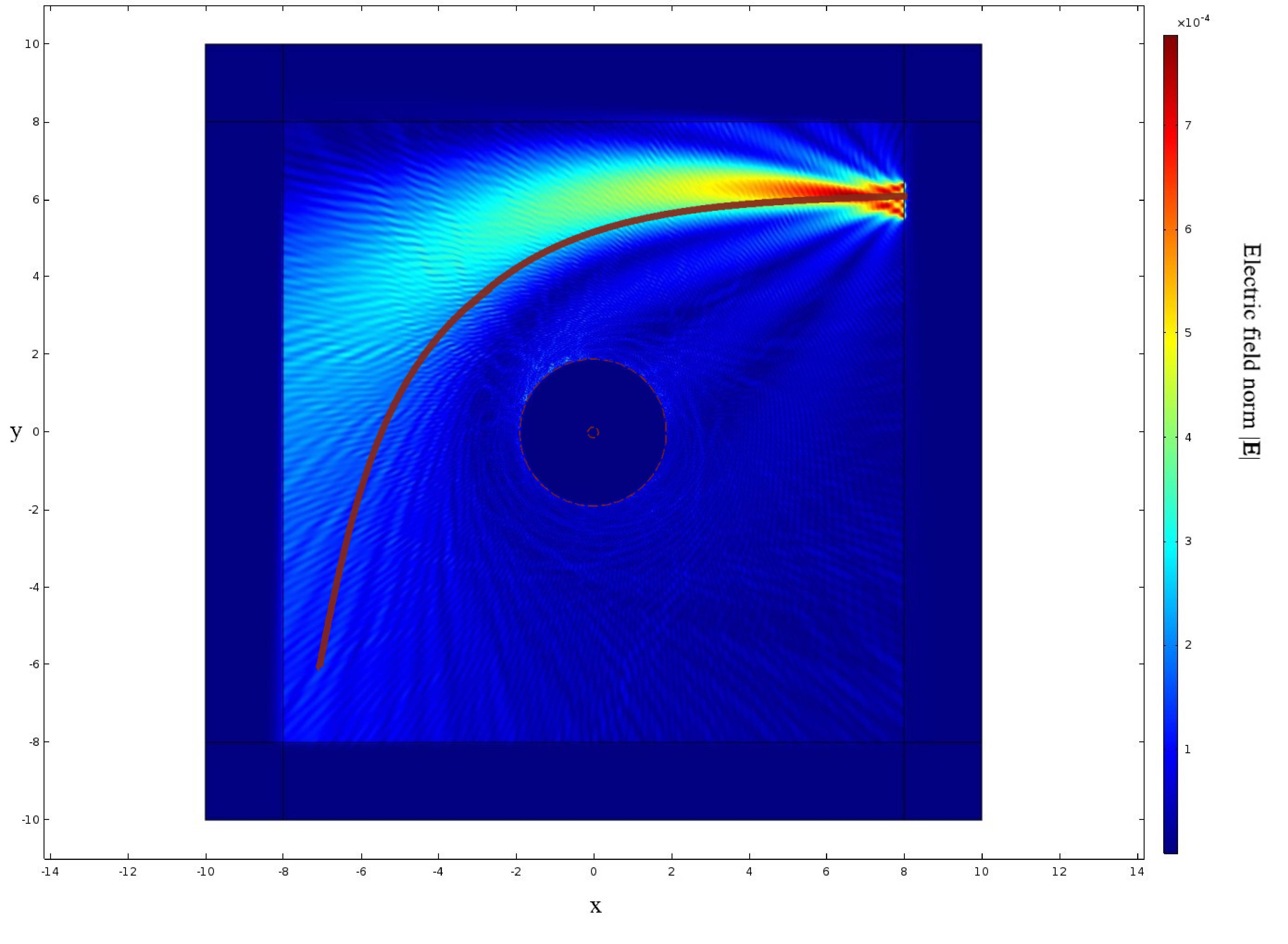
(c) $D=5.97$

Figure 3: metamaterial mimicking the Reissner-Nordström spacetime for $Q=0.5$, $m=1$ and different impact parameters, $D$.

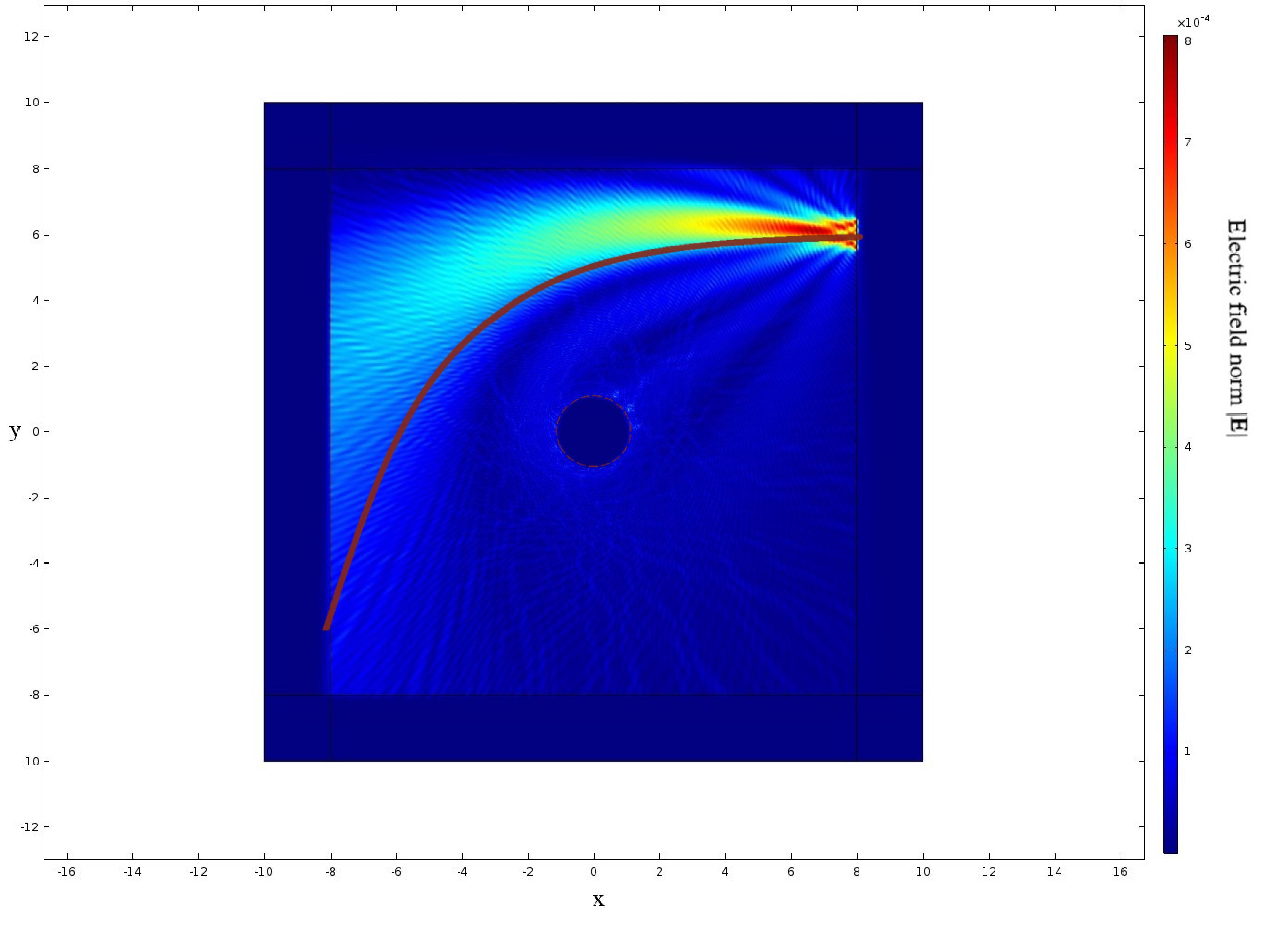
(c) $D=6$

Figure 4: metamaterial mimicking the Reissner-Nordström spacetime for $Q=1$, $m=1$ and different impact parameters, $D$.

Since photons are massless, the ray trajectories can be determined by only one character which is called the impact parameter $D=\frac{L}{E}$ mtobh . The ray trajectories can be obtained by solving Eq. (36) hakmann ; mtobh . The results for Reissner-Nordström spacetime, both for wave optics and ray optics are shown in Figs. 1-4.

Interestingly, depending on the roots of $f(r)$, we have three types of trajectories: ”terminating orbit”, ”bound orbit” and ”flyby orbit”. Those roots depend only on the impact parameter, $D$, since both $m$ and $Q$ are constants. Therefore, for $D=D_{c}$ we have ”bound orbit”, if $D>D_{c}$ there is ”flyby orbit” and if $D<D_{c}$ there is ”terminating orbit” hakmann . The critical value of impact parameter, $D_{c}$, can be driven by considering $f^{\prime}(r_{c})=0$ and $f(r_{c})=0$

$$r_{c}=\frac{3}{2}m\big{[}1+\sqrt{1-\frac{8Q^{2}}{9m^{2}}}\big{]},\hskip 14.22636ptD_{c}=\frac{r_{c}^{2}}{\sqrt{r_{c}^{2}-2mr_{c}+Q^{2}}}.$$ (37)

It is obvious that for different values of charge, $Q$, the critical value of impact parameter differs.

VI Kerr Spacetime

In this section, we are going to generalize the Schwarzschild static solution to the case of stationary one, and therefore, the Kerr spacetime is discussed. The Kerr metric describes the geometry of empty spacetime around a rotating uncharged axially-symmetric black hole with an appropriate event horizon. The Kerr metric is an exact solution of the Einstein field equations of general relativity with stationary constraint inverno . This metric in the Cartesian coordinates reads

$$ds^{2}=d\bar{t}^{2}-dx^{2}-dy^{2}-dz^{2}-\frac{2mr^{3}}{r^{4}+a^{2}z^{2}}(d\bar{t}+\frac{r(xdx+ydy)}{a^{2}+r^{2}}+\frac{a(ydx-xdy)}{a^{2}+r^{2}}+\frac{zdz}{r})^{2},$$ (38)

where $a$ and $m$ are spin parameter and geometrical mass, respectively, the radial coordinate is $r=\sqrt{x^{2}+y^{2}+z^{2}}$ and also $d\bar{t}=dt+\frac{2m(xdx+ydy+zdz)}{r^{2}-2mr+a^{2}}$.

Based on Eq. (2), permittivity and permeability tensors and $\Gamma_{i}$ in the $xy$ plane can be obtained as

$$\begin{array}[]{l}\epsilon^{xx}=\mu^{xx}=-A_{z}[\frac{-r^{8}+2mr^{7}-2r^{6}a^{2}+4m(a^{2}-\frac{y^{2}}{2})r^{5}+(-a^{4}+4mxya)r^{4}+2ma^{2}(a^{2}-x^{2})r^{3}}{(1-\frac{2m}{r})(a^{2}+r^{2})(r^{6}-2mr^{5}+r^{4}a^{2}-2m(a^{2}-r^{2})r^{3})}],\\ \\ \epsilon^{xy}=\epsilon^{yx}=\mu^{xy}=\mu^{yx}=2A_{z}[\frac{(ay+rx)(ax-ry)mr^{3}}{(1-\frac{2m}{r})(a^{2}+r^{2})(r^{6}-2mr^{5}+r^{4}a^{2}-2m(a^{2}-r^{2})r^{3})}],\\ \\ \epsilon^{xz}=\epsilon^{zx}=\mu^{xz}=\mu^{zx}=0,\\ \\ \epsilon^{yy}=\mu^{yy}=-A_{z}[\frac{-r^{8}+2mr^{7}-2r^{6}a^{2}+4m(a^{2}-\frac{x^{2}}{2})r^{5}+(-a^{4}-4mxya)r^{4}+2ma^{2}(a^{2}-y^{2})r^{3}}{(1-\frac{2mr}{r})(a^{2}+r^{2})(r^{6}-2mr^{5}+r^{4}a^{2}-2m(a^{2}-r^{2})r^{3})}],\\ \\ \epsilon^{zy}=\epsilon^{yz}=\mu^{zy}=\mu^{yz}=0,\\ \\ \epsilon^{zz}=\mu^{zz}=-A_{z}[\frac{-r^{6}+2mr^{5}-r^{4}a^{2}+2m(a^{2}-x^{2}-y^{2})r^{3}}{(1-\frac{2m}{r})(a^{2}+r^{2})(r^{6}-2mr^{5}+r^{4}a^{2}-2m(a^{2}-r^{2})r^{3})}],\end{array}$$ (39)

where $A_{z}=\sqrt{\frac{r^{4}a^{2}-2mr^{3}a^{2}+r^{6}}{r^{4}(a^{2}+r^{2})}}$. In addition, we find that

$$\begin{array}[]{l}\Gamma_{x}=-\frac{2ma(-2mr^{3}xa-r^{5}y+2r^{4}ym-r^{3}a^{2}y)}{r^{4}(r^{2}-2mr+a^{2})(a^{2}+r^{2})(1-\frac{2mr}{r})},\\ \\ \Gamma_{y}=-\frac{2ma(-2mr^{3}ya+r^{5}x-2r^{4}xm+r^{3}a^{2}x)}{r^{4}(r^{2}-2mr+a^{2})(a^{2}+r^{2})(1-\frac{2m}{r})},\\ \\ \Gamma_{z}=0.\end{array}$$ (40)

It is interesting that the vector $\vec{\Gamma}$ is non-zero because the Kerr metric is not static. It can be said that the spin parameter, $a$, makes the equivalent material bi-anisotropic. In addition, Eq. (21) can be solved numerically by considering Eqs. (39) and (40).

Regarding the Lagrangian formalism, first, we write the Kerr metric in the spherical coordinates inverno

$$ds^{2}=\frac{\Delta}{\rho^{2}}(dt-asin^{2}\theta d\phi)^{2}-\frac{sin^{2}\theta}{\rho^{2}}[(r^{2}+a^{2})d\phi-adt]^{2}-\frac{\rho^{2}}{\Delta}dr^{2}-\rho^{2}d\theta^{2},$$ (41)

where $\rho^{2}=r^{2}+a^{2}cos^{2}\theta$ and $\Delta=r^{2}-2mr+a^{2}$. Since we are working in the $xy$ plane, we set $\theta=\frac{\pi}{2}$. Substituting this metric into Eq. (22), one can show that

$$\mathcal{L}=(1-\frac{2ma^{2}}{r})\dot{t}^{2}+(\frac{4ma}{r})\dot{t}\dot{\phi}-\frac{r^{2}}{r^{2}-2mr+a^{2}}\dot{r}^{2}-[r^{2}+a^{2}+\frac{2ma^{2}}{r}]\dot{\phi}^{2}.$$ (42)

Using Eqs. (24) and (25), the following relations are obtained

$$\dot{p_{t}}=\frac{dp_{t}}{d\tau}=0,$$ (43)

$$\dot{p_{\phi}}=\frac{dp_{\phi}}{d\tau}=0$$ (44)

$$p_{t}=2(1-\frac{2m}{r})\dot{t}+\frac{4ma^{2}}{r}\dot{\phi},$$ (45)

$$p_{\phi}=\frac{4ma}{r}\dot{t}-2(r^{2}+a^{2}+\frac{2ma^{2}}{r})\dot{\phi}.$$ (46)

where, we call $p_{t}=2E$ and $p_{\phi}=-2L$, as before. By solving Eqs. (45) and (46) simultaneously, $\dot{t}$ and $\dot{\phi}$ can be calculated as

$$\dot{t}=\frac{1}{r^{2}-2mr+a^{2}}[(1-\frac{2m}{r})L+\frac{2ma}{r}E],$$ (47)

$$\dot{\phi}=\frac{1}{r^{2}-2mr+a^{2}}[(r^{2}+a^{2}+\frac{2ma^{2}}{r})E-\frac{2ma}{r}L].$$ (48)

Moreover, substituting these parameters into the Lagrangian Eq. (42), one finds

$$\mathcal{L}=(a^{2}+r^{2}+\frac{2ma^{2}}{r})E^{2}+(\frac{2m}{r})L^{2}-\frac{4ma}{r}LE-r^{2}\dot{r}^{2}.$$ (49)

Since for light beam we have $\mathcal{L}=0$,

$$\dot{r}^{2}=E^{2}+\frac{2m}{r^{3}}(aE-L)^{2}+\frac{1}{r^{2}}(a^{2}E^{2}-L^{2})=f(r).$$ (50)

It is noteworthy to mention that only the impact parameter affects the ray trajectories which its effects lead to three types of orbits mentioned in the previous section. At this point, since the equations related to Kerr spacetime are too complicated, we just focus on critical value of impact parameter. In this regard, by calculating $f^{\prime}(r_{c})=0$ and $f(r_{c})=0$, one finds mtobh

$$r_{c}=3m\frac{L-aE}{L+aE}=3m\frac{D_{c}-a}{D_{c}+a},\hskip 14.22636pt(D_{c}+a)^{3}=27m^{2}(D_{c}-a).$$ (51)

It is clear that the spin parameter, $a$, controls the critical value of the impact parameter. By considering $u=\frac{1}{r}$ and considering relations in Eqs. (50) and (51), we can rewrite Eq. (50) as

$$\dot{u}^{2}=E^{2}u^{4}m(D_{c}-a)^{2}(u-u_{c})^{2}(2u+u_{c}).$$ (52)

Taking into account $\dot{\phi}$ in Eq. (48), we can obtain

$$\frac{du}{d\phi}=\frac{(1-2mu+a^{2}u^{2})(u-u_{c})(D_{c}+a)\sqrt{2u+u_{c}}}{\sqrt{m}[3u_{c}D_{c}-2u(D_{c}+a)]}.$$ (53)

Furthermore, solving Eq. (53) gives the ray trajectories mtobh . The results for Kerr spacetime are shown in Fig. 5.

VII Results and discussion

Here, we are in a position to solve the equations of two approaches and simulate the results for comparison. Equation (21) is solved in the Cartesian coordinates and a rectangular $2D$ geometry of $xy$ space for a $TE$ polarized wave of frequency $\omega=6.3\times 10^{9}(rad/s)$ injected from the right and the results are compared with the ray path (red line) calculated from the equations of motion. The computational domain is surrounded by a perfectly matched layer that absorbs the outward waves to ensure that there are no unwanted reflections, and the simulations are done by means of a standard software solver (COMSOL).

For Reissner-Nordström spacetime the medium parameters are given by Eq. (27) and the results are depicted in Table 1 and Figs. 1-4. In order to obtain dimensionless parameters, we normalize all parameters to $r_{0}=\frac{r_{s}}{2}$ in which $r_{s}=2m$ is the event horizon of Schwarzschild black hole where the gravity is so strong, that light cannot escape mtobh .

$Q$	$D_{c}$	$r_{c}$
$0$	$5.196$	$3$
$0.1$	$5.187$	$2.99$
$0.5$	$4.97$	$2.82$
$1$	$4$	$2$

Table 1: Reissner-Nordström solutions: the numerical results of $D_{c}$ and $r_{c}$ for different values of $Q$ in the case of $m=1$.

Taking into account the plotted figures, we find that the ray path follows the center of the beam. Moreover, the ray trajectories are consistent with the behavior expected from theory. Speaking more precisely, the case of $D=D_{c}$ represents photon sphere photonsphere which is a spherical region of space where the gravitational effect is strong enough that photons are forced to travel in an orbit (in the $xy$ plane). This area is patently obvious in Figs. 1b, 2b, 3b and 4b. The photon sphere is located farther from the center of a black hole than the event horizon, the radius of photon sphere can be determined as $r_{c}$ in Eq. (37) and some numerical results of $r_{c}$ can be found in Table 1. In addition, for $D<D_{c}$, we expect that the photons are drown into the event horizon, it can be seen in Figs. 1a, 2a, 3a and 4a. Moreover, in the case of $D>D_{c}$, deflection of ray trajectory can be observed in Figs. 1c, 2c, 3c and 4c. Furthermore, it is notable that the charge of black hole, $Q$, affects the critical value of impact parameter, $D_{c}$, and as a result the radius of photon sphere, $r_{c}$ is changed. It can be seen from Table 1 that when $Q$ increases, the critical impact parameter, $D_{c}$, and radius of photon sphere, $r_{c}$, decrease.

It can be observed from all figures that the beam splits into a set of rays or sub-beams, one part falls into black hole due to having $D<D_{c}$, the other part escapes from black hole because of $D>D_{c}$ and another part bends around the photon sphere of the black hole and interferes with the primary beam.

It is expected from theory that the case of $Q=0$ represents Schwarzschild spacetime. The radius of photon sphere is determined $r_{c}=3m$ for $Q=0$ that is similar to our expectation, also Fig. 1 matches the results reported in Ref. schwarz3 .

For the Kerr spacetime the medium parameters are given by Eqs. (39) and (40), while the numerical and simulated results are shown in Table 2 and Fig. 5. It is notable that in order to have dimensionless parameters, they are normalized to $r_{s}$, as before.

$a$	$D_{c}$	$r_{c}$
$+0.1$	$2.48$	$1.38$
$0$	$2.60$	$1.5$
$-0.1$	$2.74$	$1.61$
$-0.5$	$3.5$	$2$

Table 2: Kerr solutions: the numerical results of $D_{c}$ and $r_{c}$ for different values of $a$ in the case of $m=1$.

As we mentioned before, computational analysis of rotating spacetime is complicated, and therefore, we just focus on the critical values of the impact parameter which lead to photon sphere. In contrast to the Reissner-Nordström black hole, the Kerr black hole is not spherical symmetry, but only enjoys axially symmetry, which has profound consequences for the photon orbits. A circular orbit can only exist in the equatorial plane photonsphere . Fortunately, both methods of simulations, numeric solutions to Maxwell equations and the ray trajectory arisen from the Hamiltonian formalism, are in agreement to each others. As it is depicted in Table 2, by decreasing the spin parameter ($a$), the critical impact parameter ($D_{c}$) and the radius of photon sphere ($r_{c}$) increase. In addition, in the case of static case ($a=0$), the results of the Kerr black hole match to that of driven from Schwarzschild black hole, as expected.

VIII Concluding Remarks

Here, we compared geometrical description of gravitational systems with optical media in flat space with two approaches. We observed a good correspondence between the two methods.

We considered two supplementary factors of the Schwarzschild black hole; the electric charge and rotation parameters. More precisely, we investigated the effects of electric charge and rotation factors on the trajectory of light with various impact parameters. We found that the medium parameters given for Reissner-Nordström and Kerr spacetime can mimic the ray path near the black hole in the flat spacetime. Interestingly, some theoretical phenomena like photon sphere are observed and the effects of charge, $Q$, and spin parameter, $a$, are investigated. We showed that the critical impact parameter is a decreasing function of both the electric charge and spin parameters. This behavior is expected due to the fact that increasing the electric charge and rotation lead to decreasing the event horizon radius (weaken the gravitational effect) in the classical black hole scenario.

It will be interesting to apply these calculations to the Kerr Newman black hole and other interesting nontrivial solutions of Einstein gravity.

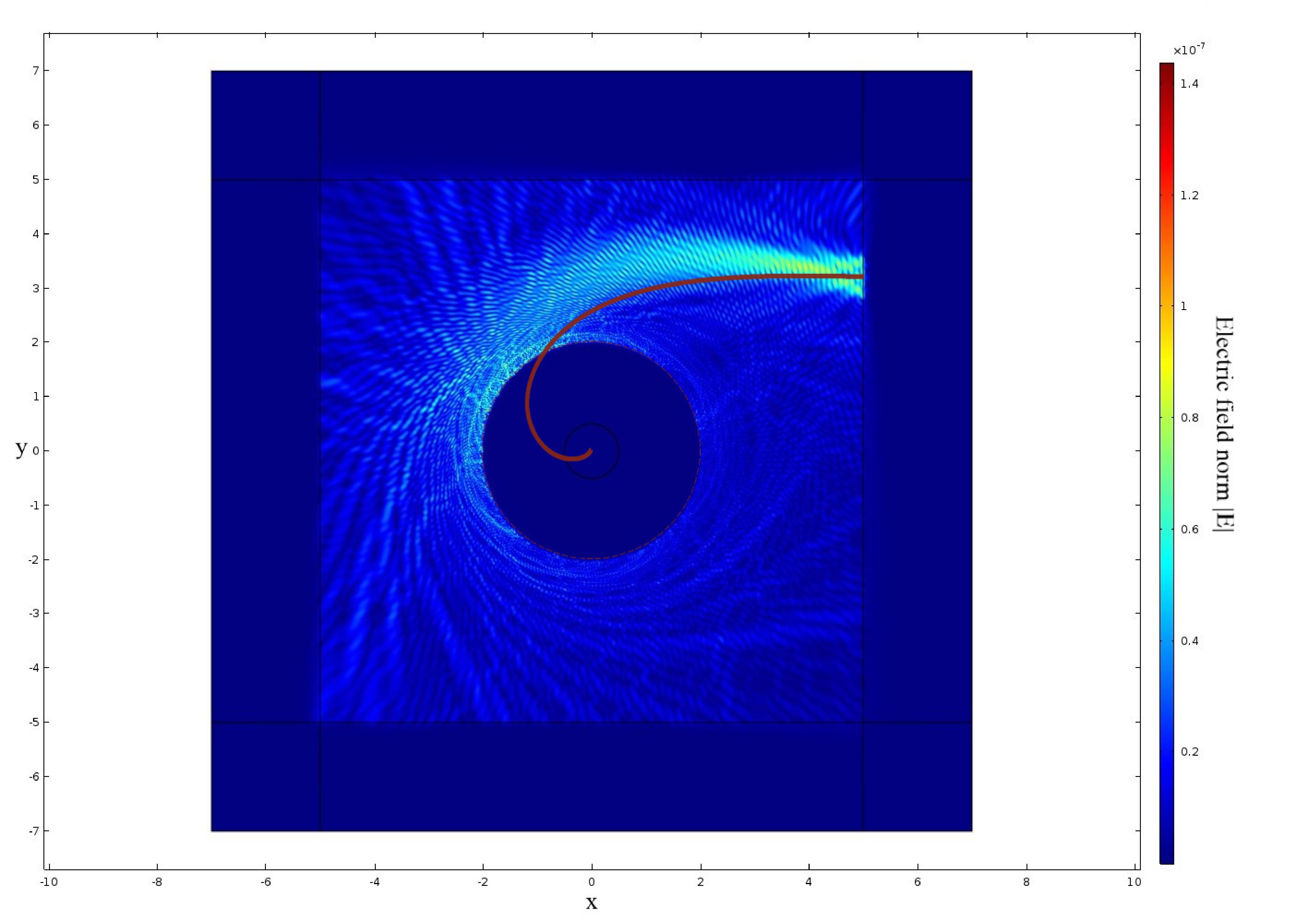
(a) $D=3.2$

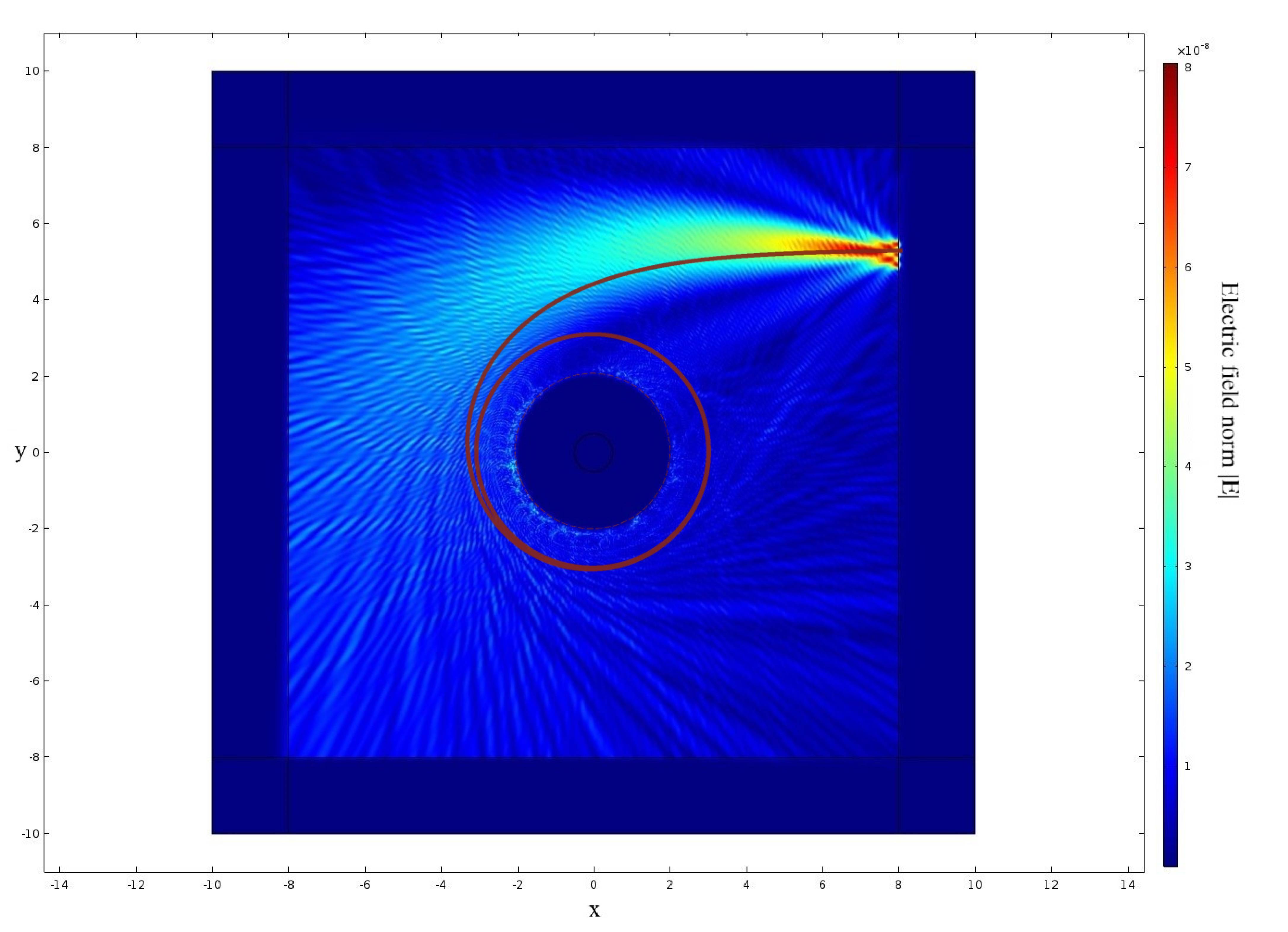
(b) $D=5.2$

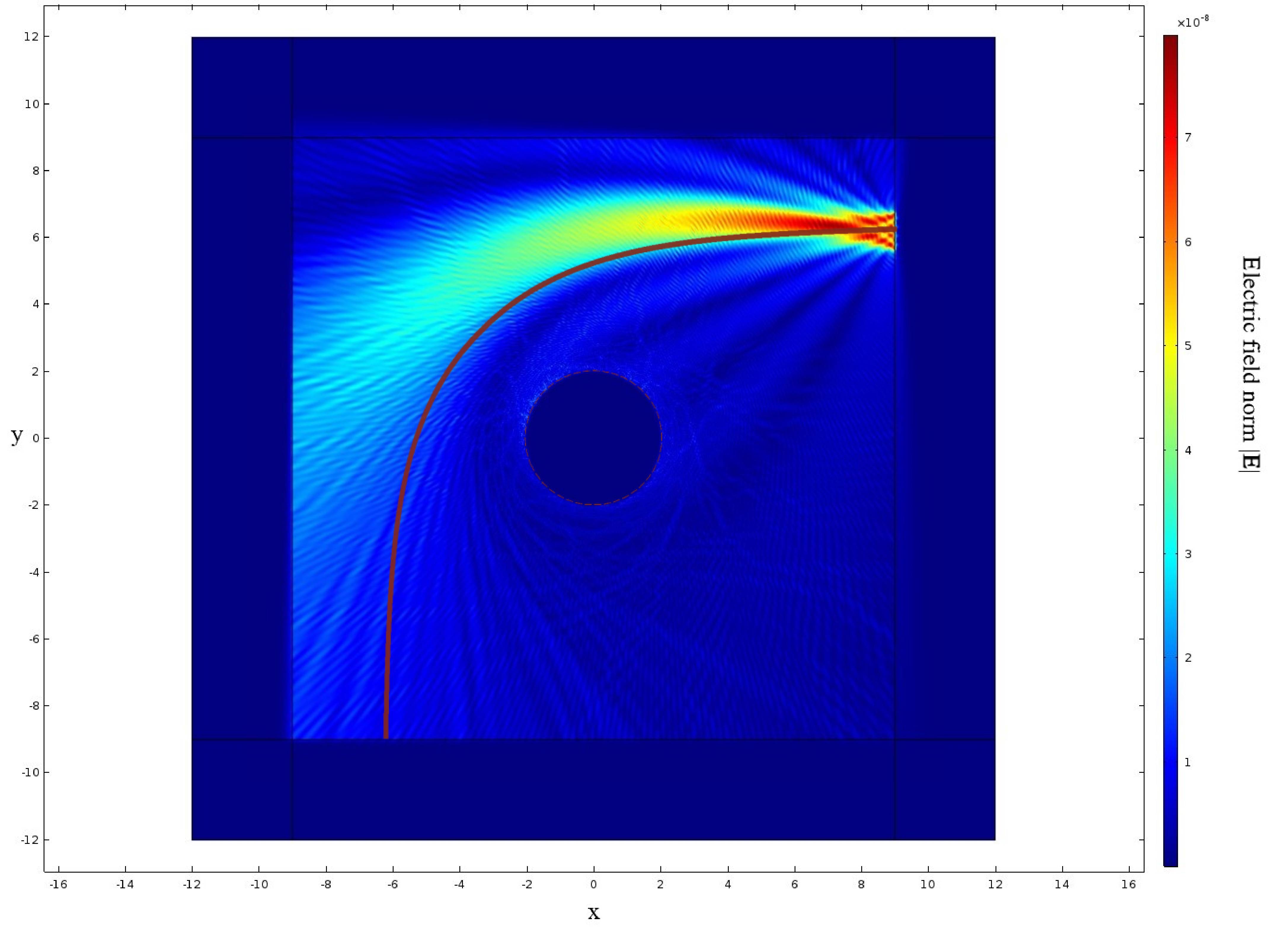
(c)

Figure 1: metamaterial mimicking the Reissner-Nordström spacetime for $Q=0$, $m=1$ and different impact parameters, $D$.

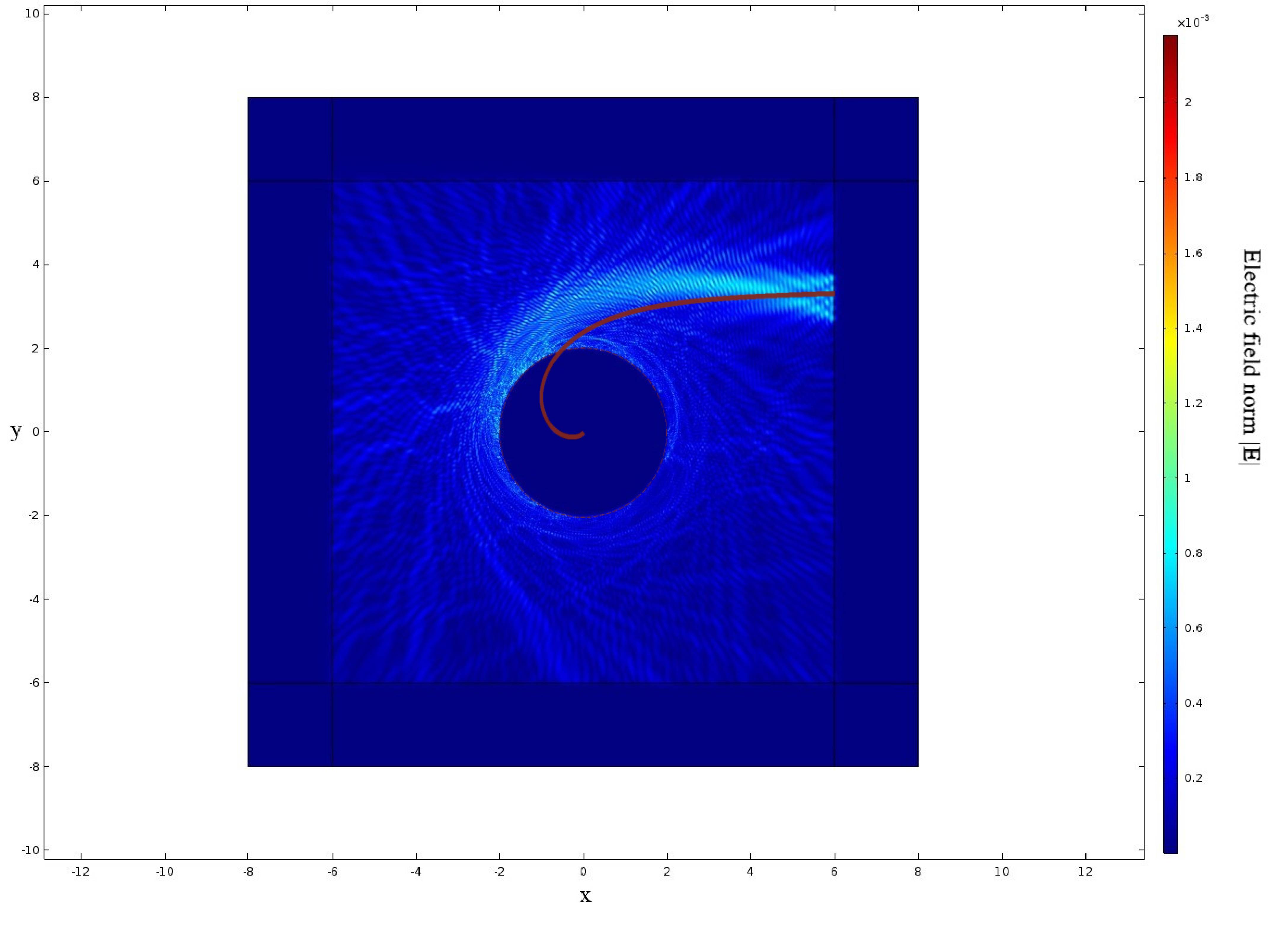
(a) $D=3.2$

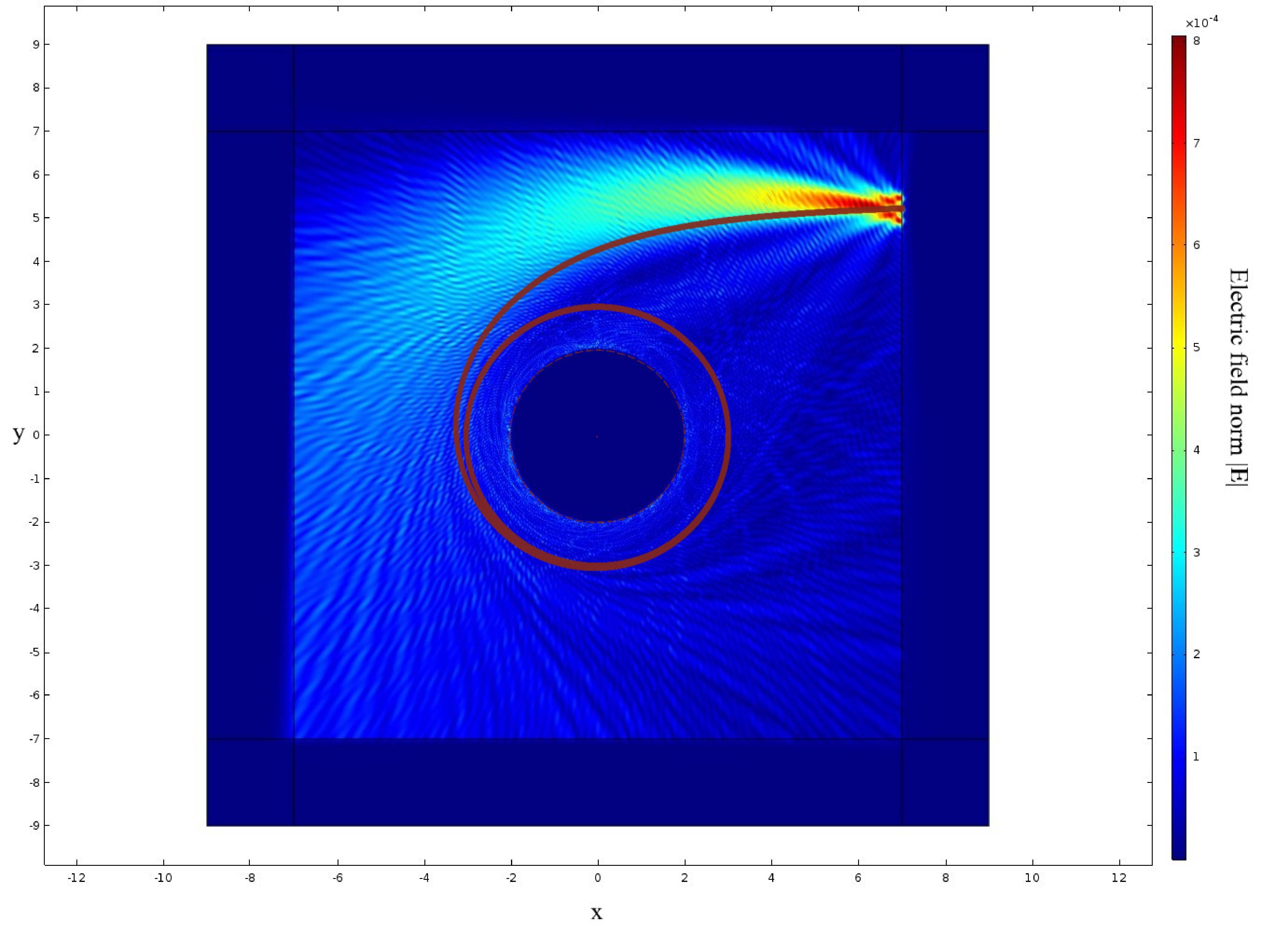
(b) $D=5.2$

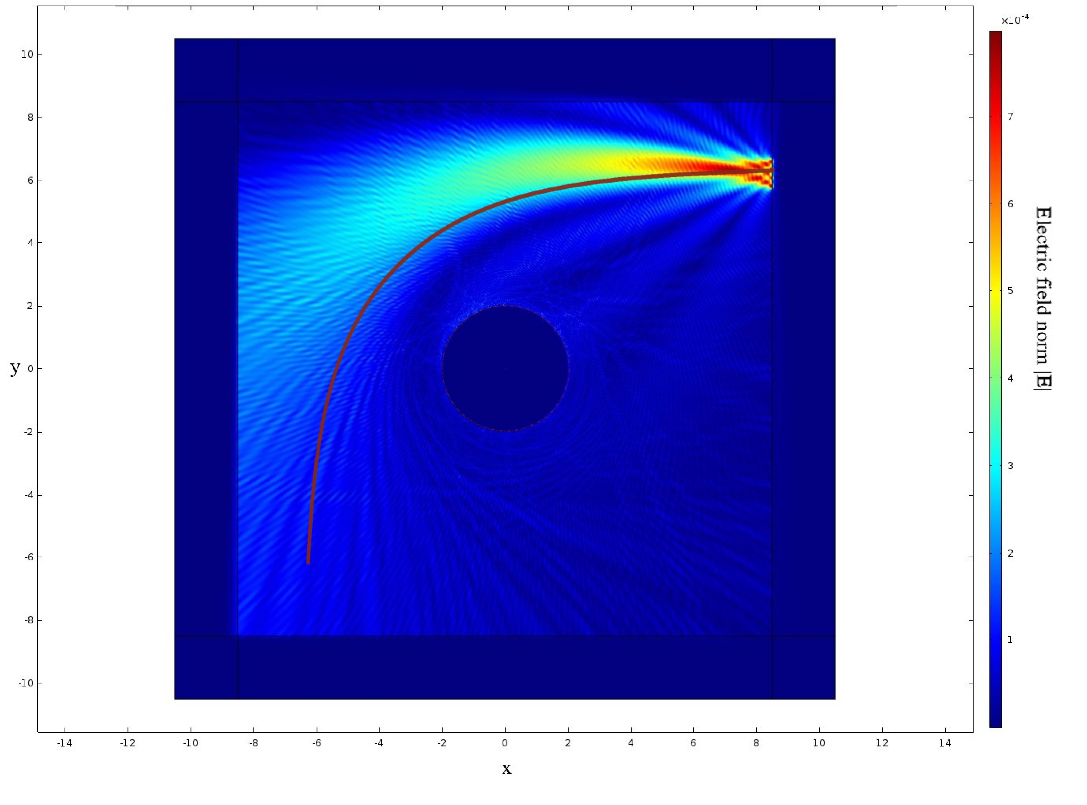
(c) $D=6.2$

Figure 2: metamaterial mimicking the Reissner-Nordström spacetime for $Q=0.1$, $m=1$ and different impact parameters, $D$.

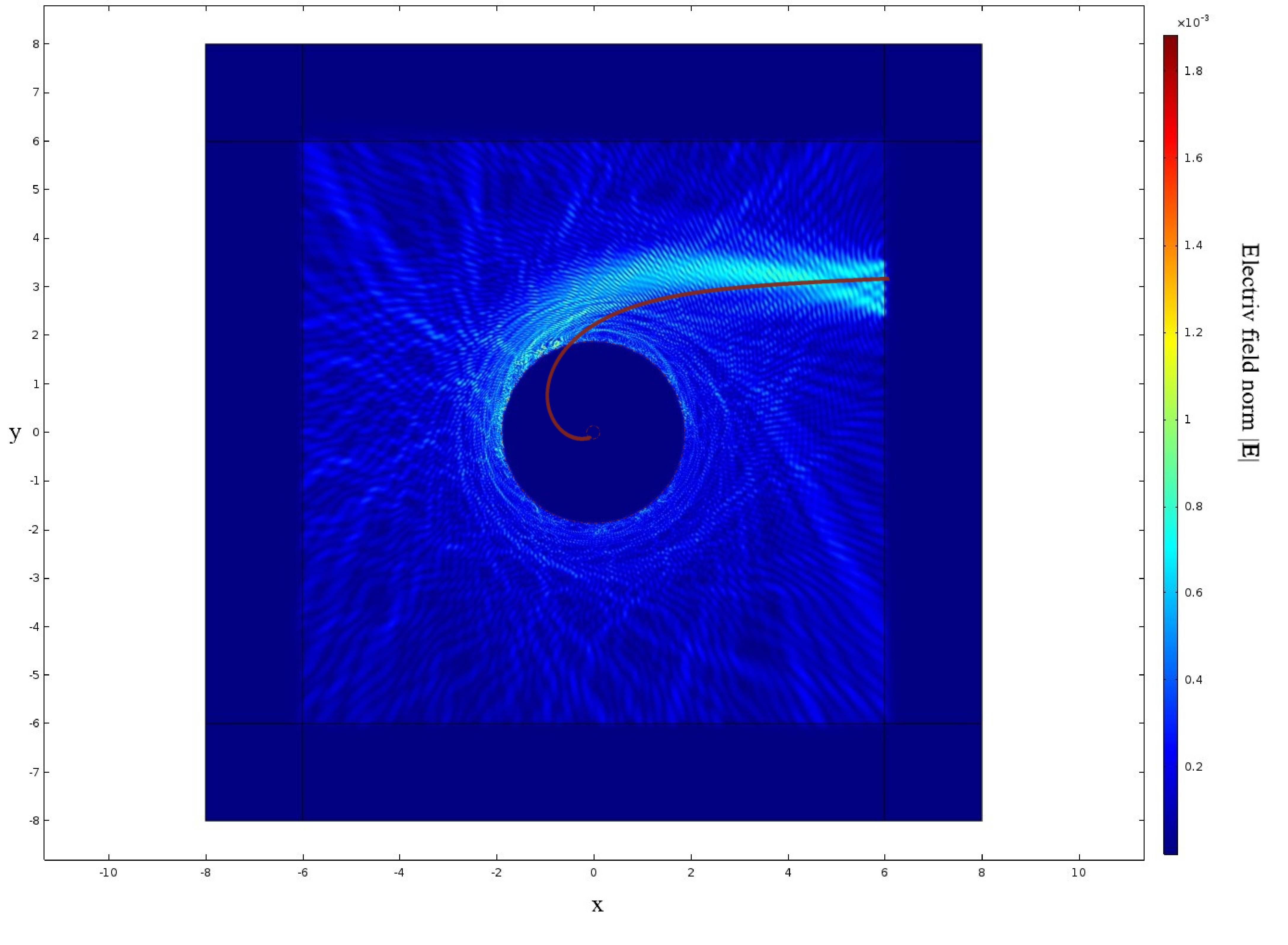
(a) $D=2.97$

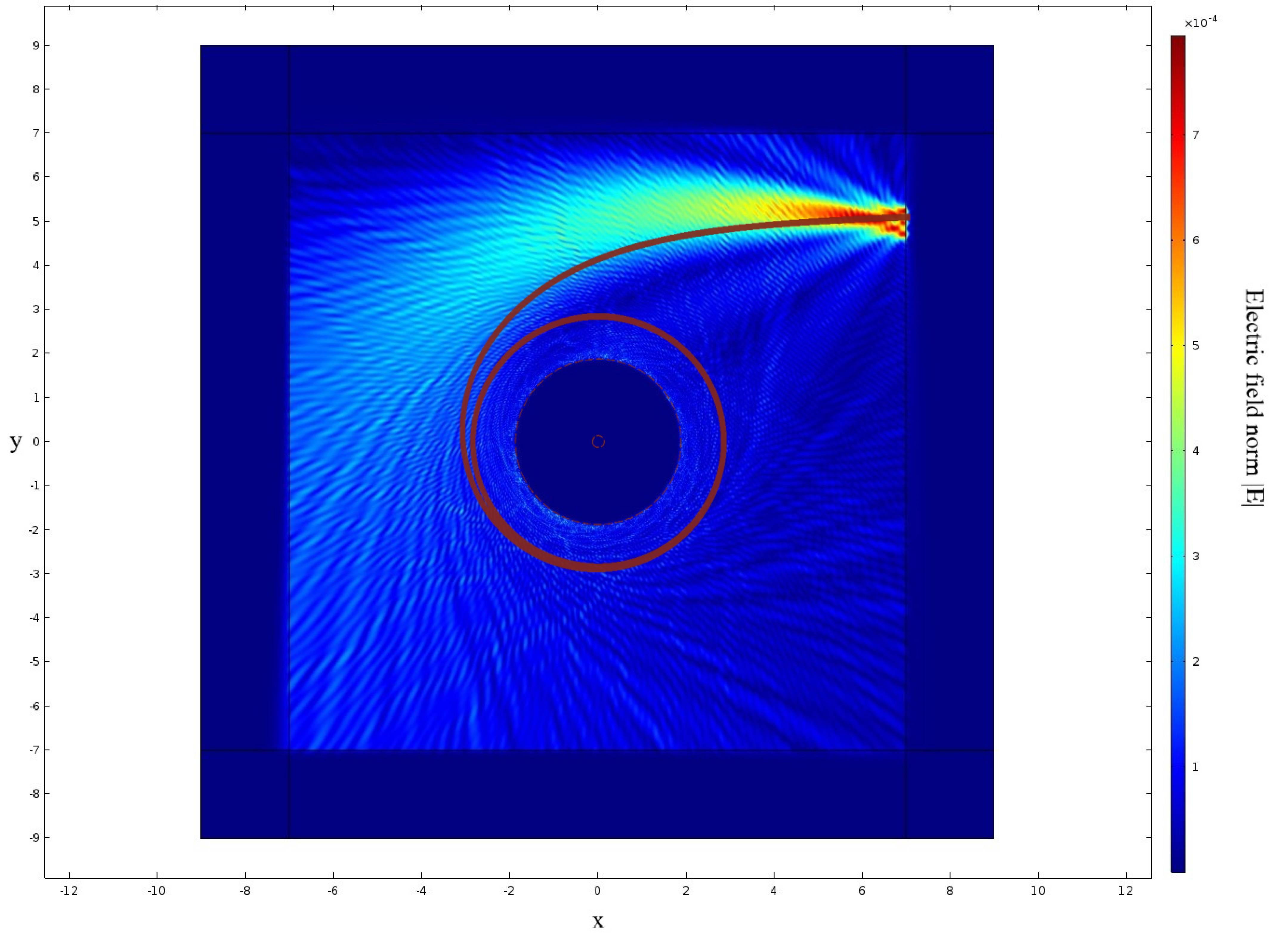
(b) $D=4.97$

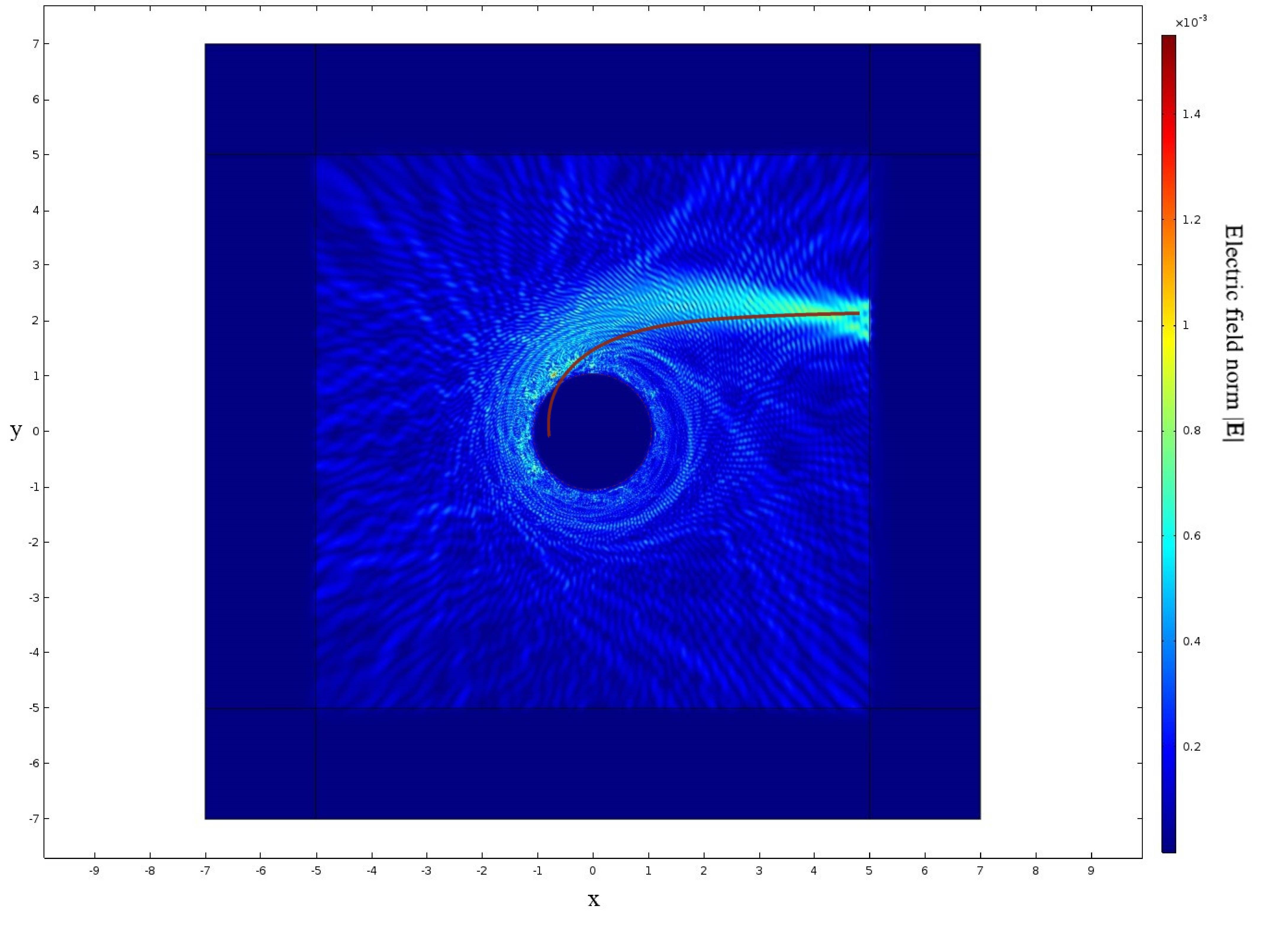
(a) $D=2$

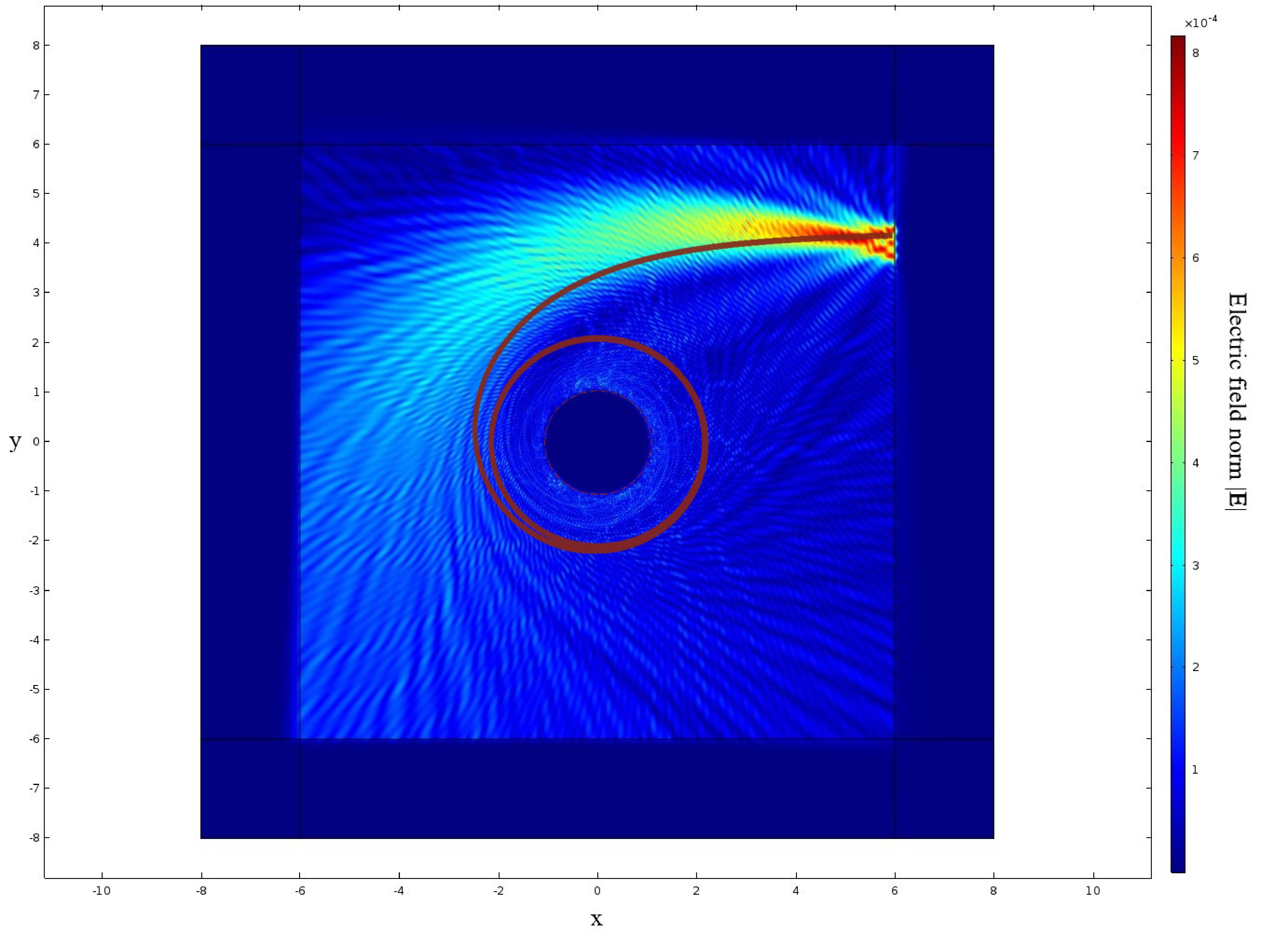
(b) $D=4$

(a) $a=+0.1,D=2.48$

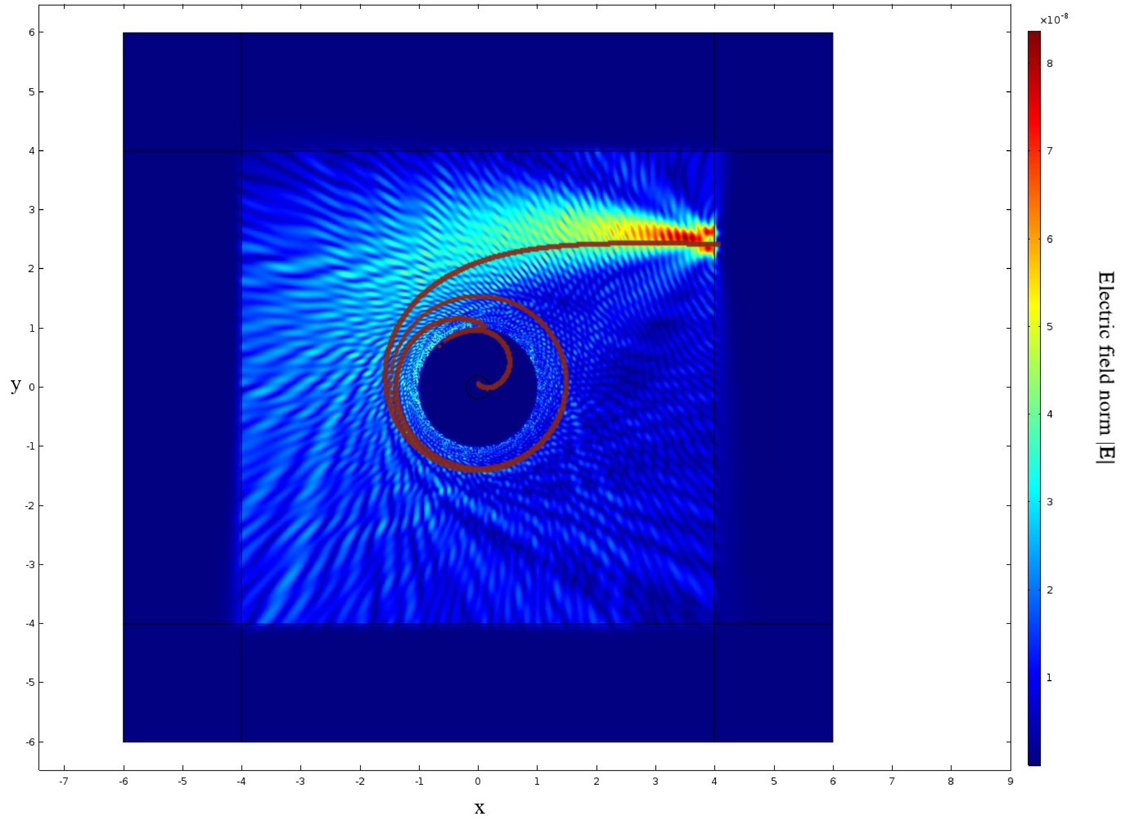
(b) $a=-0.1,D=2.74$

(c) $a=-0.5,D=3.5$

Figure 5: metamaterial mimicking the Kerr spacetime for $m=0.5$ and different impact parameters, $D$, and spin parameters, $a$.

IX Acknowledgements

We wish to thank Shiraz University Research Council. This work has been supported financially by the Research Institute for Astronomy and Astrophysics of Maragha, Iran.

References

- (1) W. Gordon, Ann. Phys. (Leipzig) 72, 421 (1923).
- (2) C. Barcelo, S. Liberati, and M. Visser, Living Rev. Relativ. 8, 12 (2005).
- (3) M. Visser, Class. Quantum Gravit. 15, 1767 (1998).
- (4) U. Leonhardt and T. G. Philbin, New J. Phys. 8, 247 (2006).
- (5) U. Leonhardt and T. G. Philbin, Prog. Opt. 53, 70 (2009).
- (6) U. Leonhardt and T. G. Philbin, Geometry and Light: The Science of Invisibility, (New York: Dover Publ, 2010)
- (7) D. A. Genov, S. Zhang and X. Zhang, Nature Phys. 5, 687 (2009).
- (8) U. Leonhardt and T. G. Philbin, New J. Phys. 8, 247 (2006).
- (9) Igor I. Smolyaninov, J. Opt. 13, 024004 (2011).
- (10) E. E. Narimanov and A. V. Kildishev, Appl. Phys. Lett. 95, 041106 (2009).
- (11) Q. Cheng, T.J. Cui, W. X. Jiang and B. G. Cai, New J. Phys. 12, 063006 (2010).
- (12) Y. R. Yang, L. Y. Leng, N. Wang, Y. G. Ma and C. K. Ong, J. Opt. Soc. Am. A 29, 473 (2012).
- (13) M. Yin, X. Tian, L. Wu and D. Li, Opt. Exp. 21, 19082 (2013).
- (14) C. Sheng, H. Liu, Y. Wang, S. N. Zhu and D. A. Genov, Nature Photon. 7, 902 (2013).
- (15) R. T. Thompson and J. Frauendiener, Phys. Rev. D 82, 124021 (2010).
- (16) H. Chen, R-X. Miao and M. Li, Opt. Exp. 18, 15183 (2010).
- (17) I. Fernandez-Nunez and O. Bulashenko, Phys. Lett. A 380, 1 (2016).
- (18) R. Schutzhold, G. Plunien and G. Soff, Phys. Rev. Lett. 88, 061101 (2002).
- (19) J. Plebanski, Phys. Rev. 118, 1396 (1960).
- (20) R. Marques, F. Medina and R. Rafii-El-Idrissi, Phys. Rev. B 65, 144440 (2002).
- (21) M. S. Rill, C. E. Kriegler, M. Thiel, G. Freymann, S. Linden and M. Wegener, Opt. Lett. 34, 1921 (2009).
- (22) T. G. Mackay and A. Lakhtakia, Electromagnetic Anisotropy and Bianisotropy: A Field Guide, (World Scientific, 2010).
- (23) A. Serdyukov, I. Semchenko, S. Tretyakov and A. Sihvola, Electromagnetics of Bi-anisotropic Materials, (Gordon and Breach, Amsterdam, 2001).
- (24) A. H. Sihvola, A. J. Viitanen, I. V. Lindell and S. A. Tretyakov, Electro magnetic Waves in Chiral and Bi-Isotropic Media, (Artech House, Norwood, 1994).
- (25) D. Pile, Nature Photonics 6, 5 (2012).
- (26) U. Leonhardt and T. G. Philbin, Prog. Opt. 53, 69 (2009).
- (27) J. D. Jackson, Classical Electrodynamics , (Wiley, New York, 1999).
- (28) Y. Liu, B. Gralak, S. Guenneau, Opt. Exp. 24, 26479 (2016).
- (29) R. d‘Inverno, Introducing Einstein’s Relativity, (Oxford University Press, 1992).
- (30) S. Chandrasekhar, The mathematical theory of black holes, (Clarendon Press-Oxford University Press, 1983).
- (31) E. Hackmann, B. Hartmann, C. Lammerzahl and P. Sirimachan, Phys. Rev. D 81, 064016 (2010).
- (32) D. Nitta, T. Chiba and N. Sugiyama, Phys. Rev. D. 84, 063008 (2011).