AD3: Attentive Deep Document Dater

Abstract

Knowledge of the creation date of documents facilitates several tasks such as summarization, event extraction, temporally focused information extraction etc. Unfortunately, for most of the documents on the Web, the time-stamp metadata is either missing or can’t be trusted. Thus, predicting creation time from document content itself is an important task. In this paper, we propose Attentive Deep Document Dater (AD3), an attention-based neural document dating system which utilizes both context and temporal information in documents in a flexible and principled manner. We perform extensive experimentation on multiple real-world datasets to demonstrate the effectiveness of AD3 over neural and non-neural baselines.

1 Introduction

Many natural language processing tasks require document creation time (DCT) information as a useful additional metadata. Tasks such as information retrieval Li and Croft (2003); Dakka et al. (2008), temporal scoping of events and facts Allan et al. (1998); Talukdar et al. (2012b), document summarization Wan (2007) and analysis de Jong et al. (2005a) require precise and validated creation time of the documents. Most of the documents obtained from the Web either contain DCT that cannot be trusted or contain no DCT information at all Kanhabua and Nørvåg (2008). Thus, predicting the time of these documents based on their content is an important task, often referred to as Document Dating.

A few generative approaches de Jong et al. (2005b); Kanhabua and Nørvåg (2008) as well as a discriminative model Chambers (2012) have been previously proposed for this task. Kotsakos et al. (2014) employs term-burstiness resulting in improved precision on this task.

Recently proposed NeuralDater Vashishth et al. (2018) uses a graph convolution network (GCN) based approach for document dating, outperforming all previous models by a significant margin. NeuralDater extensively uses the syntactic and temporal graph structure present within the document itself. Motivated by NeuralDater, we explicitly develop two different methods: a) Attentive Context Model, and b) Ordered Event Model. The first component tries to accumulate knowledge across documents, whereas the latter uses the temporal structure of the document for predicting its DCT.

Motivated by the effectiveness of attention based models in different NLP tasks Yang et al. (2016a); Bahdanau et al. (2014), we incorporate attention in our method in a principled fashion. We use attention not only to capture context but also for feature aggregation in the graph convolution network Hamilton et al. (2017). Our contributions are as follows.

• We propose Attentive Deep Document Dater (AD3), the first attention-based neural model for time-stamping documents.

• We devise a novel method for label based attentive graph convolution over directed graphs and use it for the document dating task.

• Through extensive experiments on multiple real-world datasets, we demonstrate AD3’s effectiveness over previously proposed methods.

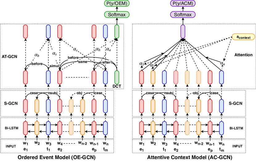
Figure 1: Two proposed models a) Ordered Event Model (left) and b) Attentive Context Model (right), where $\text{w}_{\text{i}}$ are the words of a document (D), $\text{e}_{\text{i}}$ are the words signifying events and $\text{t}_{\text{i}}$ are the temporal tokens as detected in the document. Both models use Bi-LSTM and S-GCN (Syntactic-GCN, see Section 3.2.2) in the initial part of their pipeline. Ordered Event Model (OE-GCN) uses a label based attentive graph convolutional network for encoding the DCT, whereas Attentive Context Model (AC-GCN) uses a word attention based model to encode the document. $\alpha_{i}(\forall\ i\in[1,n])$ denotes attention over the words of document and $\alpha_{a},\ \alpha_{b}$ and $\alpha_{s}$ denote attention over nodes connected with edge labels AFTER, BEFORE and SIMULTANEOUS, respectively. OE-GCN provides the probability scores over the years given the encoded DCT, while AC-GCN provides the probability scores given the context of the document. Both the models are trained separately.

AD3 source code and datasets used in the paper are available at https://github.com/malllabiisc/AD3

2 Related Work

Document Time-Stamping: Initial attempts made for document time-stamping task include statistical language models proposed by de Jong et al. (2005b) and Kanhabua and Nørvåg (2008). Chambers (2012) use temporal and hand-crafted features extracted from documents to predict DCT. They propose two models, one of which learns the probabilistic constraints between year mentions and the actual creation time, whereas the other one is a discriminative model trained on hand-crafted features. Kotsakos et al. (2014) propose a term-burstiness Lappas et al. (2009) based statistical method for the task. Vashishth et al. (2018) propose a deep learning based model which exploits the temporal and syntactic structure in documents using graph convolutional networks (GCN).

Event Ordering System: The task of extracting temporally rich events and time expressions and ordering between them is introduced in the TempEval challenge UzZaman et al. (2013); Verhagen et al. (2010). Various approaches McDowell et al. (2017); Mirza and Tonelli (2016) made for solving the task use sieve-based architectures, where multiple classifiers are ranked according to their precision and their predictions are weighted accordingly resulting in a temporal graph structure. A method to extract temporal ordering among relational facts was proposed in Talukdar et al. (2012a).

Graph Convolutional Network (GCN): GCN Kipf and Welling (2016) is the extension of convolutional networks over graphs. In different NLP tasks such as semantic-role labeling Marcheggiani and Titov (2017), neural machine translation Bastings et al. (2017), and event detection Nguyen and Grishman (2018), GCNs have proved to be effective. We extensively use GCN for capturing both syntactic and temporal aspect of the document.

Attention Network: Attention networks have been well exploited for various tasks such as document classification Yang et al. (2016b), question answering Yang et al. (2016a), machine translation Bahdanau et al. (2014); Vaswani et al. (2017). Recently, attention over graph structure has been shown to work well by Veličković et al. (2018). Taking motivation from them, we deploy an attentive convolutional network on temporal graph for the document dating problem.

3 Background: GCN & NeuralDater

The task of document dating can be modeled as a multi-class classification problem. Following prior work, we shall focus on DCT prediction at the year-granularity in this paper. In this section, we summarize the previous state-of-the-art model NeuralDater Vashishth et al. (2018), before moving onto our method. An overview of graph convolutional network (GCN) Kipf and Welling (2016) is also necessary as it is used in NeuralDater as well as in our model.

3.1 Graph Convolutional Network

GCN for Undirected Graph: Consider an undirected graph, $\mathcal{G}=(\mathcal{V},\mathcal{E})$, where $\mathcal{V}$ and $\mathcal{E}$ are the set of $n$ vertices and set of edges respectively. Matrix $\mathcal{X}\in\mathbb{R}^{n\times m}$, whose rows are input representation of node $u$, where $x_{u}\in\mathbb{R}^{m}\text{, }\ \forall\ u\in\mathcal{V}$, is the input feature matrix. The output hidden representation $h_{v}\in\mathbb{R}^{d}$ of a node $v$ after a single layer of graph convolution operation can be obtained by considering only the immediate neighbours of $v$, as formulated in Kipf and Welling (2016). In order to capture information at multi-hop distance, one can stack layers of GCN, one over another.

GCN for Directed Graph: Consider a labelled edge from node $u$ to $v$ with label $l(u,v)$, denoted collectively as $(u,v,l(u,v))$. Based on the assumption that information in a directed edge need not only propagate along its direction, Marcheggiani and Titov (2017) added opposite edges viz., for each $(u,v,l(u,v))$, $(v,u,l(u,v)^{-1})$ is added to the edge list. Self loops are also added for passing the current embedding information. When GCN is applied over this modified directed graph, the embedding of the node $v$ after $k^{th}$ layer will be,

$$h_{v}^{k+1}=f\left(\sum_{u\in\mathcal{N}(v)}\left(W^{k}_{l(u,v)}h_{u}^{k}+b^{k}_{l(u,v)}\right)\right).$$

We note that the parameters $W^{k}_{l(u,v)}$ and $b^{k}_{l(u,v)}$ in this case are edge label specific. $h^{k}_{u}$ is the input to the $k^{th}$ layer. Here, $\mathcal{N}(v)$ refers to the set of neighbours of $v$, according to the updated edge list and $f$ is any non-linear activation function (e.g., ReLU: $f(x)=\max(0,x)$).

3.2 NeuralDater

In this sub-section, we provide a brief overview of the components of the NeuralDater Vashishth et al. (2018). Given a document $D$ with $n$ tokens $w_{1},w_{2},\cdots w_{n}$, NeuralDater extracts a temporally rich embedding of the document in a principled way as explained below:

3.2.1 Context Embedding

Bi-directional LSTM is employed for embedding each word with its context. The GloVe representation of the words $X\in\mathbb{R}^{n\times k}$ is transformed to a context aware representation $H^{cntx}\in\mathbb{R}^{n\times k}$ to get the context embedding. This is essentially shown as the Bi-LSTM in Figure 1.

3.2.2 Syntactic Embedding

In this step, the context embeddings are further processed using GCN over the dependency parse tree of the sentences in the document, in order to capture long range connection among words. The syntactic dependency structure is extracted by Stanford CoreNLP’s dependency parser Manning et al. (2014). NeuralDater follows the same formulation of GCN for directed graph as described in Section 3.1, where additional edges are added to the graph to model the information flow. Again following Marcheggiani and Titov (2017), NeuralDater does not allocate separate weight matrices for different types of dependency edge labels, rather it considers only three type of edges: a) edges that exist originally, b) the reverse edges that are added explicitly, and c) self loops. The S-GCN portion of Figure 1 represents this component.

More formally, $H^{cntx}\in\mathbb{R}^{n\times k}$ is transformed to $H^{syn}\in\mathbb{R}^{n\times k_{syn}}$ by applying S-GCN.

3.2.3 Temporal Embedding

In this layer, NeuralDater exploits the Event-Time graph structure present in the document. CATENA Mirza and Tonelli (2016), current state-of-the-art temporal and causal relation extraction algorithm, produces the temporal graph from the event time annotation of the document. GCN applied over this Event-Time graph, namely T-GCN, chooses $n_{T}$ number of tokens out of total $n$ tokens from the document for further revision in their embeddings. Note that T is the total number of events and time mentions present in the document. A special node DCT is added to the graph and its embedding is jointly learned. Note that this layer learns both label and direction specific parameters.

3.2.4 Classifier

Finally, the DCT embedding concatenated with the average pooled syntactic embedding is fed to a softmax layer for classification. This whole procedure is trained jointly.

4 Attentive Deep Document Dater (AD3): Proposed Method

In this section, we describe Attentive Deep Document Dater (AD3), our proposed method. AD3 is inspired by NeuralDater, and shares many of its components. Just like in NeuralDater, AD3 also leverages two main types of signals from the document – syntactic and event-time – to predict the document’s timestamp. However, there are crucial differences between the two systems. Firstly, instead of concatenating embeddings learned from these two sources as in NeuralDater, AD3 treats these two models completely separate and combines them at a later stage. Secondly, unlike NeuralDater, AD3 employs attention mechanisms in each of these two models. We call the resulting models Attentive Context Model (AC-GCN) and Ordered Event Model (OE-GCN). These two models are described in Section 4.1 and Section 4.2, respectively.

4.1 Attentive Context Model (AC-GCN)

Recent success of attention-based deep learning models for classification Yang et al. (2016b), question answering Yang et al. (2016a), and machine translation Bahdanau et al. (2014) have motivated us to use attention during document dating. We extend the syntactic embedding model of NeuralDater (Section 3.2.2) by incorporating an attentive pooling layer. We call the resulting model AC-GCN. This model (right side in Figure 1) has two major components.

• Context Embedding and Syntactic Embedding: Following NeuralDater, we used Bi-LSTM and S-GCN to capture context and long-range syntactic dependencies in the document (Please refer to Section 3.2.1, Section 3.2.2 for brief description). The syntactic embedding, $H^{syn}\in\mathbb{R}^{n\times k_{syn}}$ is then fed to an Attention Network for further processing. Note that, $k_{syn}$ is the dimension of the output of Syntactic-GCN and $n$ is the number of tokens in the document.

• Attentive Embedding: In this layer, we learn the representation for the whole document through word level attention network. We learn a context vector, $u_{s}\in\mathbb{R}^{s}$ with respect to which we calculate attention for each token. Finally, we aggregate the token features with respect to their attention weights in order to represent the document. More formally, let $h^{syn}_{t}\in\mathbb{R}^{k_{syn}}$ be the syntactic representation of the $t^{th}$ token in the document. We take non-linear projection of it in $\mathbb{R}^{s}$ with $W_{s}\in\mathbb{R}^{s\times k_{syn}}$. Attention weight $\alpha_{t}$ for $t^{th}$ token is calculated with respect to the context vector $u_{t}^{T}$ as follows.

  $$u_{t}=\mathrm{tanh}(W_{s}h^{syn}_{t}),$$

  $$\alpha_{t}=\frac{\mathrm{exp}(u_{t}^{T}u_{s})}{\sum_{t}\mathrm{exp}(u_{t}^{T}u_{s})}.$$

  Finally, the document representation for the AC-GCN is computed as shown below.

  $$d_{\mathrm{AC-GCN{}}}=\sum_{t}\alpha_{t}h^{syn}_{t}$$

  This representation is fed to a softmax layer for the final classification.

The final probability distribution over years predicted by the AC-GCN is given below.

$$\mathrm{P}_{\mathrm{AC-GCN{}}}(y|D)=\mathrm{Softmax}(W\cdot d_{\mathrm{AC-GCN{}}}+b).$$

4.2 Ordered Event Model (OE-GCN)

The OE-GCN model is shown on the left side of Figure 1. Just like in AC-GCN, context and syntactic embedding is also part of OE-GCN. The syntactic embedding is fed to the Attentive Graph Convolution Network (AT-GCN) where the graph is obtained from the time-event ordering algorithm CATENA Mirza and Tonelli (2016). We describe these components in detail below.

4.2.1 Temporal Graph

We use the same process used in NeuralDater Vashishth et al. (2018) for procuring the Temporal Graph from the document. CATENA Mirza and Tonelli (2016) generates 9 different temporal links between events and time expressions present in the document. Following Vashishth et al. (2018), we choose 5 most frequent ones - AFTER, BEFORE, SIMULTANEOUS, INCLUDES, and IS INCLUDED – as labels. The temporal graph is constructed from the partial ordering between event verbs and time expressions.

Let $\mathcal{E}_{T}$ be the edge list of the Temporal Graph. Similar to Marcheggiani and Titov (2017); Vashishth et al. (2018), we also add reverse edges for each of the existing edge and self loops for passing current node information as explained in Section 3.1. The new edge list $\mathcal{E}_{T}^{{}^{\prime}}$ is shown below.

$$\mathcal{E^{\prime}_{\text{T}}}=\mathcal{E_{\text{T}}}\cup\{(j,i,l(i,j)^{-1})~{}|~{}(i,j,l(i,j))\in\mathcal{E_{\text{T}}}\}\\ \cup\{(i,i,\mathrm{self})~{}|~{}i\in\mathcal{V})\}.$$

The reverse edges are added with reverse labels like $\mathrm{AFTER}^{-1}$, $\mathrm{BEFORE}^{-1}$ etc . Finally, we get 10 labels for our temporal graph and we denote the set of edge labels by $\mathcal{L}$.

4.2.2 Attentive Graph Convolution (AT-GCN)

Since the temporal graph is automatically generated, it is likely to have incorrect edges. Ideally, we would like to minimize the influence of such noisy edges while computing temporal embedding. In order to suppress the noisy edges in the Temporal Graph and detect important edges for reasoning, we use attentive graph convolution Hamilton et al. (2017) over the Event-Time graph. The attention mechanism learns the aggregation function jointly during training. Here, the main objective is to calculate the attention over the neighbouring nodes with respect to the current node for a given label. Then the embedding of the current node is updated by mixing neighbouring node embedding according to their attention scores. In this respect, we propose a label-specific attentive graph convolution over directed graphs.

Let us consider an edge in the temporal graph from node $i$ to node $j$ with type $l$, where $l\in\mathcal{L}$ and $\mathcal{L}$ is the label set. The label set $\mathcal{L}$ can be divided broadly into two coarse labels as done in Section 3.2.2. The attention weights are specific to only these two type of edges to reduce parameter and prevent overfitting. For illustration, if there exists an edge from node $i$ to $j$ then the edge types will be,

• $L(i,j)=\ \rightarrow$ if $(i,j,l(i,j))\in\mathcal{E}_{T}^{{}^{\prime}}$,
  i.e., if the edge is an original event-time edge.

• $L(i,j)=\ \leftarrow$ if $(i,j,l(i,j)^{-1})\in\mathcal{E}_{T}^{{}^{\prime}}$,
  i.e., if the edge is added later.

First, we take a linear projection ($W^{atten}_{L(i,j)}\in\mathbb{R}^{F\times k_{syn}}$) of both the nodes in $\mathbb{R}^{F}$ in order to map both of them in the same direction-specific space. The concatenated vector $[W^{atten}_{L(i,j)}\times h_{i};W^{atten}_{L(i,j)}\times h_{j}]$, signifies the importance of the node $j$ w.r.t. node $i$. A non linear transformation of this concatenation can be treated as the importance feature vector between $i$ and $j$.

$$e_{ij}=\mathrm{tanh}[W^{atten}_{L(i,j)}\times h_{i};W^{atten}_{L(i,j)}\times h_{j}].$$

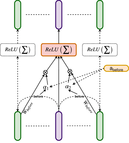
Figure 2: Attentive Graph Convolution (AT-GCN). In this layer, we learn attention weights for every edge based on label and direction. The attention weights are learnt using a context vector. The final representation of every node is a summation of weighted convolution over neighboring nodes based on labels.

Now, we compute the attention weight of node $j$ for node $i$ with respect to a direction-specific context vector $a_{L(i,j)}\in\mathbb{R}^{2F}$, as follows.

$$\alpha^{l(i,j)}_{ij}=\frac{\text{exp}\left(a_{L(i,j)}^{T}e_{ij}\right)}{\sum\limits_{k\in\mathcal{N}^{l(i,\cdot)}_{i}}\text{exp}\left(a_{L(i,j)}^{T}e_{ik}\right)},$$

where, $\alpha^{l(i,j)}_{ij}=0$ if node $i$ and $j$ is not connected through label $l$. $\mathcal{N}^{l(i,\cdot)}$ denotes the subset of the neighbourhood of node $i$ with label $l$ only. Please note that, although the linear transform weight ($W^{atten}_{L(i,j)}\in\mathbb{R}^{F\times k_{syn}}$) is specific to the coarse labels $L$, but for each finer label $l\in\mathcal{L}$ we get these convex weights of attentions. Figure 2 illustrates the above description w.r.t. edge type BEFORE.

Finally, the feature aggregation is done according to the attention weights. Prior to that, another label specific linear transformation is taken to perform the convolution operation. Then, the updated feature for node $i$ is calculated as follows.

where, $\alpha_{ii}=1$, $\ \mathcal{N}^{l(i,\cdot)}$ denotes the subset of the neighbourhood of node $i$ with label $l$ only. Note that, $\alpha^{l(i,j)}_{ij}=0$ when $j\notin\mathcal{N}^{l(i,\cdot)}$. To illustrate formally, from Figure 2, we see that weight $\alpha_{1}$ and $\alpha_{2}$ is calculated specific to label type BEFORE and the neighbours which are connected through BEFORE is being multiplied with $W_{before}$ prior to aggregation in the $ReLU$ block.

Now, after applying attentive graph convolution network, we only consider the representation of Document Creation Time (DCT), $h_{DCT}$, as the document representation itself. $h_{DCT}$ is now passed through a fully connected layer prior to softmax. Prediction of the OE-GCN for the document D will be given as

$$\mathrm{P}_{\mathrm{OE-GCN}}(y|D)=\mathrm{Softmax}(W\cdot d_{\mathrm{DCT}}+b).$$

4.3 AD3: Attentive Deep Document Dater

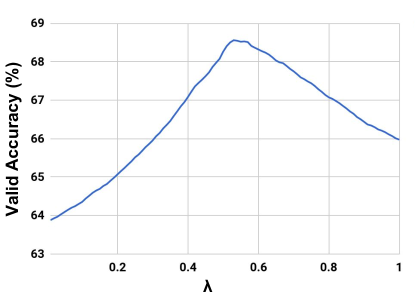
Figure 3: Variation of validation accuracy with $\lambda$ (for APW dataset). We observe that AC-GCN and OE-GCN are both important for the task as we get optimal $\lambda$ = 0.52.

In this section, we propose an unified model by mixing both AC-GCN and OE-GCN. Even on validation data, we see that performance of both the models differ to a large extent. This significant difference (McNemar test p $<$ 0.000001) motivated the unification. We take convex combination of the output probabilities of the two models as shown below.

$$$$\mathrm{P}_{joint}(y|D)=\lambda\mathrm{P}_{\mathrm{AC-GCN}}(y|D)\\ +(1-\lambda)\mathrm{P}_{\mathrm{OE-GCN}}(y|D)$$.$$

The combination hyper-parameter $\lambda$ is tuned on the validation data. We obtain the value of $\lambda$ to be 0.52 (Figure 3) and 0.54 for APW and NYT datasets, respectively. This depicts that the two models are capturing significantly different aspects of documents, resulting in a substantial improvement in performance when combined.

5 Experimental Setup

Datasets	# Docs	Start Year	End Year
APW	675k	1995	2010
NYT	647k	1987	1996

Table 1: Details of datasets used. Please refer Section 5 for details.

Dataset: Experiments are carried out on the Associated Press Worldstream (APW) and New York Times (NYT) sections of the Gigaword corpus Parker et al. (2011). We have used the same 8:1:1 split as Vashishth et al. (2018) for all the models. For quantitative details please refer to Table 1.

Evaluation Criteria: In accordance with prior work Chambers (2012); Kotsakos et al. (2014); Vashishth et al. (2018) the final task is to predict the publication year of the document. We give a brief description of the baselines below.

Baseline Methods:

• MaxEnt-Joint Chambers (2012): This method engineers several hand-crafted temporally influenced features to classify the document using MaxEnt Classifier.

• BurstySimDater Kotsakos et al. (2014): This is a purely statistical method which uses lexical similarity and term burstiness Lappas et al. (2009) for dating documents in arbitrary length time frame. For our experiments, we used a time frame length of 1 year.

• NeuralDater Vashishth et al. (2018): This is the first deep neural network based approach for the document dating task. Details are provided in Section 3.2.

Hyperparameters: We use 300-dimensional GloVe embeddings and 128-dimensional hidden state for both GCNs and BiLSTM with 0.8 dropout. We use Adam Kingma and Ba (2014) with 0.001 learning rate for training. For OE-GCN we use 2-layers of AT-GCN. 1-layer of S-GCN is used for both the models.

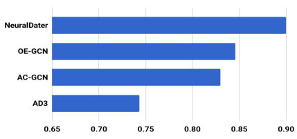
Figure 4: Mean absolute deviation (in years; lower is better) between a model’s top prediction and the true year in the APW dataset. We find that all of our proposed methods outperform the previous state-of-the-art NeuralDater. Please refer to Section 6.1 for details.

Method	APW	NYT
BurstySimDater	45.9	38.5
MaxEnt-Joint	52.5	42.5
NeuralDater	64.1	58.9
Attentive NeuralDater [6.2]	66.2	60.1
OE-GCN [4.2]	63.9	58.3
AC-GCN [4.1]	65.6	60.3
AD3 [4.3]	68.2	62.2

Table 2: Accuracy (%) of different methods on the APW and NYT datasets for the document dating problem (higher is better). The unified model significantly outperforms all previous models.

Method	Accuracy
T-GCN of NeuralDater	61.8
OE-GCN	63.9
S-GCN of NeuralDater	63.2
AC-GCN	65.6

Table 3: Accuracy (%) comparisons of component models with and without Attention. This results show the effectiveness of both word attention and Graph Attention for this task. Please see Section 6.2 for more details.

6 Results

6.1 Performance Analysis

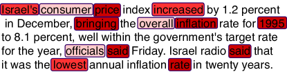
Figure 5: Visualization of the attention of AC-GCN. AC-GCN captures the intuitive tokens as seen in the figure. Darker shade implies higher attention. The correct DCT is 1996.

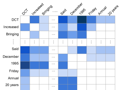
Figure 6: Visualization of the average edge attention of the temporal graph as learnt by OE-GCN for the document shown in Figure 5. Darker color implies higher attention. The correct DCT is 1996.

In this section, we compare the effectiveness of our method with that of prior work. The deep network based NeuralDater model in Vashishth et al. (2018) outperforms previous feature engineered Chambers (2012) and statistical methods Kotsakos et al. (2014) by a large margin. We observe a similar trend in our case. Compared to the state-of-the-art model NeuralDater, we gain, on an average, a 3.7% boost in accuracy on both the datasets (Table 2).

Among individual models, OE-GCN performs at par with NeuralDater, while AC-GCN outperforms it. The empirical results imply that AC-GCN by itself is effective for this task. The relatively worse performance of OE-GCN can be attributed to the fact that it only focuses on the Event-Time information and leaves out most of the contextual information. However, it captures various different (p $<$ 0.000001, McNemar’s test, 2-tailed) aspects of the document for classification, which motivated us to propose an ensemble of the two models. This explains the significant boost in performance of AD3 over NeuralDater as well as the individual models. It is worth mentioning that although AC-GCN and OE-GCN do not provide significant boosts in accuracy, their predictions have considerably lower mean-absolute-deviation as shown in Figure 4.

We concatenated the DCT embedding provided by OE-GCN with the document embedding provided by AC-GCN and trained in an end to end joint fashion like NeuralDater. We see that even with a similar training method, the Attentive NeuralDater model on an average, performs 1.6% better in terms of accuracy, once again proving the efficacy of attention based models over normal models.

6.2 Effectiveness of Attention

Attentive Graph Convolution (Section 4.2.2) proves to be effective for OE-GCN, giving a 2% accuracy improvement over non-attentive T-GCN of NeuralDater (Table 3). Similarly the efficacy of word level attention is also prominent from Table 3.
We have also analyzed our models by visualizing attentions over words and attention over graph nodes. Figure 5 shows that AC-GCN focuses on temporally informative words such as ”said” (for tense) or time mentions like “1995”, alongside important contextual words like “inflation”, “Israel” etc. For OE-GCN, from Figure 6 we observe that “DCT” and time-mention ‘1995’ grabs the highest attention. Attention between “DCT” and other event verbs indicating past tense are quite prominent, which helps the model to infer 1996 (which is correct) as the most likely time-stamp of the document. These analyses provide us with a good justification for the performance of our attentive models.

7 Discussion

Apart from empirical improvements over previous models, we also perform a qualitative analysis of the individual models. Figure 7 shows that the performance of AC-GCN improves with the length of documents, thus indicating that richer context leads to better model prediction. Figure 8 shows how the performance of OE-GCN improves with the number of event-time mentions in the document, thus further reinforcing our claim that more temporal information improves model performance.

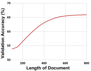
Figure 7: Variation of validation accuracy (%) with respect to length of documents (for APW dataset) for AC-GCN. Documents having more than 100 tokens are selected for this analysis. Please see Section 7.

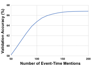
Figure 8: Variation of validation accuracy (%) with number of event-time mentions in documents (for APW dataset) for OE-GCN. Documents with more than 100 tokens are selected for this analysis. Please see Section 7.

Vashishth et al. (2018) reported that their model got confused by the presence of multiple misleading time mentions. AD3 overcomes this limitation using attentive graph convolution, which successfully filters out noisy time mentions as is evident from Figure 8.

8 Conclusion

We propose AD3, an ensemble model which exploits both syntactic and temporal information in a document explicitly to predict its creation time (DCT). To the best of our knowledge, this is the first application of attention based deep models for dating documents. Our experimental results demonstrate the effectiveness of our model over all previous models. We also visualize the attention weights to show that the model is able to choose what is important for the task and filter out noise inherent in language. As part of future work, we would like to incorporate external knowledge as a side information for improved time-stamping of documents.

References

- Allan et al. (1998) James Allan, Ron Papka, and Victor Lavrenko. 1998. On-line new event detection and tracking. In Proceedings of the 21st Annual International ACM SIGIR Conference on Research and Development in Information Retrieval, SIGIR ’98, pages 37–45, New York, NY, USA. ACM.
- Bahdanau et al. (2014) Dzmitry Bahdanau, Kyunghyun Cho, and Yoshua Bengio. 2014. Neural machine translation by jointly learning to align and translate. CoRR, abs/1409.0473.
- Bastings et al. (2017) Joost Bastings, Ivan Titov, Wilker Aziz, Diego Marcheggiani, and Khalil Sima’an. 2017. Graph convolutional encoders for syntax-aware neural machine translation. CoRR, abs/1704.04675.
- Chambers (2012) Nathanael Chambers. 2012. Labeling documents with timestamps: Learning from their time expressions. In Proceedings of the 50th Annual Meeting of the Association for Computational Linguistics: Long Papers - Volume 1, ACL ’12, pages 98–106, Stroudsburg, PA, USA. Association for Computational Linguistics.
- Dakka et al. (2008) Wisam Dakka, Luis Gravano, and Panagiotis G. Ipeirotis. 2008. Answering general time sensitive queries. In Proceedings of the 17th ACM Conference on Information and Knowledge Management, CIKM ’08, pages 1437–1438, New York, NY, USA. ACM.
- de Jong et al. (2005a) Franciska M.G. de Jong, H. Rode, and Djoerd Hiemstra. 2005a. Temporal Language Models for the Disclosure of Historical Text. KNAW. Imported from EWI/DB PMS [db-utwente:inpr:0000003683].
- de Jong et al. (2005b) Franciska M.G. de Jong, H. Rode, and Djoerd Hiemstra. 2005b. Temporal Language Models for the Disclosure of Historical Text. KNAW. Imported from EWI/DB PMS [db-utwente:inpr:0000003683].
- Hamilton et al. (2017) William L. Hamilton, Rex Ying, and Jure Leskovec. 2017. Inductive representation learning on large graphs. CoRR, abs/1706.02216.
- Kanhabua and Nørvåg (2008) Nattiya Kanhabua and Kjetil Nørvåg. 2008. Improving temporal language models for determining time of non-timestamped documents. In Proceedings of the 12th European Conference on Research and Advanced Technology for Digital Libraries, ECDL ’08, pages 358–370, Berlin, Heidelberg. Springer-Verlag.
- Kingma and Ba (2014) Diederik P. Kingma and Jimmy Ba. 2014. Adam: A method for stochastic optimization. CoRR, abs/1412.6980.
- Kipf and Welling (2016) Thomas N Kipf and Max Welling. 2016. Semi-supervised classification with graph convolutional networks. arXiv preprint arXiv:1609.02907.
- Kotsakos et al. (2014) Dimitrios Kotsakos, Theodoros Lappas, Dimitrios Kotzias, Dimitrios Gunopulos, Nattiya Kanhabua, and Kjetil Nørvåg. 2014. A burstiness-aware approach for document dating. In Proceedings of the 37th International ACM SIGIR Conference on Research & Development in Information Retrieval, SIGIR ’14, pages 1003–1006, New York, NY, USA. ACM.
- Lappas et al. (2009) Theodoros Lappas, Benjamin Arai, Manolis Platakis, Dimitrios Kotsakos, and Dimitrios Gunopulos. 2009. On burstiness-aware search for document sequences. In Proceedings of the 15th ACM SIGKDD International Conference on Knowledge Discovery and Data Mining, KDD ’09, pages 477–486, New York, NY, USA. ACM.
- Li and Croft (2003) Xiaoyan Li and W. Bruce Croft. 2003. Time-based language models. In Proceedings of the Twelfth International Conference on Information and Knowledge Management, CIKM ’03, pages 469–475, New York, NY, USA. ACM.
- Manning et al. (2014) Christopher D. Manning, Mihai Surdeanu, John Bauer, Jenny Finkel, Steven J. Bethard, and David McClosky. 2014. The Stanford CoreNLP natural language processing toolkit. In Association for Computational Linguistics (ACL) System Demonstrations, pages 55–60.
- Marcheggiani and Titov (2017) Diego Marcheggiani and Ivan Titov. 2017. Encoding sentences with graph convolutional networks for semantic role labeling. CoRR, abs/1703.04826.
- McDowell et al. (2017) Bill McDowell, Nathanael Chambers, Alexander Ororbia II, and David Reitter. 2017. Event ordering with a generalized model for sieve prediction ranking. In Proceedings of the Eighth International Joint Conference on Natural Language Processing (Volume 1: Long Papers), pages 843–853, Taipei, Taiwan. Asian Federation of Natural Language Processing.
- Mirza and Tonelli (2016) Paramita Mirza and Sara Tonelli. 2016. Catena: Causal and temporal relation extraction from natural language texts. In Proceedings of COLING 2016, the 26th International Conference on Computational Linguistics: Technical Papers, pages 64–75. The COLING 2016 Organizing Committee.
- Nguyen and Grishman (2018) Thien Huu Nguyen and Ralph Grishman. 2018. Graph convolutional networks with argument-aware pooling for event detection.
- Parker et al. (2011) Robert Parker, David Graff, Junbo Kong, Ke Chen, and Kazuaki Maeda. 2011. English gigaword fifth edition ldc2011t07. dvd. Philadelphia: Linguistic Data Consortium.
- Talukdar et al. (2012a) Partha Pratim Talukdar, Derry Wijaya, and Tom Mitchell. 2012a. Acquiring temporal constraints between relations. In Proceedings of the 21st ACM international conference on Information and knowledge management, pages 992–1001. ACM.
- Talukdar et al. (2012b) Partha Pratim Talukdar, Derry Wijaya, and Tom Mitchell. 2012b. Coupled temporal scoping of relational facts. In Proceedings of the fifth ACM international conference on Web search and data mining, pages 73–82. ACM.
- UzZaman et al. (2013) Naushad UzZaman, Hector Llorens, Leon Derczynski, James Allen, Marc Verhagen, and James Pustejovsky. 2013. Semeval-2013 task 1: Tempeval-3: Evaluating time expressions, events, and temporal relations. In Second Joint Conference on Lexical and Computational Semantics (* SEM), Volume 2: Proceedings of the Seventh International Workshop on Semantic Evaluation (SemEval 2013), volume 2, pages 1–9.
- Vashishth et al. (2018) Shikhar Vashishth, Shib Sankar Dasgupta, Swayambhu Nath Ray, and Partha Talukdar. 2018. Dating documents using graph convolution networks. In Proceedings of the 56th Annual Meeting of the Association for Computational Linguistics (Volume 1: Long Papers), pages 1605–1615. Association for Computational Linguistics.
- Vaswani et al. (2017) Ashish Vaswani, Noam Shazeer, Niki Parmar, Jakob Uszkoreit, Llion Jones, Aidan N Gomez, Ł ukasz Kaiser, and Illia Polosukhin. 2017. Attention is all you need. In I. Guyon, U. V. Luxburg, S. Bengio, H. Wallach, R. Fergus, S. Vishwanathan, and R. Garnett, editors, Advances in Neural Information Processing Systems 30, pages 5998–6008. Curran Associates, Inc.
- Veličković et al. (2018) Petar Veličković, Guillem Cucurull, Arantxa Casanova, Adriana Romero, Pietro Liò, and Yoshua Bengio. 2018. Graph attention networks. In International Conference on Learning Representations.
- Verhagen et al. (2010) Marc Verhagen, Roser Sauri, Tommaso Caselli, and James Pustejovsky. 2010. Semeval-2010 task 13: Tempeval-2. In Proceedings of the 5th international workshop on semantic evaluation, pages 57–62. Association for Computational Linguistics.
- Wan (2007) Xiaojun Wan. 2007. Timedtextrank: Adding the temporal dimension to multi-document summarization. In Proceedings of the 30th Annual International ACM SIGIR Conference on Research and Development in Information Retrieval, SIGIR ’07, pages 867–868, New York, NY, USA. ACM.
- Yang et al. (2016a) Zichao Yang, Xiaodong He, Jianfeng Gao, Li Deng, and Alexander J. Smola. 2016a. Stacked attention networks for image question answering. In 2016 IEEE Conference on Computer Vision and Pattern Recognition, CVPR 2016, Las Vegas, NV, USA, June 27-30, 2016, pages 21–29.
- Yang et al. (2016b) Zichao Yang, Diyi Yang, Chris Dyer, Xiaodong He, Alexander J. Smola, and Eduard H. Hovy. 2016b. Hierarchical attention networks for document classification. In NAACL HLT 2016, The 2016 Conference of the North American Chapter of the Association for Computational Linguistics: Human Language Technologies, San Diego California, USA, June 12-17, 2016, pages 1480–1489.