Chimera states in networks of locally and non-locally coupled SQUIDs

Abstract

Planar and linear arrays of SQUIDs (superconducting quantum interference devices), operate as nonlinear magnetic metamaterials in microwaves. Such SQUID metamaterials are paradigmatic systems that serve as a test-bed for simulating several nonlinear dynamics phenomena. SQUIDs are highly nonlinear oscillators which are coupled together through magnetic dipole-dipole forces due to their mutual inductance; that coupling falls-off approximately as the inverse cube of their distance, i. e., it is non-local. However, it can be approximated by a local (nearest-neighbor) coupling which in many cases suffices for capturing the essentials of the dynamics of SQUID metamaterials. For either type of coupling, it is numerically demonstrated that chimera states as well as other spatially non-uniform states can be generated in SQUID metamaterials under time-dependent applied magnetic flux for appropriately chosen initial conditions. The mechanism for the emergence of these states is discussed in terms of the multistability property of the individual SQUIDs around their resonance frequency and the attractor crowding effect in systems of coupled nonlinear oscillators. Interestingly, generation and control of chimera states in SQUID metamaterials can be achieved in the presence of a constant (dc) flux gradient with the SQUID metamaterial initially at rest.

I Introduction

The notion of metamaterials refers to artificially structured media designed to achieve properties not available in natural materials. Originally they were comprising subwavelength resonant elements, such as the celebrated split-ring resonator (SRR). The latter, in its simplest version, is just a highly conducting metallic ring with a slit, that can be regarded as an effectively resistive - inductive - capacitive ($RLC$) electrical circuit. There has been a tremendous amount of activity in the field of metamaterials the last two decades, the results of which have been summarized in a number of review articles Smith et al. (2004); Linden et al. (2006); Padilla et al. (2006); Shalaev (2007); Litchinitser and Shalaev (2008); Soukoulis and Wegener (2011); Liu and Zhang (2011); Simovski et al. (2012) and books Engheta and Ziokowski (2006); Pendry (2007); Ramakrishna and Grzegorczyk (2009); Cui et al. (2010); Cai and Shalaev (2010); Solymar and Shamonina (2009); Noginov and Podolskiy (2012); Tong (2018). One of metamaterial’s most remarkable properties is that of the negative refraction index, which results from simultaneously negative dielectric permittivity and diamagnetic permeability.

An important subclass of metamaterials is that of superconducting ones Anlage (2011); Jung et al. (2014a), in which the elementary units (i. e., the SRRs) are made by a superconducting material, typically Niobium ($Nb$) Jin et al. (2010) or Niobium Nitride ($NbN$) Zhang et al. (2012), as well as perovskite superconductors such as yttrium barium copper oxide ($YBCO$) Gu et al. (2010). In superconductors, the dc resistance vanishes below a critical temperature $T_{c}$; thus, below $T_{c}$, superconducting metamaterials have the advantage of ultra-low losses, a highly desirable feature for prospective applications. Moreover, when they are in the superconducting state, these metamaterials exhibit extreme sensitivity in external stimuli such as the temperature and magnetic fields, which makes their thermal and magnetic tunability possible Zhang et al. (2014). Going a step beyond, the superconducting SRRs can be replaced by SQUIDs Du et al. (2006); Lazarides and Tsironis (2007), where the acronym stands for Superconducting QUantum Interference Devices. The simplest version of such a device consists of a superconducting ring interrupted by a Josephson junction (JJ) Josephson (1962), as shown schematically in Fig. 1(a); the most common type of a JJ is formed whenever two superconductors are separated by a thin insulating layer (superconductor / insulator / superconductor JJ). The current through the insulating layer and the voltage across the JJ are then determined by the celebrated Josephson relations. Through these relations, the JJ provides a strong and well-studied nonlinearity to the SQUID, which makes the latter a unique nonlinear oscillator that can be actually manipulated through multiple external means.

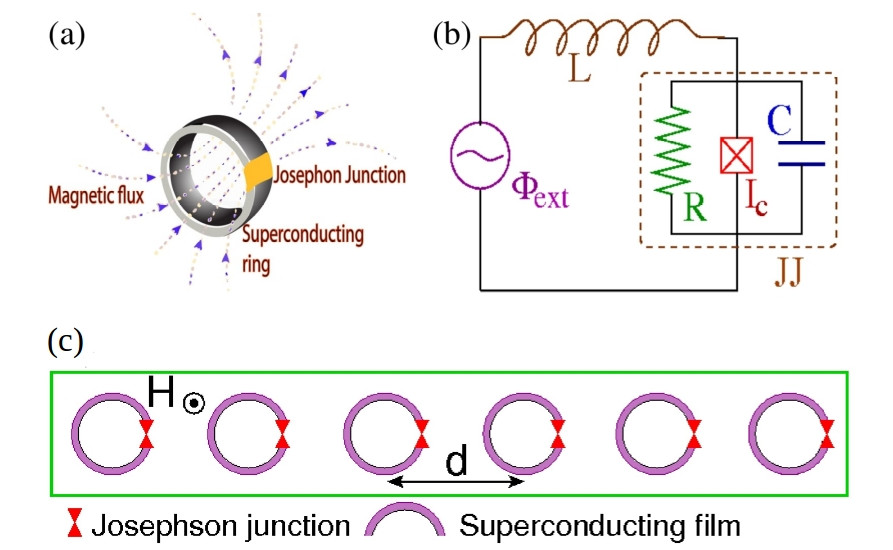
Figure 1: (a) Schematic of a SQUID (superconducting quantum interference device) in a magnetic field. (b) Equivalent electrical circuit. (c) Schematic top view of a one-dimensional periodic array of SQUIDs in a magnetic field $\bf H$

SQUID metamaterials are extended systems containing a large number of SQUIDs arranged in various configurations which, from the dynamical systems point of view, can be viewed theoretically as an assembly of weakly coupled nonlinear oscillators that inherit the flexibility of their constituting elements (i.e, the SQUIDs). They present a nonlinear dynamics laboratory in which numerous classical as well as quantum complex spatio-temporal phenomena can be explored. Recent experiments on SQUID metamaterials have revealed several extraordinary properties such as negative permeability Butz et al. (2013), broad-band tunability Butz et al. (2013); Trepanier et al. (2013), self-induced broad-band transparency Zhang et al. (2015), dynamic multistability and switching Jung et al. (2014b), as well as coherent oscillations Trepanier et al. (2017). Moreover, nonlinear effects such as localization of the discrete breather type Lazarides et al. (2008) and nonlinear band-opening (nonlinear transmission) Tsironis et al. (2014), as well as the emergence of counter-intuitive dynamic states referred to as chimera states in current literature Lazarides et al. (2015); Hizanidis et al. (2016a, b), have been demonstrated numerically in SQUID metamaterial models Lazarides and Tsironis (2018a).

The chimera states, in particular, which were first discovered in rings of non-locally and symmetrically coupled identical phase oscillators Kuramoto and Battogtokh (2002), have been reviewed thoroughly in recent articles Panaggio and Abrams (2015); Schöll (2016); Yao and Zheng (2016), are characterized by the coexistence of synchronous and asynchronous clusters of oscillators; their discovery was followed by intense theoretical Abrams and Strogatz (2004); Kuramoto et al. (2006); Omel’chenko et al. (2008); Abrams et al. (2008); Pikovsky and Rosenblum (2008); Ott and Antonsen (2009); Martens et al. (2010); Omelchenko et al. (2011); Yao et al. (2013); Omelchenko et al. (2013); Hizanidis et al. (2014); Zakharova et al. (2014); Bountis et al. (2014); Yeldesbay et al. (2014); Haugland et al. (2015); Bera et al. (2016); Shena et al. (2017); Sawicki et al. (2017); Ghosh and Jalan (2018); Shepelev and Vadivasova (2018); Banerjee and Sikder (2018) and experimental Tinsley et al. (2012); Hagerstrom et al. (2012); Wickramasinghe and Kiss (2013); Nkomo et al. (2013); Martens et al. (2013); Schönleber et al. (2014); Viktorov et al. (2014); Rosin et al. (2014); Schmidt et al. (2014); Gambuzza et al. (2014); Kapitaniak et al. (2014); Larger et al. (2015); Hart et al. (2016); English et al. (2017); Totz et al. (2018) activities, in which chimera states have been observed experimentally or demonstrated numerically in a huge variety of physical and chemical systems.

Here, the possibility for generating chimera states in SQUID metamaterials driven by a time-dependent magnetic flux by proper initialization or by the application of a dc flux gradient is demonstrated numerically. The SQUIDs in such a metamaterial are coupled together through magnetic dipole-dipole forces due to their mutual inductance. This kind of coupling between SQUIDs falls-off approximately as the inverse cube of their center-to-center distance, and thus it is clearly non-local. However, due to the magnetic nature of the coupling, its strength is weak Trepanier et al. (2013, 2017), and thus a nearest-neighbor coupling approach (i. e., a local coupling approach) is often sufficient in capturing the essentials of the dynamics of SQUID metamaterials. Chimera states emerge in SQUID metamaterials with either non-local Lazarides et al. (2015); Hizanidis et al. (2016b) or local Hizanidis et al. (2016a) coupling between SQUIDs. They can be generated from a large variety of initial conditions, and they are characterized using well-established measures. It is also demonstrated that chimera states emerge in SQUID metamaterials with zero initial conditions using a dc flux gradient; in that case, control over the obtained chimera states can be achieved.

In the next section, a model for a single SQUID that relies on the equivalent electrical circuit of Fig. 1(b) is described, and the dynamic equation for the flux through the ring of the SQUID is derived and normalized. In Section 3, the dynamic equations for a one-dimensional (1D) SQUID metamaterial with non-local coupling are derived, and subsequently they are reduced to the local coupling limit. In Section 4, various types of chimera states are presented and characterized using appropriate measures. In Section 5, the possibility to generate and control chimera states with a dc flux gradient, is explored. A brief discussion and conclusions are presented in Section 6.

II The SQUID oscillator

The simplest version of a SQUID consists of a superconducting ring interrupted by a JJ (Fig. 1(a)), which can be modeled by the equivalent electrical circuit of Fig. 1(b); according to that model, the SQUID features a self-inductance $L$, a capacitance $C$, a resistance $R$, and a critical current $I_{c}$ which characterizes an ideal JJ. A “real” JJ (brown-dashed square in Fig. 1(b)) is however modeled as a parallel combination of an ideal JJ, the resistance $R$, and the capacitance $C$. When a time-dependent magnetic field is applied to the SQUID in a direction transverse to its ring, the flux threading the SQUID ring induces two types of currents; the supercurrent, which is lossless, and the so-called quasiparticle current which is subject to Ohmic losses. The latter roughly corresponds to the current through the branch containing the resistor $R$ in Fig. 1(b). The (generally time-dependent) flux threading the ring of the SQUID is described in the model as a flux source, $\Phi_{ext}$. Many variants of SQUIDs have been studied for several decades (since 1964) and they have found numerous applications in magnetic field sensors, biomagnetism, non-destructive evaluation, and gradiometers, among others Clarke and Braginski (2004a, b). SQUIDs exhibit very rich dynamics including multistability, complex bifurcation structure, and chaotic behavior Hizanidis et al. (2018).

The magnetic flux $\Phi$ threading the ring of the SQUID is given by

$$\Phi=\Phi_{ext}+L\,I,$$ (1)

where $\Phi_{ext}$ is the external flux applied to the SQUID, and

$$I=-C\frac{d^{2}\Phi}{dt^{2}}-\frac{1}{R}\frac{d\Phi}{dt}-I_{c}\,\sin\left(2\pi\frac{\Phi}{\Phi_{0}}\right),$$ (2)

is the total current induced in the SQUID as provided by the resistively and capacitively shunted junction (RCSJ) model of the JJ Likharev. (1986) (the part of the circuit in Fig. 1(b) contained in the brown-dashed square), $\Phi_{0}$ is the flux quantum, and $t$ is the temporal variable. The three terms in the right-hand-side of Eq. (1) correspond to the current through the capacitor $C$, the current through the resistor $R$, and the supercurrent through the ideal JJ, respectively. The combination of Eqs. (1) and (2) gives

$$C\frac{d^{2}\Phi}{dt^{2}}+\frac{1}{R}\frac{d\Phi}{dt}+I_{c}\,\sin\left(2\pi\frac{\Phi}{\Phi_{0}}\right)+\frac{\Phi-\Phi_{ext}}{L}=0.$$ (3)

Note that losses decrease with increasing Ohmic resistance $R$, which is a peculiarity of the SQUID device. The external flux usually consists of a constant (dc) term $\Phi_{dc}$ and a sinusoidal (ac) term of amplitude $\Phi_{ac}$ and frequency $\Omega$, i. e., it is of the form

$$\Phi_{ext}=\Phi_{dc}+\Phi_{ac}\,\cos(\omega t).$$ (4)

The normalized form of Eq. (3) be obtained by using the relations

$$\phi=\frac{\Phi}{\Phi_{0}},~{}~{}~{}\phi_{ac,dc}=\frac{\Phi_{ac,dc}}{\Phi_{0}},~{}~{}~{}\tau=\frac{t}{\omega_{LC}^{-1}},~{}~{}~{}\Omega=\frac{\omega}{\omega_{LC}},$$ (5)

where $\omega_{LC}=1/\sqrt{LC}$ is the inductive-capacitive ($L\,C$) SQUID frequency (geometrical frequency), and the definitions

$$\beta=\frac{I_{c}L}{\Phi_{0}}=\frac{\beta_{L}}{2\pi},\qquad\gamma=\frac{1}{R}\sqrt{\frac{L}{C}}.$$ (6)

for the rescaled SQUID parameter and the loss coefficient, respectively. Thus we get

$$\ddot{\phi}+\gamma\dot{\phi}+\phi+\beta\sin\left(2\pi\phi\right)=\phi_{dc}+\phi_{ac}\cos(\Omega\tau).$$ (7)

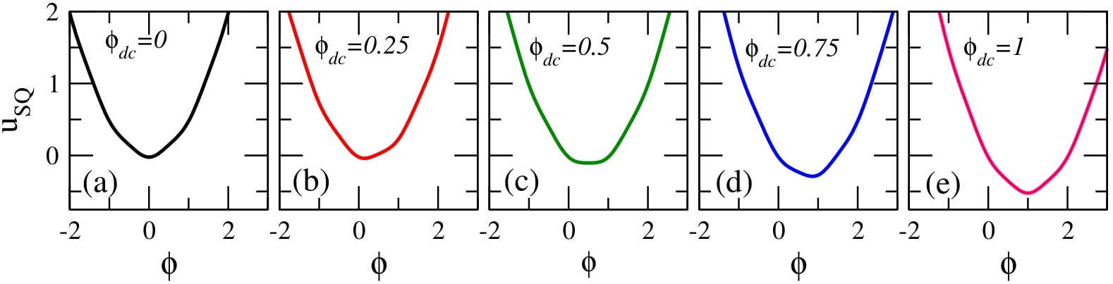
Figure 2: SQUID potential curves $u_{SQ}(\phi)$ for $\beta_{L}=0.86$, $\phi_{ac}=0$, and (a) $\phi_{dc}=0$; (b) $\phi_{dc}=0.25$; (c) $\phi_{dc}=0.5$; (d) $\phi_{dc}=0.75$; (e) $\phi_{dc}=1.0$.

By substituting $\gamma=0$ and $\phi_{ext}=0$ and $\beta\sin\left(2\pi\phi\right)\simeq\beta_{L}\phi$ into Eq. (7), we get $\ddot{\phi}+\Omega_{SQ}^{2}\phi=0$, with $\Omega_{SQ}=\sqrt{1+\beta_{L}}$ being the linear eigenfrequency (resonance frequency) of the SQUID. Eq. (7) can be also written as

$$\ddot{\phi}+\gamma\dot{\phi}=-\frac{du_{SQ}}{d\phi},$$ (8)

where

$$u_{SQ}=-\phi_{ext}(\tau)\phi+\frac{1}{2}\left[\phi^{2}-\frac{\beta}{\pi}\cos(2\pi\phi)\right],$$ (9)

is the normalized SQUID potential, and

$$\phi_{ext}(\tau)=\phi_{dc}+\phi_{ac}\cos(\Omega\tau),$$ (10)

is the normalized external flux. The SQUID potential $u_{SQ}$ given by Eq. (9) is time-dependent for $\phi_{ac}\neq 0$ and $\Omega\neq 0$. Here, parameter values of $\beta_{L}$ less than unity ($\beta_{L}<1$) are considered, in accordance with recent experiments; in that case, $u_{SQ}$ is a single-well, although nonlinear potential. For $\phi_{ext}=\phi_{dc}$, there is no time-dependence; however, the shape of $u_{SQ}$ varies with varying $\phi_{dc}$, as it can be seen in Fig. 2. The potential $u_{SQ}$ is symmetric around a particular $\phi$ for integer and half-integer values of $\phi_{dc}$. (In Figs. 2(a), (c), and (e), the potential $u_{SQ}$ is symmetric around $\phi=0$, $0.5$, and $1$, respectively.) For all the other values of $\phi_{dc}$, the potential $u_{SQ}$ is asymmetric; this asymmetry of $u_{SQ}$ allows for chaotic behavior to appear in an ac and dc driven single SQUID through period-doubling bifurcation cascades. Such cascades and the subsequent transition to chaos are prevented by a symmetric $u_{SQ}$ which renders the SQUID a symmetric system in which period-doubling bifurcations are suppressed Swift and Wiesenfeld (1984). Actually, suppression of period-doubling bifurcation cascades due to symmetry occurs in a large class of systems, including the sinusoidally driven-damped pendulum.

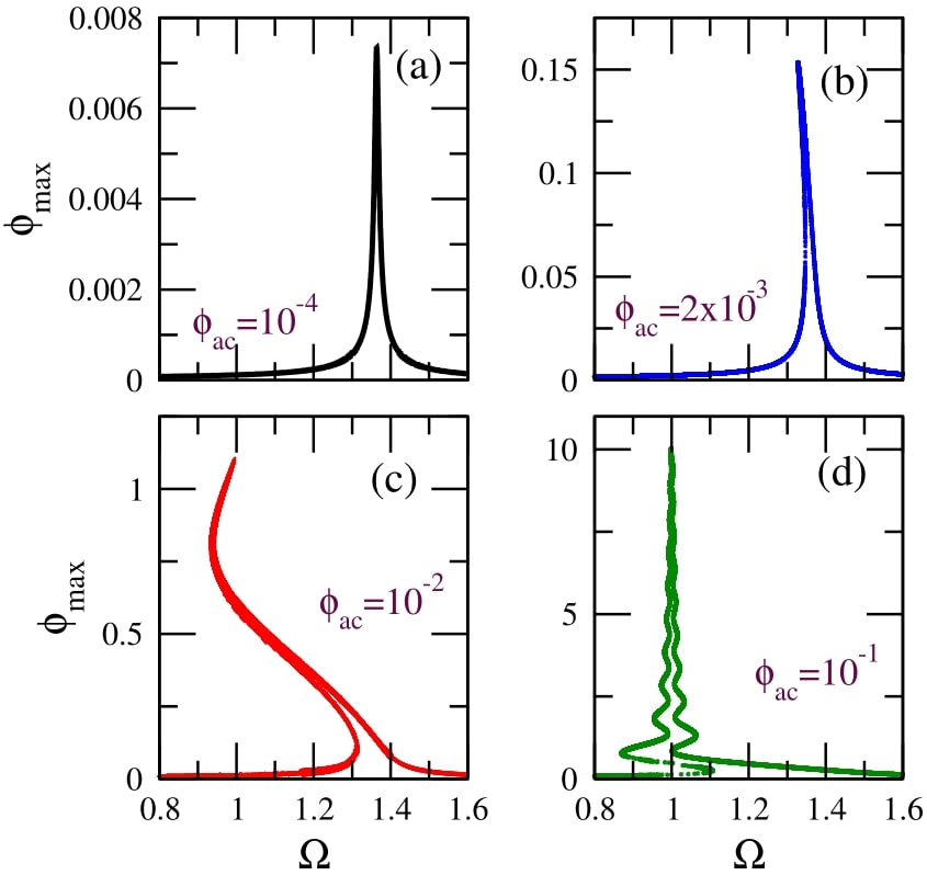
Figure 3: Flux amplitude - driving frequency ($\phi_{max}-\Omega$) curves for a SQUID with $\beta_{L}=0.86$, $\gamma=0.01$, $\phi_{dc}=0$, and (a) $\phi_{ac}=10^{-4}$, (b) $\phi_{ac}=2\times 10^{-3}$, (c) $\phi_{ac}=10^{-2}$, (d) $\phi_{ac}=10^{-1}$.

For zero dc flux, the strength of the SQUID nonlinearity increases with increasing ac flux amplitude $\phi_{ac}$. This effect is illustrated in Fig. 3 in which the flux amplitude - driving frequency ($\phi_{max}-\Omega$) curves, i. e., the resonance curves, for four values of $\phi_{ac}$ spanning four orders of magnitude are shown (for $\phi_{dc}=0$). In Fig. 3(a), for $\phi_{ac}=0.0001$, the SQUID is in the linear regime and thus its $\phi_{max}-\Omega$ curve is apparently symmetric around the linear SQUID eigenfrequency, $\Omega_{SQ}=\sqrt{1+\beta_{L}}\simeq 1.364$. Weak nonlinear effects begin to appear in Fig. 3(b), for $\phi_{ac}=0.002$, in which the curve is slightly bended to the left. In Fig. 3(c), for $\phi_{ac}=0.01$, the nonlinear effects are already strong enough to generate a multistable $\phi_{max}-\Omega$ curve. In Fig. 3(d), for $\phi_{ac}=0.1$, the SQUID is in the strongly nonlinear regime and the $\phi_{max}-\Omega$ curve has acquired a snake-like form. Indeed, the curve “snakes” back and forth within a narrow frequency region via successive saddle-node bifurcations Hizanidis et al. (2018). Note that in Figs. 3(c) and (d), the frequency region with the highest multistability is located around the geometrical frequency of the SQUID, i. e., at $\Omega\simeq 1$ (the $L\,C$ frequency in normalized units). Inasmuch the frequency at which $\phi_{max}$ is highest can be identified with the “resonance” frequency of the SQUID, it can be observed that this resonance frequency lowers with increasing $\phi_{ac}$ from the linear SQUID eigenfrequency $\Omega_{SQ}$ to the inductive-capacitive (geometrical) frequency $\Omega\simeq 1$. Thus, the resonance frequency of the SQUID, where its multistability is highest, can be actually tuned by nonlinearity, i. e., by varying the ac flux amplitude $\phi_{ac}$. Note that the multistability of the SQUID is a purely dynamic effect, which is not related to any local minima of the SQUID potential (which is actually single-welled for the values of $\beta_{L}$ considered here, i. e., for $\beta_{L}<1$).

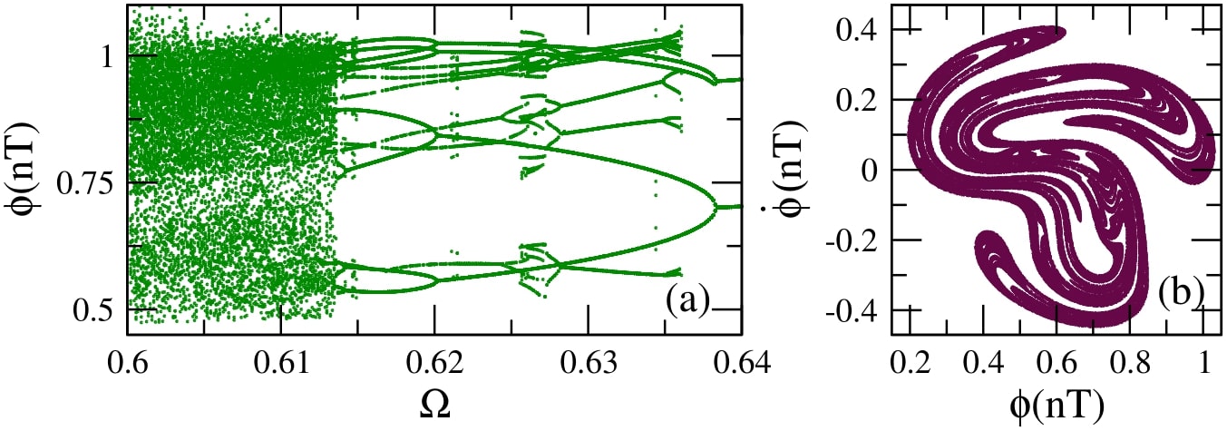
Figure 4: (a) Bifurcation diagram of $\phi(nT)$ as a function of the driving frequency $\Omega$, for $\beta_{L}=0.86$, $\gamma=0.01$, $\phi_{dc}=0.36$, and $\phi_{ac}=0.18$. (b) A typical chaotic attractor on the $\phi-\dot{\phi}$ phase-plane for $\Omega=0.6$. The other parameters are as in (a).

For $\phi_{dc}\neq 0$, chaotic behavior appears in wide frequency intervals below the geometrical frequency ($\Omega=1$) for relatively high $\phi_{ac}$. As it was mentioned above, the SQUID potential $u_{SQ}$ is asymmetric for $\phi_{dc}\neq 0$, and thus the SQUID can make transitions to chaos through period-doubling cascades Hizanidis et al. (2018). In the bifurcation diagram shown in Fig. 4(a), the flux $\phi$ is plotted at the end of each driving period $T=2\pi/\Omega$ for several tenths of driving periods (transients have been rejected) as a function of the driving frequency $\Omega$. This bifurcation diagram reveals multistability as well as a reverse period-doubling cascade leading to chaos. That reverse cascade, specifically, begins at $\Omega=0.64$ with a stable period-2 solution (i. e., whose period is two times that of the driving period $T$). A period-doubling occurs at $\Omega=0.638$ resulting in a stable period-4 solution. The next period-doubling, at $\Omega=0.62$, results in a stable period-8 solution. The last period-doubling bifurcation which is visible in this scale occurs at $\Omega=0.614$ and results in a stable period-16 solution. More and more period-doubling bifurcations very close to each other lead eventually to chaos at $\Omega=0.6132$. Note that another stable multiperiodic solution is present in the frequency interval shown in Fig. 4(a). A typical chaotic attractor of the SQUID is shown on the $\phi-\dot{\phi}$ phase plane in Fig. 4(b) for $\Omega=0.6$.

III SQUID metamaterials: Modelling

III.1 Flux dynamics equations

Consider a one-dimensional periodic arrangement of $N$ identical SQUIDs in a transverse magnetic field $\bf H$ as in Fig. 1(c), which center-to-center distance is $d$ and they are coupled through (non-local) magnetic dipole-dipole forces Lazarides et al. (2015). The magnetic flux $\Phi_{n}$ threading the ring of the $n-$th SQUID is

$$\Phi_{n}=\Phi_{ext}+L\,I_{n}+L\,\sum_{m\neq n}\lambda_{|m-n|}I_{m},$$ (11)

where $n,m=1,...,N$, $\Phi_{ext}$ is the external flux in each SQUID, $\lambda_{|m-n|}=M_{|m-n|}/L$ is the dimensionless coupling coefficient between the SQUIDs at the sites $m$ and $n$, with $M_{|m-n|}$ being their mutual inductance, and

$$-I_{n}=C\frac{d^{2}\Phi_{n}}{dt^{2}}+\frac{1}{R}\frac{d\Phi_{n}}{dt}+I_{c}\,\sin\left(2\pi\frac{\Phi_{n}}{\Phi_{0}}\right)$$ (12)

is the current in the $n-$th SQUID as given by the RCSJ model Likharev. (1986). The combination of Eqs. (11) and (12) gives

$$C\frac{d^{2}\Phi_{n}}{dt^{2}}+\frac{1}{R}\frac{d\Phi_{n}}{dt}+I_{c}\,\sin\left(2\pi\frac{\Phi_{n}}{\Phi_{0}}\right)$$

$$+\frac{1}{L}\sum_{m=1}^{N}\left({\bf\hat{\Lambda}}^{-1}\right)_{nm}\left(\Phi_{m}-\Phi_{ext}\right)=0,$$ (13)

where ${\bf\hat{\Lambda}}^{-1}$ is the inverse of the symmetric $N\times N$ coupling matrix with elements

$${\bf\hat{\Lambda}}_{nm}=\left\{\begin{array}[]{ll}1,&\mbox{if $m=n$};\\ \lambda_{|m-n|}=\lambda_{1}\,|m-n|^{-3},&\mbox{if $m\neq n$},\end{array}\right.$$ (16)

with $\lambda_{1}$ being the coupling coefficient betwen nearest neighboring SQUIDs. In normalized form Eq. (III.1) reads ($n=1,...,N$)

$$\ddot{\phi}_{n}+\gamma\dot{\phi}_{n}+\beta\sin\left(2\pi\phi_{n}\right)=\sum_{m=1}^{N}\left({\bf\hat{\Lambda}}^{-1}\right)_{nm}\left(\phi_{ext}-\phi_{m}\right),$$ (17)

where Eq. (5) and the definitions Eq. (6) have been used. When nearest-neighbor coupling is only taken into account, Eq. (17) reduces to the simpler form

$$\ddot{\phi}_{n}+\gamma\dot{\phi}_{n}+\phi_{n}+\beta\sin\left(2\pi\phi_{n}\right)=\lambda(\phi_{n-1}+\phi_{n+1})$$

$$+(1-2\lambda)\phi_{ext},$$ (18)

where $\lambda=\lambda_{1}$.

III.2 Local and nonlocal linear frequency dispersion

Equation (11) with $\Phi_{ext}=0$ can be written in matrix form as

$$L\,{\bf\hat{\Lambda}}\vec{I}=\vec{\Phi},$$ (19)

where the elements of the coupling matrix ${\bf\hat{\Lambda}}$ are given in Eq. (16), and $\vec{I}$, $\vec{\Phi}$ are $N-$dimensional vectors with components $I_{n}$, $\Phi_{n}$, respectively. The linearized equation for the current in the $n-$th SQUID, in the lossless case ($R\rightarrow\infty$), is given from Eq. (12) as

$$-\vec{I}=C\frac{d^{2}}{dt^{2}}\vec{\Phi}+2\pi\frac{I_{c}}{\Phi_{0}}\vec{\Phi},$$ (20)

where the approximation $\sin(x)\simeq x$ has been employed. By substituting Eq. (20) into Eq. (19), we get

$${\bf\hat{\Lambda}}\left(\frac{1}{\omega_{LC}^{2}}\frac{d^{2}}{dt^{2}}\vec{\Phi}+\beta_{L}\vec{\Phi}\right)+\vec{\Phi}=0.$$ (21)

In component form, the corresponding equation reads

$$\sum_{m}{\bf\hat{\Lambda}}_{nm}\left(\frac{1}{\omega_{LC}^{2}}\frac{d^{2}}{dt^{2}}\Phi_{m}+\beta_{L}\Phi_{m}\right)+\Phi_{n}=0,$$ (22)

or, in normalized form

$$\sum_{m}{\bf\hat{\Lambda}}_{nm}\left(\frac{1}{\omega_{LC}^{2}}\ddot{\phi}_{m}+\beta_{L}\phi_{m}\right)+\phi_{n}=0,$$ (23)

where the overdots denote derivation with respect to the normalized time $\tau$.

Substitute the trial (plane wave) solution

$$\phi_{n}=\exp^{i(\kappa n-\Omega\tau)},$$ (24)

where $\kappa$ is the dimensionless wavenumber (in units of $d^{-1}$), into Eq. (23) to obtain

$$\Omega^{2}=\frac{1}{S}\left(1+\beta_{L}S\right),$$ (25)

where

$$S=\sum_{m}{\bf\hat{\Lambda}}_{nm}\exp^{i\kappa(m-n)}.$$ (26)

It can be shown that, for the infinite system, the funcion $S$ is

$$S=1+2\lambda\sum_{s=1}^{\infty}\frac{\cos(\kappa s)}{|s|^{3}}=1+2\lambda Ci_{3}(\kappa),$$ (27)

where $s=m-n$, and $Ci_{3}(\kappa)$ is a Clausen function. Putting Eq. (27) into Eq. (25), we obtain the nonlocal frequency dispersion for the 1D SQUID metamaterial as

$$\Omega_{\kappa}=\sqrt{\frac{\Omega_{SQ}^{2}+2\lambda\beta_{L}Ci_{3}(\kappa)}{1+2\lambda Ci_{3}(\kappa)}},$$ (28)

where $\Omega_{SQ}^{2}=1+\beta_{L}$. In the case of local (nearest-neighbor) coupling the Clausen function $Ci_{3}(\kappa)$ is replaced by $\cos(\kappa)$. Then, by neglecting terms of order $\lambda^{2}$ or higher, the local frequency dispersion

$$\Omega_{\kappa}\simeq\sqrt{\Omega_{SQ}^{2}-2\lambda\cos(\kappa)}$$ (29)

is obtained.

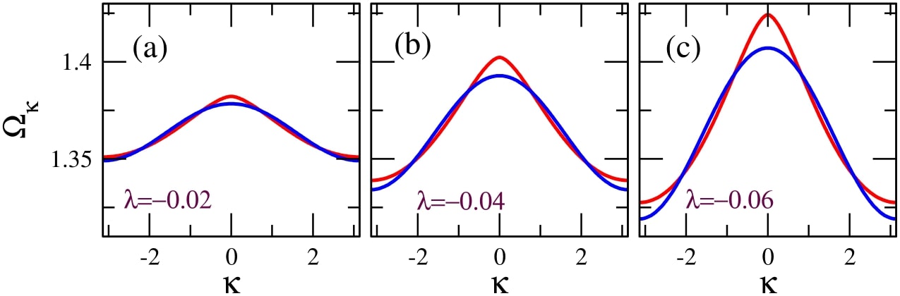
Figure 5: Linear frequency dispersion $\Omega=\Omega_{\kappa}$ for nonlocal (red) and local (blue) coupling, for $\beta_{L}=0.86$, and (a) $\lambda=-0.02$, (b) $\lambda=-0.04$; (c) $\lambda=-0.06$.

The linear frequency dispersion $\Omega=\Omega_{\kappa}$, calculated for nonlocal and local coupling from Eq. (28) and (29), respectively, is plotted in Fig. 5 for three values of the coupling coefficient $\lambda$. The differences between the nonlocal and local dispersion are rather small, especially for low values of $\lambda$, i. e., for $\lambda=-0.02$ (Fig. 5(a)), which are mostly considered here. Although the linear frequency bands are narrow, the bandwidth $\Delta\Omega=\Omega_{max}-\Omega_{min}$ increases with increasing $\lambda$. For simplicity, the bandwidth $\Delta\Omega$ can be estimated from Eq. (29); from that equation the minimum and maximum frequencies of the band can be approximated by $\Omega_{min,max}\simeq\Omega_{SQ}\left(1\pm\frac{\lambda}{\Omega_{SQ}^{2}}\right)$, so that

$$\Delta\Omega\simeq\frac{2|\lambda|}{\Omega_{SQ}}.$$ (30)

That is, the bandwidth is roughly proportional to the magnitude of $\lambda$. Note that for physically relevant parameters, the minimum frequency of the linear band is well above the geometrical (i. e., inductive-capacitive) frequency of the SQUIDs in the metamaterial. Thus, for strong nonlinearity, for which the resonance frequency of the SQUIDs is close to the geometrical one ($\Omega=1$), no plane waves can be excited. It is this frequency region where localized and other spatially inhomogeneous states such as chimera states are expected to emerge (given also the extreme multistability of individual SQUIDs there).

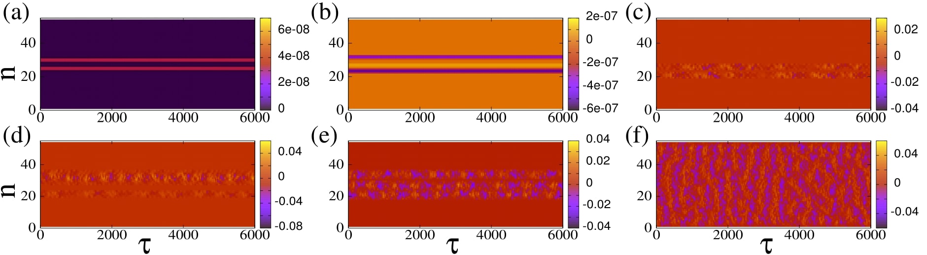
Figure 6: Maps of $\langle\dot{\phi}_{n}\rangle(\tau)$ on the $n-\tau$ plane for $\beta_{L}=0.86$, $\gamma=0.01$, $\lambda=-0.02$, $\Omega=1.01$, $N=54$, $\phi_{dc}=0$, and (a) $\phi_{ac}=0.02$, (b) $\phi_{ac}=0.04$, (c) $\phi_{ac}=0.06$, (d) $\phi_{ac}=0.08$, (e) $\phi_{ac}=0.10$, (f) $\phi_{ac}=0.12$.

IV Chimeras and other spatially inhomogeneous states

Eqs. (17) are integrated numerically in time with free-end boundary conditions ($\phi_{N+1}=\phi_{0}=0$) using a fourth-order Runge-Kutta algorithm with time-step $h=0.02$. The initial conditions have been chosen so that they lead to chimera states. It should be noted that chimera states can be obtained from a huge variety of initial conditions. Here we choose

$$\phi_{n}(\tau=0) = \left\{\begin{array}[]{ll}1,&\mbox{for $n_{\ell}<n\leq n_{r}$};\\ 0,&\mbox{otherwise},\end{array}\right.$$ (33)

$$\qquad\dot{\phi}_{n}(\tau=0) = 0,$$ (34)

with $n_{\ell}=18$ and $n_{r}=36$. Eqs. (17) are first integrated in time for a relatively long time-interval, $10^{7}~{}T$ time-units, where $T=2\pi/\Omega$ is the driving period, so that the system has reached a steady-state. While the SQUID metamaterial is in the steady-state, Eqs. (17) are integrated for $\tau_{sst}=1000~{}T$ more time-units. Then, the profiles of the time-derivatives of the fluxes, averaged over the driving period $T$, i. e.,

$${\langle\dot{\phi}_{n}\rangle}_{T}=\frac{1}{T}\int_{0}^{T}\dot{\phi}_{n}\,d\tau,~{}~{}~{}~{}n=1,...,N,$$ (35)

are mapped as a function of $\tau$. Such maps are shown in Fig. 6, for several values of the ac flux amplitude, $\phi_{ac}$. In these maps, areas with uniform colorization indicate that the SQUID oscillators there are synchronized, while areas with non-uniform colorization indicate that they are desynchronized.

In Figs. 6(a) and (b), i. e., for low values of $\phi_{ac}$, chimera states are not excited since the ${\langle\dot{\phi}_{n}\rangle}_{T}$ are practically zero during the steady-state integration time. However, this does not mean that the state of the SQUID metamaterial is spatially homogeneous, as we shall see below. For higher values of $\phi_{ac}$, chimera states begin to appear, in which one or more desynchronized clusters of SQUID oscillators roughly in the middle of the SQUID metamaterial are visible (Figs. 6(c)-(e)). For even higher values of $\phi_{ac}$, as can be seen in Fig. 6(f), the whole SQUID metamaterial is desynchronized. In order to quantify the degree of synchronization for SQUID metamaterials at a particular time-instant $\tau$, the magnitude of the complex synchronization (Kuramoto) parameter $r$ is calculated, where

$$r(\tau)=\left|\Psi(\tau)\right|=\frac{1}{N}\left|\sum_{n}e^{2\pi i\phi_{n}(\tau)}\right|.$$ (36)

Below, two averages of $r(\tau)$ are used for the characterization of a particular state of SQUID metamaterials, i. e., the average of $r(\tau)$ over the driving period $T$, ${\langle r\rangle}_{T}(\tau)$, and the average of $r(\tau)$ over the steady-state integration time ${\langle r\rangle}_{sst}$. These are defined, respectively, as

$$\left<r(\tau)\right>_{T}=\frac{1}{T}\int_{0}^{T}r(\tau)\,d\tau,\qquad{\langle r\rangle}_{sst}=\frac{1}{\tau_{sst}}\int_{0}^{\tau_{sst}}r(\tau)\,d\tau.$$ (37)

The calculated ${\langle r\rangle}_{T}(\tau)$ for the states shown in Fig. 6, clarify further their nature. In Fig. 7(a), ${\langle r\rangle}_{T}(\tau)$ is plotted as a function of time $\tau$ for all the six states presented in Fig. 6. It can be seen that for $\phi_{ac}=0.02$ and $0.04$ (black and red curves), calculated for the states of the SQUID metamaterial in Figs. 6(a) and (b), respectively, ${\langle r\rangle}_{T}(\tau)$ is constant in time, although less than unity. For such states, ${\langle r\rangle}_{T}(\tau)={\langle r\rangle}_{sst}$, where ${\langle r\rangle}_{sst}$ can be inferred from Fig. 7(b) for the curves of interest to be ${\langle r\rangle}_{sst}\simeq 0.972$ and ${\langle r\rangle}_{sst}\simeq 0.894$ for $\phi_{ac}=0.02$ and $0.04$, respectively. The lack of fluctuations indicates that these states consist of “clusters” in which the SQUID oscillators are synchronized together. However, the clusters are not synchronized to each other, resulting in a partially synchronized state with ${\langle r\rangle}_{T}(\tau)<1$. The exact nature of these partially synchronized states can be clarified by plotting the flux profiles $\phi_{n}$ at the end of the steady-state integration time as shown in Figs. 7(c) and (d). In these figures, it can be observed that all but a few SQUID oscillators are synchronized; in addition, those few SQUIDs execute high-amplitude flux oscillations. Moreover, it has been verified that the frequency of all the flux oscillations is that of the driving, $\Omega$. Such states can be classified as discrete breathers/multi-breathers, i. e., spatially localized and time-periodic excitations which have been proved to emerge generically in nonlinear networks of weakly coupled oscillators Flach and Gorbach (2008a). In the present case, the multibreathers shown in Figs. 7(c) and (d) can be further characterized as dissipative ones Flach and Gorbach (2008b), since they emerge through a delicate balance of input power and intrinsic losses. They have been investigated in some detail in SQUID metamaterials in one and two dimensions Lazarides et al. (2008); Tsironis et al. (2009); Lazarides and Tsironis (2012, 2015), as well as in SQUID metamaterials on two-dimensional Lieb lattices Lazarides and Tsironis (2018b).

The corresponding ${\langle r\rangle}_{T}(\tau)$ for the states shown in Figs. 6(c), (d), (e), and (f), are shown in 7(a) as green, blue, orange, and brown curves, respectively. In these curves there are apparently fluctuations around their temporal average over the steady-state integration time (shown in Fig. 7(b)). These fluctuations are typically associated with the level of metastability of the chimera states Shanahan (2010); Wildie and Shanahan (2012); an appropriate measure of metastability for SQUID metamaterials is the full-width half-maximum (FWHM) of the distribution of ${\langle r\rangle}_{T}$ Lazarides et al. (2015). The FWHM can be used to compare the metastability levels of different chimera states. For synchronized (spatially homogeneous) and partially synchronized states such as those in Figs. 6(a) and (b), the FWHM of the corresponding distribution of the values of ${\langle r\rangle}_{T}$ is practically zero.

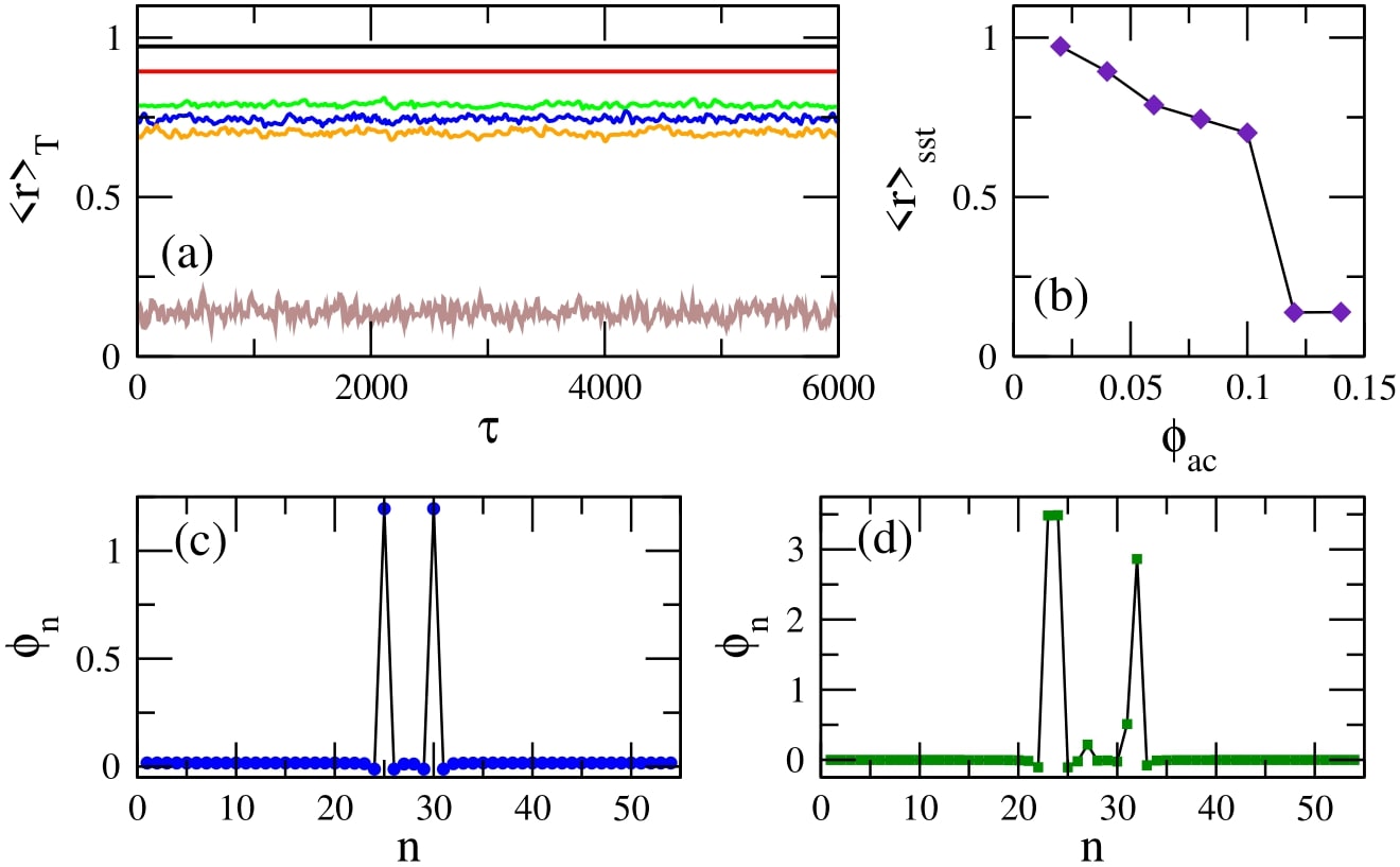
Figure 7: (a) The magnitude of the synchronization parameter averaged over the driving period, ${\langle r\rangle}_{T}$, as a function of time $\tau$ for $\beta_{L}=0.86$, $\gamma=0.01$, $\lambda=-0.02$, $\Omega=1.01$, $N=54$, $\phi_{dc}=0$, and $\phi_{ac}=0.02$ (black), $\phi_{ac}=0.04$ (red), $\phi_{ac}=0.06$ (green), $\phi_{ac}=0.08$ (blue), $\phi_{ac}=0.10$ (orange), $\phi_{ac}=0.12$ (brown). (b) The magnitude of the synchronization parameter averaged over the steady-state integration time $\tau_{sst}$, ${\langle r\rangle}_{sst}$, as a function of the ac flux amplitude $\phi_{ac}$. The other parameters are as in (a). (c) The flux profile $\phi_{n}$ for $\phi_{ac}=0.02$ and the other parameters as in (a). (d) The flux profile $\phi_{n}$ for $\phi_{ac}=0.04$ and the other parameters as in (a).

Another set of initial conditions which gives rise to chimera states is of the form Hizanidis et al. (2016a)

$$\phi_{n}(\tau=0)=\frac{1}{2}\cos\left(\frac{2j\pi n}{N}\right),\qquad\dot{\phi}_{n}(\tau=0)=0,$$ (38)

where $n=1,...,N$. The initial conditions in Eq. (38) allow for generating multiclustered chimera states, in which the number of clusters depends on $j$. In Figs. 8(a) and (b), maps of ${\langle\dot{\phi}_{n}\rangle}_{T}$ on the $n-\tau$ plane for $j=1$ and $j=2$, respectively, are shown. In Fig. 8(a), three large clusters can be distinguished; in the two of them, the SQUID oscillators are synchronized, while in the third one, in between the two sychronized clusters, the SQUID oscillators are desynchronized. The flux profile $\phi_{n}$ of that state at the end of the steady-state integration time $\tau_{sst}=6000$, is shown in Fig. 8(c) as blue circles (the black curve is a guide to the eye) along with the initial condition (red curve). It can be seen that two more desynchronized clusters at the ends of the metamaterial, which are rather small (they consist of only a few SQUIDs each), are visible. Obviously, the synchronized clusters correspond to the spatial interval indicated by the almost horizontal segments in the $\phi_{n}$ profile. The corresponding ${\langle\dot{\phi}_{n}\rangle}_{T}$ map and flux profile $\phi_{n}$ for $j=2$ is shown in Figs. 8(b) and (d), respectively. In this case, a number of six (6) synchronized clusters and seven (7) desynchronized clusters are visible in both Figs. 8(b) and (d). In Figs. 8(d), the red curve is the initial condition from Eq. (38) with $j=2$. Chimera states with even more “heads” can be generated from the initial condition Eq. (38) for $j>2$ in larger systems (here $N=54$).

Similar chimera states can be generated with local (nearest-neighbor) coupling between the SQUIDs of the metamaterial. For that purpose, Eq. (III.1) is integrated in time using a fourth order Runge-Kutta algorithm with free-end boundary conditions and the initial conditions of Eq. (33). As above, in order to eliminate transients and reach a steady-state, Eq. (III.1) is integrated for $10^{7}~{}T$ time units and the results are discarded. Then, (III.1) is integrated for $\tau_{sst}=10^{3}~{}T$ more time units (steady-state integration time), and ${\langle\dot{\phi}_{n}\rangle}_{T}$ is mapped on the $n-\tau$ plane (Fig. 9). The emerged states are very similar to those shown in Fig. 6, which is the case of non-local coupling between the SQUIDs. In particular, the states shown in Fig. 9(a), (b), and (c), have been generated for exactly the same parameters and initial-boundary conditions as those in Fig. 6(c), (e), and (f), respectively, i.e, for $\phi_{ac}=0.06$, $0.1$, and $0.12$. Note that the state of the SQUID metamaterial for $\phi_{ac}=0.12$ is completely desynchronized both in Fig. 6(f) and 9(c). One may also compare the plots of the corresponding ${\langle r\rangle}_{T}$ as a function of $\tau$, which are shown in Fig. 9(d) for the local coupling case. The averages of $r$ over the steady-state integration time $\tau_{sst}$ for $\phi_{ac}=0.06$, $0.1$, $0.12$ are, respectively, ${\langle r\rangle}_{sst}=0.757$, $0.656$, $0.136$ for the nonlocal coupling case and ${\langle r\rangle}_{sst}=0.743$, $0.656$, $0.146$ for the local coupling case. The probability distribution function of the values of ${\langle r\rangle}_{T}$, $pdf({\langle r\rangle}_{T})$, for the three states in Figs. 9(a)-(c) are shown in Figs. 9(e)-(g), respectively. As it was mentioned above, the FWHM of such a distribution is a measure of the metastability of the corresponding chimera state. The FWHM for the distributions in Fig. 9(e) and (f), calculated for the chimera states shown in Fig. 9(a) and (b), are respectively $0.003$ and $0.0215$. Thus, it can be concluded that the chimera state of Fig. 9(b) is more metastable than that in Fig. 9(a). The distribution in Fig. 9(g) has a FWHM much larger than the ones of the distributions in Figs. 9(e) and (f) as expected, since it has been calculated for the completely desynchronized state of Fig. 9(c). Note that $10^{6}$ values of ${\langle r\rangle}_{T}$ have been used to obtain each of the three distributions. Also, these distributions are normalized such that their area sums to unity.

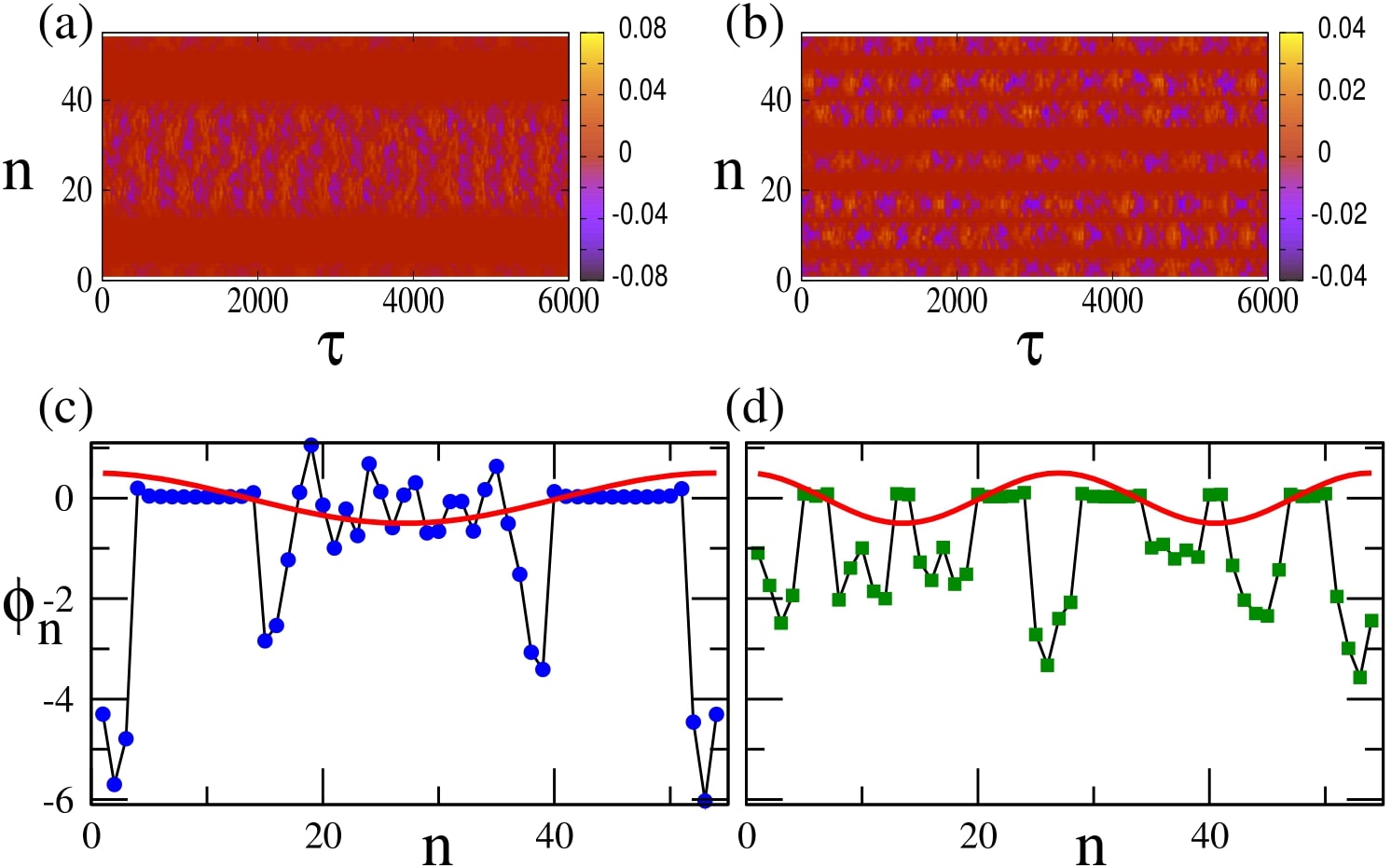
Figure 8: (a) Map of ${\langle\dot{\phi}_{n}\rangle}_{T}$ on the $n-\tau$ plane for $\beta_{L}=0.86$, $\gamma=0.01$, $\lambda=-0.02$, $\Omega=1.01$, $N=54$, $\phi_{dc}=0$, $\phi_{ac}=0.1$, and initial conditions given by Eq. (38) with $j=1$. (b) Same as in (a) with initial conditions given by Eq. (38) with $j=2$. (c) Flux profile $\phi_{n}$ at the end of the steady-state integration time (blue circles, the black line is a guided to the eye), obtained with the initial conditions Eq. (38) with $j=1$ (red curve). (d) Flux profile $\phi_{n}$ at the end of the steady-state integration time (blue circles, the black line is a guided to the eye), obtained with the initial conditions Eq. (38) with $j=2$ (red curve).

The chimera states do not result from destabilization of the synchronized state of the SQUID metamaterial; instead, they coexist with the latter, which can be reached simply by integrating the relevant flux dynamics equations with zero initial conditions, i. e., with $\phi_{n}(\tau=0)=0$ and $\dot{\phi}_{n}(\tau=0)=0$ for any $n$. In order to reach a chimera state, on the other hand, appropriately chosen initial conditions such as those in Eq. (33) or Eq. (38) have to be used. However, one cannot expect that the synchronized state is stable over the whole external parameter space, i. e., the ac flux amplitude $\phi_{ac}$, the frequency of the ac flux field $\Omega$, and the dc flux bias $\phi_{dc}$. In order to explore the stability of the synchronized state of the SQUID metamaterial, the magnitude of the synchronization parameter averaged over the steady-state integration time, ${\langle r\rangle}_{sst}$, is calculated and then mapped on the $\phi_{dc}-\phi_{ac}$ parameter plane. For each pair of $\phi_{ac}$ and $\phi_{dc}$ values, the SQUID metamaterial is initialized with zeros (it is at “rest”). Once again, the frequency $\Omega$ is chosen to be very close to the geometrical resonance $\Omega_{LC}$ ($\Omega\simeq 1$). In Fig. 10, maps of ${\langle r\rangle}_{sst}$ on the $\phi_{dc}-\phi_{ac}$ plane are shown for four driving frequencies $\Omega$ around unity. These maps are a kind of “synchronization phase diagrams”, in which ${\langle r\rangle}_{sst}=1$ indicates a synchronized state while ${\langle r\rangle}_{sst}<1$ indicates a partially or completely desynchronized state. In all subfigures, but perhaps most clearly seen in Fig. 10(c) (for $\Omega=1.01$) there are abrupt transitions between completely synchronized (red areas) and completely desynchronized (light blue areas) states. It can be verified by inspection of the flux profiles (not shown) that these synchronization-desynchronization transitions do not go through a stage in which chimera states are generated; instead, the destabilization of a synchronized state results either in a completely desynchronized state (light blue areas) or a clustered state (green areas). Thus, it seems that chimera states cannot be generated when the SQUID metamaterial is initially at “rest”, i. e., with zero initial conditions. As we shall see in the next Section (Section 5), this is not true for a position-dependent external flux $\phi_{ext}=\phi_{ext}(n)$.

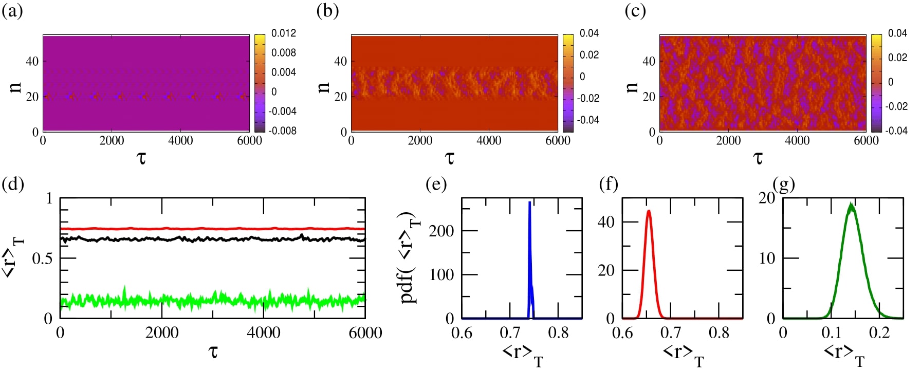
Figure 9: (a) Map of ${\langle\dot{\phi}_{n}\rangle}_{T}$ on the $n-\tau$ plane for $\beta_{L}=0.86$, $\gamma=0.01$, $\lambda=-0.02$, $\Omega=1.01$, $N=54$, $\phi_{dc}=0$, $\phi_{ac}=0.06$, and initial conditions given by Eq. (33). (b) Same as in (a) but with $\phi_{ac}=0.10$. (c) Same as in (a) and (b) but with $\phi_{ac}=0.12$. (d) The magnitude of the synchronization parameter averaged over the driving period, ${\langle r\rangle}_{T}$, as a function of time $\tau$ for $\phi_{ac}=0.06$ (red), $\phi_{ac}=0.1$ (black), and $\phi_{ac}=0.12$ (green). The other parameters are as in (a). (e) The distribution of $10^{6}$ values of ${\langle r\rangle}_{T}$, $pdf({\langle r\rangle}_{T})$, for the chimera state shown in (a). (f) Same as in (e) for the chimera state shown in (b). (g) Same as in (e) and (f) for the completely desynchronized state shown in (c).

V Chimera generation by dc flux gradients

V.1 Modified flux dynamics equations

In obtaining the results of Fig. 10, a spatially homogeneous dc flux $\phi_{dc}$ over the whole SQUID metamaterial is considered. Although, all the chimera states presented here are generated at $\phi_{dc}=0$, such states can be also generated in the presence of a spatially constant, non-zero $\phi_{dc}$, by using appropriate initial conditions (not shown here). In this Section, the generation of chimera states in SQUID metamaterials driven by an ac flux and biased by a dc flux gradient is demonstrated, for the SQUID metamaterial being initially at “rest”. The application of a dc flux gradient along the SQUID metamaterial is experimentally feasible with the set-up of Ref. Zhang et al. (2015). Consider the SQUID metamaterial model in Section $3.1$ in the case of local coupling (for simplicity), in which the dc flux is assumed to be position-dependent, i. e., $\phi_{dc}=\phi_{n}^{dc}$. Then, Eqs. (III.1) can be easily modified to become

$$\ddot{\phi}_{n}+\gamma\dot{\phi}_{n}+\phi_{n}+\beta\,\sin(2\pi\phi_{n})=\phi_{n}^{eff}(\tau)$$

$$+\lambda(\phi_{n-1}+\phi_{n+1}),$$ (39)

where

$$\phi_{n}^{eff}=\phi_{n}^{ext}-\lambda(\phi_{n-1}^{ext}+\phi_{n+1}^{ext}),$$ (40)

with

$$\phi_{n}^{ext}=\phi_{n}^{dc}+\phi_{ac}\cos(\Omega\tau).$$ (41)

In the following, the dc flux function $\phi_{n}^{dc}$ is assumed to be of the form

$$\phi_{n}^{dc}=\frac{n-1}{N-1}\phi_{max}^{dc},~{}~{}~{}~{}~{}~{}n=1,...,N,$$ (42)

so that the dc flux bias increases linearly from zero (for the SQUID at $n=1$) to $\phi_{max}^{dc}$ (for the SQUID at the $n=N$).

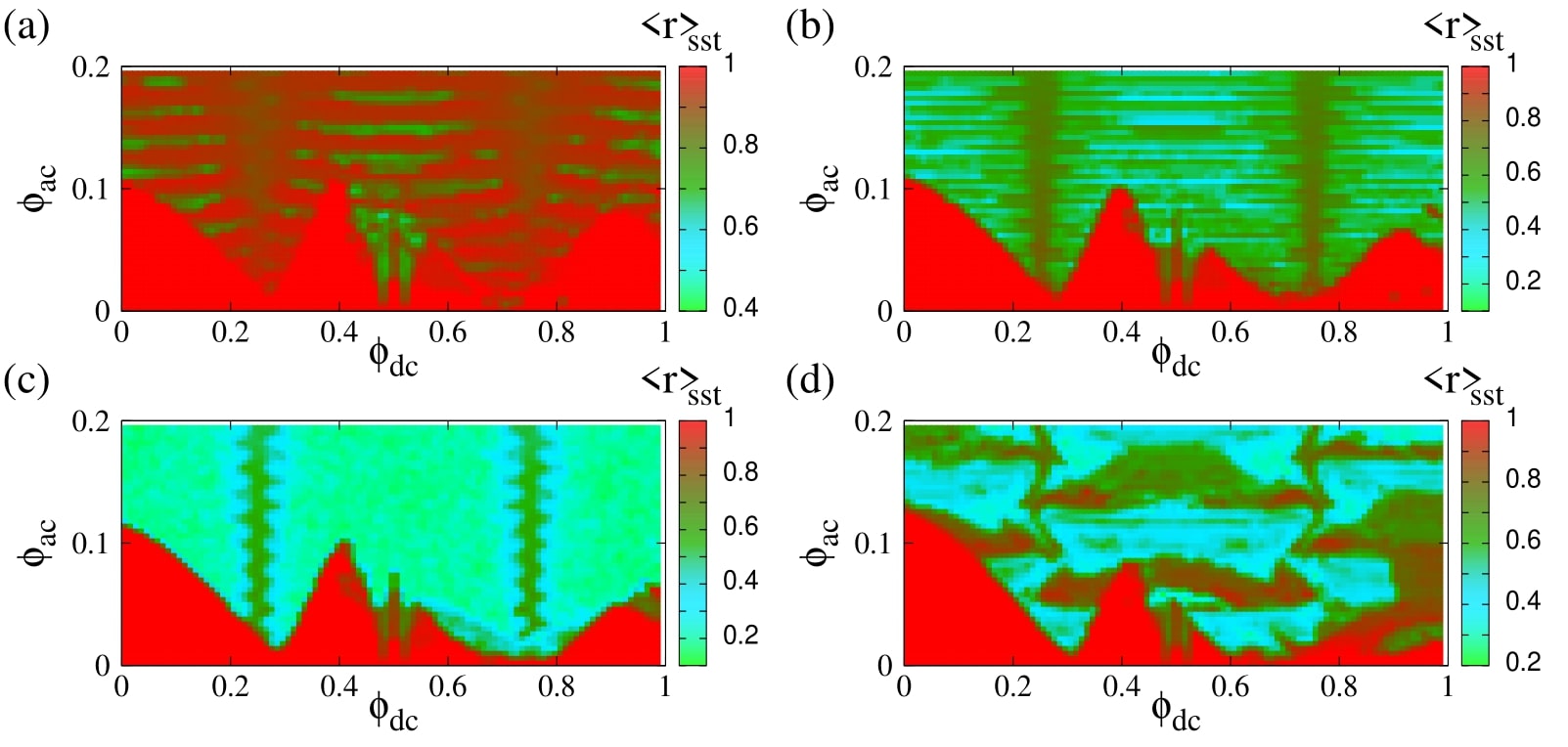
Figure 10: Map of the magnitude of the synchronization parameter averaged over the steady-state integration time, ${\langle r\rangle}_{sst}$, on the dc flux bias - ac flux amplitude ($\phi_{dc}-\phi_{ac}$) parameter plane, for $\beta_{L}=0.86$, $\gamma=0.01$, $\lambda=-0.02$, $N=54$, and (a) $\Omega=1.03$, (b) $\Omega=1.02$, (c) $\Omega=1.01$, (d) $\Omega=0.982$.

V.2 Generation and control of chimera states

Equations (V.1) are integrated numerically in time with free-end boundary conditions (Eqs. (V.1)) using a fourth-order Runge-Kutta algorithm with time-step $h=0.02$. The SQUID metamaterial is initially at “rest”, i. e.,

$$\phi_{n}(\tau=0)=0,\qquad\dot{\phi}_{n}(\tau=0)=0,~{}~{}~{}~{}n=1,...,N.$$ (43)

This system is integrated for $10^{5}~{}T$ time units to eliminate the transients and then for more $\tau_{sst}=10^{5}~{}T$ time units during which the temporal averages ${\langle r\rangle}_{sst}$ and ${\langle r\rangle}_{T}(\tau)$ are calculated. Note that the transients die-out faster in this case since the SQUID metamaterial is initialized with zeros.

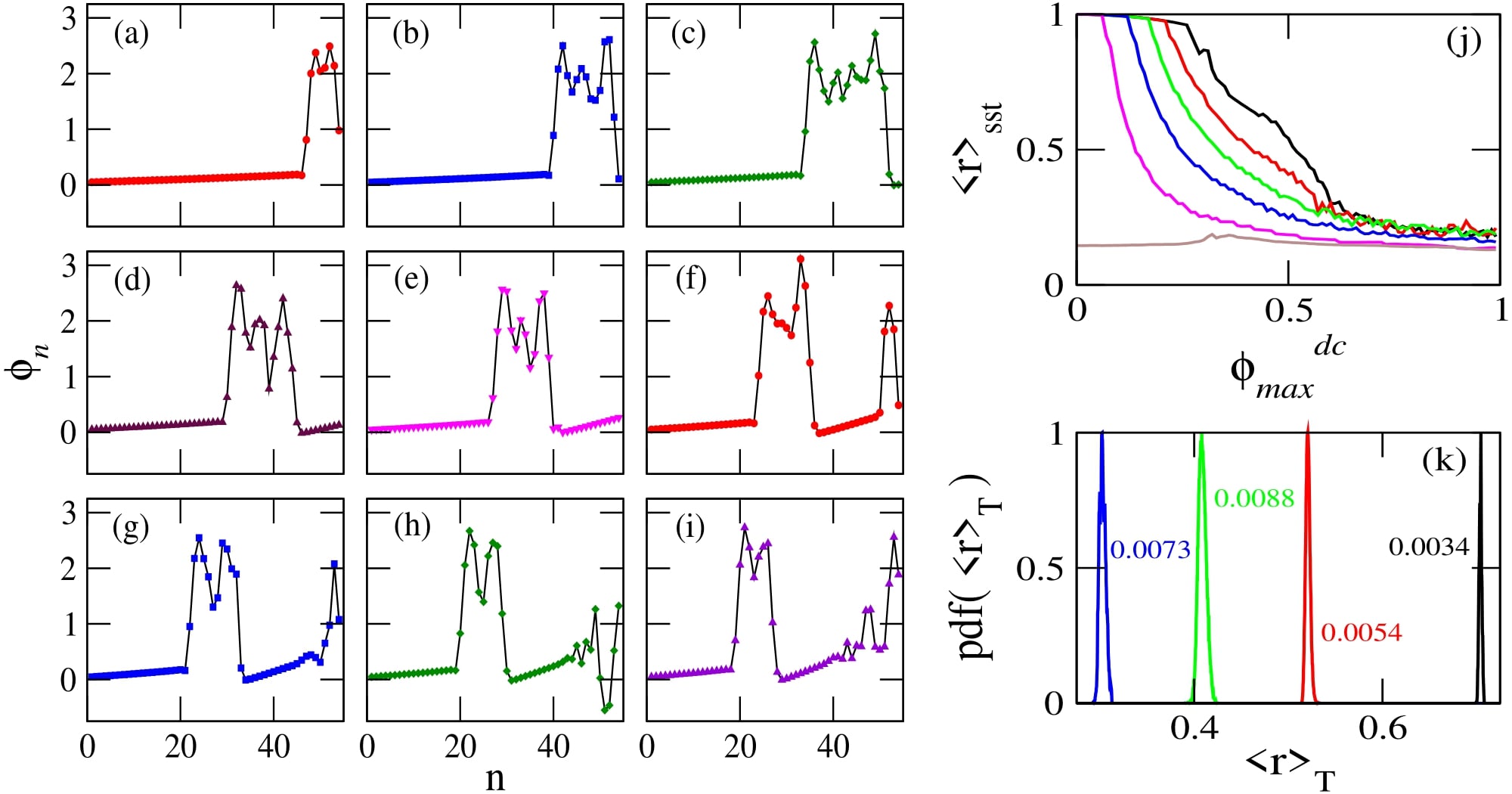
Figure 11: Flux profiles $\phi_{n}$ as a function of $n$ for $\beta_{L}=0.86$, $\gamma=0.01$, $\lambda=-0.02$, $N=54$, $\phi_{ac}=0.04$, $\Omega=1.01$, and (a) $\phi_{max}^{dc}=0.25$; (b) $0.30$; (c) $0.35$; (d) $0.40$; (e) $0.45$; (f) $0.50$; (g) $0.55$; (h) $0.60$; (i) $0.65$. (j) The magnitude of the synchronization parameter averaged over the steady-state integration time ${\langle r\rangle}_{sst}$ as a function of $\phi_{max}^{dc}$ for the parameters of (a)-(i) but with $\phi_{ac}=0.02$ (black), $0.04$ (red), $0.06$ (green), $0.08$ (blue), $0.10$ (magenta), $0.12$ (brown). (k) Distributions of the values of ${\langle r\rangle}_{T}$ for $\phi_{ac}=0.04$, and $\phi_{max}^{dc}=0.30$ (black), $0.40$ (red), $0.50$ (green), $0.60$ (blue). The other parameters as in (a)-(i). The numbers next to the distributions are the corresponding full-width half-maximums.

Typical flux profiles $\phi_{n}$, plotted at the end of the steady-state integration time are shown in Figs. 11(a)-(i). The varying parameter in this case is $\phi_{max}^{dc}$, which actually determines the gradient of the dc flux. The state of the SQUID metamaterial remains almost homogeneous in space for $\phi_{max}^{dc}$ increasing from zero to $\phi_{max}^{dc}=0.22$. At that critical value of $\phi_{max}^{dc}$, the spatially homogeneous (almost synchronized) state breaks down, for several SQUIDs close to $n=N$ become desynchronized with the rest (because the dc flux is higher at this end). The number of desynchronized SQUIDs for $\phi_{max}^{dc}=0.25$ is about $6-7$ (Fig. 11(a)). For further increasing $\phi_{max}^{dc}$, more and more SQUIDs become desynchronized, until they form a well-defined desynchronized cluster (Fig. 11(b) for $\phi_{max}^{dc}=0.30$). As $\phi_{max}^{dc}$ continues to increase, the desynchronized cluster clearly shifts to the left, i. e., towards $n=1$ (Fig. 11(c)-(e)). Further increase of $\phi_{max}^{dc}$ generates a second desynchronized cluster around $n=N$ for $\phi_{max}^{dc}=0.50$ (Fig. 11(f)), which persists for values of $\phi_{max}^{dc}$ at least up to $0.65$. With the formation of the second desynchronized cluster, the first one clearly becomes smaller and smaller with increasing $\phi_{max}^{dc}$ (see Figs. 11(f)-(i)). Above, the expression “almost homogeneous” was used instead of simply “homogeneous”, because complete homogeneity is not possible due to the dc flux gradient. However, for $\phi_{max}^{dc}<0.22$, the degree of homogeneity (synchronization) is more than $99\%$, i. e., the values of the synchronization parameter ${\langle r\rangle}_{sst}$ are higher than $0.99$ (${\langle r\rangle}_{sst}>0.99$). The dependence of ${\langle r\rangle}_{sst}$ on $\phi_{max}^{dc}$ for several values of the ac flux amplitude $\phi_{ac}$ is shown in Fig. 11(j). The SQUID metamaterial remains in an almost synchronized state (with ${\langle r\rangle}_{sst}>0.96$ below a critical value of $\phi_{max}^{dc}$, which depends on the ac flux amplitude $\phi_{ac}$. That critical value of $\phi_{max}^{dc}$ is lower for higher $\phi_{ac}$. For values of $\phi_{max}^{dc}$ higher than the critical one, ${\langle r\rangle}_{sst}$ gradually decreases until it saturates at ${\langle r\rangle}_{sst}\simeq 0.12$. For $\phi_{ac}=0.12$, the SQUID metamaterial is in a completely desynchronized state for any value of $\phi_{max}^{dc}$ (brown curve). The distributions of the values of ${\langle r\rangle}_{T}$, obtained during the steady-state integration time, are shown in Fig. 11(k) for $\phi_{max}^{dc}=0.30$ (black), $0.40$ (red), $0.50$ (green), and $0.60$ (blue). As expected, the maximum of the distributions shifts to lower ${\langle r\rangle}_{T}$ with increasing $\phi_{max}^{dc}$. These distributions have been divided by their maximum value for easiness of presentation, and the number next to each distribution is its full-width half-maximum (FWHM).

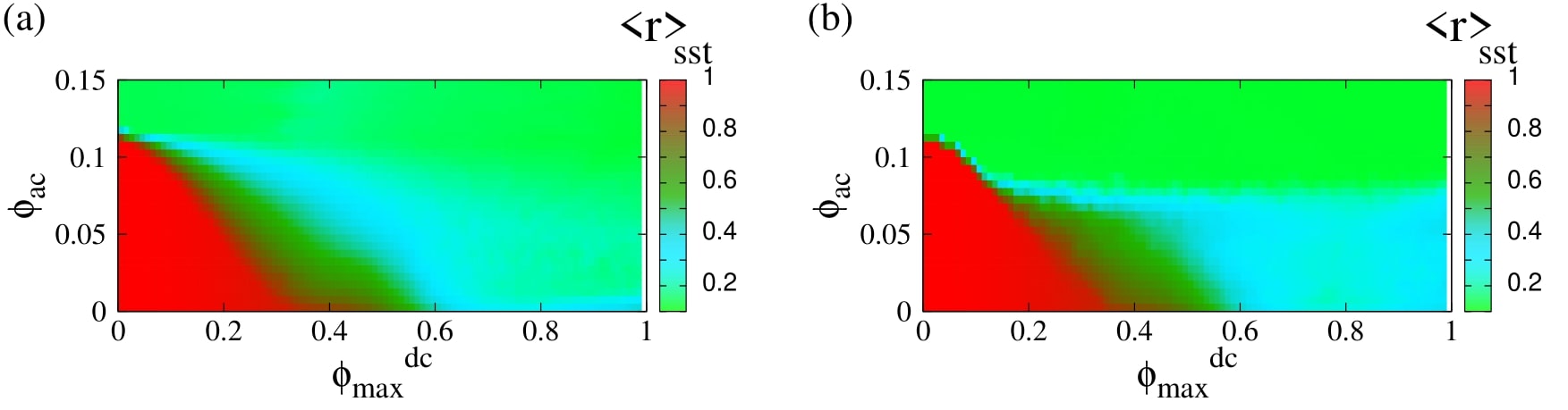
Figure 12: The magnitude of the synchronization parameter averaged over the steady-state integration time ${\langle r\rangle}_{sst}$ mapped as a function of the ac flux amplitude and the maximum dc flux bias ($\phi_{ac}-\phi_{max}^{dc}$ plane), for $\beta_{L}=0.86$, $\gamma=0.01$, $N=54$, $\Omega=1.01$, and (a) $\lambda=-0.02$, (b) $\lambda=-0.06$.

Two typical “synchronization phase diagrams”, in which ${\langle r\rangle}_{sst}$ is mapped on the $\phi_{ac}-\phi_{max}^{dc}$ parameter plane, are shown in Figs. 12(a) and (b) for $\lambda=-0.02$ and $\lambda=-0.06$, respectively. The frequency of the driving ac field has been chosen once again to be very close to the geometrical resonance of a single SQUID oscillator, i. e., at $\Omega=1.01$. For each point on the $\phi_{ac}-\phi_{max}^{dc}$ plane, Eqs. (V.1) are integrated in time with a standard fourth order Runge-Kutta algorithm using the initial conditions of Eq. (43), with a time-step $h=0.02$. First, Eqs. (V.1) are integrated for $10^{5}~{}T$ time-units to eliminate transients, and then they are integrated for $\tau_{sst}=10^{5}~{}T$ more time-units during which ${\langle r\rangle}_{sst}$ is calculated. A comparison between Fig. 12(a) and (b) reveals that the increase of the coupling strength between nearest-neighboring SQUIDs from $\lambda=-0.02$ to $\lambda=-0.06$ results in relatively moderate, quantitative differences only. In both Figs. 12(a) and (b), for values of $\phi_{ac}$ and $\phi_{max}^{dc}$ in the red areas, the state of the SQUID metamaterial is synchronized. For values of $\phi_{ac}$ and $\phi_{max}^{dc}$ in the dark-green, light-green and light-blue areas, the state of the SQUID metamaterial is either completely desynchronized, or a chimera state with one or more desynchronized clusters. In order to obtain more information about these states, additional measures should be used, such as the incoherence index $S$ and the chimera index $\eta$ Gopal et al. (2014, 2018). These are defined as follows: First, define

$$v_{n}(\tau)\equiv{\langle\dot{\phi}_{n}\rangle}_{T}(\tau),$$ (44)

where the angular brackets denote averaging over $T$, and

$$\bar{v}_{n}(\tau)\equiv\frac{1}{n_{0}+1}\sum_{n=-n_{0}/2}^{+n_{0}/2}v_{n}(\tau),$$ (45)

the local spatial average of $v_{n}(\tau)$ in a region of length $n_{0}+1$ around the site $n$ at time $\tau$ ($n_{0}<N$ is an integer). Then, the local standard deviation of $v_{n}(\tau)$ is defined as

$$\sigma_{n}(\tau)\equiv\left<\sqrt{\frac{1}{n_{0}+1}\sum_{n=-n_{0}/2}^{+n_{0}/2}\left(v_{n}-\bar{v}_{n}\right)^{2}}\right>_{sst},$$ (46)

where the large angular brackets denote averaging over the steady-state integration time. The index of incoherence is then defined as

$$S=1-\frac{1}{N}\sum_{n=1}^{N}s_{n},$$ (47)

where $s_{n}=\Theta(\delta-\sigma_{n})$ with $\Theta$ being the Theta function. The index $S$ takes its values in $[0,1]$, with $0$ and $1$ corresponding to synchronized and desynchronized states, respectively, while all other values between them indicate the existence of a chimera or multi-chimera state. Finally, the chimera index is defined as

$$\eta=\sum_{n=1}^{N}|s_{n}-s_{n+1}|/2,$$ (48)

and takes positive integer values. The chimera index $\eta$ gives the number of desynchronized clusters of a (multi-)chimera state, except in the case of a completely desynchronized state where it gives zero. In Fig. 13, the incoherence index $S$ and the chimera index $\eta$ are mapped on the $\phi_{ac}-\phi_{max}^{dc}$ plane for the same parameters as in Fig. 12(a).

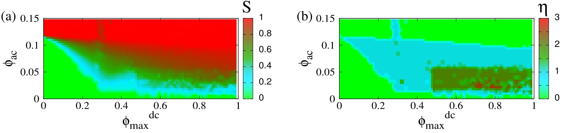
Figure 13: The index of incoherence $S$ and the chimera index $\eta$ are mapped on the $\phi_{ac}-\phi_{max}^{dc}$ plane, for the same parameters as in Fig. 12(a) and $n_{0}=4$, $\delta=10^{-4}$.

Figs. 13(a) and (b) provide more information about the state of the SQUID metamaterial at a particular point on the $\phi_{ac}-\phi_{max}^{dc}$ plane. In Fig. 13(a), for values of $\phi_{ac}$ and $\phi_{max}^{dc}$ in the light-green area ($S=0$) the SQUID metamaterial is in a synchronized state (see the corresponding area in Fig. 13(b) in which $\eta=0$). For values of $\phi_{ac}$ and $\phi_{max}^{dc}$ in the red area ($S=1$), the SQUID metamaterial is completely desynchronized (the corresponding area in Fig. 13(b) has $\eta=0$ due to technical reasons). For values of $\phi_{ac}$ and $\phi_{max}^{dc}$ in one of the other areas, the SQUID metamaterial is in a chimera state with one, two, or three desynchronized clusters, as it can be inferred from Fig. 13(b).

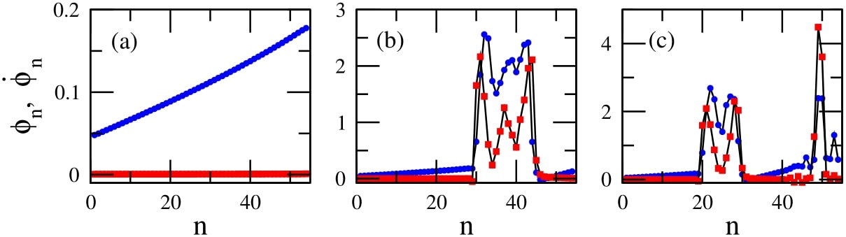
Figure 14: Flux and voltage profiles $\phi_{n}$ (blue) and $v_{n}=\dot{\phi}_{n}$ (red), respectively, as a function of $n$ for $\beta_{L}=0.86$, $\gamma=0.01$, $\Omega=1.01$, $\phi_{ac}=0.04$, and (a) $\phi_{max}^{dc}=0.2$, (b) $\phi_{max}^{dc}=0.4$, (c) $\phi_{max}^{dc}=0.6$.

Using the combined information from Figs. 12 and 13, the form of the steady-state of a SQUID metamaterial can be predicted for any physically relevant value of $\phi_{ac}$ and $\phi_{max}^{dc}$. In Fig. 14, three flux profiles $\phi_{n}$ are shown as a function of $n$, along with the corresponding profiles of their time-derivatives, $\dot{\phi}_{n}$. The profiles in Figs. 14(a), (b), and (c), are obtained for $\phi_{ac}=0.04$ and $\phi_{max}^{dc}=0.2$, $0.4$, and $0.6$, respectively, which are located in the light-green, light-blue, and dark-green area of Fig. 14(b). As it is expected, the state in Fig. 14(a) is an almost synchronized one, in Fig. 14(b) is a chimera state with one desynchronized cluster, while in Fig. 14(c) is a chimera state with two desynchronized clusters. At this point, the use of the expression “almost synchronized” should be explained. In the presence of a dc flux gradient, it is impossible for a SQUID metamaterial to reach a completely synchronized state. This is because each SQUID is subject to a different dc flux, which modifies accordingly its resonance (eigen-)frequency. As a result, the flux oscillation amplitudes of the SQUIDs, whose oscillations are driven by the ac flux field of amplitude $\phi_{ac}$ and frequency $\Omega$, are slightly different. On the other hand, the maximum of the flux oscillations for all the SQUIDs is attained at the same time. Indeed, as can be observed in Fig. 14(a). the flux profile $\phi_{n}$ is not horizontal, as it should be in the case of complete synchronization. Instead, that profile increases almost linearly from $n=1$ to $n=N$ (that increase is related to the dc flux gradient). However, the voltage profile $\dot{\phi}_{n}$ is zero for any $n$, indicating that all the SQUID oscillators are in phase. Since, in such a state of the SQUID metamaterial there is phase synchronization but no amplitude synchronization, the synchronization is not complete. However, the value of ${\langle r\rangle}_{sst}$ in such a state is in the worst case higher than $0.96$ for moderately high values of $\phi_{ac}=0.02-0.10$ (Fig. 11(j)), which is a very high degree of global synchronization. Furthermore, the synchronized clusters in the chimera state profiles in Figs. 14(b) and (c), whose length coincides with that of the horizontal segments of the $\dot{\phi_{n}}$ profiles, also exhibit a very high degree of global synchronization (${\langle r\rangle}_{sst}>0.96$).

VI Discussion and Conclusions

The emergence of chimera and multi-chimera states in a 1D SQUID metamaterial driven by an ac flux field is demonstrated numerically, using a well-established model that relies on equivalent electrical circuits. Chimera states may emerge both with local coupling between SQUID (nearest-neighbor coupling) and nonlocal coupling between SQUIDs which falls-off as the inverse cube of their center-to-center distance. A large variety of initial conditions can generate chimera states which persist for very long times. In the previous Sections, the expression “steady-state integration time” is used repeatedly; however, in some cases this may not be very accurate, since chimera states are generally metastable and sudden changes may occur at any instant of time-integration which results in sudden jumps the synchronization parameter ${\langle r\rangle}_{T}$ Lazarides et al. (2015). For the chimera states presented here, however, no such sudden changes have been observed. Along with the ac flux field, a dc flux bias, the same at any SQUID, can be also applied to the 1D SQUID metamaterial. Chimera states can be generated in that case as well, although not shown here.

The emergence of those counter-intuitive states, their form and their global degree of synchronization depends crucially on the initial conditions. If the SQUID metamaterial is initialized with zeros, the generation of chimera states does not seem to be possible for spatially constant dc flux bias $\phi_{dc}$. In that case, synchronization-desynchronization and reverse synchronization-desynchronization transitions may occur by varying the ac flux amplitude $\phi_{ac}$ or the dc flux bias $\phi_{dc}$. In the former transition, a completely synchronized state suddenly becomes a completely desynchronized one. The replacement of the spatially constant dc flux bias by a position-dependent one, $\phi_{n}^{dc}$, makes possible the generation of chimera states from zero initial conditions. Here, a dc flux gradient is applied to the SQUID metamaterial, which provides the possibility to control the chimera state. Indeed, it is demonstrated that the position of the desynchronized cluster(s) and the global degree of synchronization can be controlled to some extent by varying the dc flux gradient. Moreover, in the presence of a dc flux gradient, the ac flux amplitude controls the size of the desynchronized cluster.

Here, the driving frequency is always chosen to be very close to the geometrical frequency of the individual SQUIDs. In the case of relatively strong nonlinearity, considered here, the resonance frequency of individual SQUIDs is shifted to practically around the geometrical frequency. That is, for relatively strong nonlinearity, the driving frequency was chosen so that the SQUIDs are at resonance. For a single SQUID driven close to its resonance, the relatively strong nonlinearity makes it highly multistable; then, several stable and unstable single SQUID states may coexist (see the snake-like curves presented in Section 2). This dynamic multistability effect is of major importance for the emergence of chimera states in SQUID metamaterials, as it is explained below.

The dynamic complexity of $N$ SQUIDs which are coupled together increases with increasing $N$; this effect has been described in the past for certain arrays of coupled nonlinear oscillators as attractor crowding Wiesenfeld and Hadley (1989); Tsang and Wiesenfeld (1990). This complexity is visible already for two coupled SQUIDs, where the number of stable states close to the geometrical resonance increases more than two times compared to that of a single SQUID Hizanidis et al. (2016a); some of these states can even be chaotic. Interestingly, the existence of homoclinic chaos in a pair of coupled SQUIDs has been proved by analytical means Agaoglou et al. (2015, 2017). It has been argued that the number of stable limit cycles (i. e., periodic solutions) in such systems scales with the number of oscillators $N$ as $(N-1)!$. As a result, their basins of attraction crowd more and more tightly in phase space with increasing $N$. The multistability of individual SQUIDs around the resonance frequency enhances the attractor crowding effect in SQUID metamaterial. Apart from the large number of periodic solutions (limit cycles), a number of coexisting chaotic solutions may also appear as in the two-SQUID system. All these states are available for each SQUID to occupy. Then, with appropriate initialization of the SQUID metamaterial, or by applying a dc flux gradient to it, a number of SQUIDs that belong to the same cluster may occupy a chaotic state. The flux oscillations of these SQUIDs then generally differ in both their amplitude and phase, resulting for that cluster to be desynchronized. Alternatingly, a number of SQUIDs that belong to the same cluster may find themselves in a region of phase-space with a high density of periodic solutions. Then, the flux in these SQUID oscillators may jump irregularly from one periodic state to another resulting in effectively random dynamics and in effect for that cluster to be desynchronized. At the same time, the other cluster(s) of SQUIDs can remain synchronized and, as a result, a chimera state emerges.

Conflict of Interest Statement

The authors declare that the research was conducted in the absence of any commercial or financial relationships that could be construed as a potential conflict of interest.

Author Contributions

NL conceived the structure of the manuscript, JH and NL performed the simulations, and all authors listed performed data analysis and have made intellectual contribution to the work, and approved it for publication.

References

- Smith et al. (2004) Smith DR, Pendry JB, Wiltshire. Metamaterials and negative refractive index. Science Vol. 305 no. 5685 (2004) 788–792.
- Linden et al. (2006) Linden S, Enkrich C, Dolling G, Klein MW, Zhou J, Koschny T, et al. Photonic metamaterials: magnetism at optical frequencies. IEEE J. Selec. Top. Quant. Electron. 12 (2006) 1097–1105.
- Padilla et al. (2006) Padilla WJ, Basov DN, Smith DR. Negative refractive index metamaterials. Materials Today 9 (7-8) (2006) 28–35.
- Shalaev (2007) Shalaev VM. Optical negative-index metamaterials. Nature Photon. 1 (2007) 41–48.
- Litchinitser and Shalaev (2008) Litchinitser NM, Shalaev VM. Photonic metamaterials. Laser Phys. Lett. 5 (2008) 411–420.
- Soukoulis and Wegener (2011) Soukoulis CM, Wegener M. Past achievements and future challenges in the development of three-dimensional photonic metamaterials. Nature Photon. 5 (2011) 523–530.
- Liu and Zhang (2011) Liu Y, Zhang X. Metamaterials: a new frontier of science and technology. Chem. Soc. Rev. 40 (2011) 2494–2507.
- Simovski et al. (2012) Simovski CR, Belov PA, Atrashchenko AV, Kivshar YS. Wire metamaterials: Physics and applications. Adv. Mater. 24 (2012) 4229–4248.
- Engheta and Ziokowski (2006) Engheta N, Ziokowski RW. Metamaterials: Physics and engineering explorations (Wiley-IEEE Press) (2006).
- Pendry (2007) Pendry JB. Fundamentals and applications of negative refraction in metamaterials (Princeton University Press) (2007).
- Ramakrishna and Grzegorczyk (2009) Ramakrishna SA, Grzegorczyk T. Physics and applications of negative refractive index materials (SPIE and CRC Press) (2009).
- Cui et al. (2010) Cui TJ, Smith DR, Liu R. Metamaterials theory, design and applications (Springer: Springer) (2010).
- Cai and Shalaev (2010) Cai W, Shalaev V. Optical metamaterials, fundamentals and applications (Heidelberg: Springer) (2010).
- Solymar and Shamonina (2009) Solymar L, Shamonina E. Waves in metamaterials (New York: Oxford University Press) (2009).
- Noginov and Podolskiy (2012) Noginov MA, Podolskiy VA. Tutorials in metamaterials (Taylor Francis) (2012).
- Tong (2018) Tong XC. Functional Metamaterials and Metadevices, Springer Series in Materials Science Vol.262 (Springer International Publishing AG 2018) (2018).
- Anlage (2011) Anlage SM. The physics and applications of superconducting metamaterials. J. Opt. 13 (2011) 024001–10.
- Jung et al. (2014a) Jung P, Ustinov AV, Anlage SM. Progress in superconducting metamaterials. Supercond. Sci. Technol. 27 (2014a) 073001 (13pp).
- Jin et al. (2010) Jin B, Zhang C, Engelbrecht S, Pimenov A, Wu J, Xu Q, et al. Low loss and magnetic field-tunable superconducting terahertz metamaterials. Opt. Express 18 (2010) 17504–17509.
- Zhang et al. (2012) Zhang CH, Wu JB, Jin BB, Ji ZM, Kang L, Xu WW, et al. Low-loss terahertz metamaterial from superconducting niobium nitride films. Opt. Express 20 (1) (2012) 42–47.
- Gu et al. (2010) Gu J, Singh R, Tian Z, Cao W, Xing Q, He MX, et al. Terahertz superconductor metamaterial. Appl. Phys. Lett. 97 (2010) 071102 (3pp).
- Zhang et al. (2014) Zhang X, Gu J, Han J, Zhang W. Tailoring electromagnetic responses in terahertz superconducting metamaterials. Frontiers of Optoelectronics 8(1) (2014) 44–56.
- Du et al. (2006) Du C, Chen H, Li S. Quantum left-handed metamaterial from superconducting quantum-interference devices. Phys. Rev. B 74 (2006) 113105–4.
- Lazarides and Tsironis (2007) Lazarides N, Tsironis GP. rf superconducting quantum interference device metamaterials. Appl. Phys. Lett. 90 (16) (2007) 163501 (3pp).
- Josephson (1962) Josephson B. Possible new effects in superconductive tunnelling. Phys. Lett. A 1 (1962) 251–255.
- Butz et al. (2013) Butz S, Jung P, Filippenko LV, Koshelets VP, Ustinov AV. A one-dimensional tunable magnetic metamaterial. Opt. Express 21 (19) (2013) 22540–22548.
- Trepanier et al. (2013) Trepanier M, Zhang D, Mukhanov O, Anlage SM. Realization and modeling of rf superconducting quantum interference device metamaterials. Phys. Rev. X 3 (2013) 041029.
- Zhang et al. (2015) Zhang D, Trepanier M, Mukhanov O, Anlage SM. Broadband transparency of macroscopic quantum superconducting metamaterials. Phys. Rev. X 5 (2015) 041045 [10 pages].
- Jung et al. (2014b) Jung P, Butz S, Marthaler M, Fistul MV, Leppäkangas J, Koshelets VP, et al. Multistability and switching in a superconducting metamaterial. Nat. Comms. 5 (2014b) 3730.
- Trepanier et al. (2017) Trepanier M, Zhang D, Mukhanov O, Koshelets VP, Jung P, Butz S, et al. Coherent oscillations of driven rf squid metamaterials. Phys. Rev. E 95 (2017) 050201(R).
- Lazarides et al. (2008) Lazarides N, Tsironis GP, Eleftheriou M. Dissipative discrete breathers in rf squid metamaterials. Nonlinear Phenom. Complex Syst. 11 (2008) 250–258.
- Tsironis et al. (2014) Tsironis GP, Lazarides N, Margaris I. Wide-band tuneability, nonlinear transmission, and dynamic multistability in squid metamaterials. Appl. Phys. A 117 (2014) 579–588.
- Lazarides et al. (2015) Lazarides N, Neofotistos G, Tsironis GP. Chimeras in squid metamaterials. Phys. Rev. B 91 (05) (2015) 054303 [8 pages].
- Hizanidis et al. (2016a) Hizanidis J, Lazarides N, Tsironis GP. Robust chimera states in squid metamaterials with local interactions. Phys. Rev. E 94 (2016a) 032219.
- Hizanidis et al. (2016b) Hizanidis J, Lazarides N, Neofotistos G, Tsironis G. Chimera states and synchronization in magnetically driven squid metamaterials. Eur. Phys. J.-Spec. Top. 225 (2016b) 1231–1243.
- Lazarides and Tsironis (2018a) Lazarides N, Tsironis GP. Superconducting metamaterials. Phys. Rep. 752 (2018a) 1–67.
- Kuramoto and Battogtokh (2002) Kuramoto Y, Battogtokh D. Coexistence of coherence and incoherence in nonlocally coupled phase oscillators. Nonlinear Phenom. Complex Syst. 5 (4) (2002) 380–385.
- Panaggio and Abrams (2015) Panaggio MJ, Abrams DM. Chimera states: Coexistence of coherence and incoherence in network of coulped oscillators. Nonlinearity 28 (3) (2015) R67–R87.
- Schöll (2016) Schöll E. Synchronization patterns and chimera states in complex networks: Interplay of topology and dynamics. Eur. Phys. J.-Spec. Top. 225 (2016) 891–919.
- Yao and Zheng (2016) Yao N, Zheng Z. Chimera states in spatiotemporal systems: Theory and applications. Int. J. Mod. Phys. B 30 (2016) 1630002 (44 pages).
- Abrams and Strogatz (2004) Abrams DM, Strogatz SH. Chimera states for coupled oscillators. Phys. Rev. Lett. 93(17) (2004) 174102 [4 pages].
- Kuramoto et al. (2006) Kuramoto Y, Shima SI, Battogtokh D, Shiogai Y. Mean-field theory revives in self-oscillatory fields with non-local coupling. Prog. Theor. Phys., Suppl. 161 (2006) 127–143.
- Omel’chenko et al. (2008) Omel’chenko OE, Maistrenko YL, Tass PA. Chimera states: The natural link between coherence and incoherence. Phys. Rev. Lett. 100 (2008) 044105 [4 pages].
- Abrams et al. (2008) Abrams DM, Mirollo R, Strogatz SH, Wiley DA. Solvable model for chimera states of coupled oscillators. Phys. Rev. Lett. 101 (2008) 084103.
- Pikovsky and Rosenblum (2008) Pikovsky A, Rosenblum M. Partially integrable dynamics of hierarchical populations of coupled oscillators. Phys. Rev. Lett. 101 (2008) 264103.
- Ott and Antonsen (2009) Ott E, Antonsen TM. Long time evolution of phase oscillator systems. Chaos 19 (2009) 023117 [6 pages].
- Martens et al. (2010) Martens EA, Laing CR, Strogatz SH. Solvable model of spiral wave chimeras. Phys. Rev. Lett. 104 (2010) 044101 [4 pages].
- Omelchenko et al. (2011) Omelchenko I, Maistrenko Y, Hövel P, Schöll E. Loss of coherence in dynamical networks: spatial chaos and chimera states. Phys. Rev. Lett. 106 (2011) 234102.
- Yao et al. (2013) Yao N, Huang ZG, Lai YC, Zheng ZG. Robustness of chimera states in complex dynamical systems. Sci. Rep. 3 (2013) 3522 [8 pages].
- Omelchenko et al. (2013) Omelchenko I, Omel’chenko OE, Hövel P, Schöll E. When nonlocal coupling between oscillators becomes stronger: Matched synchrony or multichimera states. Phys. Rev. Lett. 110 (2013) 224101 [5 pages].
- Hizanidis et al. (2014) Hizanidis J, Kanas V, Bezerianos A, Bountis T. Chimera states in networks of nonlocally coupled hindmarsh-rose neuron models. Int. J. Bifurcation Chaos 24 (3) (2014) 1450030 [9 pages].
- Zakharova et al. (2014) Zakharova A, Kapeller M, Schöll E. Chimera death: Symmetry breaking in dynamical networks. Phys. Rev. Lett. 112 (2014) 154101.
- Bountis et al. (2014) Bountis T, Kanas V, Hizanidis J, Bezerianos A. Chimera states in a two-population network of coupled pendulum-like elements. Eur. Phys. J.-Spec. Top. 223 (2014) 721–728.
- Yeldesbay et al. (2014) Yeldesbay A, Pikovsky A, Rosenblum M. Chimeralike states in an ensemble of globally coupled oscillators. Phys. Rev. Lett. 112 (2014) 144103.
- Haugland et al. (2015) Haugland SW, Schmidt L, Krischer K. Self-organized alternating chimera states in oscillatory media. Sci. Rep. 5 (2015) 9883.
- Bera et al. (2016) Bera BK, Ghosh D, Lakshmanan M. Chimera states in bursting neurons. Phys. Rev. E 93 (2016) 012205.
- Shena et al. (2017) Shena J, Hizanidis J, Kovanis V, Tsironis GP. Turbulent chimeras in large semiconductor laser arrays. Sci. Rep. 7 (2017) 42116.
- Sawicki et al. (2017) Sawicki J, Omelchenko I, Zakharova A, Schöll E. Chimera states in complex networks: interplay of fractal topology and delay. Eur. Phys. J.-Spec. Top. 226 (2017) 1883–1892.
- Ghosh and Jalan (2018) Ghosh S, Jalan S. Engineering chimera patterns in networks using heterogeneous delays. Chaos 28 (2018) 071103.
- Shepelev and Vadivasova (2018) Shepelev IA, Vadivasova TE. Inducing and destruction of chimeras and chimera-like states by an external harmonic force. Phys. Lett. A 382 (2018) 690–696.
- Banerjee and Sikder (2018) Banerjee A, Sikder D. Transient chaos generates small chimeras. Phys. Rev. E 98 (2018) 032220.
- Tinsley et al. (2012) Tinsley MR, Nkomo S, Showalter K. Chimera and phase-cluster states in populations of coupled chemical oscillators. Nature Phys. 8 (2012) 662–665.
- Hagerstrom et al. (2012) Hagerstrom AM, Murphy TE, Roy R, Hövel P, Omelchenko I, Schöll E. Experimental observation of chimeras coulped-map lattices. Nature Phys. 8 (2012) 658–661.
- Wickramasinghe and Kiss (2013) Wickramasinghe M, Kiss IZ. Spatially organized dynamical states in chemical oscillator networks: Synchronization, dynamical differentiation, and chimera patterns. Plos One 8(11) (2013) e80586 [12 pages].
- Nkomo et al. (2013) Nkomo S, Tinsley MR, Showalter K. Chimera states in populations of nonlocally coupled chemical oscillators. Phys. Rev. Lett. 110 (2013) 244102.
- Martens et al. (2013) Martens EA, Thutupalli S, Fourriére A, Hallatschek O. Chimera states in mechanical oscillator networks. Proc. Natl. Acad. Sci. 110 (26) (2013) 10563–10567.
- Schönleber et al. (2014) Schönleber K, Zensen C, Heinrich A, Krischer K. Patern formation during the oscillatory photoelectrodissolution of n-type silicon: Turbulence, clusters and chimeras. New J. Phys. 16 (2014) 063024 [10 pages].
- Viktorov et al. (2014) Viktorov EA, Habruseva T, Hegarty SP, Huyet G, Kelleher B. Coherence and incoherence in an optical comb. Phys. Rev. Lett. 112 (2014) 224101 [5 pages].
- Rosin et al. (2014) Rosin DP, Rontani D, Haynes ND, Schöll E, Gauthier DJ. Transient scaling and resurgence of chimera states in coupled boolean phase oscillators. Phys. Rev. E 90 (2014) 030902(R).
- Schmidt et al. (2014) Schmidt L, Schönleber K, Krischer K, García-Morales V. Coexistence of synchrony and incoherence in oscillatory media under nonlinear global coupling. Chaos 24 (2014) 013102.
- Gambuzza et al. (2014) Gambuzza LV, Buscarino A, Chessari S, Fortuna L, Meucci R, Frasca M. Experimental investigation of chimera states with quiescent and synchronous domains in coupled electronic oscillators. Phys. Rev. E 90 (2014) 032905.
- Kapitaniak et al. (2014) Kapitaniak T, Kuzma P, Wojewoda J, Czolczynski K, Maistrenko Y. Imperfect chimera states for coupled pendula. Sci. Rep. 4 (2014) 6379.
- Larger et al. (2015) Larger L, Penkovsky B, Maistrenko Y. Laser chimeras as a paradigm for multistable patterns in complex systems. Nat. Comms. 6 (2015) 7752.
- Hart et al. (2016) Hart JD, Bansal K, Murphy TE, Roy R. Experimental observation of chimera and cluster states in a minimal globally coupled network. Chaos 26 (2016) 094801.
- English et al. (2017) English LQ, Zampetaki A, Kevrekidis PG, Skowronski K, Fritz CB, Abdoulkary S. Analysis and observation of moving domain fronts in a ring of coupled electronic self-oscillators. Chaos 27 (2017) 103125.
- Totz et al. (2018) Totz JF, Rode J, Tinsley MR, Showalter K, Engel H. Spiral wave chimera states in large populations of coupled chemical oscillators. Nature Phys. 14 (2018) 282–285.
- Clarke and Braginski (2004a) Clarke J, Braginski AI. The SQUID Handbook Vol. I: Fundamentals and Technology of SQUIDs and SQUID Systems (Weinheim, Germany: Wiley-VCH) (2004a).
- Clarke and Braginski (2004b) Clarke J, Braginski AI. The SQUID Handbook Vol. II: Applications of SQUIDs and SQUID Systems (Weinheim, Germany: Wiley-VCH) (2004b).
- Hizanidis et al. (2018) Hizanidis J, Lazarides N, Tsironis GP. Flux bias-controlled chaos and extreme multistability in squid oscillators. Chaos 28 (2018) 063117 [8 pages].
- Likharev. (1986) Likharev KK. Dynamics of Josephson Junctions and Circuits. (Philadelphia: Gordon and Breach) (1986).
- Swift and Wiesenfeld (1984) Swift JW, Wiesenfeld K. Suppression of period doubling in symmetric systems. Phys. Rev. Lett. 52 (1984) 705.
- Flach and Gorbach (2008a) Flach S, Gorbach AV. Discrete breathers - advances in theory and applications. Phys. Rep. 467 (2008a) 1–116.
- Flach and Gorbach (2008b) Flach S, Gorbach A. Discrete breathers with dissipation. Lect. Notes Phys. (Berlin Heidelberg: Springer-Verlag) (2008b), pp. 289–320.
- Tsironis et al. (2009) Tsironis GP, Lazarides N, Eleftheriou M. Dissipative breathers in rf squid metamaterials. PIERS Online 5 (2009) 26–30.
- Lazarides and Tsironis (2012) Lazarides N, Tsironis GP. Intrinsic localization in nonlinear and superconducting metamaterials. Proc. SPIE 8423 (2012) 84231K.
- Lazarides and Tsironis (2015) Lazarides N, Tsironis GP. Nonlinear localization in metamaterials. Shadrivov I, Lapine M, Kivshar YS, editors, Nonlinear, Tunable and Active Metamaterials (Switzerland: Springer International Publishing) (2015), 281–301.
- Lazarides and Tsironis (2018b) Lazarides N, Tsironis GP. Multistable dissipative breathers and collective states in squid lieb metamaterials. Phys. Rev. E 98 (2018b) 012207.
- Shanahan (2010) Shanahan M. Metastable chimera states in community-structured oscillator networks. Chaos 20 (2010) 013108.
- Wildie and Shanahan (2012) Wildie M, Shanahan M. Metastability and chimera states in modular delay and pulse-coupled oscillator networks. Chaos 22 (2012) 043131.
- Gopal et al. (2014) Gopal R, Chandrasekar VK, Venkatesan A, Lakshmanan M. Observation and characterization of chimera states in coupled dynamical systems with nonlocal coupling. Phys. Rev. E 89 (2014) 052914.
- Gopal et al. (2018) Gopal R, Chandrasekar VK, Venkatesan A, Lakshmanan M. Chimera at the phase-flip transition of an ensemble of identical nonlinear oscillators. Commun. Nonlinear Sci. Numer. Simulat. 59 (2018) 30-46.
- Wiesenfeld and Hadley (1989) Wiesenfeld K, Hadley P. Attractor crowding in oscillator arrays. Phys. Rev. Lett. 62 (1989) 1335–1338.
- Tsang and Wiesenfeld (1990) Tsang KY, Wiesenfeld K. Attractor crowding in josephson junction arrays. Appl. Phys. Lett. 56 (1990) 495–497.
- Agaoglou et al. (2015) Agaoglou M, Rothos VM, Susanto H. Homoclinic chaos in a pair of parametrically-driven coupled squids. Journal of Physics: Conference Series 574 (2015) 012027.
- Agaoglou et al. (2017) Agaoglou M, Rothos VM, Susanto H. Homoclinic chaos in coupled squids. Chaos, Solitons and Fractals 99 (2017) 133–140.