Efficient method for calculating Raman spectra of solids with impurities and alloys and its application to two-dimensional transition metal dichalcogenides

Abstract

Raman spectroscopy is a widely used, powerful, and nondestructive tool for studying the vibrational properties of bulk and low-dimensional materials. Raman spectra can be simulated using first-principles methods, but due to the high computational cost calculations are usually limited only to fairly small unit cells, which makes it difficult to carry out simulations for alloys and defects. Here, we develop an efficient method for simulating Raman spectra of alloys, benchmark it against full density-functional theory calculations, and apply it to several alloys of two-dimensional transition metal dichalcogenides. In this method, the Raman tensor for the supercell mode is constructed by summing up the Raman tensors of the pristine system weighted by the projections of the supercell vibrational modes to those of the pristine system. This approach is not limited to 2D materials and should be applicable to any crystalline solids with defects and impurities. To efficiently evaluate vibrational modes of very large supercells, we adopt mass approximation, although it is limited to chemically and structurally similar atomic substitutions. To benchmark our method, we first apply it to Mo_xW_(1-x)S₂ monolayer in the H-phase, where several experimental reports are available for comparison. Second, we consider Mo_xW_(1-x)Te₂ in the T’-phase, which has been proposed to be 2D topological insulator, but where experimental results for the monolayer alloy are still missing. We show that the projection scheme also provides a powerful tool for analyzing the origin of the alloy Raman-active modes in terms of the parent system eigenmodes. Finally, we examine the trends in characteristic Raman signatures for dilute concentrations of impurities in MoS₂.

I Introduction

Two-dimensional (2D) materials have been extensively studied for applications in optoelectronics, thermoelectrics, sensing, catalysis, etc. While the catalogue of available 2D materials is vast Nicolosi et al. (2013); Lebègue et al. (2013); Mounet et al. (2018), it may be difficult to find a material that perfectly suits the desired specifications. In such cases, alloying can be used to further tune the material properties. Taking the transition metal dichalcogenide (TMD) family of 2D materials as an example, alloying the prototypical member MoS₂ with WS₂ or MoSe₂ leads to straightforward modification of electrical conductivity Revolinsky and Beerntsen (1964); Srivastava et al. (1997), band gap and band edges Chen et al. (2013); Komsa and Krasheninnikov (2012); Kang et al. (2013); Li et al. (2014); Mann et al. (2014); Rigosi et al. (2016), and spin-orbit splitting Wang et al. (2015a). More interestingly, alloying can even provide properties that were not present in the constituent phases. For instance, alloying can lead to dramatic reduction of the thermal conductivity Gu and Yang (2016); Qian et al. (2018a) or passivation of defect levels Huang et al. (2015); Yao et al. (2016). The beneficial role of alloying has already been demonstrated in few applications: the response characteristics of (Mo,W)S₂-based photodetector Yao et al. (2016) and the catalytic activities of Mo(S,Se)₂ alloys Kiran et al. (2014); Wang et al. (2015b) were found to be better than in their parents.

Among TMD alloys, a particularly curious case is (Mo,W)Te₂ alloy, since MoTe₂ is more stable in the H-phase and WTe₂ is more stable in the T’-phase, although the energy differences between the two phases are small for both parent materials and, in fact, MoTe₂ can also be grown in the T’-phase. The phase tunability is particularly interesting for these materials, as they have drastically different electronic properties in different phases. In the H-phase, these materials are semiconductors, while in the T’-phase they are semimetals or topological insulators depending on the number of layers Cazalilla et al. (2014); Qian et al. (2014); Sun et al. (2015); Huang et al. (2016). Due to similar energies, coexistence of H/T phase regions has been predicted in Ref. Duerloo and Reed, 2016, and it was also proposed that the H/T’-transition in (Mo,W)Te₂ could be promoted by gating Zhang et al. (2016a). Moreover, 2D ferroelectricity was recently demonstrated in T’-WTe₂ even in the monolayer limit Fei et al. (2018).

Raman spectroscopy is an important and versatile tool for characterizing the composition of 2D alloys and assessing their overall crystal quality but it is not always straightforward to assign new peaks (as compared to the spectrum of the parent systems) to the structural features from which they originate from. Several TMD alloys have already been extensively studied in the literature by Raman spectroscopy providing datasets covering a full composition range in many alloy systems such as (Mo,W)S₂ Chen et al. (2014); Liu et al. (2014); Park et al. (2018) (Mo,W)Se₂ Tongay et al. (2014); Zhang et al. (2014) Mo(S,Se)₂ Mann et al. (2014); Feng et al. (2015); Su et al. (2014a); Li et al. (2014) Re(S,Se)₂ Wen et al. (2017). For bulk alloys, similar studies are also done Dumcenco et al. (2010) and for T’-(Mo,W)Te₂ we are only aware of bulk alloy studies Oliver et al. (2017); Lv et al. (2017), but not of monolayer alloys.

There also exists a lot of computational studies for the Raman spectra for pristine, constituent phases Molina-Sánchez and Wirtz (2011); Zhang et al. (2015); Saito et al. (2016), and even few reports for defective MoS₂ Parkin et al. (2016); Bae et al. (2017). Despite the importance of Raman spectroscopy in understanding the alloy composition and the structural order, computational studies for alloys are missing. The reason is that, within the conventional computational approach, these calculations are computationally significantly more challenging due to the larger supercells involved and the dramatic scaling of the computational cost with the supercell size. When the maximum computationally feasible supercells sizes are often 3$\times$3 or at maximum 6$\times$6 primitive cells it is clear that (i) the impurity/defect concentration is necessarily high, and (ii) the defects are ordered and thus the simulated spectra for a given alloy are unlikely to correctly mimic that of the randomly distributed system. These issues need to be tackled before computational Raman spectra for alloys can be calculated in a way that can be reliably compared to experiments and even holds predictive power.

In this paper, we propose a computational method to simulate Raman spectra of alloys using large supercells. The method relies on the projection of the vibrational eigenvectors of the supercell to those of the primitive cell, which are then used to weight the Raman tensors of the pristine system. When the lattice constants and the bonding chemistry in the two components are similar, as is the case in the systems considered here, the supercell eigenvectors can be efficiently solved using the mass approximation. We benchmark our method both towards the full DFT approach in small supercells as well as experimental results. We first apply our method with the (Mo,W)S₂ alloy, for which extensive experimental results are available. We analyze the modes and, in particular, try to distinguish between the one-mode and two-mode behavior, and visualize the eigenmodes that contribute to the most prominent Raman peaks. Next, we consider T’-phase MoWTe₂, which is much more involved due to the lower symmetry, larger supercell, and (semi-)metallic electronic structure, while a mass approximation is expected to hold equally well. Finally, we consider dilute concentrations of impurities in MoS₂, both in the Mo site and in the chalcogen site, and look for characteristic Raman signatures.

II Methods

II.1 Theoretical framework

As mentioned in the introduction, first-principles Raman calculations for large unit cells are computationally challenging. They involve two steps: (i) determination of the vibrational modes of the system and (ii) calculation of the Raman activity for each mode.

In step (i), the vibrational modes (eigenmodes) are solutions to

$$M_{k}\omega^{2}\mathbf{v}(k0) =\sum_{k^{\prime},l}\Phi(k^{\prime}l,k0)\mathbf{v}(k^{\prime}l)$$ (1)

$$=\sum_{k^{\prime},l}\Phi(k^{\prime}l,k0)\exp(-i\mathbf{q}\cdot\mathbf{R}_{l})\mathbf{v}(k^{\prime}0).$$ (2)

where $\mathbf{v}(kl)$ are the eigenvectors for the displacement of atom $k$ with mass $M_{k}$ located in cell $l$ specified by the lattice vector $\mathbf{R}_{l}$. The elements of force constant (FC) matrix $\Phi$ are defined by the change of potential energy, $U$, with respect to the atomic displacements

$$\Phi_{\alpha\beta}(k^{\prime}l,k0)=\frac{\partial^{2}U}{\partial u_{\alpha}(k^{\prime}l)\partial u_{\beta}(k0)}.$$

Above, $u_{\alpha}(kl)$ denotes the displacement of the $k$th atom in the $l$th unit cell in the cartesian direction $\alpha$. Constructing the force constant matrix in the case of alloys, without any symmetry, essentially requires performing $3N$ DFT total energy calculations in which each of the $N$ atoms is displaced in each of the three cartesian directions.

In step (ii), the Raman intensity can be written as

$$I\sim\rvert\mathbf{e}_{s}\cdot R\cdot\mathbf{e}_{i}\rvert^{2}$$ (3)

where $\mathbf{e}_{i}$ and $\mathbf{e}_{s}$ denote the polarization vectors of the incident and scattered light and $R$ is the Raman tensor. In the case of nonresonant first-order Raman scattering, it is obtained from the change of polarizability $\chi$ with respect to the phonon eigenvectors $\mathbf{v}$, and in first-principles calculations it can be evaluated by using the macroscopic dielectric constant $\varepsilon_{\rm mac}$ as

$$R\sim\frac{\partial\chi}{\partial\mathbf{v}}=\frac{\partial\varepsilon_{\rm mac}}{\partial\mathbf{v}}.$$ (4)

This derivative needs to be evaluated at both the positive and negative displacements for each of the $3N$ eigenvectors $\mathbf{v}$, yielding a total of $6N$ calculations. Moreover, in spite of different approaches, evaluating $\varepsilon_{\rm mac}$ is generally significantly more time-consuming than DFT total energy calculations.

While step (ii) takes more time, already step (i) becomes challenging in large low-symmetry systems. In case of MoS₂, the limitations are currently at around 10$\times$10 supercell for step (i) and 6$\times$6 supercell for step (ii). In order to properly account for the random distribution of atoms and the resulting broadening of the spectra, large supercells or averaging over several configurations is required. Herein, we adopt two approximations to tackle each of these issues: a mass-approximation for step (i) and projection to the primitive cell Raman-active eigenmodes for step (ii).

In the mass-approximation (MA), only masses are changed in Eq. 1, whereas the force-constant matrix remains untouched Baroni et al. (1990); Menéndez (2000). Naturally, this can only be applied in cases where the nature of the bonding and the atomic structure remain very similar, such as for instance Al_xGa_1-xAs Baroni et al. (1990).

Due to the small momentum of photons commonly used in Raman spectroscopy, and especially in non-resonant Raman where the photon energy needs to be less than the band gap, first-order Raman scattering can only involve single phonon near $q=0$. For pristine materials the $q=0$ phonons are trivially obtained as the $\Gamma$-point solutions of Eq. 1 in the primitive cell (PC). If we consider a supercell (SC) of pristine material, the $\Gamma$-point contains several modes from the folding of the phonon bands. In an explicit calculation of Raman intensities using Eq. 4 the intensities of the folded modes will be zero and thus the Raman spectra remains the same. Alternatively, the folded modes in the supercell $\Gamma$-point could be unfolded back to the primitive cell Brillouin zone (BZ) through projection to plane waves $g(\mathbf{q})=\exp(i\mathbf{q}\cdot\mathbf{R})$, where $\mathbf{q}$ corresponds to one of the PC q-points that fold into the $\Gamma$-point of the SC. Adopting the notation where $\mathbf{v}^{\rm SC}(kl)$ refers to the $l$th primitive cell within the supercell and $k$ indexes the atoms in the unit cell, the projection is written out as

$$\langle g(\mathbf{q})|\mathbf{v}^{SC}\rangle_{\alpha,k}=\sum_{l}\exp(-i\mathbf{q}\cdot\mathbf{R}_{l})v_{\alpha}^{SC}(kl).$$ (5)

While we could use this equation to unfold to any $\mathbf{q}$, we are here primarily interested in the $\Gamma$-point, which fortuitously also yields a particularly simple expression since the exponent in Eq. 5 is always unity and thus one ends up with a straightforward sum over the eigenvectors. The total $\Gamma$-point weight can be obtained by taking the square of the projections and summing up over $k$ and $\alpha$. Finally, we sum up over all the SC states $i$ with frequency $\omega_{i}$ to obtain $\Gamma$-point weighted density-of-states

$$n(\omega)=\sum_{i}\sum_{\alpha,k}\rvert\langle g(\mathbf{q})|\mathbf{v}^{SC,i}\rangle_{\alpha,k}\rvert^{2}\delta(\omega-\omega_{i})$$ (6)

which we here denote as GDOS. Since each mode in pristine supercell has non-zero weight in only a single q-point in the PC BZ, the true $q=0$ modes can easily be found. In alloys or defective systems, where the translational symmetry is broken, the unfolding/projection procedure still works, but leads to each SC mode having contributions from q-points throughout the PC BZ with different weights. This type of unfolding procedures have already been used in the past to analyze both the electronic and phonon band structures of alloys Allen et al. (2013); Zheng and Zhang (2016); Huang et al. (2014); Gordienko et al. (2017).

Baroni et al. found that the GDOS of the primitive cell can be used to closely approximate the Raman spectra Baroni et al. (1990) in alloys. The modes which were inactive due to momentum-conservation law can gain weight at $q=0$ and start to show up in the Raman spectra and, vice versa, the modes that were originally purely $q=0$ modes can leak weight to other q-points and thereby lose Raman intensity. Such analysis is straightforward when the frequencies of Raman-active and -inactive modes are clearly separated. If they are close, it is no longer clear which part of the GDOS would be Raman-active. To solve this issue, we here propose to project the SC modes not to plane waves but to PC eigenmodes at the $\Gamma$-point. That is, adopting the same notation for $\mathbf{v}^{SC}(kl)$ as above,

$$w_{ij}=\langle\mathbf{v}^{PC,i}|\mathbf{v}^{SC,j}\rangle=\sum_{\alpha,k,l}v_{\alpha}^{PC,i}(k0)v_{\alpha}^{SC,j}(kl).$$ (7)

Here, due to the mass-approximation, the atoms are in the same positions both in the alloy and in the pristine cells. However, it appears to work well also with the DFT relaxed structures. Since the projection is to PC modes at the $\Gamma$-point, we simultaneously obtain the $\Gamma$-point projection (or unfolding). We note, that the summation of projections $w_{ij}^{2}$ over all $k$ and $\alpha$ yields the same GDOS as via the plane wave projections (Eq. 6), since both constitute a complete basis set. The Raman tensor of the SC mode is obtained by multiplying the PC mode projection by the respective Raman tensors from the pristine system, i.e.,

$$R^{\rm SC,j}=\sum_{i}w_{ij}R^{\rm PC,i}$$ (8)

where the sum goes over PC modes $i$ and clearly only Raman-active modes contribute. Finally, the Raman intensity of the SC mode $j$ is obtained using Eq. 3 which yields

$$I^{\rm SC,j} \sim\rvert\mathbf{e}_{s}\cdot R^{\rm SC,j}\cdot\mathbf{e}_{i}\rvert^{2}$$ (9)

$$=\sum_{i}w_{ij}^{2}\rvert\mathbf{e}_{s}\cdot R^{\rm PC,i}\cdot\mathbf{e}_{i}\rvert^{2}$$

$$+\sum_{i\neq k}(\mathbf{e}_{s}\cdot w_{ij}R^{\rm PC,i}\cdot\mathbf{e}_{i})^{*}(\mathbf{e}_{s}\cdot w_{kj}R^{\rm PC,k}\cdot\mathbf{e}_{i})$$ (10)

$$\approx\sum_{i}w_{ij}^{2}I^{PC,i}.$$ (11)

Squaring the sum over PC modes leads to $i=k$ and $i\neq k$ terms, which have been separated in the second step. These cross terms can be important if the PC mode has appreciable weight arising from several PC modes. In the last step, we have assumed that they are negligible. While indeed not always a good assumption, the advantage is that we can now sum over intensities rather than Raman tensors. This is useful because we could then, e.g., use experimentally determined intensities instead of the calculated ones. We denote the total Raman intensity weighted GDOS as RGDOS. When the contributions from each mode to the total Raman spectra are shown in the Results section, these correspond only to the first term in Eq. 10. We note, that in some previous works the Raman tensor in alloy/defective supercells has been decomposed using the Raman tensors of different symmetries of the pristine host for the analysis purposes Ikeda et al. (2017); Qian et al. (2018b). Here, we essentially proceed in the opposite direction in order to construct the final Raman tensor. Moreover, our approach is in principle more general as it can distinguish between different modes of the same symmetry.

To sum up, the main ingredients of the method lie in the projection of supercell vibrational eigenmodes to the pristine system eigenmodes (Eq. 7), and using those projections as weights when summing up over the primitive cell Raman tensors (Eq. 8). The general applicability of our method is mostly limited by the eigenmode projection, which essentially requires that there needs to be a reasonable mapping between the atomic structures of the non-pristine and pristine systems. Extension of the method to simulate second-order non-resonant scattering should be fairly straightforward. To simulate resonant Raman scattering, in principle one can just plug the resonant Raman tensors to Eq. 8. In practice, the modifications of the electronic structure need to be also carefully considered, the details of which strongly depend on the system.

II.2 Computational details and benchmarking

All first-principles calculations are carried out with VASP Kresse and Hafner (1993). Exchange-correlation contributions are treated with the PBEsol functional Perdew et al. (2008). A plane wave basis with a cutoff energy of 550 eV is employed to represent the electronic wave functions. The geometry optimization continues until the energy differences and ionic forces are converged to less than $10^{-6}$ eV and 1 meV/Å, respectively. The first Brillouin zone of primitive cell is sampled by a 12$\times$12 mesh for H-MoS₂/WS₂ and by a 12$\times$24 mesh for T’-MoTe₂/WTe₂, and, changing in proportion to the supercell size N. The polarizability tensors for Raman calculations are determined within the framework of the finite displacement method Porezag and Pederson (1996). The phonon spectra are assessed using the PHONOPY code Togo and Tanaka (2015) using 6$\times$6 supercell for MoS₂/WS₂ and 4$\times$4 supercell for MoTe₂/WTe₂. The Raman intensity is calculated as an average over the XX and XY configurations for the light polarization ($\mathbf{e}_{i}$$\mathbf{e}_{s}$).

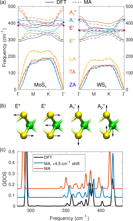
Figure 1: (a) Phonon dispersion curves of pristine MoS₂ (left) and WS₂ (right) calculated either self-consistently using DFT (solid lines) or using the mass-approximation (dashed lines). Dots denote experimental values obtained from Raman spectroscopy Zhang et al. (2015); Livneh and Spanier (2015). (b) Schematic representation of Mo (green) and S (yellow) atoms vibrations in different optical phonon modes. (c) GDOS from 3$\times$3 SQS of Mo_0.56W_0.44S₂, either calculated fully with DFT or using the mass approximation.

We start by benchmarking our computational scheme with respect to the mass-approximation. We show in Fig. 1(a) the phonon dispersion curves of MoS₂ and WS₂ calculated with DFT and the mass-approximated versions (i.e., using the MoS₂ FC matrix but substituting the mass of Mo by that of W and vice versa). The dispersions of the bands are captured very well with MA as are the acoustic mode frequencies. There is a nearly constant downshift of the optical mode frequencies of WS₂ by about 10 cm^-1 with respect to self-consistent WS₂ calculation, and vice versa an upshift in MoS₂ frequencies if using WS₂ FC with Mo mass, suggesting that W-S bonds are slightly stronger than Mo-S bonds. In the following of this work, we have chosen to use the MoS₂ force constants. With this choice, when comparing to the experimental values for the two Raman-active modes, E^′ and A${}_{1}^{\prime}$, our calculated frequencies are slightly overestimated for MoS₂ and slightly underestimated for WS₂ when compared to full DFT calculation.

The effect of MA is further illustrated in Fig. 1(c) in the case of the (Mo,W)S₂ alloy supercell. The structural models used in the alloy calculations are constructed using the special quasirandom structures (SQS) method Zunger et al. (1990). As seen in Fig. 1(c) for 3$\times$3 Mo_0.56W_0.44S₂ SQS, the MA frequencies are downshifted throughout the spectrum, similar to the pristine systems. To allow for a better comparison with the DFT results, we also show a spectrum shifted up by 4.5 cm^-1 (from the alloy composition times 10 cm^-1), after which the main peaks (E^′, A${}_{1}^{\prime}$) and the high-frequency part of the E^′ feature (from 350 to 400 cm^-1) agree very well. The low-frequency part of E^′′ features has still a too low frequency, which is due to the fact that these modes are localized to W atoms, as will be seen later.

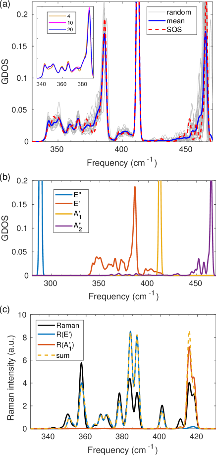
Figure 2: (a) GDOS from 20 random atomic configurations for Mo_0.56W_0.44S₂ (gray lines) together with their average (blue, solid line). GDOS for the 12$\times$12 SQS supercell is also shown for comparison. Inset: Comparison of results when the averaging is done over 4, 10, or 20 configurations. (b) Primitive cell eigenmode projected GDOS for the SQS cell [same as in panel (a)]. (c) Raman spectra from full DFT calculation for the 3$\times$3 SQS supercell of Mo_0.56W_0.44S₂ compared to its RGDOS, and the contributions to it from the two primitive cell eigenmodes.

Next, we inspect the importance of statistical sampling. We use the supercell comprising 12$\times$12 primitive cells and 20 different random configurations (not SQS) for each composition. Fig. 2(a) shows the spectra from all the 20 configurations and the averaged spectra. The large variation in the single spectra indicates that 12$\times$12 supercell is still not quite large enough to correctly describe the alloy with a single supercell. As shown in the inset, averaging over just 4 configurations yields a spectrum that is already quite similar to that from 20 configurations. In addition, we compare the averaged spectrum to that of a SQS model created within the 12$\times$12 supercell. We consider pairs up to 8 Å (three effective cluster interaction (ECI) parameters) and three-body clusters up to 4 Å (2 ECI). The SQS performs better than the different random configurations, but fails to correctly capture the smooth broadening of the main peaks, instead yielding more spiked features. This originates from the coarseness of the mesh of k-points that folds into the $\Gamma$-point in small supercell calculations. Note, that the A${}_{1}^{\prime}$ mode is in practice completely unaffected by the mixing, as it only involves movement of the chalcogen atoms and the metal atoms are fixed (see Fig. 1(b)).

Finally, we benchmark the eigenmode-projection scheme. First, we illustrate in Fig. 2(b) the eigenmode contributions in the case of 12$\times$12 SQS. In H-MoWS₂ alloy, the modes remain fairly separated in frequency and thus the resulting Raman spectra could be fairly safely evaluated from just the GDOS. On the other hand, the projection scheme provides further insight in to the origin of the spectral features. For instance, the bump at around 400 cm^-1 originates from the E^′ mode and not from the A${}_{1}^{\prime}$ mode. Also, at large W concentration, the A${}_{2}^{\prime\prime}$ features start to overlap with the E^′/A${}_{1}^{\prime}$ features, as will be seen in the Results section. Moreover, we need to compare how well the approximated Raman spectra match to explicit Raman calculations. For this we need to adopt a smaller system, and since this is only for benchmarking purposes we can take a 3$\times$3 supercell, again created using the SQS scheme. The RGDOS captures surprisingly well all the features of the full Raman calculation, as shown in Fig. 2(c). Especially, the peak shapes/structures are correctly reproduced, even if some intensities differ with the most significant discrepancy occuring near 385 cm^-1. From the comparison of the spectra in Figs. 2(b) and (c) it is again obvious that 3$\times$3 SQS cannot describe properly the Raman spectrum of the random alloy.

We have demonstrated that large supercells are needed to properly describe the phonon spectra of random alloys and that RGDOS can be used to give a good estimate of the Raman spectrum. While the mass approximation may produce some inaccuracies with the peak positions, we feel that this is acceptable tradeoff for the ability to correctly describe the random alloy. In the following, the results for the alloys are obtained by averaging over 20 configurations of the 12$\times$12 supercell and using the eigenmode-projection. In few cases, the analysis of the results is done using the SQS structure, which results in great simplification.

III Results

III.1 H-(Mo,W)S₂

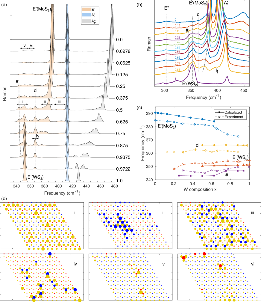
Figure 3: (a) RGDOS for Mo_1-xW_xS₂ alloy, $x$ ranges from 0 to 1. The total RGDOS is shown with solid black line. The contributions from E^′, A${}_{1}^{\prime}$, and A${}_{2}^{\prime\prime}$ modes are shown by yellow, blue, and grey shaded areas, repectively. (b) Experiments, adapted from Ref. Chen et al., 2014. (c) The calculated compositional dependence of the Raman peaks frequencies vs. the experimental counterparts. (d) Illustration of selected eigenmodes (i - iv) from (a). The blue, red, and yellow symbols correspond to Mo, W, and S atoms, respectively. The atoms are positioned in the supercell and the magnitude of symbols is propertional to the amplitude of vibrations.

The simulated Raman spectra for H-(Mo,W)S₂ monolayer as a function of the composition are shown in Fig. 3(a), and which can be compared to experimental Raman spectra shown in Fig. 3(b) (from Ref. Chen et al., 2014). The calculated A${}_{2}^{\prime\prime}$ mode, although not Raman-active, is also shown, since it is infrared active and shows large changes with the composition. To make it visible in the simulated spectra we use the same Raman tensor as for A${}_{1}^{\prime}$. The experimental and calculated peak positions are collected in Fig. 3(c). The A${}_{1}^{\prime}$ mode consists of only chalcogen movement and thus in our mass approximation approach this mode remains strictly constant. Also E^′′ is unaffected by the MA and thus not shown in the calculated spectra, although its activation due to disorder is visible in the experimental spectra.

Overall a good agreement with the experiment is observed for the number of peaks as well as their positions: (i) For the E^′ mode, we confirm pronounced two-mode behavior with the separate MoS₂- and WS₂-derived peaks. (ii) There is a clear downshift of the E^′(MoS₂) peak, whereas the E^′(WS₂) peak remains nearly constant in energy. In experiment, at large W concentration the MoS₂-derived peak broadens and possibly mixes with the d feature (marked d, as it was denoted “disorder-related mode” in Ref. Chen et al., 2014). (iii) There are two additional features around the WS₂ peak: one at about 345 cm^-1 (marked #) and one at about 360 cm^-1 (unmarked) in calculations. The latter is difficult to observe in Fig. 3(b), but evident in the line shape fits in Ref. Chen et al., 2014. (iv) Both in experiment and theory, at small W concentrations, the W-derived features form a broad plateau below the E^′(MoS₂) peak with no particularly distinct peaks. (v) A small bump develops between the E^′(MoS₂)and A${}_{1}^{\prime}$ peaks, which originates fully from the E^′-mode. While in calculations it prevails at intermediate concentrations, in experiments this is only clearly visible at the W-rich side, and thus it is not clear if their origin is the same.

In order to understand the atomic origin of these peaks, we illustrate the eigenvectors from selected cases in Fig. 3(d), where the sizes of the circles at the position of atom $k$ correspond to the eigenvector weighted by the $\Gamma$-point projection $|\mathbf{v}(k0)|^{2}\cdot w^{2}$ summed over all modes within the selected range of frequencies marked in Fig. 3(a). As expected, the modes corresponding to MoS₂- and WS₂-derived peaks are localized around Mo and W atoms, respectively. The broader feature between E^′ and A${}_{1}^{\prime}$ appears to be localized at the edges of the Mo-regions (panel iii). The “disorder-related mode” is not very visible at $x=0.5$, but at $x=0.875$ our analysis clearly shows that it is localized to isolated Mo atoms (panel iv).

The smaller peaks around it, on the other hand, are localized to Mo-clusters (not shown), whose density at W-rich samples is naturally small. The peaks denoted by $\#$-modes appear visually very similar to the main WS₂-derived modes and thus we think that this shoulder just originates from asymmetrical broadening of the WS₂-peak. On the other hand, this mode was assigned to 2LA(M) in Ref. Chen et al., 2014). Our calculated LA(M) frequency for WS₂ is 177 cm^-1, yielding 2LA(M) at 354 cm^-1, and thus lies slightly above the E^′(WS₂)-peak in our calculations, but could also be slightly below the E^′(WS₂)-peak in experiments. Since we here only simulate the first-order Raman scattering, we know that the shoulder in calculations contains no 2LA(M) contribution, but naturally we cannot exclude such additional contribution in the experimental spectra.

III.2 T’-(Mo,W)Te₂

We next study T’-(Mo,W)Te₂ alloy, which is computationally a significantly more challenging case, since (i) the unit cell is larger and has lower symmetry than the H-phase, thus leading to larger number of displacements in pristine system, (ii) it is (semi-)metallic, necessitating the use of large k-point meshes. The latter also means that the Raman spectra will necessarily be resonant, but the evaluation of the Raman tensor from the change of macroscopic dielectric constant assumes non-resonant conditions. Resonant Raman tensors can be used just as well in our approach for simulated Raman spectra (Eq. 9), but their evaluation from first principles is again step up in computational complexity and moreover makes the tensors frequency-dependent. To avoid these problems, we here use the non-resonant Raman tensors, which are moreover normalized in order to better highlight all the Raman-active features, although this means that the relative intensities of the peaks are not correctly captured. The classification of the $\Gamma$-point vibrations, $\Gamma_{C_{i}}$ = 9 A_g + 9 A_u, shows that half (A_g) of the modes are Raman-active. These modes can be arranged in two groups: modes vibrating along the direction of the zigzag Mo/W chain, denoted by A${}_{g}^{z}$, and modes vibrating perpendicular to the zigzag chain, denoted by A${}_{g}^{a}$.

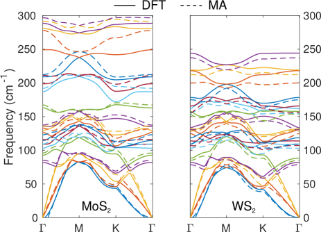
Figure 4: Phonon dispersion curves of pristine MoTe₂ (left) and WTe₂ (right) calculated either self-consistently using DFT (solid lines) or using mass-approximation (dashed lines).

Phonon dispersion curves calculated by DFT and by mass approximation are shown in Fig. 4. We again observe that frequencies from MA are shifted down by about 10 cm^-1 in WTe₂, but the order and dispersion of the bands is captured well. The only clear deviation occurs for WTe₂ around 220 cm^-1 at the $\Gamma$-point, where the quasi-degenerate Raman active modes from the DFT calculation breaks into two modes at 200 cm^-1 and 212 cm^-1 from the MA calculation, echoing the splitting observed in MoTe₂ at 250 cm^-1 and 280 cm^-1. This feature is observed in experiment for bulk (Mo,W)Te₂ Joshi et al. (2016a). It is worth noting that the lattice constants of MoTe₂ (3.37 Å, 7.15 Å) and WTe₂ (3.42 Å, 7.12Å) are not quite as close as those of the parent compounds in H-(Mo,W)S₂.

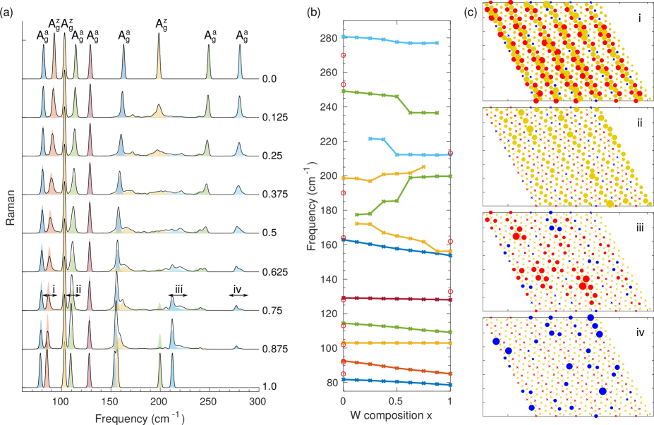
Figure 5: (a) RGDOS for T’-(Mo,W)Te₂. The total RGDOS is shown with solid black line. The shaded areas show contributions from the projection to eigenmodes of the pristine T^′-MoTe₂. The modes are colored sequentially (and loops once). (b) Evolution of the peak maxima positions for Mo_1-xW_xTe₂ alloys. Experimental data (red open circles) are taken from Refs. Jiang et al. (2016); Chen et al. (2017). (c) Illustration of selected SC eigenmodes from the $x=0.75$ case, as indicated in (a). The SC eigenmodes within the frequency range are weighted by the projection to the dominant PC eigenmode. The blue, red, and yellow symbols correspond to Mo, W, and Te atoms, respectively.

The calculated RGDOS for the monolayer T’-(Mo,W)Te₂ alloy as a function of composition are shown in Fig. 5(a) and the peak positions are collected in Fig. 5(b). We remind, that while in H-(Mo,W)S₂ the alloy modes could be easily assigned to the pristine modes from which they originated thanks to the large separation in frequency, here due to the large number of modes, the mixing is more complicated and thus the eigenmode-projection is necessary to distinguish between the Raman-active and -inactive features. The projection scheme allows us to distinguish the origins of each peak in terms of the primitive cell eigenmodes, revealing that the ordering of the modes is retained in the same order throughout the alloys. The eigenvectors of these modes in the parent phases have been illustrated in several previous works Jiang et al. (2016); Kim et al. (2016); Beams et al. (2016); Chen et al. (2016); Grzeszczyk et al. (2016); Zhang et al. (2016b); Wang et al. (2017); Chen et al. (2017), and are not repeated here. Nevertheless, they show that the six lowest frequency modes are mostly localized to Te atoms, and the three high frequency modes to Mo/W atoms. Consequently, the six lowest frequency modes exhibit single-mode behavior and the three high frequency modes two-mode behavior, reflecting the fact that alloying is carried out in the metal sublattice. Among the six lowest frequency modes that exhibit the single mode behavior, the third one is silent in the metal sublattice and the fifth one nearly silent Chen et al. (2017), and thus they show very little changes upon alloying. There are also clear differences in the degree of the alloying-induced broadening of the other four peaks, with the first one showing least broadening, the second one the strongest broadening, and the fourth and sixth modes falling in between. Fig. 5(c) illustrates the second and fourth modes of the x=0.75 alloy. The fourth mode (panel ii) is localized very clearly only on the Te atoms and mostly on the rows with long metal-metal distance, whereas the second mode has also weight on the metal atoms and is mostly localized on the rows with short metal-metal distance.

The last three modes in Fig. 5(a) show a very clear two-mode behavior with splitting into MoTe₂ and WTe₂-like modes at intermediate alloy concentrations. The eigenvectors in Fig. 5(c) show that these modes are localized almost completely on the metal atoms and the two-mode behavior reflects the localization around Mo and W atoms. The eigenmode projections illustrated in Fig. 5(c) are found to provide additional insight into the peak origins. For instance, there is a mode at 200 cm^-1 in both the MoTe₂ and WTe₂ phases, but the projections reveal that they correspond to different modes. Somewhat similarly, the 160 cm^-1 peak in WTe₂ is seen to contain two modes, which in the MoTe₂ region are located at 160 cm^-1 and 200 cm^-1.

Comparison to experimental results is hindered by the fact, that to the best of our knowledge, all the experimental T’-Mo_(1-x)W_xTe₂ alloy results are from bulk samples Revolinsky and Beerntsen (1964); Oliver et al. (2017); Lv et al. (2017); Rhodes et al. (2017). Monolayer data is only available for pure MoTe₂ and WTe₂ Chen et al. (2017); Jiang et al. (2016); Kim et al. (2016). Naturally, there exists also a large body of data for pure bulk or few-layer phases Joshi et al. (2016b); Beams et al. (2016); Ma et al. (2016); Chen et al. (2016); Grzeszczyk et al. (2016); Wang et al. (2017); Zhang et al. (2016b). Although the bulk and monolayer frequencies are generally fairly close, to facilitate a proper comparison, in Fig. 5(b) we only show the available monolayer results for MoTe₂ and WTe₂. For the low-frequency modes in MoTe₂ and WTe₂, calculated and experimental frequencies agree very well. The agreement deteriorates for high-frequency modes, but the experimental and calculated peaks can still be mapped. Also the ordering of the A${}_{g}^{a}$ and A${}_{g}^{z}$ modes is correctly reproduced. When comparing to the bulk alloy results, our calculations indicate that the reported disorder-activated modes around 180 cm^-1 and 202 cm^-1 Oliver et al. (2017), can be a mix of the last three high-frequency modes and can be tuned by varying composition. Our calculations produce a large number of small peaks at these frequencies, with contributions from all the three high-frequency modes, but we do not obtain one or two prominent peaks. This might be caused by normalization of Raman tensors in our simulated spectra. The peak at 130 cm^-1 in MoTe₂ was found to split into two peaks separated by about 3 cm^-1 upon increasing the W concentration Oliver et al. (2017); Lv et al. (2017), and was assigned to mixing in Ref. Oliver et al., 2017 and to a phase change from monoclinic to orthorhombic lattice in Refs. Lv et al. (2017); Chen et al. (2016). Since this peak is silent in the metal sublattice, it shows no alloying-induced splitting nor even any broadening in our calculations, and thus our calculations do not support the assignment to mixing. For the highest frequency mode, our calculations correctly capture the broadening toward higher frequencies on both the MoTe₂ and WTe₂ regions Oliver et al. (2017).

III.3 Impurities in H-MoS₂

The Raman signatures can be used to identify impurities at small concentrations (small with respect to alloying, i.e., within few percent). In some instances, as seen also in the previous sections, impurities can produce very distinct new peaks, broaden existing peaks, or result in very broad features. In this section, we insert a small number of impurity atoms into the lattice and examine the trends in the changes of the Raman spectra. The mass approximation limits our study to cases where chemical bonding upon substitution is expected to remain fairly similar. To this end, we either replace the Mo atom by other transition metal element or the S atom by an atom from the nitrogen, oxygen, or fluorine groups. Clearly, this is expected to work best for the elements in the same column in the periodic table and worsen the further away from it. The small impurity concentration helps to avoid problems with the large strain. For the calculations, we here adopt a slightly simplified procedure, where we simply take the 5$\times$5 supercell with a single impurity. This is sufficiently large to describe the localized modes, and while the peak broadenings would not be correctly described, there are very little changes in the position and broadening of the main peaks in these dilute cases.

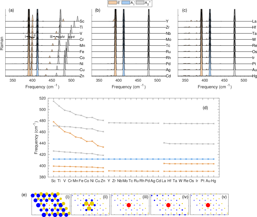
Figure 6: (a-c) RGDOS for impurities in the Mo site in MoS₂, grouped by the rows in the periodic table. (d) Positions of the peak maxima extracted from panels (a-c). (e) Selected eigenmodes from the Cr case. The blue, red, and yellow symbols correspond to Mo, Cr, and S atoms, respectively.

The RGDOS for the Mo-site impurities are shown in Fig. 6(a-c). One impurity in 25 lattice sites corresponds to the $4\%$ impurity concentration. The behavior is clearly different for 3d, 4d, and 5d transitional metal impurities. Following the impurity masses, the additional impurity induced peaks are at highest frequencies for the 3d elements and at lowest frequencies for 5d elements, whereas the 4d impurities show very little new features. In case of the 3d elements, there is a pronounced splitting between the E^′ and A${}_{2}^{\prime\prime}$ modes and an additional, mostly E^′-derived, mode between the two. We note again that A${}_{2}^{\prime\prime}$ mode is not Raman-active, and only shown here for reference. The eigenmodes are shown in Fig. 6(e). Not surprisingly, the main peak is localized in the MoS₂ regions (panel i) The second E^′ feature is localized around the impurity (panel ii) and the last one strictly at the impurity (panel iii). This last E^′ peak should have appreciable Raman intensity and frequency that sensitively depends on the transition metal impurity and thus seems to provide the most effective impurity signature. For the two A${}_{2}^{\prime\prime}$-derived peaks, the lower frequency mode is localized in the MoS₂ regions (panel iv, the Cr atom shows intense due to its small mass, but all Mo atoms are also active) and the higher frequency one around the impurity (panel v).

Very little happens with the 4d impurities, only a small shift of the main E^′ mode together with slight broadening, stemming from the small (relative) change of the mass. All the 5d impurities show features similar to the (Mo,W)S₂ alloy considered previously: a broad set of weak features at 350–400 cm^-1 and one peak between E^′ and A${}_{1}^{\prime}$ peaks. For the two eigenmodes shown in Fig. 3(d) (panels v,vi), despite having clearly different frequencies, they have fairly similar eigenvectors. Since the MoS₂ E^′′, A₁, and A${}_{2}^{\prime\prime}$ modes at the K and M points largely fall at frequencies between 350 and 400 cm^-1, we think these impurity modes have large contributions from the off-$\Gamma$ k-points and only a small $\Gamma$-point, Raman-active contribution. In essence, these impurities lead to mixing of the vibrational modes at different q-points of the primitive cell BZ. No pronounced features are observed at low frequencies, and there are no gap states.

Overall, it appears that it should be possible to resolve the presence of even fairly dilute concentration of 3d transition metal impurities in MoS₂ from the splitting of the E^′ peak, possibly even with the elemental precision, although the absolute values given here may suffer from the limitations of the mass approximation. Dilute concentration 4d impurities are expected to be largely invisible in Raman, whereas 5d impurities might show up in Raman but their identification can be difficult.

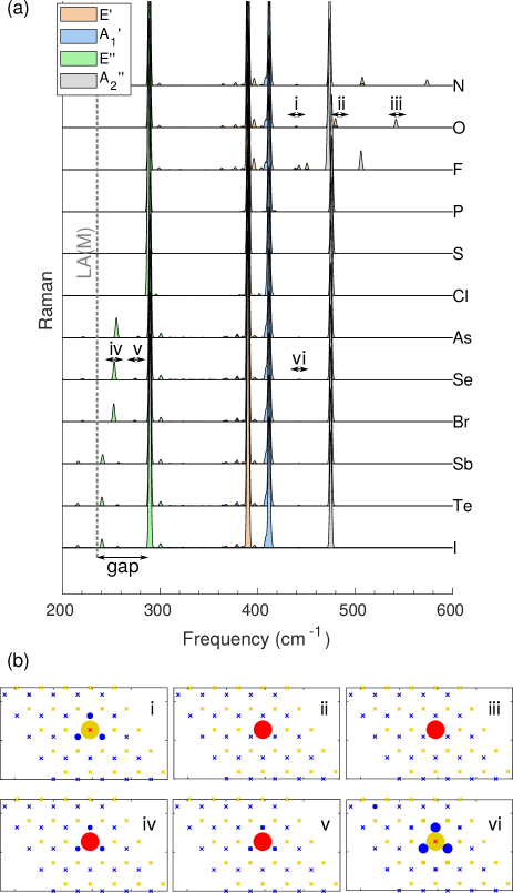
Figure 7: (a) RGDOS for impurities in the S site in MoS₂. The LA(M) frequency from pristine MoS₂ and the gap in the phonon structure are also indicated. (b) Selected eigenmodes for the O and Se impurity systems. The blue, red, and yellow symbols correspond to Mo, O/Se, and S atoms, respectively.

The RGDOS for the S-site impurities in MoS₂ are shown in Fig. 7(a). One impurity in 50 lattice sites corresponds to $2\%$ impurity concentration. Again, lighter impurities lead to additional peaks at higher frequencies and heavier impurities at lower frequencies, but the features that are most likely to be observed in experiments are those falling above the A${}_{2}^{\prime\prime}$ mode or inside the gap between E^′′ mode and the LA(M) edge. In fact, such features have been reported in the literature for MoS₂ with light Se alloying at about 270 cm^-1 Li et al. (2014); Su et al. (2014b); Mann et al. (2014); Feng et al. (2015) and with light Te alloying at about 243 cm^-1 Yin et al. (2018), agreeing well with our calculations.

O and Se impurities in MoS₂ are chosen as representative examples to be discussed in more detail. Selected eigenvectors of these impurity systems are presented in Fig. 7(b). In the case of the O impurity, the feature (ii) just above A${}_{2}^{\prime\prime}$ is mainly derived from E^′ with a small E^′′ contribution and it should thus be visible in Raman measurements. The high frequency feature (iii) is mostly of A${}_{2}^{\prime\prime}$ type, but it contains also an appreciable A${}_{1}^{\prime}$ contribution and thus could also be visible. In the case of the Se impurity, there are two features in the gap, with the lower one (iv) derived mostly out of E^′′ with some E^′, and the higher one (v) mostly from the pristine A${}_{1}^{\prime}$ mode with some A${}_{2}^{\prime\prime}$ character. Finally, we mention the features (i) and (vi), which are localized mostly at the S atom on the opposite side of the layer from the impurity atom and thus they also have the same frequency, independent of the impurity element. While this feature is barely visible in the simulated spectrum, it is derived mostly from the pristine A${}_{1}^{\prime}$ mode and thus could be observable.

IV Conclusions

We have devised an efficient computational method to simulate Raman spectra of large systems, being especially applicable to alloys and also systems with small number of defects. The method is based on the projection of vibrational eigenvectors of the supercell to the eigenvectors from the primitive cell and using them as weights in summing over the Raman tensors calculated at the primitive cell. We moreover used mass approximation to rapidly evaluate the vibrational modes in the supercell. We applied the method to two different transition metal dichalcogenide monolayer alloys, H-(Mo,W)S₂ and T’-(Mo,W)Te₂, and to impurities in H-MoS₂. The accuracy of the method was validated in the case of H-(Mo,W)S₂ alloy through comparison to the available experimental reports. T’-(Mo,W)Te₂ and impurity cases are used to (i) demonstrate the wider applicability of the method and (ii) provide predictions in few technologically relevant systems. We note that in addition to yielding the simulated Raman spectra, the projection scheme also provides a powerful tool for analyzing the origin of the Raman-active features. The method presented here is not limited to 2D materials, and is applicable to various other bulk and low-dimensional systems.

References

- Nicolosi et al. (2013) V. Nicolosi, M. Chhowalla, M. G. Kanatzidis, M. S. Strano, and J. N. Coleman, “Liquid Exfoliation of Layered Materials,” Science 340, 1420 (2013).
- Lebègue et al. (2013) S. Lebègue, T. Björkman, M. Klintenberg, R. M. Nieminen, and O. Eriksson, “Two-Dimensional Materials from Data Filtering and Ab Initio Calculations,” Phys. Rev. X 3, 031002 (2013).
- Mounet et al. (2018) N. Mounet, M. Gibertini, P. Schwaller, D. Campi, A. Merkys, A. Marrazzo, T. Sohier, I. E. Castelli, A. Cepellotti, G. Pizzi, and N. Marzari, “Two-Dimensional Materials from High-Throughput Computational Exfoliation of Experimentally Known Compounds,” Nature Nanotechnology 13, 246–252 (2018).
- Revolinsky and Beerntsen (1964) E. Revolinsky and D. Beerntsen, “Electrical Properties of the MoTe2 - WTe2 and MoSe2 - WSe2 Systems,” Journal of Applied Physics 35, 2086–2089 (1964).
- Srivastava et al. (1997) S. K. Srivastava, T. K. Mandal, and B. K. Samantaray, “Studies on Layer Disorder, Microstructural Parameters and Other Properties of Tungsten-Substitued Molybdenum Disulfide, Mo1-xWxS2 (),” Synthetic Metals 90, 135 – 142 (1997).
- Chen et al. (2013) Y. Chen, J. Xi, D. O. Dumcenco, Z. Liu, K. Suenaga, D. Wang, Z. Shuai, Y.-S. Huang, and L. Xie, “Tunable Band Gap Photoluminescence from Atomically Thin Transition-Metal Dichalcogenide Alloys,” ACS Nano 7, 4610–4616 (2013).
- Komsa and Krasheninnikov (2012) H.-P. Komsa and A. V. Krasheninnikov, “Two-Dimensional Transition Metal Dichalcogenide Alloys: Stability and Electronic Properties,” The Journal of Physical Chemistry Letters 3, 3652–3656 (2012).
- Kang et al. (2013) J. Kang, S. Tongay, J. Li, and J. Wu, “Monolayer Semiconducting Transition Metal Dichalcogenide Alloys: Stability and Band Bowing,” Journal of Applied Physics 113, 143703 (2013).
- Li et al. (2014) H. Li, X. Duan, X. Wu, X. Zhuang, H. Zhou, Q. Zhang, X. Zhu, W. Hu, P. Ren, P. Guo, L. Ma, X. Fan, X. Wang, J. Xu, A. Pan, and X. Duan, “Growth of Alloy MoS2xSe2(1-x) Nanosheets with Fully Tunable Chemical Compositions and Optical Properties,” Journal of the American Chemical Society 136, 3756–3759 (2014).
- Mann et al. (2014) J. Mann, Q. Ma, P. M. Odenthal, M. Isarraraz, D. Le, E. Preciado, D. Barroso, K. Yamaguchi, G. von Son Palacio, A. Nguyen, T. Tran, M. Wurch, A. Nguyen, V. Klee, S. Bobek, D. Sun, T. F. Heinz, T. S. Rahman, R. Kawakami, and L. Bartels, “2-Dimensional Transition Metal Dichalcogenides with Tunable Direct Band Gaps: MoS2(1-x)Se2x Monolayers,” Advanced Materials 26, 1399–1404 (2014).
- Rigosi et al. (2016) A. F. Rigosi, H. M. Hill, K. T. Rim, G. W. Flynn, and T. F. Heinz, “Electronic Band Gaps and Exciton Binding Energies in Monolayer MoxW1-xS2 Transition Metal Dichalcogenide Alloys Probed by Scanning Tunneling and Optical Spectroscopy,” Phys. Rev. B 94, 075440 (2016).
- Wang et al. (2015a) G. Wang, C. Robert, A. Suslu, B. Chen, S. Yang, S. Alamdari, I. C. Gerber, T. Amand, X. Marie, S. Tongay, and B. Urbaszek, “Spin-Orbit Engineering in Transition Metal Dichalcogenide Alloy Monolayers,” Nat Commun 6, 10110 (2015a).
- Gu and Yang (2016) X. Gu and R. Yang, “Phonon Transport in Single-Layer Mo1-xWxS2 Alloy Embedded with WS2 Nanodomains,” Phys. Rev. B 94, 075308 (2016).
- Qian et al. (2018a) X. Qian, P. Jiang, P. Yu, X. Gu, Z. Liu, and R. Yang, “Anisotropic Thermal Transport in van der Waals Layered Alloys WSe2(1-x)Te2x,” Applied Physics Letters 112, 241901 (2018a).
- Huang et al. (2015) B. Huang, M. Yoon, B. G. Sumpter, S.-H. Wei, and F. Liu, “Alloy Engineering of Defect Properties in Semiconductors: Suppression of Deep Levels in Transition-Metal Dichalcogenides,” Phys. Rev. Lett. 115, 126806 (2015).
- Yao et al. (2016) J. Yao, Z. Zheng, and G. Yang, “Promoting the Performance of Layered-Material Photodetectors by Alloy Engineering,” ACS Applied Materials & Interfaces 8, 12915–12924 (2016).
- Kiran et al. (2014) V. Kiran, D. Mukherjee, R. N. Jenjeti, and S. Sampath, “Active Guests in the MoS2/MoSe2 Host Lattice: Efficient Hydrogen Evolution Using Few-Layer Alloys of MoS2(1-x)Se2x,” Nanoscale 6, 12856–12863 (2014).
- Wang et al. (2015b) L. Wang, Z. Sofer, J. Luxa, and M. Pumera, “MoxW1-xS2 Solid Solutions as 3D Electrodes for Hydrogen Evolution Reaction,” Advanced Materials Interfaces 2, 1500041 (2015b).
- Cazalilla et al. (2014) M. A. Cazalilla, H. Ochoa, and F. Guinea, “Quantum Spin Hall Effect in Two-Dimensional Crystals of Transition-Metal Dichalcogenides,” Phys. Rev. Lett. 113, 077201 (2014).
- Qian et al. (2014) X. Qian, J. Liu, L. Fu, and J. Li, “Quantum Spin Hall Effect in Two-Dimensional Transition Metal Dichalcogenides,” Science 346, 1344–1347 (2014).
- Sun et al. (2015) Y. Sun, S.-C. Wu, M. N. Ali, C. Felser, and B. Yan, “Prediction of Weyl Semimetal in Orthorhombic MoTe2,” Phys. Rev. B 92, 161107 (2015).
- Huang et al. (2016) L. Huang, T. M. McCormick, M. Ochi, Z. Zhao, M.-T. Suzuki, R Arita, Y. Wu, D. Mou, H. Cao, J. Yan, N. Trivedi, and A. Kaminski, “Spectroscopic Evidence for a Type II Weyl Semimetallic State in MoTe2,” Nat Mater 15, 1155–1160 (2016).
- Duerloo and Reed (2016) K.-A. N. Duerloo and E. J. Reed, “Structural Phase Transitions by Design in Monolayer Alloys,” ACS Nano 10, 289–297 (2016).
- Zhang et al. (2016a) C. Zhang, S. KC, Y. Nie, C. Liang, W. G. Vandenberghe, R. C. Longo, Y. Zheng, F. Kong, S. Hong, R. M. Wallace, and K. Cho, “Charge Mediated Reversible Metal-Insulator Transition in Monolayer MoTe2 and WxMo1-xTe2 Alloy,” ACS Nano 10, 7370–7375 (2016a).
- Fei et al. (2018) Z. Fei, W. Zhao, T. A. Palomaki, B. Sun, M. K. Miller, Z. Zhao, J. Yan, X. Xu, and D. H. Cobden, “Ferroelectric Switching of a Two-Dimensional Metal,” Nature 560, 336–339 (2018).
- Chen et al. (2014) Y. Chen, D. O. Dumcenco, Y. Zhu, X. Zhang, N. Mao, Q. Feng, M. Zhang, J. Zhang, P.-H. Tan, Y.-S. Huang, and L. Xie, “Composition-Dependent Raman Modes of Mo1-xWxS2 Monolayer Alloys,” Nanoscale 6, 2833–2839 (2014).
- Liu et al. (2014) H. Liu, K. K. A. Antwi, S. Chua, and D. Chi, “Vapor-Phase Growth and Characterization of Mo1-xWxS2 () Atomic Layers on 2-Inch Sapphire Substrates,” Nanoscale 6, 624–629 (2014).
- Park et al. (2018) J. Park, M. S. Kim, B. Park, S. H. Oh, S. Roy, J. Kim, and W. Choi, “Composition-Tunable Synthesis of Large-Scale Mo1–xWxS2 Alloys with Enhanced Photoluminescence,” ACS Nano 12, 6301–6309 (2018).
- Tongay et al. (2014) S. Tongay, D. S. Narang, J. Kang, W. Fan, C. Ko, A. V. Luce, K. X. Wang, J. Suh, K. D. Patel, V. M. Pathak, J. Li, and J. Wu, “Two-Dimensional Semiconductor Alloys: Monolayer Mo1-xWxSe2,” Applied Physics Letters 104, 012101 (2014).
- Zhang et al. (2014) M. Zhang, J. Wu, Y. Zhu, D. O. Dumcenco, J. Hong, N. Mao, S. Deng, Y. Chen, Y. Yang, C. Jin, S. H. Chaki, Y.-S. Huang, J. Zhang, and L. Xie, “Two-Dimensional Molybdenum Tungsten Diselenide Alloys: Photoluminescence, Raman Scattering, and Electrical Transport,” ACS Nano 8, 7130–7137 (2014).
- Feng et al. (2015) Q. Feng, N. Mao, J. Wu, H. Xu, C. Wang, J. Zhang, and L. Xie, “Growth of MoS2(1-x)Se2x () Monolayer Alloys with Controlled Morphology by Physical Vapor Deposition,” ACS Nano 9, 7450–7455 (2015).
- Su et al. (2014a) S.-H. Su, Y.-T. Hsu, Y.-H. Chang, M.-H. Chiu, C.-L. Hsu, W.-T. Hsu, W.-H. Chang, J.-H. He, and L.-J. Li, “Band Gap-Tunable Molybdenum Sulfide Selenide Monolayer Alloy,” Small 10, 2589–2594 (2014a).
- Wen et al. (2017) W. Wen, Y. Zhu, X. Liu, H.-P. Hsu, Z. Fei, Y. Chen, X. Wang, M. Zhang, K.-H. Lin, F.-S. Huang, Y.-P. Wang, Y.-S. Huang, C.-H. Ho, P.-H. Tan, C. Jin, and L. Xie, “Anisotropic Spectroscopy and Electrical Properties of 2D ReS2(1-x)Se2x Alloys with Distorted 1T Structure,” Small 13, 1603788–n/a (2017), 1603788.
- Dumcenco et al. (2010) D.O. Dumcenco, K.Y. Chen, Y.P. Wang, Y.S. Huang, and K.K. Tiong, “Raman Study of 2H-Mo1-xWxS2 Layered Mixed Crystals,” Journal of Alloys and Compounds 506, 940 – 943 (2010).
- Oliver et al. (2017) S. M. Oliver, R. Beams, S. Krylyuk, I. Kalish, A. K Singh, A. Bruma, F. Tavazza, J. Joshi, I. R. Stone, S. J. Stranick, A. V. Davydov, and P. M. Vora, “The Structural Phases and Vibrational Properties of Mo1-xWxTe2 Alloys,” 2D Materials 4, 045008 (2017).
- Lv et al. (2017) Y.-Y. Lv, L. Cao, X. Li, B.-B. Zhang, K. Wang, B. Pang, L. Ma, D. Lin, S.-H. Yao, J. Zhou, Y. B. Chen, S.-T. Dong, W. Liu, M.-H. Lu, Y. Chen, and Y.-F. Chen, “Composition and Temperature-Dependent Phase Transition in Miscible Mo1-xWxTe2 Single Crystals,” Scientific Reports 7, 44587 (2017).
- Molina-Sánchez and Wirtz (2011) A. Molina-Sánchez and L. Wirtz, “Phonons in single-layer and few-layer mos2 and ws2,” Phys. Rev. B 84, 155413 (2011).
- Zhang et al. (2015) X. Zhang, X.-F. Qiao, W. Shi, J.-B. Wu, D.-S. Jiang, and P.-H. Tan, “Phonon and Raman Scattering of Two-Dimensional Transition Metal Dichalcogenides From Monolayer, Multilayer to Bulk Material,” Chem. Soc. Rev. 44, 2757–2785 (2015).
- Saito et al. (2016) R. Saito, Y. Tatsumi, S. Huang, X. Ling, and M. S. Dresselhaus, “Raman Spectroscopy of Transition Metal Dichalcogenides,” Journal of Physics: Condensed Matter 28, 353002 (2016).
- Parkin et al. (2016) W. M. Parkin, A. Balan, L. Liang, P. M. Das, M. Lamparski, C. H. Naylor, J. A. Rodríguez-Manzo, A. T. C. Johnson, V. Meunier, and M. Drndić, “Raman Shifts in Electron-Irradiated Monolayer MoS2,” ACS Nano 10, 4134–4142 (2016).
- Bae et al. (2017) S. Bae, N. Sugiyama, T. Matsuo, H. Raebiger, K.-I. Shudo, and K. Ohno, “Defect-Induced Vibration Modes of Ar+-Irradiated MoS2,” Phys. Rev. Applied 7, 024001 (2017).
- Baroni et al. (1990) S. Baroni, S. de Gironcoli, and P. Giannozzi, “Phonon Dispersions in GaxAl(1-x)As alloys,” Phys. Rev. Lett. 65, 84–87 (1990).
- Menéndez (2000) J. Menéndez, “Characterization of Bulk Semiconductors Using Raman Spectroscopy,” in Raman Scattering in Materials Science, edited by Willes H. Weber and Roberto Merlin (Springer Berlin Heidelberg, Berlin, Heidelberg, 2000) pp. 55–103.
- Allen et al. (2013) P. B. Allen, T. Berlijn, D. A. Casavant, and J. M. Soler, “Recovering Hidden Bloch Character: Unfolding Electrons, Phonons, and Slabs,” Phys. Rev. B 87, 085322 (2013).
- Zheng and Zhang (2016) F. Zheng and P. Zhang, “Phonon Dispersion Unfolding in the Presence of Heavy Breaking of Spatial Translational Symmetry,” Computational Materials Science 125, 218 – 223 (2016).
- Huang et al. (2014) H. Huang, F. Zheng, P. Zhang, J. Wu, B.-L. Gu, and W. Duan, “A General Group Theoretical Method to Unfold Band Structures and its Application,” New Journal of Physics 16, 033034 (2014).
- Gordienko et al. (2017) A. B. Gordienko, K. A. Gordienko, and A. V. Kopytov, “Unfolding phonon spectra by smearing of vibrational eigenmodes,” physica status solidi (b) 254, 1700213 (2017), https://onlinelibrary.wiley.com/doi/pdf/10.1002/pssb.201700213 .
- Ikeda et al. (2017) Y. Ikeda, A. Carreras, A. Seko, A. Togo, and I. Tanaka, “Mode Decomposition Based on Crystallographic Symmetry in the Band-Unfolding Method,” Phys. Rev. B 95, 024305 (2017).
- Qian et al. (2018b) Q. Qian, Z. Zhang, and K. J. Chen, “In Situ Resonant Raman Spectroscopy to Monitor the Surface Functionalization of MoS2 and WSe2 for High-k Integration: A First-Principles Study,” Langmuir 34, 2882–2889 (2018b).
- Kresse and Hafner (1993) G. Kresse and J. Hafner, “Ab Initio Molecular Dynamics For Liquid Metals,” Phys. Rev. B 47, 558–561 (1993).
- Perdew et al. (2008) J. P. Perdew, A. Ruzsinszky, G. I. Csonka, O. A. Vydrov, G. E. Scuseria, L. A. Constantin, X. Zhou, and K. Burke, “Restoring the Density-Gradient Expansion for Exchange in Solids and Surfaces,” Phys. Rev. Lett. 100, 136406 (2008).
- Porezag and Pederson (1996) D. Porezag and M. R. Pederson, “Infrared Intensities and Raman-Scattering Activities within Density-Functional Theory,” Phys. Rev. B 54, 7830–7836 (1996).
- Togo and Tanaka (2015) A. Togo and I. Tanaka, “First Principles Phonon Calculations In Materials Science,” Scr. Mater. 108, 1–5 (2015).
- Livneh and Spanier (2015) Tsachi Livneh and Jonathan E Spanier, “A comprehensive multiphonon spectral analysis in MoS2,” 2D Materials 2, 035003 (2015).
- Zunger et al. (1990) A. Zunger, S.-H. Wei, L. G. Ferreira, and James E. Bernard, “Special Quasirandom Structures,” Phys. Rev. Lett. 65, 353–356 (1990).
- Joshi et al. (2016a) J. Joshi, I. R. Stone, R. Beams, S. Krylyuk, I. Kalish, A. V. Davydov, and P. M. Vora, “Phonon Anharmonicity in Bulk Td-MoTe2,” Applied Physics Letters 109, 031903 (2016a).
- Jiang et al. (2016) Y. C. Jiang, J. Gao, and L. Wang, “Raman Fingerprint for Semi-Metal WTe2 Evolving from Bulk to Monolayer,” Scientific Reports 6, 19624 (2016).
- Chen et al. (2017) S.-Y. Chen, C. H. Naylor, T. Goldstein, A. T. C. Johnson, and J. Yan, “Intrinsic Phonon Bands in High-Quality Monolayer T’ Molybdenum Ditelluride,” ACS Nano 11, 814–820 (2017).
- Kim et al. (2016) Y. Kim, Y. I. Jhon, J. Park, J. H. Kim, S. Lee, and Y. M. Jhon, “Anomalous Raman Scattering and Lattice Dynamics in Mono- and Few-Layer WTe2,” Nanoscale 8, 2309–2316 (2016).
- Beams et al. (2016) R. Beams, L. Gustavo Cançado, S. Krylyuk, I. Kalish, B. Kalanyan, A. K. Singh, K. Choudhary, A. Bruma, P. M. Vora, F. Tavazza, A. V. Davydov, and S. J. Stranick, “Characterization of Few-Layer 1T’ MoTe2 by Polarization-Resolved Second Harmonic Generation and Raman Scattering,” ACS Nano 10, 9626–9636 (2016).
- Chen et al. (2016) S.-Y. Chen, T. Goldstein, D. Venkataraman, A. Ramasubramaniam, and J. Yan, “Activation of New Raman Modes by Inversion Symmetry Breaking in Type II Weyl Semimetal Candidate T’-MoTe2,” Nano Letters 16, 5852–5860 (2016).
- Grzeszczyk et al. (2016) M. Grzeszczyk, K. Gołasa, M. Zinkiewicz, K. Nogajewski, M. R. Molas, M. Potemski, A. Wysmołek, and A. Babiński, “Raman scattering of few-layers MoTe2,” 2D Materials 3, 025010 (2016).
- Zhang et al. (2016b) K. Zhang, C. Bao, Q. Gu, X. Ren, H. Zhang, K. Deng, Y. Wu, Y. Li, J. Feng, and S. Zhou, “Raman signatures of inversion symmetry breaking and structural phase transition in type-II Weyl semimetal MoTe2,” Nature Communications 7, 13552 (2016b).
- Wang et al. (2017) J. Wang, X. Luo, S. Li, I. Verzhbitskiy, W. Zhao, S. Wang, S. Y. Quek, and G. Eda, “Determination of Crystal Axes in Semimetallic T’-MoTe2 by Polarized Raman Spectroscopy,” Advanced Functional Materials 27, 1604799 (2017).
- Rhodes et al. (2017) D. Rhodes, D. A. Chenet, B. E. Janicek, C. Nyby, Y. Lin, W. Jin, D. Edelberg, E. Mannebach, N. Finney, A. Antony, T. Schiros, T. Klarr, A. Mazzoni, M. Chin, Y.-c Chiu, W. Zheng, Q. R. Zhang, F. Ernst, J. I. Dadap, X. Tong, J. Ma, R. Lou, S. Wang, T. Qian, H. Ding, R. M. Osgood, D. W. Paley, A. M. Lindenberg, P. Y. Huang, A. N. Pasupathy, M. Dubey, J. Hone, and L. Balicas, “Engineering the Structural and Electronic Phases of MoTe2 through W Substitution,” Nano Letters 17, 1616–1622 (2017).
- Joshi et al. (2016b) J. Joshi, I. R. Stone, R. Beams, S. Krylyuk, I. Kalish, A. V. Davydov, and P. M. Vora, “Phonon Anharmonicity in Bulk Td-MoTe2,” Applied Physics Letters 109, 031903 (2016b), http://dx.doi.org/10.1063/1.4959099.
- Ma et al. (2016) X. Ma, P. Guo, C. Yi, Q. Yu, A. Zhang, J. Ji, Y. Tian, F. Jin, Y. Wang, K. Liu, T. Xia, Y. Shi, and Q. Zhang, “Raman Scattering in the Transition-Metal Dichalcogenides of 1T’-MoTe2,Td-MoTe2, and Td-WTe2,” Phys. Rev. B 94, 214105 (2016).
- Su et al. (2014b) S.-H. Su, W.-T. Hsu, C.-L. Hsu, C.-H. Chen, M.-H. Chiu, Y.-C. Lin, W.-H. Chang, K. Suenaga, J.-H. He, and L.-J. Li, “Controllable Synthesis of Band-Gap-Tunable and Monolayer Transition-Metal Dichalcogenide Alloys,” Frontiers in Energy Research 2, 27 (2014b).
- Yin et al. (2018) G. Yin, D. Zhu, D. Lv, A. Hashemi, Z. Fei, F. Lin, A. V. Krasheninnikov, Z. Zhang, H.-P. Komsa, and C. Jin, “Hydrogen-Assisted Post-Growth Substitution of Tellurium into Molybdenum Disulfide Monolayers with Tunable Compositions,” Nanotechnology 29, 145603 (2018).