Benchmark Computation of Eigenvalues with Large Defect for Non-Selfadjoint Elliptic Differential Operators

Abstract

In this paper we present benchmark problems for non-selfadjoint elliptic eigenvalue problems with large defect and ascent. We describe the derivation of the benchmark problem with a discontinuous coefficient and mixed boundary conditions. Numerical experiments are performed to investigate the convergence of a Galerkin finite element method with respect to the discretization parameters, the regularity of the problem, and the ascent of the eigenvalue. This allows us to verify the sharpness of the theoretical estimates from the literature with respect to these parameters. We provide numerical evidence about the size of the ascent and show that it is important to consider the mean value for the eigenvalue approximation.

1 Introduction

The spectral theory and spectral analysis for elliptic operators have numerous important practical applications in science and engineering and there are also many mathematical applications. If the operator is non-selfadjoint and/or has complex-valued coefficients in the operator and/or boundary conditions, the arising sesquilinear form in the variational formulation is not hermitian. Such problems arise frequently, e.g., in electromagnetic scattering in lossy media, or if impedance/Sommerfeld-type boundary conditions are imposed (see, e.g., [20]). Also for the problem of modeling mechanical vibrations, non-selfadjoint eigenproblems arise in many applications – here, defective eigenvalues can be interpreted physically as the transition point between an oscillatory and a monotonically decaying behavior (see, e.g., [8]). As a consequence the algebraic multiplicity of an eigenvalue can differ from the geometric multiplicity and this has strong consequences for their numerical approximation. Classical textbooks on this topic include [5], [7], [9], [21] in the mathematical and [11], [18], [25] in the engineering literature. While the numerical a priori/a posteriori analysis and the numerical simulation of eigenvalue problems for selfadjoint problems are fairly matured and numerous monographs and textbook chapters exist in the mathematical and engineering literature [1], [4], [5], [10], [17], [19], [22], [23], [26], [27], [28] the numerical computation of non-selfadjoint eigenvalue problems is less developed. The standard reference for the numerical analysis of the Galerkin finite element discretization is the seminal book chapter by Babuška and Osborn [1]; see also [3], [4], [5], [14], [15], [17], [19], [29]. They derive estimates for the convergence rates depending on the mesh size, the polynomial order of the finite element space, the regularity of the elliptic operator, and also on the ascent of defective eigenvalues.

To the best of our knowledge, systematic numerical experiments on the sharpness of these estimates with respect to all parameters do not exist in the literature and it is the goal of our paper to derive benchmark problems for elliptic eigenvalue problems with possible large defects and ascents and to verify by numerical experiments the sharpness of the estimates in [1].

The construction of elliptic eigenvalue problems with large defect is far from being trivial and very sensitive with respect to the choice of parameters in the elliptic operator and boundary condition. We have generalized the one-dimensional Green’s function approach in [12] and [24] in order to construct eigenvalue problems with large ascent and defect also in higher dimension. The numerical experiments show very nicely that the estimates in [1] are sharp with respect to all parameters.

The paper is structured as follows.

In Section 2 we present the elliptic eigenvalue problem with appropriate coefficients and transform it to an equivalent eigenvalue problem for a compact operator. The Galerkin finite element discretization is introduced in Section 3 and we recall briefly the estimates for the convergence rates of the eigenvalues and eigenfunctions from [1]. Section 4 is devoted to the construction of elliptic eigenvalue problems with large defect and ascent. We generalize the one-dimensional Green’s function approach from [12] and [24] to higher dimensions and to eigenvalues with larger defect and ascent. In Section 5 we present the results of numerical experiments and compare them to the theoretical predictions. These examples show the sharpness of the estimates in [1].

2 Elliptic Eigenvalue Problems

The computation of eigensystems of partial differential operators is of utmost practical and mathematical importance and their efficient numerical computation is one major field in numerical analysis and scientific computing. Compared to selfadjoint eigenvalue problems for positive definite operators, numerical methods for the solution of non-selfadjoint eigenvalue problems are less developed, in particular, for problems with defective eigenvalues, i.e., eigenvalues where the algebraic and geometric multiplicity of an eigenvalue are different.

As our model eigenvalue problem we consider the elliptic problem:

$$-\operatorname{div}(a\nabla u) =\lambda u\quad\text{in }\Omega,$$

$$u =0\quad\text{on }\Gamma_{\operatorname*{D}},$$

$$a\nabla u\cdot\mathbf{n}+cu =0\quad\text{on }\Gamma_{\operatorname*{R}},$$

such that the arising variational formulation, in general, is non-selfadjoint. Here $\Omega\subset\mathbb{R}^{d}$ is a bounded Lipschitz domain whose boundary $\Gamma$ is split into two disjoint measurable subsets; the Dirichlet part $\Gamma_{\operatorname*{D}}$ and the Robin part $\Gamma_{\operatorname*{R}}$. We always assume that $\Gamma_{\operatorname*{R}}$ has positive surface measure. The unit normal vector field $\mathbf{n}:\Gamma\rightarrow\mathbb{S}_{d-1}$ is defined almost everywhere and oriented towards the exterior of $\Omega$. Let $L^{2}\left(\Omega\right)$ denote the usual Lebesgue space with (complex) scalar product $\left(u,v\right)=\int_{\Omega}u\overline{v}$ and norm $\left\|\cdot\right\|=\left(\cdot,\cdot\right)^{1/2}$. Let $H^{1}\left(\Omega\right)$ denote the standard Sobolev space. We set $V:=H^{1}\left(\Omega\right)$ if $\Gamma_{\operatorname*{D}}=\emptyset$ and $V:=\left\{u\in H^{1}\left(\Omega\right)\mid\gamma_{\operatorname*{D}}u=0\right\}$ in case that $\Gamma_{\operatorname*{D}}$ has positive boundary measure. The standard trace operators are denoted by $\gamma_{\operatorname*{D}}:H^{1}\left(\Omega\right)\rightarrow\Gamma_{\operatorname*{D}}$ and $\gamma_{\operatorname*{R}}:H^{1}\left(\Omega\right)\rightarrow\Gamma_{\operatorname*{R}}$. If the $\left(d-1\right)$-dimensional surface measure $\left|\Gamma_{\operatorname*{R}}\right|$ is positive, the multiplicative trace inequality holds

$$\left\|\gamma_{\operatorname*{R}}u\right\|_{L^{2}\left(\Gamma_{\operatorname*{R}}\right)}^{2}\leq C_{\operatorname*{trace}}\left\|u\right\|\left\|u\right\|_{H^{1}\left(\Omega\right)}.$$ (1)

(For $d=2,3$, this is the last formula in [16, p.41]. For $d=1$ it can be obtained by applying the fundamental theorem of calculus to the functions $Z\left|u\right|^{2}$ for a suitable chosen affine function $Z$).

The variational formulation of the eigenvalue problem is given by: Find $\left(u,\lambda\right)\in V\backslash\left\{0\right\}\times\mathbb{C}$ such that

$$A\left(u,v\right)=\lambda\left(u,v\right)\quad\forall v\in V$$ (2)

with

$$A\left(u,v\right):=\left(a\nabla u,\nabla v\right)+\left(cu,v\right)_{L^{2}\left(\Gamma_{\operatorname*{R}}\right)}.$$

We assume

$$a\in L^{\infty}\left(\Omega\right)\quad\text{and\quad}\underset{x\in\Omega}{\operatorname*{ess}\inf}\left(\operatorname{Re}a\left(x\right)\right)\geq\alpha_{0}\quad\text{for some }\alpha_{0}>0,$$ (3)

and that $a$ is sufficiently smooth in an $\Omega$-neighborhood of $\Gamma_{\operatorname*{R}}$ such that the trace $\gamma_{\operatorname*{R}}\left(a\right)$ is well-defined. Finally we assume that

$$c\in L^{\infty}\left(\Gamma_{\operatorname*{R}}\right)\quad\text{and set\quad}c_{0}:=\underset{x\in\Gamma_{\operatorname*{R}}}{\operatorname*{ess}\inf}\left(\operatorname{Re}c\left(x\right)\right).$$ (4)

Clearly the sesquilinear form $A$ is non-selfadjoint if $\operatorname{Im}c\neq 0$ on $\Gamma_{\operatorname*{R}}$ or $\operatorname{Im}a\neq 0$ in the $L^{\infty}$ sense.

Lemma 1.

Suppose (3) and (4) are satisfied. Let

$$\Lambda:=\left\{\begin{array}[c]{ll}0&\text{if }c_{0}\geq 0\wedge\left|\Gamma_{\operatorname*{D}}\right|>0,\\ \alpha_{0}&\text{if }c_{0}\geq 0\wedge\left|\Gamma_{\operatorname*{D}}\right|=0,\\ \alpha_{0}+\frac{C_{\operatorname*{trace}}\left|c_{0}\right|^{2}}{\alpha_{0}}&\text{if }c_{0}<0.\end{array}\right.$$

Then there exist constants $C_{\operatorname*{cont}}$, $c_{\operatorname*{coer}}>0$ such that the modified sesquilinear form $A_{\Lambda}\left(u,v\right):=A\left(u,v\right)+\Lambda\left(u,v\right)$ satisfies

$$\left|A_{\Lambda}\left(u,v\right)\right| \leq C_{\operatorname*{cont}}\left\|u\right\|_{H^{1}\left(\Omega\right)}\left\|v\right\|_{H^{1}\left(\Omega\right)}\quad\forall u,v\in V,$$

$$\operatorname{Re}A_{\Lambda}\left(u,u\right) \geq c_{\operatorname*{coer}}\left\|u\right\|_{H^{1}\left(\Omega\right)}^{2}\quad\forall u\in V.$$ (5)

Proof.

a) Continuity. Let $\alpha_{1}:=\left\|a\right\|_{L^{\infty}\left(\Omega\right)}$ and $c_{1}:=\left\|c\right\|_{L^{\infty}\left(\Gamma_{\operatorname*{R}}\right)}$. For $u,v\in H^{1}\left(\Omega\right)$ it holds that

$$\left|A_{\Lambda}\left(u,v\right)\right| \leq\alpha_{1}\left\|\nabla u\right\|\left\|\nabla v\right\|+\Lambda\left\|u\right\|\left\|v\right\|+c_{1}\left\|u\right\|_{L^{2}\left(\Gamma_{\operatorname*{R}}\right)}\left\|v\right\|_{L^{2}\left(\Gamma_{\operatorname*{R}}\right)}$$

$$\leq\alpha_{1}\left\|\nabla u\right\|\left\|\nabla v\right\|+\Lambda\left\|u\right\|\left\|v\right\|+c_{1}C_{\operatorname*{trace}}\left\|u\right\|_{H^{1}\left(\Omega\right)}\left\|v\right\|_{H^{1}\left(\Omega\right)}$$

$$\leq\left(\alpha_{1}+\Lambda+c_{1}C_{\operatorname*{trace}}^{2}\right)\left\|u\right\|_{H^{1}\left(\Omega\right)}\left\|v\right\|_{H^{1}\left(\Omega\right)}.$$

b) Coercivity. To prove coercivity of $A_{\Lambda}$ we begin with

$$\operatorname{Re}A_{\Lambda}\left(u,u\right)\geq\alpha_{0}\left\|\nabla u\right\|^{2}+\Lambda\left\|u\right\|^{2}+c_{0}\left\|u\right\|_{L^{2}\left(\Gamma_{\operatorname*{R}}\right)}^{2}.$$

If $\left|\Gamma_{\operatorname*{D}}\right|>0$ and $c_{0}\geq 0$, we have $\Lambda=0$ and the Friedrichs inequality (with constant $c_{\operatorname{F}}>0$) implies

$$\operatorname{Re}A_{\Lambda}\left(u,u\right)\geq c_{\operatorname{F}}\alpha_{0}\left\|u\right\|_{H^{1}\left(\Omega\right)}^{2}\quad\forall u\in V.$$

If $c_{0}\geq 0$ and $\left|\Gamma_{\operatorname*{D}}\right|=0$, the choice of $\Lambda$ leads to

$$\operatorname{Re}A_{\Lambda}\left(u,u\right)\geq\alpha_{0}\left\|u\right\|_{H^{1}\left(\Omega\right)}^{2}\quad\forall u\in V.$$

If $c_{0}<0$, we employ the multiplicative trace inequality (1) and a Young’s inequality for $\varepsilon>0$

$$\operatorname{Re}A_{\Lambda}\left(u,u\right) \geq\alpha_{0}\left\|\nabla u\right\|^{2}+\Lambda\left\|u\right\|^{2}-\left|c_{0}\right|\left\|u\right\|_{L^{2}\left(\Gamma_{\operatorname*{R}}\right)}^{2}$$

$$\geq\alpha_{0}\left\|\nabla u\right\|^{2}+\Lambda\left\|u\right\|^{2}-C_{\operatorname*{trace}}\left|c_{0}\right|\left\|u\right\|\left\|u\right\|_{H^{1}\left(\Omega\right)}$$

$$\geq\alpha_{0}\left\|\nabla u\right\|^{2}+\Lambda\left\|u\right\|^{2}-C_{\operatorname*{trace}}\left|c_{0}\right|\left(\frac{\varepsilon}{2}\left\|\nabla u\right\|^{2}+\left(\frac{\varepsilon}{2}+\frac{1}{2\varepsilon}\right)\left\|u\right\|^{2}\right).$$

The choice $\varepsilon=\frac{\alpha_{0}}{2C_{\operatorname*{trace}}\left|c_{0}\right|}$ leads to

$$\operatorname{Re}A_{\Lambda}\left(u,u\right)\geq\frac{3\alpha_{0}}{4}\left\|\nabla u\right\|^{2}+\left(\Lambda-\left(\frac{\alpha_{0}}{4}+\frac{C_{\operatorname*{trace}}^{2}\left|c_{0}\right|^{2}}{\alpha_{0}}\right)\right)\left\|u\right\|^{2}\geq\frac{3\alpha_{0}}{4}\left\|u\right\|_{H^{1}\left(\Omega\right)}^{2}.$$

∎

Lemma 1 implies via the Lax-Milgram lemma that for any continuous anti-linear functional $f\in V^{\times}$, where $V^{\times}$ denotes the dual of $V$, the problem:

$$\text{find }u\in V\text{ such that }A_{\Lambda}\left(u,v\right)=\left(f,v\right)\quad\forall v\in V$$ (6)

has a unique solution. Throughout the paper we identify the $L^{2}\left(\Omega\right)$ scalar product with its continuous extension to the anti-linear pairing on $V^{\times}\times V$.

We say that the problem has regularity $r>0$ if for any $0\leq s\leq r$, there exists a constant $C_{s}$ such that for any $f\in H^{s-1}\left(\Omega\right)$ the solution of (6) is in $H^{1+s}\left(\Omega\right)\cap V$ and satisfies

$$\left\|u\right\|_{H^{1+s}\left(\Omega\right)}\leq C_{s}\left\|f\right\|_{H^{s-1}\left(\Omega\right)}.$$ (7)

We say it has adjoint regularity $r_{\ast}>0$ if for any $0\leq s\leq r_{\ast}$, there exists a constant $C_{s}^{\ast}$ such that for any $g\in H^{s-1}\left(\Omega\right)$ the solution of the adjoint problem

$$\text{find }z\in V\text{ such that }A_{\Lambda}\left(v,z\right)=\left(v,g\right)\quad\forall v\in V$$ (8)

is in $H^{1+s}\left(\Omega\right)\cap V$ and satisfies

$$\left\|z\right\|_{H^{1+s}\left(\Omega\right)}\leq C_{s}^{\ast}\left\|g\right\|_{H^{s-1}\left(\Omega\right)}.$$ (9)

It is well known that

$$\min\left\{r,r_{\ast}\right\}\geq r_{0}>0$$

for some $r_{0}$ depending on the geometry of the domain, the geometry of the discontinuities in the coefficient $a$, as well as on $\alpha_{0}$ and $\left\|a\right\|_{L^{\infty}\left(\Omega\right)}$.

From the compact embedding $V\overset{\operatorname*{c}}{\hookrightarrow}L^{2}\left(\Omega\right)$ and Lemma 1 it follows that there exists a compact operator $K_{\Lambda}:V\rightarrow V$ such that

$$A_{\Lambda}\left(K_{\Lambda}u,v\right)=\left(u,v\right)\qquad\forall u,v\in V.$$

From the theory of compact operators we deduce that (2) is equivalent to the eigenvalue problem: Find $\left(u,\mu\right)\in V\backslash\left\{0\right\}\times\mathbb{C}$ such that

$$K_{\Lambda}u=\mu u.$$ (10)

The eigenfunctions are the same as for the original problem (2) and the eigenvalues are related by

$$\frac{1}{\mu}=\lambda+\Lambda.$$

This allows to apply the spectral theory for compact operators to our problem: From (5) we conclude that $\operatorname{Re}\mu>0$. The smallest integer $\alpha$ such that $\mathcal{N}\left(\left(K_{\Lambda}-\mu I\right)^{\alpha}\right)=\mathcal{N}\left(\left(K_{\Lambda}-\mu I\right)^{\alpha+1}\right)$ (where $\mathcal{N}$ denotes the null space) is called ascent of $K_{\Lambda}-\mu I$ and is finite for compact operators. The integer $m_{\operatorname*{alg}}=\dim\mathcal{N}\left(\left(K_{\Lambda}-\mu I\right)^{\alpha}\right)$ is the algebraic multiplicity of $\mu$ and is finite. The subspace $\mathcal{N}\left(\left(K_{\Lambda}-\mu I\right)^{\alpha}\right)$ is called the space of generalized eigenfunctions corresponding to the eigenvalue $\mu$. The geometric multiplicity is equal to $m_{\operatorname{geo}}:=\dim\mathcal{N}\left(K_{\Lambda}-\mu I\right)$ and is always less than or equal to $m_{\operatorname*{alg}}$. If $m_{\operatorname{geo}}<m_{\operatorname*{alg}}$ we say that the eigenvalue $\mu$ is defective.

3 Finite Element Discretization

Let $\mathcal{T}=\left\{K_{i},1\leq i\leq N\right\}$ denote a conforming finite element mesh for the domain $\Omega$ (see, e.g., [2], [6]) consisting of (closed) simplices $K$. Let $h_{K}:=\operatorname*{diam}K$ and $h:=\max\left\{h_{K}:K\in\mathcal{T}\right\}$ and let $\rho_{K}$ denote the diameter of the largest inscribed ball in $K$. We assume that the mesh is shape regular, i.e., all constants in the error estimates, in general, depend continuously on the shape-regularity constant

$$c_{\operatorname*{sr}}:=\max\left\{\frac{h_{K}}{\rho_{K}}:K\in\mathcal{T}\right\}$$

and, possibly, increase for large $c_{\operatorname*{sr}}$. The finite element space is defined by

$$V_{h}:=\left\{u\in V\mid\forall K\in\mathcal{T}:\left.u\right|_{K}\in\mathbb{P}_{p}\right\},$$

where $\mathbb{P}_{p}$ denotes the space of $d-$variate polynomials of total degree $p$.

The Galerkin finite element method to discretize the eigenvalue problem is given by:

$$\text{find }\left(u_{j,h},\lambda_{j,h}\right)\in V_{h}\backslash\left\{0\right\}\times\mathbb{C}\text{\quad such that\quad}A\left(u_{j,h},v\right)=\lambda_{j,h}\left(u_{j,h},v\right)\quad\forall v\in V_{h}.$$ (11)

As in the continuous setting (10), this problem can be reformulated as an operator equation. Let $K_{\Lambda,h}:V_{h}\rightarrow V_{h}$ be given by

$$A_{\Lambda}\left(K_{\Lambda,h}u,v\right)=\left(u,v\right)\qquad\forall u,v\in V_{h}.$$

Then (11) is equivalent to: Find $\left(u_{j,h},\mu_{j,h}\right)\in V_{h}\backslash\left\{0\right\}\times\mathbb{C}$ such that

$$K_{\Lambda,h}u_{j,h}=\mu_{j,h}u_{j,h}$$

and the relation $1/\mu_{j,h}=\lambda_{j,h}+\Lambda$ holds.

In the seminal work by Babuška and Osborn [1] the theory for the numerical solution of eigenvalue problems for elliptic, possibly non-selfadjoint differential operators has been developed. One important result is that, for a defective eigenvalue, the convergence rate suffers from an ascent which is larger than one. From the a priori error analysis of the finite element method [1, Theorem 8.3], we have that

$$|\lambda_{j}-\lambda_{j,h}|\leq Ch^{\min(r+r^{\ast},2p)/\alpha},$$

for the regularity $\min\left\{r,r^{\ast}\right\}>0$ (cf. (7), (9)) of the original and adjoint sesquilinear form, the polynomial degree $p>0$ and the ascent $\alpha$ of the eigenvalue $\lambda$. Note that the convergence of single eigenvalues deteriorates for large $\alpha$. In contrast [1, Theorem 8.2] states that there are eigenvalues $\lambda_{j_{s},h}$, $1\leq s\leq m_{\operatorname{alg}}$, that converge towards $\lambda_{j}$, and the convergence rate of the mean eigenvalue is independent of the defect

$$\left|\lambda_{j}-\left(\frac{1}{m_{\operatorname*{alg}}}\sum_{s=1}^{m_{\operatorname*{alg}}}\lambda_{j_{s},h}^{-1}\right)^{-1}\right|\leq Ch^{\min(r+r^{\ast},2p)}.$$

Moreover, for the convergence of the corresponding eigenfunctions, we have the following result [1, Theorem 8.4]. Suppose that the discrete generalized eigenfunction $u_{j,h}$ satisfies $\left(K_{\Lambda,h}-\mu_{j,h}I\right)^{k}u_{j,h}=0$, for some $0<k\leq\alpha$. Then there exists for any $k\leq\ell\leq\alpha$, a generalized eigenfunction $u_{j}$ in the continuous eigenspace such that $\left(K_{\Lambda}-\mu_{j}I\right)^{\ell}u_{j}=0$, and

$$\left\|u_{j}-u_{j,h}\right\|_{H^{1}\left(\Omega\right)}\leq Ch^{\min(r,p)(\ell-k+1)/\alpha}.$$

In particular we have for $\ell=k$ that

$$\left\|u_{j}-u_{j,h}\right\|_{H^{1}\left(\Omega\right)}\leq Ch^{\min(r,p)/\alpha},$$

or for $\ell=\alpha$ that

$$\left\|u_{j}-u_{j,h}\right\|_{H^{1}\left(\Omega\right)}\leq Ch^{\min(r,p)(\alpha-k+1)/\alpha}.$$

Suppose that $k=1$, i.e. $u_{j,h}$ is an eigenfunction, then for $\ell=\alpha$ we get the expected convergence rate similar to simple eigenvalues

$$\left\|u_{j}-u_{j,h}\right\|_{H^{1}\left(\Omega\right)}\leq Ch^{\min(r,p)}.$$

Since the rate of convergence of the eigenvalue error is usually related to the rate of convergence of the associated eigenfunction, the question arises if any rate between those two extreme cases can be observed in practice. This motivates the construction of benchmark examples with (at least) one defective eigenvalue.

4 One-dimensional Benchmark Problems

In this section, we employ the general Green’s function approach for the construction of defective eigenvalues. In [12], [24] this approach has been used to set up a one-dimensional boundary value problem with eigenvalues of defect 2. Here we consider a more general one-dimensional boundary value problem to construct eigenvalues with defect 3. Later, in Section 5, this will be generalized to higher dimensional problems with even larger eigenvalue defects.

Let $\Omega=\left(0,1\right)$ be split into subdomains $\Omega_{1}:=\left(0,b\right)$ and $\Omega_{2}:=\left(b,1\right)$ for $b\in\left(0,1\right)$. Let $a:=\left\{\begin{array}[c]{ll}1&\text{in }\Omega_{1}\\ a_{\operatorname*{R}}&\text{in }\Omega_{2}\end{array}\right.$ for $a_{\operatorname*{R}}\in\mathbb{C}$ with $\operatorname{Re}a_{\operatorname*{R}}>0$. We consider the following transmission problem

$$\begin{array}[c]{rll}L_{a}u&=\lambda u\text{,}&\text{in }\Omega\backslash\left\{b\right\},\\ u\left(0\right)=0\text{,}&a_{R}u^{\prime}\left(1\right)+cu\left(1\right)=0\text{,}&\\ \left[u\right]_{b}&=\left[au^{\prime}\right]_{b}=0&\end{array}$$ (12)

with $L_{a}u:=-\left(au^{\prime}\right)^{\prime}$ and the jump $\left[\cdot\right]_{b}$ across $b$.

Remark 2.

We do not discuss the case that $\lambda=0$ is an eigenvalue. This case can be treated by the following analysis by adding $\Lambda u$ on both sides of the first equation of (12) for some $\Lambda>0$ so that $\left(L_{a}+\Lambda\right)u=\tilde{\lambda}u$ with $\tilde{\lambda}=\lambda+\Lambda>0$.

Let $V=\left\{v\in H^{1}\left(\Omega\right)\mid v\left(0\right)=0\right\}$ and let $V^{\times}$ denote the space of anti-linear functionals on $V$. Define the sesquilinear form $A:V\times V\rightarrow\mathbb{C}$ by

$$A\left(u,v\right):=\left(au^{\prime},v^{\prime}\right)+cu\left(1\right)\bar{v}\left(1\right)\qquad\forall v\in V.$$

The continuity of $A$ (cf. Lem. 1) implies that there exists an operator $\mathcal{A}:V\rightarrow V^{\times}$ such that

$$\left(\mathcal{A}u,v\right)=A\left(u,v\right)\qquad\forall u,v\in V.$$

The weak form of (12) is given by: find $\left(u,\lambda\right)\in V\backslash\left\{0\right\}\times\mathbb{C}$ such that

$$A\left(u,v\right)=\lambda\left(u,v\right)\qquad\forall v\in V$$

or in operator form

$$\left(\mathcal{A}-\lambda I\right)u=0.$$

In the following we will derive a representation of the exact solutions for this problem which will allow us to determine choices of parameters $a_{R},b,c$ such that an eigenvalue becomes defective. Let $\mu:=\left\{\begin{array}[c]{ll}\mu_{\operatorname*{L}}:=\sqrt{\lambda}&\text{in }\Omega_{1}\\ \mu_{\operatorname*{R}}:=\sqrt{\lambda/a_{\operatorname*{R}}}&\text{in }\Omega_{2}\end{array}\right.$ and $v_{a,b,c}^{\operatorname*{L}}\left(\lambda,x\right):=\sin\mu_{\operatorname*{L}}x$. We employ the ansatz

$$u\left(x\right)=\left\{\begin{array}[c]{ll}A_{1}v_{a,b,c}^{\operatorname*{L}}\left(\lambda,x\right)&x\in\Omega_{1},\\ A_{2}v_{a,b,c}^{\operatorname*{R}}\left(\lambda,x\right)&x\in\Omega_{2},\end{array}\right.$$ (13)

where the coefficients $c_{1}$, $c_{2}$ in $v_{a,b,c}^{\operatorname*{R}}\left(\lambda,x\right)=c_{1}\sin\mu_{\operatorname*{R}}x+c_{2}\cos\mu_{\operatorname*{R}}x$, $x\in\Omega_{2}$, are chosen such that $a_{R}\partial_{x}v_{a,b,c}^{\operatorname*{R}}\left(\lambda,1\right)+cv_{a,b,c}^{\operatorname*{R}\left(\lambda,1\right)}=0$ is satisfied, i.e.,

$$v_{a,b,c}^{\operatorname*{R}}\left(\lambda,x\right)=\left(c\cos\mu_{\operatorname*{R}}+\mu_{\operatorname*{R}}\sin\mu_{\operatorname*{R}}\right)\sin\mu_{\operatorname*{R}}x+\left(\mu_{\operatorname*{R}}\cos\mu_{\operatorname*{R}}-c\sin\mu_{\operatorname*{R}}\right)\cos\mu_{\operatorname*{R}}x.$$ (14)

We employ the transmission conditions $\left[u\right]_{b}=\left[au^{\prime}\right]_{b}=0$ to see that the coefficients $A_{1}$, $A_{2}$ in (13) satisfy the linear relation

$$\mathbf{M}_{a,b,c}\left(\lambda\right)\left(\begin{array}[c]{c}A_{1}\\ A_{2}\end{array}\right)=\mathbf{0\quad}\text{with\quad}\mathbf{M}_{a,b,c}\left(\lambda\right):=\left[\begin{array}[c]{ll}v_{a,b,c}^{\operatorname*{L}}\left(\lambda,b\right)&-v_{a,b,c}^{\operatorname*{R}}\left(\lambda,b\right)\\ \partial_{x}v_{a,b,c}^{\operatorname*{L}}\left(\lambda,b\right)&-a\partial_{x}v_{a,b,c}^{\operatorname*{R}}\left(\lambda,b\right)\end{array}\right].$$ (15)

Hence, $\lambda\in\mathbb{C}$ is an eigenvalue of problem (12) if and only if $\det\mathbf{M}_{a,b,c}\left(\lambda\right)=0$ since then, (15) has non-trivial solutions.

Remark 3.

For $\lambda\neq 0$, the matrix $\mathbf{M}_{a,b,c}\left(\lambda\right)$ is not the zero matrix. Hence, the eigenspace of any eigenvalue $\lambda_{j}\neq 0$ has dimension $1$.

Lemma 4.

Let $\lambda_{j}$ be an eigenvalue of (12). Then, there exists a neighborhood $\mathcal{U}\left(\lambda_{j}\right)$ such that $v_{a,b,c}^{\operatorname*{R}}\left(\lambda_{j},\cdot\right)$ is not the zero function for all $\lambda\in\mathcal{U}\left(\lambda_{j}\right)$, i.e., the coefficients $c_{1}\left(\lambda\right)=c\cos\mu_{\operatorname*{R}}+\mu_{\operatorname*{R}}\sin\mu_{\operatorname*{R}}$ and $c_{2}\left(\lambda\right)=\mu_{\operatorname*{R}}\cos\mu_{\operatorname*{R}}-c\sin\mu_{\operatorname*{R}}$ in (14) are not vanishing simultaneously in this neighborhood.

Proof.

If the coefficients $a,b,c$ are such that $v_{a,b,c}^{\operatorname*{R}}\left(\lambda_{j},\cdot\right)$ is the zero function, then, $v_{a,b,c}^{\operatorname*{L}}\left(\lambda_{j},\cdot\right)$ satisfies

$$-\partial_{x}^{2}v_{a,b,c}^{\operatorname*{L}}\left(\lambda_{j},\cdot\right) =\lambda_{j}v_{a,b,c}^{\operatorname*{L}}\left(\lambda_{j},\cdot\right)\quad\text{in }\Omega_{1},$$

$$v_{a,b,c}^{\operatorname*{L}}\left(\lambda_{j},0\right) =v_{a,b,c}^{\operatorname*{L}}\left(\lambda_{j},b\right)=\partial_{x}v_{a,b,c}^{\operatorname*{L}}\left(\lambda_{j},b\right)=0.$$

However, this implies $v_{a,b,c}^{\operatorname*{L}}\left(\lambda_{j},\cdot\right)=0$ and hence $\lambda_{j}$ cannot be an eigenvalue of (12). By contradiction we may conclude that $v_{a,b,c}^{\operatorname*{R}}\left(\lambda_{j},\cdot\right)$ is not the zero function. Its definition implies that the coefficients $c_{1}\left(\lambda\right)$, $c_{2}\left(\lambda\right)$ cannot vanish simultaneously at $\lambda=\lambda_{j}$. Since $c_{1}$, $c_{2}$ depend continuously on $\lambda$ this property carries over to a neighborhood $\mathcal{U}\left(\lambda_{j}\right)$ of $\lambda_{j}$. ∎

In order to determine the defect and ascent of the eigenvalue and a basis for the generalized eigenspace, we will employ the Green’s function for problem (15)

$$L_{a,x}G_{a,b,c}\left(\lambda,x,y\right)-\lambda G_{a,b,c}\left(\lambda,x,y\right)=\delta\left(x-y\right),\quad\text{for }\left(x,y\right)\in\Omega\backslash\left\{b\right\}\times\Omega,$$

Here, the subscript $x$ in $L_{a,x}$ indicates that the differential operator is applied with respect to the $x$ variable. It is an easy exercise to prove that the Green’s function is given by

$$G_{a,b,c}\left(\lambda,x,y\right):=G_{a,b,c}^{\operatorname*{free}}\left(\lambda,x,y\right)+G_{a,b,c}^{\hom}\left(\lambda,x,y\right)$$

with

$$G_{a,b,c}^{\operatorname*{free}}\left(\lambda,x,y\right):=-\frac{\operatorname*{e}^{\operatorname*{i}\mu\left|x-y\right|}}{2\operatorname*{i}\mu}+\left\{\begin{array}[c]{ll}\frac{\operatorname*{e}^{\operatorname*{i}\mu_{\operatorname*{L}}y}}{2\operatorname*{i}\mu_{\operatorname*{L}}}\cos\mu_{\operatorname*{L}}x&\text{in }\Omega_{1},\\ \frac{\operatorname*{e}^{-\operatorname*{i}\mu_{\operatorname*{R}}y}}{2\operatorname*{i}\mu_{\operatorname*{R}}}\operatorname*{e}\nolimits^{\operatorname*{i}\mu_{\operatorname*{R}}x}&\text{in }\Omega_{2}.\end{array}\right.$$

and

$$G_{a,b,c}^{\hom}\left(\lambda,x,y\right):=\left\{\begin{array}[c]{ll}G_{1}\left(y\right)v_{a,b,c}^{\operatorname*{L}}\left(\lambda,x\right)&\text{in }\Omega_{1}\times\Omega,\\ G_{2}\left(y\right)v_{a,b,c}^{\operatorname*{R}}\left(\lambda,x\right)&\text{in }\Omega_{2}\times\Omega.\end{array}\right.$$

Note that the boundary conditions are already incorporated into $G_{a,b,c}^{\operatorname*{free}}$. The coefficient functions $G_{1}$, $G_{2}$ are the solution of the system of linear equations

$$\mathbf{M}_{a,b,c}\left(\lambda\right)\left(\begin{array}[c]{c}G_{1}\left(y\right)\\ G_{2}\left(y\right)\end{array}\right)=\left(\begin{array}[c]{c}g_{a,b,c}\left(\lambda,y\right)\\ f_{a,b,c}\left(\lambda,y\right)\end{array}\right)\text{;\ }\left\{\begin{array}[c]{l}g_{a,b,c}\left(\lambda,y\right):=\left[G_{a,b,c}^{\operatorname*{free}}\left(\lambda,\cdot,y\right)\right]_{b},\\ f_{a,b,c}\left(\lambda,y\right):=\left[a\partial_{x}G_{a,b,c}^{\operatorname*{free}}\left(\lambda,\cdot,y\right)\right]_{b}.\end{array}\right.$$ (16)

Lemma 5.

Let $\lambda\neq 0$. Then, the functions $g_{a,b,c}\left(\lambda,\cdot\right)$ and $f_{a,b,c}\left(\lambda,\cdot\right)$ are linearly independent.

Proof.

We have

$$g_{a,b,c}\left(\lambda,y\right) =\frac{\operatorname*{e}^{\operatorname*{i}\mu_{\operatorname*{R}}\left(b-y\right)}-\operatorname*{e}^{\operatorname*{i}\mu_{\operatorname*{R}}\left|b-y\right|}}{2\operatorname*{i}\mu_{\operatorname*{R}}}+\frac{\operatorname*{e}^{\operatorname*{i}\mu_{\operatorname*{L}}\left|b-y\right|}-\operatorname*{e}^{\operatorname*{i}\mu_{\operatorname*{L}}y}\cos\mu_{\operatorname*{L}}b}{2\operatorname*{i}\mu_{\operatorname*{L}}},$$

$$f_{a,b,c}\left(\lambda,y\right) =\frac{\operatorname*{sign}\left(b-y\right)}{2}\delta\left(y\right)+a_{\operatorname*{R}}\frac{\operatorname*{e}^{\operatorname*{i}\mu_{\operatorname*{R}}\left(b-y\right)}}{2}+\frac{\operatorname*{e}^{\operatorname*{i}\mu_{\operatorname*{L}}y}}{2\operatorname*{i}}\sin\mu_{\operatorname*{L}}b$$

for $\delta\left(y\right):=\operatorname*{e}\nolimits^{\operatorname*{i}\mu_{\operatorname*{L}}\left|b-y\right|}-a_{\operatorname*{R}}\operatorname*{e}\nolimits^{\operatorname*{i}\mu_{\operatorname*{R}}\left|b-y\right|}$.

1st case: $a_{\operatorname*{R}}=1$ so that $\mu=\mu_{\operatorname*{R}}=\mu_{\operatorname*{L}}=\sqrt{\lambda}$. Then

$$g_{a,b,c}\left(\lambda,y\right) =\frac{\operatorname*{e}\nolimits^{\operatorname*{i}\mu\left(b-y\right)}-\operatorname*{e}\nolimits^{\operatorname*{i}\mu{y}}\cos\mu{b}}{2\operatorname*{i}\mu},$$

$$f_{a,b,c}\left(\lambda,y\right) =\frac{\operatorname*{e}^{\operatorname*{i}\mu\left(b-y\right)}}{2}+\frac{\operatorname*{e}^{\operatorname*{i}\mu{y}}}{2\operatorname*{i}}\sin\mu{b}.$$

These functions are linearly independent provided $\left(\alpha,\beta\right)=\left(0,0\right)$ is the only solution of

$$\left(\alpha+\operatorname*{i}\beta\right)\operatorname*{e}\nolimits^{\operatorname*{i}\mu\left(b-y\right)}+\left(\beta\sin\mu{b}-\alpha\cos\mu{b}\right)\operatorname*{e}\nolimits^{\operatorname*{i}\mu{y}}=0.$$ (17)

Since $\mu\neq 0$ the functions $\operatorname*{e}\nolimits^{\operatorname*{i}\mu\left(b-y\right)}$ and $\operatorname*{e}\nolimits^{\operatorname*{i}\mu{y}}$ are linearly independent so that (17) implies $\alpha=-\operatorname*{i}\beta$ and $\beta\sin\mu{b}=\alpha\cos\mu{b}$. It is a simple exercise to verify that $\left(\alpha,\beta\right)=\left(0,0\right)$ is the only solution so that we proved the lemma for the first case.

2nd case: $a_{\operatorname*{R}}\neq 1$ so that $\mu_{\operatorname*{R}}\neq\mu_{\operatorname*{L}}$. Observe that the function $g_{a,b,c}\left(\lambda,\cdot\right)$ is continuous while $f_{a,b,c}\left(\lambda,\cdot\right)$ is discontinuous since $\delta\left(b\right)=1-a_{\operatorname*{R}}\neq 0$. Hence, they are linearly independent provided $g_{a,b,c}$ is not the zero function. Let $0\leq y\leq b$ so that

$$g_{a,b,c}\left(\lambda,y\right)=\frac{\operatorname*{e}^{\operatorname*{i}\mu_{\operatorname*{L}}b}\operatorname*{e}^{-\operatorname*{i}\mu_{\operatorname*{L}}y}-\cos\mu_{\operatorname*{L}}b\operatorname*{e}^{\operatorname*{i}\mu_{\operatorname*{L}}y}}{2\operatorname*{i}\mu_{\operatorname*{L}}}.$$

Since $\operatorname*{e}^{-\operatorname*{i}\mu_{\operatorname*{L}}y}$ and $\operatorname*{e}^{\operatorname*{i}\mu_{\operatorname*{L}}y}$ are linearly independent the function $g_{a,b,c}\left(\lambda,\cdot\right)$ is the zero function if and only if $\operatorname*{e}^{\operatorname*{i}\mu_{\operatorname*{L}}b}$ and $\cos\mu_{\operatorname*{L}}b$ are zero. However, this is not possible and we proved the lemma also for the second case. ∎

If $\lambda$ is not an eigenvalue of (12) the system (16) has a unique solution and the Green’s function is well defined. If $\lambda$ approaches an eigenvalue $\lambda_{j}$ the Green’s function has a singularity which is related only to the part $G_{a,b,c}^{\hom}\left(\lambda,\cdot,\cdot\right)$ since $G_{a,b,c}^{\operatorname*{free}}$ is a bounded function with respect to $\lambda$. The order of singularity (as $\lambda\rightarrow\lambda_{j}$) depends on the order of the zero of $\det\mathbf{M}_{a,b,c}\left(\lambda\right)$ at $\lambda=\lambda_{j}$. Expansion of $\det\mathbf{M}_{a,b,c}\left(\lambda\right)$ about some $\lambda_{j}$ leads to

$$\det\mathbf{M}_{a,b,c}\left(\lambda\right)=\sum_{\ell=0}^{\infty}\gamma_{\ell}\left(\lambda-\lambda_{j}\right)^{\ell}\text{\quad for some }\gamma_{\ell}=\gamma_{\ell}\left(a,b,c,\lambda_{j}\right).$$ (18)

Theorem 6.

Let $\operatorname{Re}a_{\operatorname*{R}}>0$ and let $\left(u_{j},\lambda_{j}\right)\in V\backslash\left\{0\right\}\times\mathbb{C}\backslash\left\{0\right\}$ denote an eigenpair of (12) and let the determinant of $\mathbf{M}_{a,b,c}\left(\lambda\right)$ be expanded according to (18). Let $\nu$ denote the largest integer such that $\gamma_{\ell}=0$ for $0\leq\ell\leq\nu$ and we assume $\nu<\infty$, i.e., $\det\mathbf{M}_{a,b,c}$ is not the zero function to avoid pathological cases. Then, the ascent $\alpha_{j}$ of $\lambda_{j}$ equals $\nu$. The dimension of the generalized eigenspace is $m_{\operatorname*{alg}}=\nu$ and spanned by

$$w_{\ell}:=\left.\frac{d^{\ell-1}u_{j}}{d\lambda^{\ell-1}}\right|_{\lambda=\lambda_{j}}\quad\text{for }1\leq\ell\leq\nu.$$

The functions $w_{\ell}$ belong to $\mathcal{N}\left(\left(\mathcal{A}-\lambda_{j}I\right)^{\kappa}\right)$ for $\kappa=\ell$ but not for $\kappa<\ell$.

Proof.

First, we determine the order of singularity at $\lambda=\lambda_{j}$ of the Green’s function. It suffices to study the part $G_{a,b,c}^{\hom}\left(\lambda,\cdot,\cdot\right)$ since $G_{a,b,c}^{\operatorname*{free}}\left(\lambda,\cdot,\cdot\right)$ does not introduce poles. The singularity at $\lambda_{j}$ is induced via the coefficients $G_{1}$, $G_{2}$ as the solution of (16). For $\lambda$ being not an eigenvalue of (12) we have

$$G_{a,b,c}^{\hom}\left(\lambda,x,y\right):=\left\{\begin{array}[c]{ll}\frac{\left\langle\mathbf{M}_{a,b,c}^{\times}\left(\lambda\right)\left(\begin{array}[c]{c}g_{a,b,c}\left(\lambda,y\right)\\ f_{a,b,c}\left(\lambda,y\right)\end{array}\right),\left(\begin{array}[c]{c}v_{a,b,c}^{\operatorname*{L}}\left(\lambda,x\right)\\ 0\end{array}\right)\right\rangle}{\det\mathbf{M}_{a,b,c}\left(\lambda\right)}&\text{in }\Omega_{1}\times\Omega,\\ &\\ \frac{\left\langle\mathbf{M}_{a,b,c}^{\times}\left(\lambda\right)\left(\begin{array}[c]{c}g_{a,b,c}\left(\lambda,y\right)\\ f_{a,b,c}\left(\lambda,y\right)\end{array}\right),\left(\begin{array}[c]{c}0\\ v_{a,b,c}^{\operatorname*{R}}\left(\lambda,x\right)\end{array}\right)\right\rangle}{\det\mathbf{M}_{a,b,c}\left(\lambda\right)}&\text{in }\Omega_{2}\times\Omega.\end{array}\right.$$ (19)

Poles are introduced to the Green’s function via the zeroes of $\det\mathbf{M}_{a,b,c}\left(\lambda\right)$ (cf. (18)); to determine their orders we also have to investigate whether the numerators in (19) can be the zero function for certain values of $\lambda_{j}$. In the following we will prove (by contradiction) that the two brackets $\left\langle\cdot,\cdot\right\rangle$ in (19) are not the zero function in a neighborhood of an eigenvalue. Since $v_{a,b,c}^{\operatorname*{L}}\left(\lambda,\cdot\right)$ and $v_{a,b,c}^{\operatorname*{R}}\left(\lambda,\cdot\right)$ are not the zero function in a neighborhood of an eigenvalue $\lambda_{j}$ (cf. Lemma 4) we conclude that $\mathbf{M}_{a,b,c}^{\times}\left(\lambda\right)\left(\begin{array}[c]{c}g_{a,b,c}\left(\lambda,y\right)\\ f_{a,b,c}\left(\lambda,y\right)\end{array}\right)$ must be the zero function. Recall that $\lambda\neq 0$. From Lemma 5 we know that $g_{a,b,c}\left(\lambda,\cdot\right)$ and $f_{a,b,c}\left(\lambda,\cdot\right)$ are linearly independent so that there exists two values $y_{1},y_{2}\in\Omega$ such that the vectors $\left(g_{a,b,c}\left(\lambda,y_{i}\right),f_{a,b,c}\left(\lambda,y_{i}\right)\right)^{\intercal}$, $i=1,2$, are linearly independent. Hence $\mathbf{M}_{a,b,c}\left(\lambda\right)$ must be the zero matrix in order that the two brackets $\left\langle\cdot,\cdot\right\rangle$ in (19) could be the zero function. However, for $\lambda\neq 0$ the matrix entries $v_{a,b,c}^{\operatorname*{L}}\left(\lambda,b\right)=\sin\mu_{\operatorname*{L}}b$ and $\partial_{x}v_{a,b,c}^{\operatorname*{L}}\left(\lambda,b\right)=\mu_{\operatorname*{L}}\cos\mu_{\operatorname*{L}}b$ cannot be zero simultaneously and, hence, the matrix $\mathbf{M}_{a,b,c}\left(\lambda\right)$ cannot be the zero matrix (cf. Rem. 3). From (18) and $\gamma_{\ell}=0$ for $0\leq\ell\leq\nu$ we now can conclude that the order of the pole of the Green’s function at $\lambda_{j}$ equals $\nu$.

From [24, Thm. 3.1] we know that the ascent of $\lambda_{j}$ equals the order of the pole $\nu$.

Since the geometric multiplicity of eigenvalues for problem (12) equals $1$ (cf. Rem. 3) we get by induction that the space of generalized eigenfunctions are spanned by the solutions of the following sequence of problems: Set $H_{0}:=\left\{0\right\}$. For $1\leq\ell\leq\nu$, let $w_{\ell}\in V\backslash H_{\ell-1}$ be a solution of

$$\left(\mathcal{A}-\lambda_{j}I\right)^{\ell}w_{\ell}=0\quad\text{and set\quad}H_{\ell}:=H_{\ell-1}+\operatorname*{span}\left\{w_{\ell}\right\}.$$

Clearly, we have $w_{1}=u_{j}$ and $H_{1}$ is the (one-dimensional) eigenspace of $\lambda_{j}$. For $\ell=2,\ldots,\nu$ we obtain by induction

$$\left(\mathcal{A}-\lambda_{j}I\right)^{\ell}w_{\ell-1}=\left(\mathcal{A}-\lambda_{j}I\right)\left(\left(\mathcal{A}-\lambda_{j}I\right)^{\ell-1}w_{\ell-1}\right)=0.$$

We differentiate this equation with respect to $\lambda_{j}$ and obtain

$$-\ell\left(\mathcal{A}-\lambda_{j}I\right)^{\ell-1}w_{\ell-1}+\left(\mathcal{A}-\lambda_{j}I\right)^{\ell}\partial_{\lambda_{j}}w_{\ell-1}=0.$$

The first summand vanishes by induction so that $w_{\ell}=\partial_{\lambda_{j}}w_{\ell-1}$ is in $H_{\ell}$ if we prove that it is not the zero function. Since $u_{j}$ is an eigenfunction of (12) it is the non-zero function: on $\Omega_{1}$ it is a multiple of $\sin\sqrt{\lambda_{j}}x$ and on $\Omega_{2}$ a linear combination of $\cos\sqrt{\lambda_{j}/a_{\operatorname*{R}}}x$ and $\sin\sqrt{\lambda_{j}/a_{\operatorname*{R}}}x$ so that no derivative with respect to $\lambda$ is the zero function. Hence $w_{\ell}\in H_{\ell}$. ∎

Remark 7.

The functions $\gamma_{\ell}\left(a,b,c,\lambda\right)$ in (18) are transcendental complex-valued functions and it is a non-trivial task to determine coefficients $a,b,c,\lambda$ such that $\gamma_{\ell}$ is zero for $\ell=0,\ldots,\nu$ for some $\nu>0$. In [13] a procedure is described how such parameter configurations can be computed to high precision. In the setting of our paper, we were able to choose these parameters, using the nonlinear solver of Mathematica applied to the symbolic expression of $\gamma_{\ell}\left(a,b,c,\lambda\right)$ and carefully chosen starting values, such that $\gamma_{\ell}\left(a,b,c\right)=0$ for $\ell=0,1,2,3$. We conjecture that it is not possible to find configurations for problem (12) such that $\gamma_{\ell}$ vanishes at a higher order.

5 Numerical Experiments

In this section we present several numerical experiments that indicate that the Babuška-Osborn theory is sharp for defective eigenvalues. The numerical experiments below verify that the eigenvalue errors of a defective eigenvalue have reduced convergence rates while the mean eigenvalue error converges with the full rate. We construct two main examples based on the construction in Section 4, one has full regularity and one has reduced regularity.

In the following figures, we display the errors in terms of the number of degrees of freedom $N$, where $h\approx N^{-1/d}$ for uniform meshes.

5.1 Regular Example

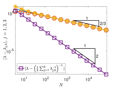
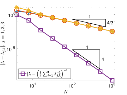
Figure 1: Regular example with $\mathbb{P}_{1}$, and $\mathbb{P}_{2}$ FEM in 1d.

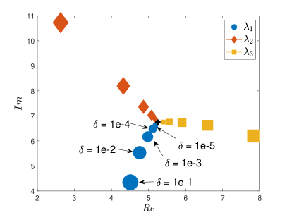
Figure 2: Sensitivity of eigenvalues due to $\delta$ perturbations of the real part of $c$.

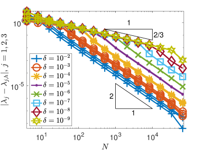
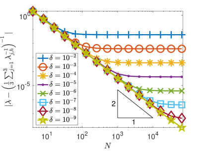
Figure 3: Convergence history for $\mathbb{P}_{1}$ FEM in 1d for $\delta$ perturbed problems with clustered eigenvalues.

In this example we align the jump of the diffusion coefficient with the mesh, so that the diffusion coefficient is piecewise constant on refined meshes. Although the continuous eigenfunctions are not globally smooth due to the jumping coefficient, they are piecewise smooth and if the mesh contains the jump point as a mesh point we can expect that the convergence orders are not reduced due to lower global regularity. In this light, we call this set of examples regular examples.

5.2 One-dimensional Example

Let $\Omega=(0,1)$ with $a=1$ on $[0,1/2]$ and $a=a_{\operatorname*{R}}$ on $(1/2,1]$, using the construction of the previous section, we compute

$$a_{\operatorname*{R}} =0.1069220800406739+0.08937533852238478i,$$

$$c =-0.9634059612381408+0.5989684988897067i,$$

for the first (smallest in magnitude) complex eigenvalue

$$\lambda=5.250721274740938+6.750931815875402i,$$

which has algebraic multiplicity $m_{alg}=3$ and ascent $\alpha=3$ by construction.

In Figure 1 we observe convergence rates according to the theory, in case of the $\mathbb{P}_{1}$ finite element method the convergence is of order $\mathcal{O}(N^{-2/3})$ (due to $\alpha=3$) for the eigenvalue errors $|\lambda-\lambda_{j,h}|$, $j=1,2,3$, and optimal convergence $\mathcal{O}(N^{-2})$ for the mean eigenvalue error. For the second order $\mathbb{P}_{2}$ finite element method we observe twice the convergence rate, i.e. $\mathcal{O}(N^{-4/3})$ for the eigenvalue errors, and $\mathcal{O}(N^{-4})$ for the mean eigenvalue error which show that the theoretical predicted rates are sharp for these examples.

Next, we investigate the sensitivity of the defective eigenvalue $\lambda$. Since the defect is very sensitive towards the choice of the parameters $a_{R}$ and $c$, we perturb only the real part of $c$ by adding a small (real) value $\delta$. In Figure 2, we observe that even very small perturbations $\delta$, immediately lead to a splitting of the defective eigenvalue into three clustered eigenvalues. Even a relatively small perturbation $\delta=10^{-2}$, of about 1%, already leads to a significant separation of the eigenvalues of size greater than $2$.

We investigate the transition of the defective eigenvalue into a separated cluster of eigenvalues in more detail and make the following observations in Figure 3. In the left figure we display the eigenvalue errors $|\lambda_{j}-\lambda_{j,h}|$, $j=1,2,3$, for $\mathbb{P}_{1}$ finite elements and different perturbations $\delta$ towards precomputed reference values $\lambda_{j}$ for the clustered eigenvalues. We computed the reference values with higher order $\mathbb{P}_{3}$ finite elements on fine meshes with high accuracy. In the right figure, we show the convergence of the mean eigenvalue error towards the defective eigenvalue $\lambda$. We observe that for $\delta=10^{-2}$ the eigenvalues are well separated, hence the three distinct eigenvalues converge with optimal rates and the mean eigenvalue error does not converge towards the defective eigenvalue $\lambda$. Interestingly, for smaller values of $\delta$, we observe that there seems to be a resolution barrier. Before a certain resolution is reached, we observe that the eigenvalue errors show the reduced convergence rate of approximating a defective eigenvalue, and even the mean value converges towards the defective eigenvalue $\lambda$. Once the mesh is fine enough, so that the clustered eigenvalues can be separated also on the discrete level, the eigenvalue errors converge with optimal rates and their mean value stops converging towards the defective eigenvalue.

In [13], other explicit choices of parameters are given such that the eigenvalue of the elliptic boundary value problem is defective.

5.3 Higher Dimensions

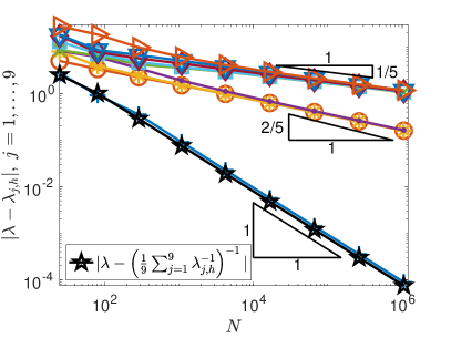
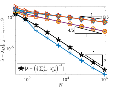
Figure 4: Regular example with $\mathbb{P}_{1}$, and $\mathbb{P}_{2}$ FEM in 2d.

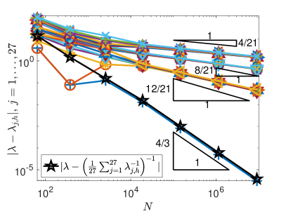
Figure 5: Regular example with $\mathbb{P}_{1}$, and $\mathbb{P}_{2}$ FEM in 3d.

We extend the one-dimensional example to higher dimensions $d=2,3$ by taking the tensor product of the (generalized) eigenfunctions in $x$, $y$ and $z$ coordinates, which leads to the eigenvalue $2\lambda$ in two dimensions of algebraic multiplicity $m_{alg}=9$, and the eigenvalue $3\lambda$ for $d=3$ with algebraic multiplicity $m_{alg}=27$. The diffusion coefficient and the boundary conditions are extended by tensorization to higher dimensions as well.

In two dimensions, we observe in Figure 4 for $\mathbb{P}_{1}$ finite elements convergence of at least $\mathcal{O}(N^{-1/5})$ for the eigenvalue errors and $\mathcal{O}(N^{-1})$ for the mean eigenvalue error. For $\mathbb{P}_{2}$ finite elements we observe twice the convergence, namely at least $\mathcal{O}(N^{-2/5})$ for the eigenvalue errors and $\mathcal{O}(N^{-2})$ for the mean eigenvalue error. This shows numerically the ascent $\alpha=5$. In addition, we observe that some discrete eigenvalues converge with rates in between those two extreme cases. Some eigenvalues converge with order close to $\mathcal{O}(N^{-2/5})$ for $\mathbb{P}_{1}$ finite elements and close to $\mathcal{O}(N^{-4/5})$ for $\mathbb{P}_{2}$ finite elements. Note that one eigenvalue seems to correspond to a discrete eigenvector, hence converges with the optimal rate.

For $d=3$, we observe in Figure 5 convergence rates of the eigenvalue errors as low as $\mathcal{O}(N^{-2/21})$ for $\mathbb{P}_{1}$ finite elements and $\mathcal{O}(N^{-4/21})$ for $\mathbb{P}_{2}$ finite elements, which indicate the ascent $\alpha=7$. Again the mean eigenvalue errors converge optimally. Note that some discrete eigenvalues converge with rates in between the optimal and reduced ones, and that one eigenvalue converges with optimal rate. In particular for $\mathbb{P}_{2}$ finite elements we observe that some eigenvalues converge with order $\mathcal{O}(N^{-8/21})$, and some even with order $\mathcal{O}(N^{-12/21})$, which relates to convergence order of $\mathcal{O}(h^{2k/7})$, for $k=2,3$. This confirms the impressive sharpness of the theory and that in principle any convergence order $\mathcal{O}(h^{pk/\alpha})$, for $k=1,\ldots,\alpha$, can occur, not only in theory, but as we have demonstrated also in practical computations.

5.4 Examples with Reduced Regularity

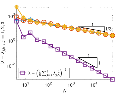
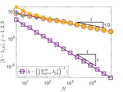
Figure 6: Example with reduced regularity for $\mathbb{P}_{1}$, and $\mathbb{P}_{2}$ FEM in 1d.

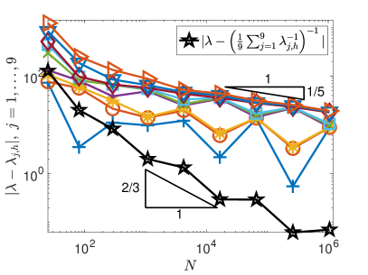
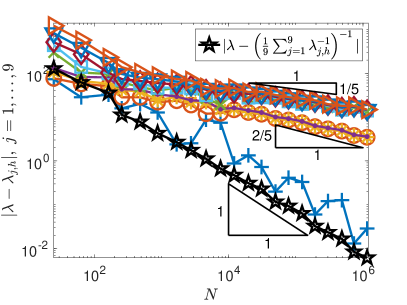
Figure 7: Example with reduced regularity for $\mathbb{P}_{1}$ FEM on uniform and adaptive meshes in 2d.

Here, we choose the coefficient $a$ such that its jump is not aligned with any (refined) mesh. Therefore, we consider $\Omega=(0,1)$ with $a=1$ on $[0,1/3]$ and $a=a_{\operatorname*{R}}$ on $(1/3,1]$, with

$$a_{\operatorname*{R}} =8.834634001449438+2.381273183203226i,$$

$$c =-23.62602259938114+23.10185194698031i,$$

and the first (smallest in magnitude) complex eigenvalue

$$\lambda=72.26224904068889+65.85698689932984i.$$

By construction $\lambda$ has algebraic multiplicity $m_{alg}=3$ and ascent $\alpha=3$ for $d=1$. As in the previous example, the tensor product of the (generalized) eigenfunctions leads to the eigenvalue $2\lambda$ with algebraic multiplicity $m_{alg}=9$ in two dimensions, and numerically we observe the ascent $\alpha=5$.

Note that since the mesh is not aligned with the jump of the diffusion coefficient, the regularity of the (generalized) eigenfunctions are reduced to $H^{1+r}\left(\Omega\right)$ for any $0<r<1/2$. Therefore, we observe reduced convergence of the eigenvalues due to the reduced convergence of the (generalized) eigenfunctions on uniform meshes.

In Figure 6, we see that the convergence is reduced by two separate issues: the reduced regularity and the large defect of the eigenvalue. We observe the theoretically expected suboptimal convergence rates of the mean eigenvalue error of $\mathcal{O}(N^{-1})$ for both $\mathbb{P}_{1}$ and $\mathbb{P}_{2}$ finite elements due to the reduced regularity. The convergence of the eigenvalue errors is even further reduced due to the defect $\alpha=3$, hence the convergence is only of order $\mathcal{O}(N^{-1/3})$.

The situation in two dimensions is less clear from the numerical point of view. In Figure 7, we observe in the left figure reduced rates of the mean eigenvalue error for $\mathbb{P}_{1}$ finite elements on uniform meshes, but still at worst $\mathcal{O}(N^{-1/5})$ convergence of the eigenvalues, which is expected from the defect of $\lambda$, but is not further decreased by the low regularity. This might be a pre-asymptotic effect. In the right figure we use an adaptive mesh refinement algorithm [14, 15, 19, 29]. Based on the previous observation, that even very small perturbations lead to a split of the defective eigenvalue into clustered eigenvalues, we measure the error of the defective eigenvalue, as if it was a cluster of eigenvalues, with the a posteriori error estimator

$$\eta_{h}^{2} :=\sum_{j=1}^{m}\sum_{T\in\mathcal{T}}\big{(}h_{T}^{2}\|\Delta u_{j,h}+\lambda_{j,h}u_{j,h}\|_{0,T}^{2}+\sum_{E\subset\partial T\backslash\partial\Omega}h_{E}\|[a\nabla u_{j,h}\cdot\mathbf{n}]\|_{0,E}^{2}$$

$$\quad+\sum_{E\subset\partial T\cap\Gamma_{\operatorname*{R}}}h_{E}\|a\nabla u_{j,h}\cdot\mathbf{n}+cu_{j,h}\|_{0,E}^{2}$$

$$\quad+h_{T}^{2}\|\Delta u_{j,h}^{*}+\lambda_{j,h}^{*}u_{j,h}^{*}\|_{0,T}^{2}+\sum_{E\subset\partial T\backslash\partial\Omega}h_{E}\|[\overline{a}\nabla u_{j,h}^{*}\cdot\mathbf{n}]\|_{0,E}^{2}$$

$$\quad+\sum_{E\subset\partial T\cap\Gamma_{\operatorname*{R}}}h_{E}\|\overline{a}\nabla u_{j,h}^{*}\cdot\mathbf{n}+\overline{c}u_{j,h}^{*}\|_{0,E}^{2}\big{)},$$

where $(\lambda_{j,h}^{*},u_{j,h}^{*})$ denotes the $j$-th eigenpair of the adjoint eigenvalue problem. Despite that $\eta_{h}^{2}$ provides only a valid upper bound for clustered eigenvalues, we observe in Figure 7 that adaptive mesh-refinement based on $\eta_{h}^{2}$ leads to optimal convergence of the mean eigenvalue error. By construction, $\eta_{h}^{2}$ cannot give any a posteriori information about the ascent of the eigenvalue. Nevertheless, this experiment illustrates that an error estimator is in principle able to heuristically detect defective eigenvalues from their reduced convergence rates, although a theoretical foundation has still to be developed.

6 Conclusions

We described a constructive way of deriving benchmark problems with highly defective eigenvalues. We provided the parameters for two such examples. We confirmed in numerical experiments that the Babuška-Osborn theory is sharp and that convergence rates between the two extreme cases do occur in practical computations. Since even for non-smooth eigenfunctions, the mean eigenvalue error converges faster, one is in principle able to detect defective eigenvalues numerically by tracking the convergence behavior of the eigenvalues and the mean eigenvalue error on uniformly or adaptively refined meshes. If the mean eigenvalue error converges faster, that means that the eigenvalue is defective.

References

• [1] I. Babuška and J. Osborn. Eigenvalue problems. In Handbook of numerical analysis, Vol. II, Handb. Numer. Anal., II, pages 641–787. North-Holland, Amsterdam, 1991.
• [2] S. C. Brenner and L. R. Scott. The mathematical theory of finite element methods, volume 15. Springer, New York, third edition, 2008.
• [3] C. Carstensen, J. Gedicke, V. Mehrmann, and A. Miedlar. An adaptive homotopy approach for non-selfadjoint eigenvalue problems. Numer. Math., 119:557–583, 2011
• [4] F. Chatelin. La méthode de Galerkin. Ordre de convergence des éléments propres. C.R. Acad. Sci. Pairs Sér. A, 278:1213–1215, 1974.
• [5] F. Chatelin. Spectral Approximation of Linear Operators. Academic Press, New York, 1983.
• [6] P. Ciarlet. The finite element method for elliptic problems. North-Holland, 1987.
• [7] R. Dautray and J.-L. Lions. Mathematical analysis and numerical methods for science and technology. Vol. 3. Springer-Verlag, Berlin, 1990. Spectral theory and applications, With the collaboration of Michel Artola and Michel Cessenat, Translated from the French by John C. Amson.
• [8] J. W. Demmel. Applied numerical linear algebra. Society for Industrial and Applied Mathematics (SIAM), Philadelphia, PA, 1997.
• [9] N. Dunford and J. Schwartz. Linear Operators Part II: Spectral Theory. Wiley-Interscience, New York, New York, 1963.
• [10] E. Dyakonov. Optimization in solving elliptic problems. CRC Press, Boca Raton, 1996.
• [11] D. J. Ewins. Modal testing: theory and practice, volume 15. Research studies press Letchworth, 1984.
• [12] B. Friedman. Principles and techniques of applied mathematics. John Wiley & Sons, Inc., New York; Chapman & Hall, Ltd., London, 1956.
• [13] R. Gasser. The Finite Element Method for Elliptic Problems with Defective Eigenvalues. Master’s thesis, Inst. f. Mathematik, Unversität Zürich, 2017. http://www.math.uzh.ch/compmath/index.php?id=dipl.
• [14] J. Gedicke and C. Carstensen. A posteriori error estimators for convection-diffusion eigenvalue problems. Comput. Methods Appl. Mech. Engrg., 268:160–177, 2014.
• [15] S. Giani, L. Grubišić, A. Miedlar, and J. S. Ovall. Robust error estimates for approximations of non-selfadjoint eigenvalue problems. Numer. Math., 133(3):471–495, 2016.
• [16] P. Grisvard. Elliptic Problems in Nonsmooth Domains. Pitman, Boston, 1985.
• [17] W. Hackbusch. Elliptic Differential Equations. Springer Verlag, Berlin, 1992.
• [18] Z.-F. Fu and J. He. Modal analysis. Elsevier, 2001.
• [19] V. Heuveline and R. Rannacher. A posteriori error control for finite approximations of elliptic eigenvalue problems. Adv. Comput. Math., 15(1-4):107–138 (2002), 2001.
• [20] J. Jackson. Classical Electrodynamics. John Wiley & Sons, New York, NY, 3 edition, 1998.
• [21] T. Kato. Perturbation theory for linear operators. Springer-Verlag, Berlin, 1966.
• [22] A. Knyazev. Sharp a priori error estimates of the Raleigh-Ritz method without assumptions of fixed sign or compactness. Mathematical Notes, 38(5-6):998–1002, 1986.
• [23] A. Knyazev and J. Osborn. New a priori FEM error estimates for eigenvalues. SIAM J. Numer. Anal., 48(6):2647–2667, 2006.
• [24] M. Machover. The alternative theorem and the nonselfadjoint generalized Green’s function. J. Differential Equations, 35(2):266–274, 1980.
• [25] H. G. Natke. Einführung in Theorie und Praxis der Zeitreihen-und Modalanalyse: Identifikation schwingungsfähiger elastomechanischer Systeme. Springer-Verlag, 2013.
• [26] E. Ovtchinnikov. Cluster robust error estimates for the Raleigh-Ritz approximation I: Estimates for invariant subspaces. LAA, 415(1):167–187, 2006.
• [27] S. Sauter. $hp$-finite elements for elliptic eigenvalue problems: error estimates which are explicit with respect to $\lambda$, $h$, and $p$. SIAM J. Numer. Anal., 48(1):95–108, 2010.
• [28] G. Strang and G. Fix. An Analysis of the Finite Element Method. Prentice-Hall, Englewood Cliffs, 1973.
• [29] Y. Yang, L. Sun, H. Bi, and H. Li. A note on the residual type a posteriori error estimates for finite element eigenpairs of nonsymmetric elliptic eigenvalue problems. Appl. Numer. Math., 82:51–67, 2014.