Ocean Dynamics and the Inner Edge of the Habitable Zone for Tidally Locked Terrestrial Planets

Abstract

Recent studies have shown that ocean dynamics can have a significant warming effect on the permanent night sides of 1:1 tidally locked terrestrial exoplanets with Earth-like atmospheres and oceans in the middle of the habitable zone. However, the impact of ocean dynamics on the habitable zone’s boundaries (inner edge and outer edge) is still unknown and represents a major gap in our understanding of this type of planets. Here we use a coupled atmosphere-ocean global climate model to show that planetary heat transport from the day to night side is dominated by the ocean at lower stellar fluxes and by the atmosphere near the inner edge of the habitable zone. This decrease in oceanic heat transport (OHT) at high stellar fluxes is mainly due to weakening of surface wind stress and a decrease in surface shortwave energy deposition. We further show that ocean dynamics have almost no effect on the observational thermal phase curves of planets near the inner edge of the habitable zone. For planets in the habitable zone’s middle range, ocean dynamics moves the hottest spot on the surface eastward from the substellar point. These results suggest that future studies of the inner edge may devote computational resources to atmosphere-only processes such as clouds and radiation. For studies of the middle range and outer edge of the habitable zone, however, fully coupled ocean-atmosphere modeling will be necessary. Note that due to computational resource limitations, only one rotation period (60 Earth days) has been systematically examined in this study; future work varying rotation period as well as other parameters such as atmospheric mass and composition is required.

1 Introduction

The ocean has a profound effect on the variation and time-mean features of the climate of Earth through modifying the surface heat capacity, transporting heat from low latitudes to high latitudes and storing carbon (Vallis, 2012; Watson et al., 2015). The tight interaction between ocean, atmosphere, ice and clouds further influence global and regional energy balances and surface temperatures. For instance, if Earth’s global ocean circulation were artificially turned off, the global-mean surface temperature would decrease by several degrees (Winton, 2003; Herweijer et al., 2005). How ocean dynamics influence the climate and habitability of exoplanets remains relatively unstudied.

During the past 20 years, various three-dimensional (3D) atmosphere-only climate models have been employed to examine the important effects of atmospheric circulation on the climate and habitability of 1:1 tidally locked (‘synchronously rotating’) terrestrial planets (e.g., Joshi et al., 1997; Merlis & Schneider, 2010; Edson et al., 2011; Pierrehumbert, 2011; Leconte et al., 2013a, b; Yang et al., 2013, 2014; Wang et al., 2014, 2016; Way et al., 2015; Kopparapu et al., 2016; Popp et al., 2016; Turbet et al., 2016; Salameh et al., 2017; Wolf, 2017; Wolf et al., 2017; Haqq-Misra et al., 2017; Boutle et al., 2017; Kopparapu et al., 2017; Bin et al., 2018; Turbet et al., 2018). These studies employed a dry land surface with no ocean or an immobile thermodynamic ocean with no ocean dynamics. The effect of ocean dynamics on exoplanets has only been addressed by a few studies (Yang et al., 2013, 2014; Hu & Yang, 2014; Cullum et al., 2014, 2016; Way et al., 2015, 2018; Del Genio et al., 2019). Studies on synchronously rotating planets have found that ocean dynamics could significantly warm the permanent night sides of planets in the middle range of the habitable zone (Hu & Yang (2014) and Del Genio et al. (2019), or see section 3.1 for more detailed feedback analyses). A critical unaddressed question is: Could ocean dynamics have a significant effect on the location of the inner edge of the habitable zone? If ocean dynamics have a strong warming effect on planets near the inner edge, as they do for those in the middle range, this could shrink the habitable zone. As a result, the number of potentially habitable planets would be lower, making it harder to detect and study such planets in the future. Here we try to answer this question through a series of 3D climate experiments.

The maximum stellar flux investigated by Hu & Yang (2014), 1,400 W m^-2, is only about 40-50 % of the stellar flux at the inner edge, according to results from atmosphere-only models (Yang et al., 2014; Kopparapu et al., 2017; Bin et al., 2018). Our new experiments show that the day-to-night oceanic heat transport (OHT) at the higher stellar fluxes of planets near the inner edge is much weaker than that for a stellar flux of 1,400 W m^-2 (see section 3.2) and that the location of the inner edge would not be shifted by ocean dynamics, at least for a rotation period of 60 Earth days. Section 2 addresses the model description and experimental design. We show the results in section 3, including the effect of ocean dynamics on planets in the middle range (section 3.1) and near the inner edge (section 3.2) of the habitable zone, the effect of ocean dynamics on observational thermal phase curves (section 3.3) and an exception to our result that OHT tends to monotonically decrease with increasing stellar flux (section 3.4). We further discuss the results and suggest future required studies in section 4, and summarize in section 5.

2 Model Description and Experimental Design

We use the Community Climate System Model CCSM3, which has four coupled components: atmosphere, ocean, land and sea ice (Collins et al., 2006). The model was developed to investigate the climates of present, past and future Earth. We have modified the model to be able to simulate the climates of Earth-like exoplanets that have different stellar spectra, planetary orbits, masses, and land-sea distributions (Liu et al., 2013; Hu & Yang, 2014; Yang et al., 2014). By default, we use a planetary surface nearly completely covered with an ocean of water (“an aqua-planet”) with a uniform depth of $\simeq$ 4,000 m, close to the mean depth of Earth’s oceans. We include two small islands at the south and north poles (poleward of 85 ^∘S(N)) because the poles of the ocean grid have to reside on continents (Rosenbloom et al., 2011). These small-area islands should have a negligible influence on the results. Aqua-planet simulations provide a standard framework for understanding large-scale ocean circulations and for relating our results to previous work, including analytical theories (Smith et al., 2006; Marshall et al., 2007). Also, due to the lack of complex land barriers, an aqua-planet represents the simplest fully 3D and coupled system in which to investigate ocean circulation and ocean-atmosphere interaction, and therefore is most appropriate for examining the mechanisms that strengthen or weaken the ocean’s effect at different stellar fluxes.

The atmosphere is assumed to be Earth-like, composed of N₂ and H₂O, with a surface pressure of approximately 1.0 bar (depending on the water vapor concentration). The concentrations of CO₂, CH₄, N₂O, O₂, O₃ and CFCs are set to zero. Water vapor is the only greenhouse gas. We chose one sample star with a surface temperature of 4,500 K. The rotation period of the planet is 60 Earth days ($=$ orbital period), and the stellar fluxes we tested are 1,400, 1,600, 1,800, 2,000, 2,200, 2,400, 2,600, and 2,800 W m^-2. The maximum stellar flux for which the model can achieve a quasi-equilibrium state is 2,800 W m^-2. The radius and gravity of the simulated planet are set to typical values of a super-Earth (such as the unconfirmed exoplanet Gl 581g (Vogt et al., 2010) and the confirmed exoplanet LHS 1140b (Dittmann et al., 2017)): 1.5 times Earth’s radius and 1.38 times Earth’s gravity. Both obliquity and eccentricity are set to zero.

Table 1: Summary of the climate simulations performed using CCSM3

Group	Runs	Experimental Design
Control	1	The surface is covered by an ocean with a uniform depth of about 4,000 m. The stellar flux is 1,400 W m-2 with a 4,500-K blackbody spectrum. Rotation period ($=$ orbital period) is 60 Earth days.
Stellar flux	9	Same as ‘Control’ except the stellar flux is varied between 1,400 and 2,800 W m-2 in increments of 200 W m-2.
Initial state	2	Same as ‘Control’ except stellar flux is set to 1,800 W m-2 and the initial state is from the equilibrium state of the case of 2,400 W m-2, or the stellar flux is set to 2,400 W m-2 and the initial state is from the equilibrium state of the case of 1,800 W m-2.
Ocean depth	3	The ocean depth is set to 4,000, 800 and 400 m, respectively. The stellar flux is 1,400 W m-2 with a 3,400-K blackbody spectrum. Rotation period ($=$ orbital period) is 37 Earth days.
Land-sea distribution	2	One-ridge world: a thin barrier that completely obstructs ocean flows running from pole to pole on the eastern terminator. Two-ridges world: two thin barriers on the western and eastern terminators. Other parameters are the same as the ‘Ocean depth’ cases.

In our simulations, for a given stellar temperature, the rotation period is fixed when varying the stellar flux, as was done by Wang et al. (2014), Way et al. (2015), and Fujii et al. (2017). The period of 60 Earth days we chose is close to the rotation period near the inner edge of the habitable zone for a star with a temperature of 4,500 K (see Fig. 2 of ref. Kopparapu et al. (2016)). This design allows us to isolate the effect of increasing stellar radiation and is sufficient to demonstrate the role of ocean dynamics on the inner edge of the habitable zone. Our setup is different from that employed by Kopparapu et al. (2016), Haqq-Misra et al. (2017) and Wolf et al. (2017), who modified the rotation period and stellar flux simultaneously. Their experiments are able to self-consistently consider the combined effect of the Coriolis force and stellar flux, but do not allow the separate consideration of each factor. In the future, it would be interesting to investigate the combined effect of varying the rotation period and stellar flux using a coupled atmosphere–ocean model.

In order to test the effect of continent and ocean depth on the ocean circulation, we also carried out experiments with a one-ridge or a two-ridges continental setup or different ocean depths, 800 and 400 m (Table 1). The geothermal heat flux is set to zero, and the only energy source is stellar radiation. We find our results are robust across these parameters but future work is required to consider whether our results are strongly sensitive to additional effects, such as other resonant orbital-rotational states, different planetary radii and gravities, different land-sea distributions, and other ocean depths.

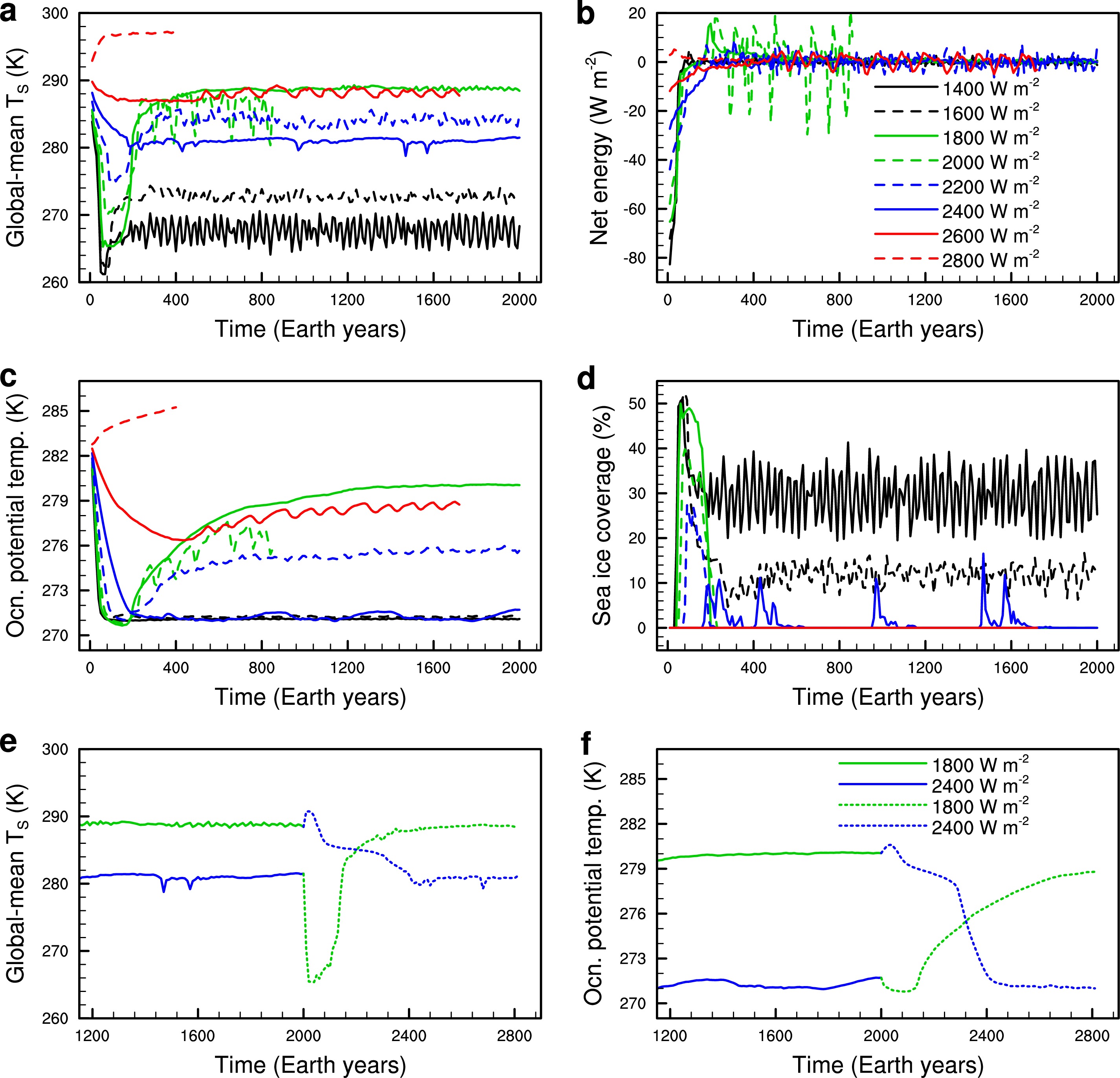
Figure 1: Time series of global-mean characteristics of the CCSM3 simulations. (a), surface air temperature; (b), net energy flux (shortwave minus longwave) at the top of the atmosphere; (c), vertically-averaged ocean potential temperature; and (d), sea ice coverage. The stellar flux is increased from 1,400 to 2,800 W m^-2 in increments of 200 W m^-2. (e-f), independence of the equilibrium state from the initial state, for the stellar fluxes of 1,800 and 2,400 W m^-2. (e), global-mean surface temperature; and (f), global- and vertical-mean ocean potential temperature. In (e-f), the solid lines are the same as those shown in (a) and (c), and the dotted lines are initialized from the equilibrium states of the solid lines. Each data point in these time series is the average over 10 Earth years. In all of these experiments, the rotation period is 60 Earth days and we apply a 4,500-K blackbody spectrum and an aqua-planet with a uniform depth of $\simeq$ 4000 m.

In the ocean component of our model, diffusion and viscosity parameters are assumed to be the same as for Earth’s present-day oceans. The parameterization of along-isopycnal potential temperature and salinity diffusion uses the Gent-McWilliams scheme (Gent & McWilliams, 1990) with a coefficient of 800 m² s^-1. Horizontal viscosity in the momentum equation employs the anisotropic formulation (Smith & McWilliams, 2003). Diapycnal mixing is represented by the K-profile parameterization boundary-layer scheme (Large et al., 1990). Several physical processes are considered in the scheme, including internal waves, shear instability, convective instability and double diffusion (Smith & Gent, 2004). Separate studies using high-resolution eddy-resolving ocean models are required to understand the uncertainties of these parameters for Earth-like exoplanets; computational resource limitations preclude such sensitivity experiments at present.

The atmosphere and land components of the model have a horizontal resolution of 3.75^∘ $\times$ 3.75^∘ and with 26 vertical levels from the surface to $\sim$36 km. The ocean and sea-ice components have a variable latitudinal resolution starting at 0.9^∘ near the equator, a constant longitudinal resolution of 3.6^∘, and 25 vertical levels. By default, the time step for the atmosphere and land components is set to 900 s. For the simulations with high stellar fluxes, we used a smaller time step to avoid numerical instability; the minimum time step we examined is 60 s. Due to computational limitations, time steps less than 60 s were not tested. For the ocean, the time step is two hours. The coupling time interval between the atmosphere and ocean is one Earth day. The sea ice albedo is 0.50 in the visible and 0.30 in the near infrared. The snow albedo is 0.91 in the visible and 0.63 in the near infrared (Briegleb et al., 2002). The broadband surface albedo, therefore, depends on stellar spectrum and is less reflective at redder wavelengths (Joshi & Haberle, 2012; Shields et al., 2013).

The atmosphere was initialized from a state close to modern Earth, and the ocean was initialized from a state of rest with a horizontally uniform temperature. We integrated each case for about 1,000 or 2,000 Earth years, and present the final 100 or 200 years in the following analyses. Time series of global-mean surface temperature, energy balance (absorbed shortwave radiation minus outgoing longwave radiation) at the top of the atmosphere, vertically averaged ocean potential temperature, and sea ice coverage are shown in Fig. 1(a-d). In most cases, the system reaches quasi-equilibrium within about 1,000 years, although several simulations exhibit significant oscillations after that time: (1) The 2,000 and 2,600 W m^-2 cases show strong oscillations with a period of $\simeq$ 100 Earth years; (2) the 1,400 and 1,600 W m^-2 cases also exhibit significant variations but with a period of $\simeq$ 30 Earth years; (3) the 2,400 W m^-2 case shows irregular risings in sea ice coverage and fallings in sea temperature and ocean potential temperature. We speculate that these long-time oscillations may arise from the interactions between atmosphere, sea ice and ocean (especially Rossby and Kelvin waves), such as that shown in Marshall et al. (2007); detailed analyses of the underlying mechanisms are beyond the scope of the present work. In this paper, we will focus on the mean state only. Note that ocean potential temperature in the 2,800 W m^-2 case is still increasing although the surface temperature does not show a significant warming trend; the model blew up when we tried to further integrate the run. If the model could be integrated longer, the ocean would become warmer especially in relatively cold regions at the ocean bottom and the ocean in the night side, so that OHT from the day side to the night side (see section 3.2 below) would likely be even smaller.

In the following section, we will analyze our equilibrated CCSM3 simulations to understand the ocean’s effect on the planetary climates. To isolate the effect of ocean dynamics, we preformed corresponding atmosphere-only experiments using the Community Atmosphere Model version 3.1 (CAM3, Collins et al. (2004)), which is the atmosphere component of CCSM3. CAM3 is coupled with a 50-m mixed layer, immobile ocean, and ocean heat transport is specified to be zero everywhere. The model is coupled to a thermodynamic sea ice model, in which sea ice flows are not considered. Each case is integrated for about 60 Earth years and reaches a steady state after about 40 years. Averages over the last 5 years are used for our analyses. The maximum stellar flux for which simulations in CAM3 can achieve a quasi-equilibrium state is 3,000 W m^-2, higher than that in CCSM3.

3 Results

3.1 The Ocean’s strong effect in the middle of the habitable zone

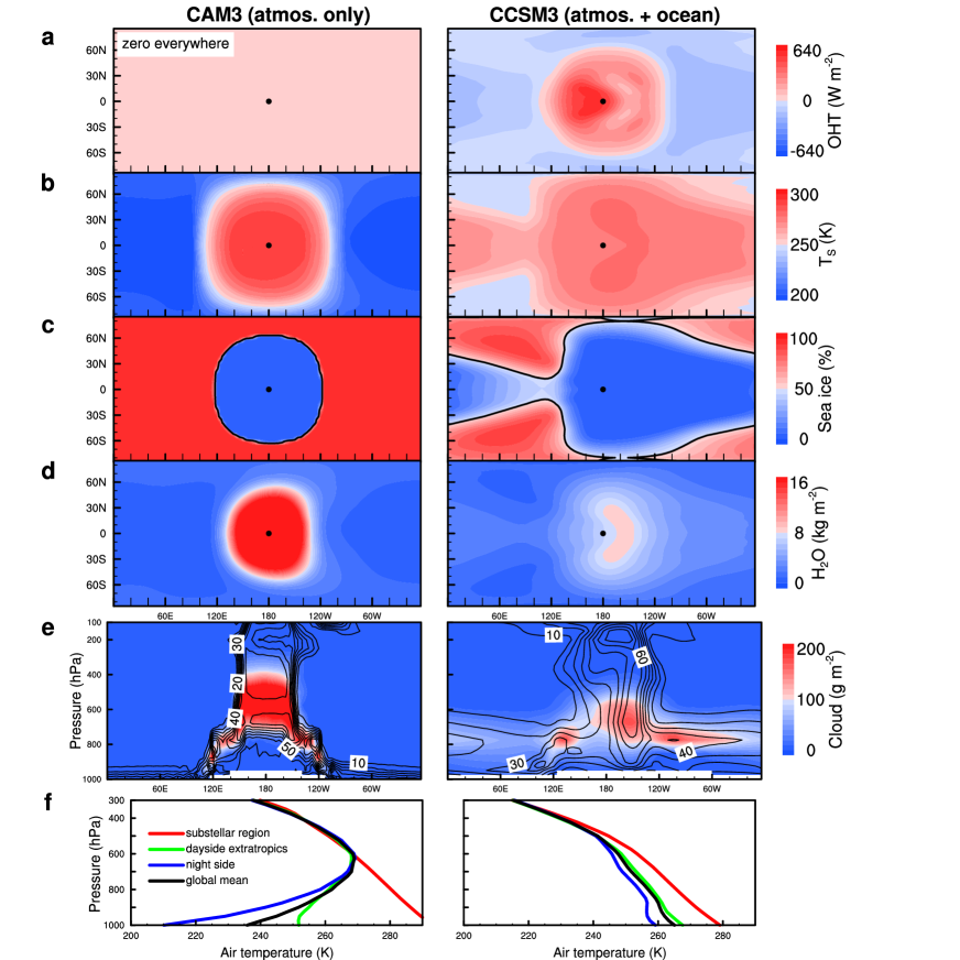
Figure 2: Strong effects of ocean dynamics on a tidally locked aqua-planet in the middle range of the habitable zone. Left: CAM3, and right: CCSM3. (a), OHT (i.e., surface net heat flux; negative: heat from ocean to atmosphere, positive: heat from atmosphere to ocean); (b), surface temperature; (c), sea ice coverage (the black line shows 50 % coverage); (d), vertically integrated water vapor amount; (e), meridional-mean cloud water amount (color shading) and cloud fraction (%, contour lines with an interval of 10 %); and (f), vertical temperature profiles for different regions. Note the vertical axis is latitude in (a-d) but air pressure in (e-f). In both experiments, the stellar flux is 1,400 W m^-2. In this figure and elsewhere, the substellar point is at (180^∘, 0^∘) and is marked with a black dot.

The ocean transports heat from the substellar region where there is net energy gain to the night side where there is net energy loss. As a result, the night side in CCSM3 is much warmer than that in CAM3 by 40-50 K (Fig. 2; see also Hu & Yang (2014) and Del Genio et al. (2019)). The ocean also transports heat in the north-south direction and thereby warms the dayside high latitudes. Despite the ocean transporting heat away from the substellar region, surface temperatures there decrease only slightly, by $\simeq$ 10 K. This is mainly due to a negative cloud feedback: As the OHT carries energy away from the substellar region, the surface temperature decreases and therefore convection over the substellar region becomes weaker, so that cloud optical depth (Fig. 2(e)) and planetary albedo decrease, allowing more stellar energy to reach the surface and warm it. This feedback is similar to that described in Koll & Abbot (2013). Moreover, per unit of energy, the warming of the nightside surface should be greater than the cooling of the dayside surface because of the nonlinear dependence of thermal emission on temperature (i.e., the Planck effect) and the fact that the nightside surface is colder than the dayside surface.

Besides the direct effect of ocean dynamics, feedbacks associated with sea ice, water vapor and atmospheric lapse rate further act to warm the surface. OHT melts the sea ice around the terminators and at the dayside high latitudes (Fig. 2(c)), reducing the planetary albedo. Meanwhile, in the experiments with stellar fluxes equal to or less than 1,600 W m^-2, sea ice in CCSM3 is only several meters thick, being 2-3 orders of magnitude thinner than the nightside sea ice thickness in CAM3, similar to the results in Yang et al. (2014), so OHT is effective at preventing water trapping on the night side. For stellar fluxes higher than 1,600 W m^-2, there is no snow or ice either on the day or night side in CCSM3, although in CAM3 the night side is still covered by ice and snow. Compared to CAM3, CCSM3’s water vapor concentration is higher on the night side (Fig. 2(d), although lower in the substellar region), the temperature inversion (i.e., air temperature being higher than the surface, ref. Zalucha et al. (2013); Leconte et al. (2013b); Yang & Abbot (2014a)) disappears on the night side (Fig. 2(f)), and the longwave cloud radiative effect is higher (a warming effect, Fig. 3). All of these factors act to increase the atmospheric greenhouse effect on the night side in CCSM3. In contrast, on the night side in CAM3, clouds form at the layers near the temperature inversion (Fig. 2(f)), which acts to trap water vapor that evaporated from the surface; this mechanism is similar to the low-level stratus cloud formation over the eastern subtropical Pacific Ocean where the sea surface is cooler than average sea surface due to ocean upwelling there (ref. Chapter 3.13 of Hartmann (2016)). These clouds emit longwave radiation to space at temperatures higher than the surface, causing a negative longwave cloud radiative effect on the night side (Fig. 3(b)) and inducing a cooling effect on the air and the surface, except the case of 3,000 W m^-2 in which the temperature inversion disappears. In CCSM3, there is no temperature inversion in all of the experiments shown here (note that for a much lower stellar flux, such as 625 W m^-2 in which ocean heat transport is very weak, there is a temperature inversion (figure not shown)) and the longwave cloud radiative effect is positive (warming) everywhere.

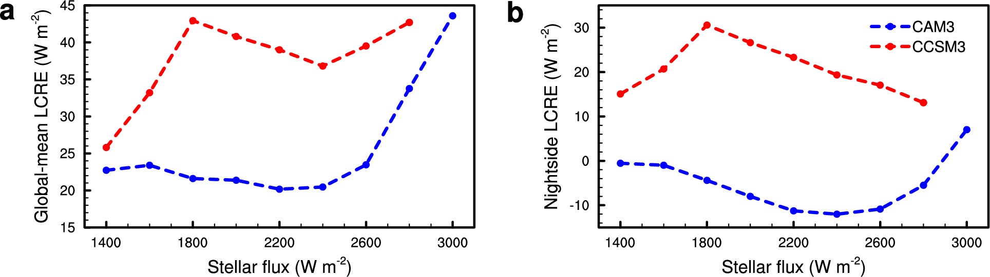
Figure 3: Longwave cloud radiative effect (LCRE) at the top of the atmosphere. Blue: CAM3, and red: CCSM3. (a), global mean, and (b), nightside average.

The direct effect of ocean dynamics is therefore to reduce the day-to-night surface temperature contrast in CCSM3 compared to CAM3. Associated surface and atmospheric feedbacks then amplify the nightside warming, which is why global-mean surface temperature in CCSM3 is much higher than that in CAM3 (Fig. 2(b)). However, as we show in the next section, these differences become smaller and smaller as the stellar flux is increased.

3.2 Decreasing Trend of OHT With Increasing Stellar Flux

As the stellar flux is increased, the global-mean surface temperature (as well as the maximum and minimum surface temperatures) in CCSM3 generally increases, but the area-averaged day-to-night OHT decreases when the stellar flux is higher than 1,800 W m^-2 (Fig. 4, for a discussion of the non-monotonic behavior of CCSM3’s results, see section 3.4). This finding seems counterintuitive because as the energy received by the day side of the planet increases, one might expect the ocean to transport more heat to the night side. This intuition does hold for the atmospheric and total (oceanic plus atmospheric) heat transports, which do increase with stellar flux (Fig. 4(b)), but not for the OHT.

Fig. 4(b) indicates that there is a compensation between OHT and atmospheric heat transport, but the compensation is imperfect. In CAM3, the OHT is zero and the atmospheric heat transport is higher than that in CCSM3. The total heat transport, however, is higher in CCSM3 than that in CAM3. The main reason is that the planetary albedo in CCSM3 is smaller (Fig. 4(i)), meaning that more stellar radiation is absorbed by the dayside atmosphere and surface; therefore more energy can be supplied to transport by the atmosphere and ocean. This result is consistent with previous results (Vallis & Farneti, 2009; Enderton & Vallis, 2009; Farneti & Vallis, 2013): Increased atmospheric heat transport generally picks up the slack of reduced OHT, but the compensation is often not 100 %.

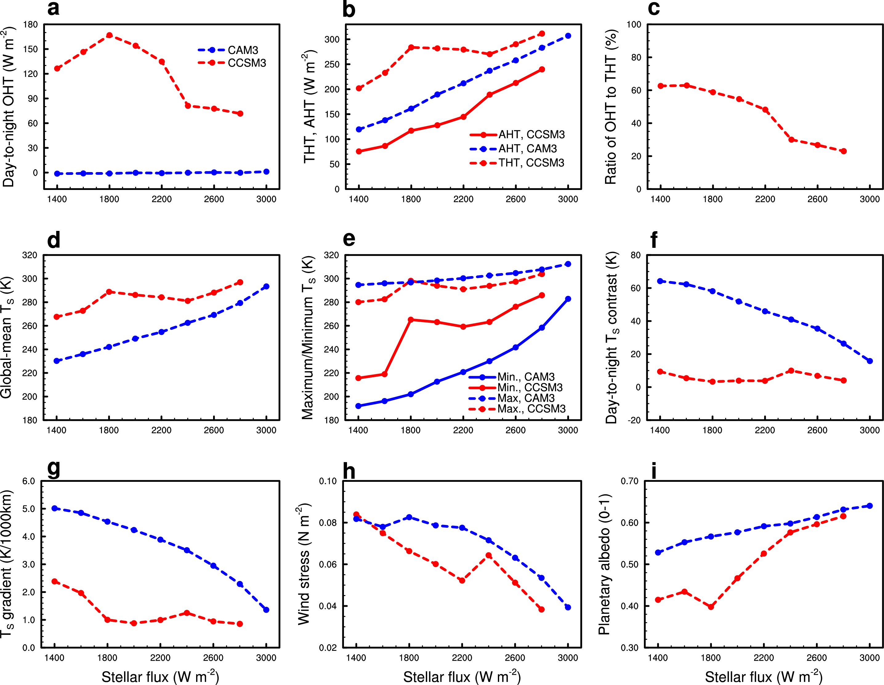
Figure 4: The effect of ocean dynamics as a function of stellar flux. Blue line: the atmosphere-only model CAM3, and red line: the coupled ocean-atmosphere model CCSM3. (a), area-averaged day-to-night oceanic heat transport (OHT); (b), day-to-night atmospheric heat transport (AHT) and total heat transport (THT); (c), the ratio of OHT to THT in CCSM3; (d), global-mean surface temperature (T_S); (e) maximum surface temperature (dashed line) and minimum surface temperature (solid line); (f) day-to-night area-averaged T_S contrast; (g) strength of surface temperature gradient ($\sqrt{(\frac{\partial T_{S}}{\partial x})^{2}+(\frac{\partial T_{S}}{\partial y})^{2}}$ in units of K per 1,000 km); (h) strength of surface wind stress ($\sqrt{\tau_{x}^{2}+\tau_{y}^{2}}$ where $\tau_{x}$ is the zonal wind stress and $\tau_{y}$ is the meridional wind stress); and (i) planetary albedo, as a function of stellar flux. In all of the experiments, the rotation period is 60 Earth days and the stellar spectrum is a 4,500-K blackbody.

The decreasing trend of OHT with increasing stellar flux results from weaker ocean currents combined with less stellar radiation depositing energy at the dayside sea surface. The main characteristic of ocean circulation on a tidally locked aqua-planet is west-east currents along the equator (Fig. 5(i-p), ref. Hu & Yang (2014)). The ocean currents in the tropics result from the combined effect of surface wind stresses and equatorward momentum transport by large-scale Rossby and Kelvin waves in the ocean (more comprehensive analyses and detailed dynamical diagnostics will be addressed in a separate paper, Yaoxuan Zeng, Yonggang Liu, & Jun Yang: Understanding the wind-driven ocean circulation on a tidally locked aqua-planet, manuscript in preparation, 2018). Surface temperature gradients on the east side of the substellar point are smaller than those on its west side (see the right panel of Fig. 2(b)). Due to this asymmetry, the eastward stresses on the west side of the substellar point are generally stronger than the westward stresses on the east side of the substellar point (Fig. 5(a-h)), so the net effect of the surface stresses is to drive eastward ocean flows. As the stellar flux is increased, the ocean flows become weaker (Fig. 5(i-p)) due to weaker surface wind stresses (Figs. 4(h) and 5(a-h)). The decrease in surface wind stresses at least partly results from a smaller surface temperature gradient (Fig. 4(g)), which is associated with the greater warming of the night side compared to the day side.

The ocean currents become ineffective when the stellar flux is equal to 2,400 W m^-2 or higher (Fig. 5(n-p)). Our result of small horizontal temperature gradients and weak surface wind stresses when the stellar flux is high is compatible with previous work on hot climates under high levels of insolation or atmospheric CO₂. Examples of this are shown in Fig. 1 of Leconte et al. (2013a) for the climate simulation of Earth under a brightening sun, in Fig. 2 of Way et al. (2016) for a temperate Venus, and in Fig. 4 of Wolf (2017) for the exoplanet TRAPPIST 1d.

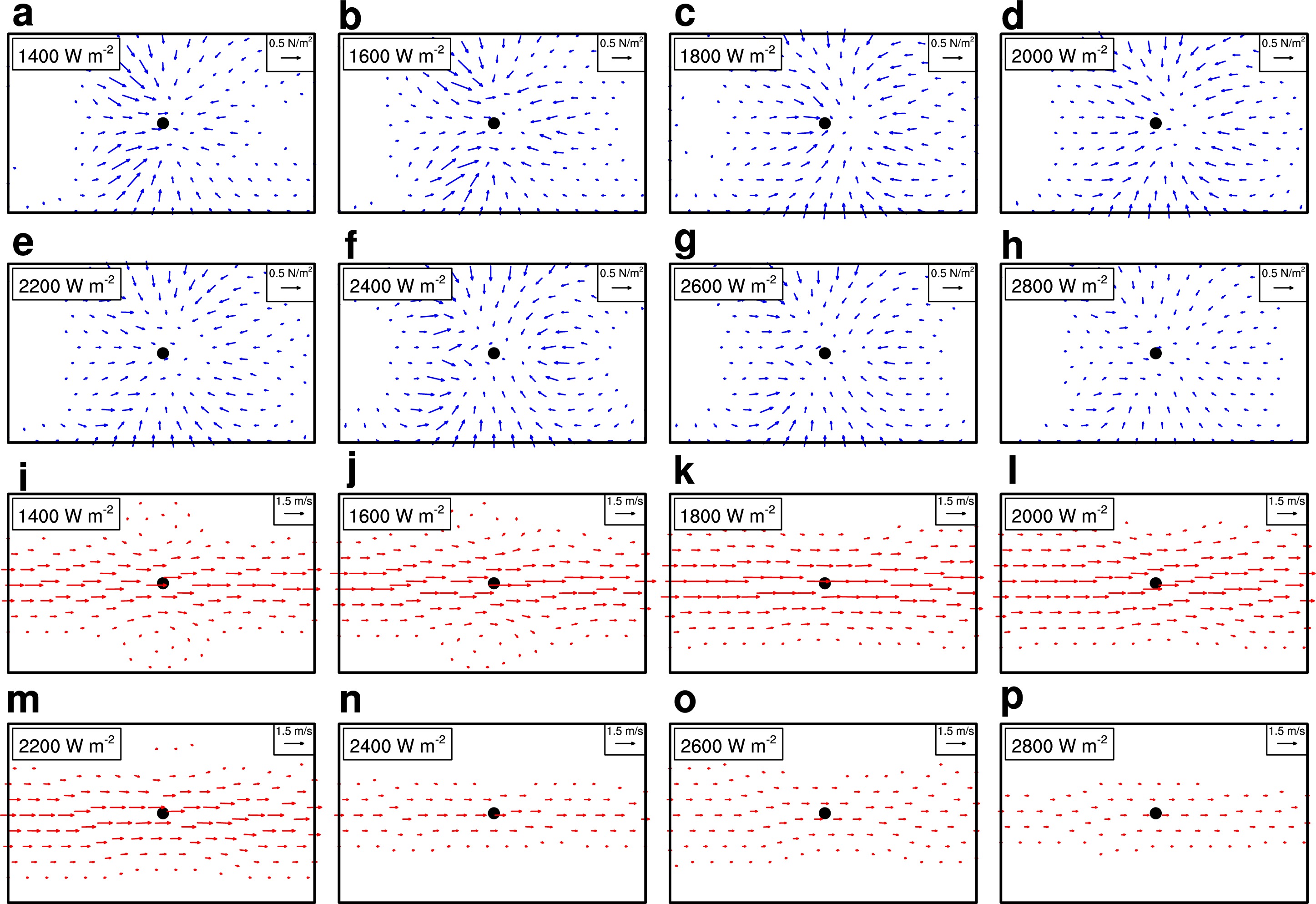
Figure 5: The 1^st reason for the weakening trend of ocean heat transport with increasing stellar flux: wind stresses weaken. Surface wind stresses on the ocean (a-f) and vertically averaged ocean currents (g-l) on tidally locked aqua-planets, as simulated by CCSM3. The stellar fluxes are 1,400, 1,600, 1,800, 2,000, 2,200, 2,400, 2,600, and 2,800 W m^-2. The horizontal axis is longitude from 0^∘ to 360^∘, and the vertical axis is latitude from 85^∘S to 85^∘N. The black dot is the substellar point. The reference vector for stresses is 0.5 N m^-2, and values less than 0.05 N m^-2 are not plotted. The reference vector for ocean velocity is 1.5 m s^-1, and values less than 0.15 m s^-1 are not plotted.

As the stellar flux is increased, both shortwave absorption by water vapor (Fig. 6(a)) and shortwave reflection by clouds increase (Fig. 4(i)). The increase in shortwave absorption by water vapor is primarily due to the increase in saturation vapor pressure with temperature following the Clausius-Clapeyron relation (Fig. 6(b)). The increase of shortwave reflection by clouds is due to the effect of a stabilizing cloud feedback: Greater stellar flux produces stronger substellar convection, more optically thick clouds, and a higher planetary albedo (Yang et al., 2013). This phenomenon was first found in atmosphere-only general circulation models and briefly tested in CCSM3; here we confirm that this feedback exists in a broader range of coupled ocean-atmosphere simulations. Both the increased water vapor absorption and enhanced cloud reflection lead to the surprising result that the stellar energy reaching the sea surface actually decreases as the stellar flux at the top of the atmosphere is increased (Fig. 6(c)).

For long-time mean climatology, the surface energy balance of an ice-free region can be written as: OHT $=$ R_s $-$ R_l $-$ SH $-$ LH, where R_s is net shortwave radiation flux into the surface, R_l is net longwave radiation flux from the surface to the atmosphere, SH is sensible heat flux from the surface to the atmosphere, and LH is latent heat flux from the surface to the atmosphere. All of these variables are positive as long as there is no temperature inversion (under an inversion, SH and R_l will be negative). This equation implies that OHT $<$ R_s, i.e., the maximum allowed OHT is constrained by the absorbed shortwave radiation at the sea surface, as shown in Fig. 6(d). The value of R_s decreases with increasing stellar flux (Fig. 6(c)), so that OHT should have the same trend.

Note that although the value of R_s decreases with stellar flux, the surface temperatures generally keep increasing (Fig. 4(d–e)); this is mainly due to the increasing of atmospheric greenhouse effect. The physical process can be briefly summarized follows: when the stellar flux is increased, more shortwave radiation is absorbed by water vapor (Fig. 6(a)), which acts to increase the air temperature and thereby the atmosphere is able to hold more water vapor based on the Clausius-Clapeyron relation. The increased water vapor concentration raises the greenhouse effect of the atmosphere (Fig. 7(d)) and emits more longwave radiation to the surface (Fig. 7(a)) such that the net longwave radiation at the surface decreases with stellar flux (Fig. 7(c)), warming the surface. Moreover, as the stellar flux is increased, the surface sensible heat flux generally decreases (Fig. 7(f)), which has a secondary warming effect on the surface.

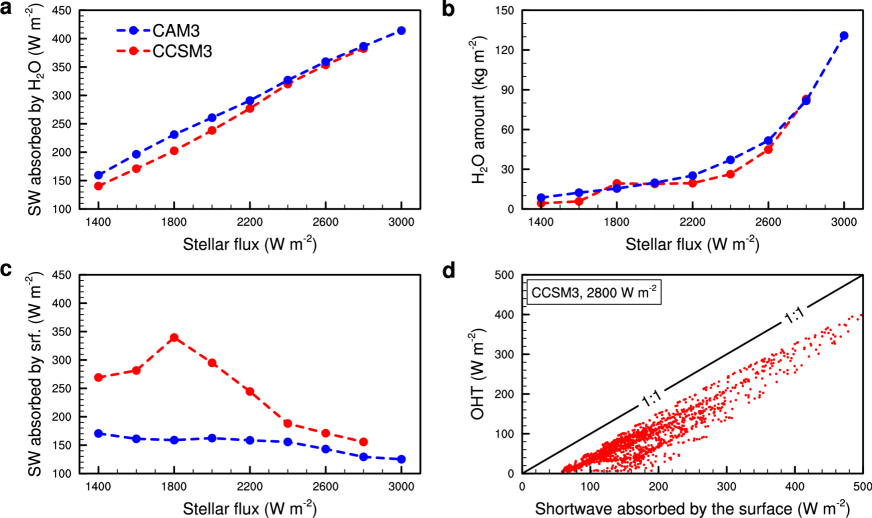
Figure 6: The 2^nd reason for the weakening trend of ocean heat transport with increasing stellar flux: surface stellar radiation decreases. Blue dot: CAM3; red dot: CCSM3. (a), shortwave (SW) radiation absorbed by water vapor on the day side; (b), vertically integrated water vapor amount on the day side; and (c), shortwave radiation absorbed by the surface (srf.) on the day side. (d), OHT vs shortwave absorbed by the surface at each grid cell of the model in CCSM3 with a stellar flux of 2,800 W m^-2; only data points that have positive values of OHT are shown. Note that OHT is smaller than the shortwave radiation absorbed by the surface for all data points; the cases of other stellar fluxes have the same relationship (figure not shown).

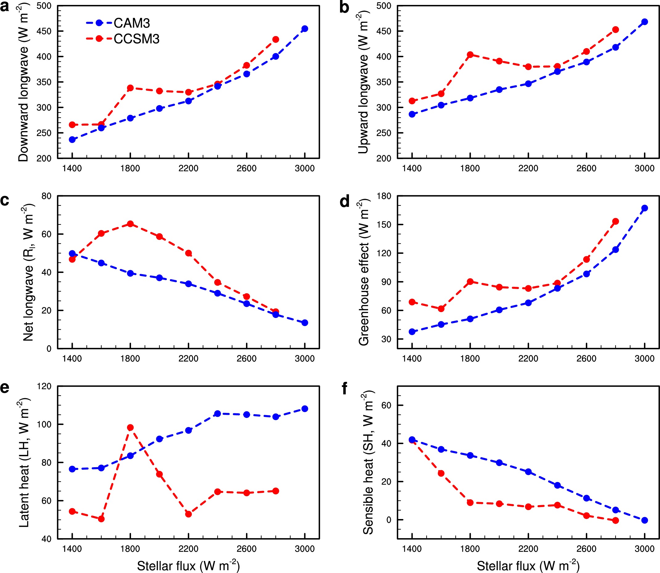
Figure 7: Surface energy flux and greenhouse effect as a function of stellar flux. (a) downward longwave radiation flux at the surface, (b) upward longwave radiation flux at the surface, (c) net longwave radiation flux (upward minus downward), (d) clear-sky greenhouse effect, defined as $\sigma T_{s}^{4}-OLR_{clear}$ where $T_{s}$ is the surface temperature, OLR_clear is the clear-sky outgoing longwave radiation at the top of the model, and $\sigma$ is the Stefan-Boltzmann constant (ref. Pierrehumbert (2005)), (e) latent heat flux at the surface, and (f) sensible heat flux at the surface. All of these variables are area averages on the day side only.

The day-to-night OHT decreases with increasing stellar flux because of the above two mechanisms, weaker surface wind stresses and less stellar energy deposited at the surface. In the 1,400 W m^-2 simulation, the OHT is 124 W m^-2, which contributes to 63 % of the total heat transport, whereas in the 2,800 W m^-2 simulation, it decreases to 70 W m^-2 and the percentage reduces to 23 % (Fig. 4(c)). These results indicate that at the inner edge of the habitable zone, the OHT would be even smaller, although the total (atmosphere plus ocean) heat transport would still be very robust.

The decreasing trend of OHT with increasing stellar flux suggests that ocean dynamics may be not important for very hot climates. Indeed, we find that the location of the inner edge of the habitable zone does not depend on ocean dynamics (Fig. 8). For a stellar temperature of 4,500 K, the climate system enters a moist greenhouse state at a stellar flux of $\simeq$ 2,600–2,800 W m^-2 for both CCSM3 and CAM3 (Fig. 8(a)). At this level of stellar flux, the stratospheric water vapor concentration, $\geq$ $3,000$ ppmv, is high enough that H₂O photo-dissociation and subsequent H escape to space becomes significant, which is known as the moist greenhouse state (Kasting, 1988; Kasting et al., 1993). It should be mentioned that at a stellar flux of 2,600 W m^-2, the day-to-night OHT is still about 25 % of the total heat transport and the difference in global-mean surface temperature between CCSM3 and CAM3 is still up to 25 K. However, the key variable for the onset of the moist greenhouse state is the stratospheric water vapor concentration rather than the global-mean surface temperature or other variable(s).

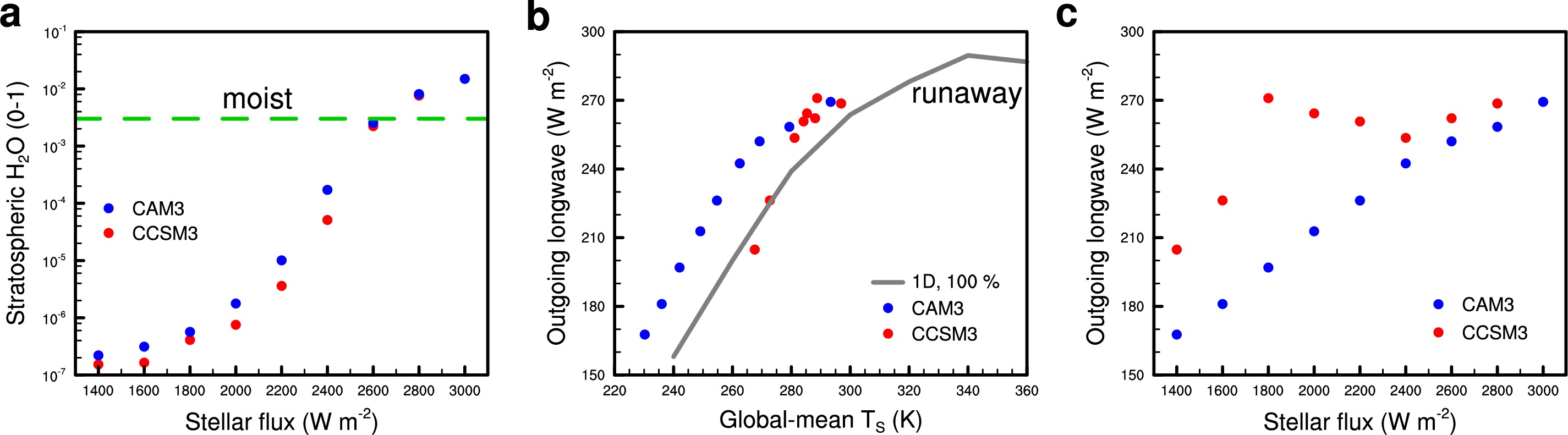
Figure 8: The effect of ocean dynamics on the inner edge of the habitable zone for a tidally locked aqua-planet around a low-mass star. Red dots: CCSM3, and blue dots: CAM3. (a), global-mean stratospheric water vapor mixing ratio at 50 hPa, as a function of stellar flux (horizontal green line: the moist greenhouse limit of 3,000 ppmv). (b), global-mean outgoing longwave radiation (OLR) as a function of surface temperature. The gray line in (b) is the OLR from a 1D cloud-free radiative transfer model assuming 100 % relative humidity, as calculated by Leconte et al. (2013a). (c) OLR as a function of stellar flux.

For lower stellar fluxes, stratospheric water vapor in CCSM3 is slightly lower than in CAM3 (Fig. 8(a)), due to relatively weaker vertical velocities in the stratosphere over the substellar region in CCSM3 than those in CAM3 (figure not shown). At higher stellar flux, however, the day-to-night OHT become weaker and the two models have the same concentration of stratospheric water vapor. On tidally locked planets, the stratospheric water vapor abundance is primarily determined by the temperature of the tropopause and the strength of the stratospheric vertical velocity above the substellar region. The vertical velocity is mainly driven by near-infrared radiative heating associated with shortwave absorption by stratospheric water vapor and cloud particles (Fujii et al., 2017).

Finally, our results suggest that the ocean-atmosphere and atmosphere-only models would enter into a runaway greenhouse state, in which absorbed shortwave exceeds maximum allowed outgoing longwave ($OLR_{max}$), at a similar stellar flux. The stellar flux limit (S_limit) for triggering the runaway greenhouse only depends on $OLR_{max}$ and the planetary albedo near the inner edge ($\alpha_{p}$), i.e., S_limit = $4\times OLR_{max}/(1-\alpha_{p})$, where the factor 4 is the ratio of a sphere’s surface area to its cross-sectional area. Figure 8(b) shows that the two models likely have the same $OLR_{max}$. Meanwhile, they exhibit nearly the same $\alpha_{p}$ as the stellar flux is increased to 2,800 W m^-2 (Fig. 4(i)), although the global-mean surface temperature still has a difference of 20 K and the day-to-night OHT is still 23 % of the total heat transport. In the models we used, the stellar flux limit is about 3,300 W m^-2 both with and without ocean dynamics. This limit is about two times that for rapidly rotating planets around G stars (such as Earth, Leconte et al. (2013a)), primarily due to the stabilizing cloud feedback (Yang et al., 2013). In summary, ocean dynamics do not influence the stellar flux limit for the onset of the runaway greenhouse state in our experiments using a 60-day tidally locked orbit.

As shown in Fig. 8(b), for lower stellar fluxes and under the same global-mean surface temperature, outgoing longwave radiation at the top of the model in CAM3 is higher than in CCSM3. This is due to the absence of a nightside temperature inversion (Fig. 2(f)) and the stronger longwave cloud radiative effect in CCSM3 (Fig. 3), both of which reduce the outgoing longwave radiation in the coupled atmosphere-ocean model. When the stellar flux is $\geq$ 3,000 W m^-2, the temperature inversion in CAM3 disappears and the longwave cloud radiative effect becomes close to that of CCSM3 (Fig. 3(b)), so that the outgoing longwave radiation fluxes of the two models coverge to each other (Fig. 8(b)). Note that due to numerical instability, CCSM3 blew up for stellar fluxes higher than 2,800 W m^-2, so that the maximum allowed outgoing longwave radiation can not be read from Fig. 8(b), however, our present experiments show no evidence that ocean dynamics affects the maximum allowed outgoing longwave radiation and the planetary albedo at the inner edge of the habitable zone.

Another way to understand the differences and similarities between CAM3 and CCSM3 is plotting the global-mean outgoing longwave radiation as a function of the stellar radiation downward at the top of the atmosphere, as shown in Fig. 8(c). At equilibrium, outgoing longwave radiation is equal to absorbed stellar radiation. At lower stellar fluxes, the outgoing longwave radiation is higher in CCSM3 than in CAM3 because CCSM3 has a lower planetary albedo (see Fig. 4(i)) and therefore absorbs more stellar radiation. For a high stellar flux, $\geq$2,400 W m^-2, the difference in the outgoing longwave radiation between CAM3 and CCSM3 becomes small; this again suggests that ocean dynamics likely have no significant effect on the inner edge of the habitable zone.

3.3 Observational Thermal Phase Curves

We further find that ocean dynamics have a very small effect on the observational thermal phase curve of tidally locked planets near the inner edge of the habitable zone. Figure 9 shows the spatial pattern of thermal emission at the top of the atmosphere and thermal phase curves. The phase curves are disk-integrated thermal radiation measured by an observer as a function of the planet’s position in its orbit (e.g., Cowan & Agol, 2008; Koll & Abbot, 2015). The curves are determined by the combined effect of surface temperature, water vapor, clouds, and atmospheric and oceanic heat transports; therefore, they can be used to probe the atmosphere and/or surface characteristics of exoplanets.

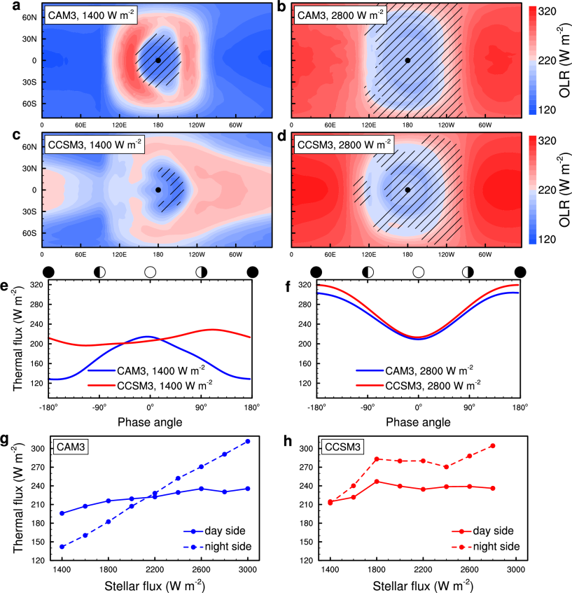
Figure 9: Effects of ocean dynamics on thermal phase curves of planets in the middle range (left columns) and near the inner edge (right columns) of the habitable zone. (a-d), outgoing longwave radiation (OLR, color shading) and vertically integrated cloud water content higher than 400 g m^-2 (masked by oblique lines). (a), CAM3’s simulation with a stellar flux of 1,400 W m^-2; (b), CAM3 and 2,800 W m^-2; (c), CCSM3 and 1,400 W m^-2; and (d), CCSM3 and 2,800 W m^-2. (e), thermal phase curves of CAM3 (blue line) and CCSM3 (red line) with a stellar flux of 1,400 W m^-2. (f), same as (e) but for 2,800 W m^-2. The observer views the day side of the planet at a phase angle of 0^∘ and sees the night side at phase angles of $\pm$180^∘. (g), time-mean thermal flux on the day side (solid line) and the night side (dashed line) in CAM3. (h), same as (g) but for CCSM3. Note in (a-d), due to the effect of clouds and water vapor, there is a decrease in OLR over the substellar point in all experiments.

For planets near the inner edge of the habitable zone, the day-to-night OHT is not strong, so that the phase curves of CAM3 and CCSM3 are similar (Fig. 9(f)). Importantly, the thermal emission on the night side is much higher than that on the day side, reversing the day-night thermal contrast (Fig. 9(b,d)). This reversal is due to the high concentration of water vapor and clouds above the substellar region, which absorb the thermal radiation from the surface but re-emit to space at much lower temperatures (Yang et al., 2013; Haqq-Misra et al., 2017). Meanwhile, the night side is relatively dryer and therefore infrared radiation from near the surface can be lost to space easily (Yang & Abbot, 2014b; Pierrehumbert, 1995). In CAM3, the phase curve reversal occurs when the stellar flux is equal to or higher than 2,200 W m^-2 whereas in CCSM3 it occurs at a much lower stellar flux, 1,600 W m^-2 (Fig. 9(g,h)). This suggests that planets with deep oceans in the middle range of the habitable zone could also have higher thermal emission on the night side than on the day side.

For a stellar flux of 1,400 W m^-2 in CAM3, the phase curve has a maximum when the observer sees the day side and a minimum when the observer views the night side (Fig. 9(e)). When ocean dynamics are included, more heat is transported to the night side, so that the day-night thermal contrast in CCSM3 is much smaller than that in CAM3 and therefore the amplitude of the phase curve is much smaller. Furthermore, because most of the heat is transported to the east side (rather than the west side) of the substellar point (Fig. 9(c)), the ridge of the phase curve exhibits a positive phase angle displacement of $\simeq$ 120^∘ (Fig. 9(e)). In contrast, when ocean dynamics are not considered, the thermal emission on the west side of the substellar point is relatively higher than that on the east side (Fig. 9(a)), because water vapor is transported eastward, where it absorbs thermal emission from the surface, and therefore the thermal phase curve exhibits a small negative phase angle displacement (Fig. 9(e), see also Fig. 3(b) in Yang et al. (2013)).

Could the oceanic effect on the thermal phase curve be observed by the James Webb Space Telescope (JWST)? To estimate JWST’s precision, we assume that observations are only limited by photon noise and by the telescope’s detector efficiency (see Koll & Abbot (2015)). For the target we assume the LHS 1140 system (Dittmann et al., 2017); closer or brighter host stars would be easier to measure. For the instrument we assume MIRI-F1800W (16.5-19.5 micron) photometry and a photon efficiency of $1/3$. Because habitable zone planets are cool, it is necessary to observe at long wavelengths to obtain favorable planet-star thermal contrasts. We note that at such long wavelengths additional sources of error could become significant, e.g., dust or thermal background, so our estimate is optimistic. For a 2-hour integration the 1 sigma error bar for the flux will be 144 W m^-2. For a 24-hour integration, the error goes down by $1/\sqrt{12}$, so a 1 sigma error would be $\simeq$42 W m^-2, larger than the amplitude of the thermal phase curve shift under ocean dynamics in the middle of the habitable zone (see red line in Fig. 9(e)) but smaller than the amplitude of the day-night phase curve reversal near the inner edge of the habitable zone (Fig. 9(f)). Therefore, JWST observations with long staring exposures would be able to detect the thermal phase curve reversal near the inner edge of the habitable zone. However, unless future discoveries detect a target more favorable than LHS 1140b, the ocean-induced thermal phase shift would likely not detectable with JWST.

3.4 Non-monotonic Behavior of the Coupled Atmosphere–Ocean System

As shown in Figs. 3, 4, 6 and 7, the climate in CCSM3 is not a monotonic function of stellar flux. Variables that show the non-monotonic behavior include: (1) the day-to-night ocean heat transport (Fig. 4(a)), night-side longwave cloud radiative effect (Fig. 3(b)), day-side shortwave absorption by the sea surface (Fig. 6(c)), and surface net longwave radiation (Fig. 7(c)) increase with stellar flux between 1,400 and 1,800 W m^-2 but decrease with stellar flux when it is higher than 1,800 W m^-2; (2) the global-mean surface temperature (Fig. 4(d)), day-to-night total heat transport (Fig. 4(b)), global-mean longwave cloud radiative effect (Fig. 3(a)), and both upward and downward longwave radiation fluxes at the surface (Fig. 7(a & b)) increase between 1,400 and 1,800 W m^-2, decrease between 1,800 and 2,400 W m^-2, and increase again when the stellar flux is higher than 2,400 W m^-2; (3) the planetary albedo (Fig. 4(i)) mostly increases with stellar flux but has a minimum value when the stellar flux is 1,800 W m^-2. Sensitivity tests show that this non-monotonic behavior seems don’t depend on the initial state (Fig. 1(e-f)).

The non-monotonic behavior in CCSM3 likely results from atmosphere–ocean interactions and associated feedback processes because the climate simulated using the atmosphere-only model CAM3 is close to monotonic (see Figs. 3,  4, 6, & 7). The increase in global-mean surface temperature between 1,400 and 1,600 W m^-2 and between 2,400 and 2,800 W m^-2 in CCSM3 is relatively easier to understand, whereas the slight decrease in global-mean surface temperature between 1,800 and 2,200 W m^-2 and the minimum in planetary albedo at 1,800 W m^-2 are due to the complex interactions between the ocean, atmosphere and clouds. Comparing the 1,400 and 1,600 W m^-2 cases, the night side is covered by sea ice in both experiments (Fig. 10(b)) and the surface temperature gradients decrease but not very significantly (Figs. 10(a) & 4(f-g)), so that the OHT increases with increasing stellar flux. This implies that in these two experiments of relatively lower stellar flux the two mechanisms—the surface temperature gradient decreasing and the surface wind stress weakening addressed in the section 3.2 are not active enough to counteract the effect of increasing stellar flux. In the 2,400, 2,600 and 2,800 W m^-2 experiments, the two mechanisms are very effective in reducing the day-to-night OHT although the stellar flux is increased and the atmospheric heat transport increases with stellar flux; as shown in Fig. 5, the ocean currents in these three cases are much weaker than those in all other experiments. For the cases between 1,800 and 2,200 W m^-2, the situation is more complex and the key may be associated with the effect of ocean dynamics on the spatial pattern of sea surface temperature and consequently on the atmospheric heating rate, the strength of atmospheric superrotation (winds blowing from west to east over the deep-tropical region) and the spatial pattern of clouds (Fig. 10). In the 1,800 W m^-2 case of CCSM3, strong ocean currents transport relatively cold seawater from the night side to the west side of the substellar point and also transport relatively warm seawater from the substellar point to its east side (similar behavior also occurs at 2,000 and 2,200 W m^-2, but the 1,800 W m^-2 case is the most significant). As a result, the sea surface temperature exhibits a strong, zonally asymmetric pattern with the east side of the substellar point much warmer than the west side (Fig. 10(a)). This asymmetric pattern causes the water vapor concentration and atmospheric heating rate to show a similar zonally asymmetric pattern (Fig. 10(c-d)). The asymmetric heating pattern is likely more effective at generating Rossby waves and Kelvin waves in the atmosphere; the waves pump eastward momentum from higher latitudes to the equator (Showman & Polvani, 2011), inducing very strong super-rotating winds over the substellar region (Fig. 10(e & j)); these winds advect clouds eastward away from the substellar region where the stellar flux peaks, and the west side of the substellar point becomes nearly cloud-free (Fig. 10(f)); as a result, the planetary albedo becomes smaller (0.39 in the case of 1,800 W m^-2 versus 0.44 in the case of 1,600 W m^-2, suggesting that the stabilizing cloud feedback is less active for this case); therefore, more stellar radiation reaches the surface, warming the sea surface. In CAM3, this phenomenon does not occur because the day-side sea surface temperature is nearly symmetric around the substellar point and the atmospheric zonal winds are weak in all of the experiments (Fig. 11).

Moreover, in CCSM3 the strength of the atmospheric super-rotation decreases with stellar flux between 1,800 and 2,200 W m^-2 (Fig. 10(j)), so that the planetary albedo increases with stellar flux, which enhances the primary effect of the stabilizing cloud feedback with increasing stellar flux (Yang et al., 2013). The planetary albedo increases with stellar flux fastest in these three experiments (Fig. 4(i)) and as a result the global-mean surface temperature decreases sightly (rather than increases) with stellar flux (Fig. 4(d)). The decrease in OHT of these three experiments is due to the combined effect of the planetary albedo increasing (so less surface shortwave radiation is deposited) and surface wind stress weakening (Figs. 4(h) & 5). Further work is required to clearly understand the onset condition for strong atmospheric super-rotation in the coupled model, especially as relates to the role of the spatial pattern of surface temperature or atmospheric heating.

Overall, the non-monotonicity of CCSM3 is likely due to complex interactions among the sea surface, atmospheric circulation, water vapor and clouds. This further demonstrates that why fully coupled atmosphere-ocean modeling is required to simulate the details of the climate of planets in the middle of the habitable zone.

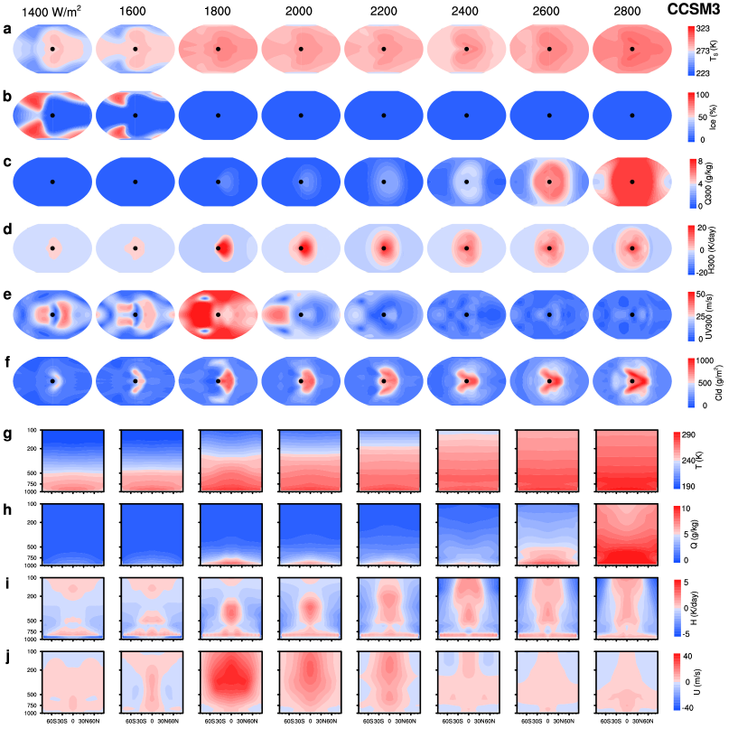
Figure 10: Atmospheric characteristics simulated by CCSM3 at stellar fluxes from 1,400 to 2,800 W m^-2 with an interval of 200 W m^-2. (a) Surface air temperature, (b) sea ice coverage, (c) water vapor specific humidity at 300 hPa, (d) heating rate at 300 hPa due to the combined effect of shortwave heating, longwave cooling, and moist processes (such as latent heat release during condensation), (e) horizontal wind strength ($\sqrt{u^{2}+v^{2}}$) at 300 hPa, (f) vertically integrated cloud water amount, (g) zonal-mean air temperature, (h) zonal-mean water vapor specific humidity, (i) zonal-mean heating rate, and (j) zonal-mean zonal winds. Note that the troposphere and water vapor profiles extend to higher altitudes in a warmer climate, so that more stellar radiation is absorbed by water vapor at high altitudes. The black dot in (a–f) denotes the substellar point.

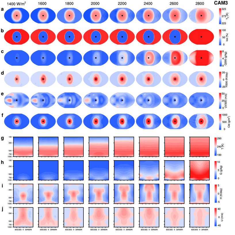
Figure 11: Same as Fig. 10 but CAM3 simulations.

4 Discussion

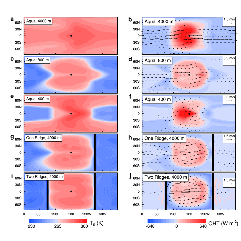
Figure 12: Effects of ocean depth and continental barriers on the long-time mean surface temperature (left panels) and ocean heat transport (OHT, right panels, negative: heat from ocean to atmosphere, positive: heat from atmosphere to ocean). (a & b), an aqua-planet with an uniform ocean depth of 4,000 m; (c & d), an ocean depth of 800 m; (e & f), an ocean depth of 400 m; (g & h), one-ridge world with an ocean depth of 4,000 m; and (i & j), two-ridges world with an ocean depth of 4,000 m. In the right panels, the vectors denote vertically averaged ocean currents with reference vectors of 1.5, 0.3, 0.3, 1.5, and 1.5 m s^-1, respectively. The thick black lines in (g-j) denote the continental barriers, which extend from the ocean bottom to the sea surface. The black dot denotes the substellar point. In these simulations, the stellar temperature is 3,400 K, the stellar flux is 1,400 W m^-2, and the planetary rotation period is 37 Earth days (see Table 1).

An important result of this study is that the location of the habitable zone’s inner edge should not depend significantly on ocean dynamics. This is consistent with Way et al. (2018), who found that the effect of ocean dynamics on the climate decreases rapidly with stellar flux for a variety of rotation rates in the ROCKE3D GCM (their Fig. 2). We should note, however, our experiments cover a limited range of planetary parameters. We have examined the dynamics of an aqua-planet ocean having a depth of $\simeq$ 4,000 m. Sensitivity tests show that at a stellar flux of 1,400 W m^-2 for shallower oceans or for oceans surrounded by continents, the day-to-night OHT would become smaller and its climatic effect would be weaker (Fig. 12). For a shallower ocean, friction at the ocean bottom is more effective at decelerating ocean currents, so that less warm substellar seawater can be transported to the cold night side. In the case of an 800-m deep ocean, the night side is much cooler than that in the 4,000-m case as a result of less ocean heat input from the day side. The dayside surface, however, also becomes cooler even though less energy is transported away from the substellar region. This is due to a cloud feedback. Due to the reduced OHT (Fig. 12(d)), the surface temperature contrast between the day side and the night side increases (Fig. 12(c)). The larger surface temperature contrast promotes stronger water vapor convergence above the substellar region, and therefore more clouds form there. These clouds have a strong cooling effect on the sea surface through increasing planetary albedo. The planetary albedos are 0.29 and 0.45 in the cases of 4,000 and 800 m, respectively. When the ocean depth is 400 m, the zonal (West-East) ocean currents become weaker (compared to the 800 m case), so that less energy is transported to the night side through ocean dynamics (Fig. 12(f)); however, the meridional (North-South) oceanic heat transport increases, so that the high latitudes become warmer (Fig. 12(e)), similar to the results of Del Genio et al. (2019). Compared the 4,000-m aqua-planet, the trends in the one barrier case and the two barriers case are similar to the 800-m aqua-planet case: The day-to-night ocean heat transport reduces and both dayside and nightside surfaces become cooler (Fig. 12(g-h)). In the two barriers case, the day-to-night OHT is completely blocked by the continents and the ocean currents can transport the substellar heat only to the terminators and to the day-side polar regions, where the surface becomes warmer than in the one barrier case (Fig. 12(i-j)). Future work is required to further investigate the ocean barrier cases, as well as more ocean depth cases, under higher stellar fluxes.

Future work is also required to investigate the effects of ocean dynamics on planets in different spin-orbit resonance states (such as 3:2 for Mercury), on rapidly rotating planets around G stars (such as Earth) and on planets near the outer edge of the habitable zone, as well as the effects of different atmospheric masses, atmospheric compositions and of deeper oceans (such as ocean worlds, Leger et al., 2003). A higher background atmospheric pressure than the one bar used in this study may further lessen the surface shortwave energy deposition through increasing atmospheric scattering, which may further weaken the effect of ocean dynamics on the inner edge of the habitable zone. A lower background atmospheric pressure should have a small effect on the results shown here because water vapor should dominate atmospheric composition at the inner edge of the habitable zone, especially for the runaway greenhouse state.

In our experiments, the salinity of sea ice is set to 4 g kg^-1 while the seawater salinity is about 35 g kg^-1, so that sea ice melting and freezing is able to influence the ocean salinity and thereby oceanic thermohaline circulation. The thermohaline circulation has not been shown in this manuscript because the day-to-night OHT is dominated by wind-driven ocean circulations in our experiments. Our model blew up when the stellar flux was higher than 2,800 W m^-2. Future experiments are required for higher stellar fluxes, under which wind-driven ocean circulation would become even weaker and thermohaline circulation might become important. Our preliminary thinking is that for planets near the inner edge of the habitable zone, the thermohaline circulation should be mainly driven by the salinity gradient because the surface temperature gradient is very small. The salinity gradient is mainly determined by the spatial pattern of precipitation and evaporation that are driven by large-scale atmospheric circulation. For planets at the outer edge of the habitable zone, the thermohaline circulation may be larger than that at the inner edge. This is because both temperature and salinity gradients on planets at the outer edge may be strong enough to drive a robust thermohaline circulation. Cullum et al. (2014, 2016) examined the effects of planetary rotation and average ocean salinity on the thermohaline circulation using an ocean-only model. Wind-driven ocean circulation and the interactions between ocean, atmosphere and surface climate, however, were not considered in their studies. Future work is required to examine the effect of average ocean salinity on the ocean circulation (as was briefly tested in Del Genio et al. (2019) for Proxima b) and the effect of thermal-driven ocean circulation on the inner and outer edges of the habitable zone.

5 Summary

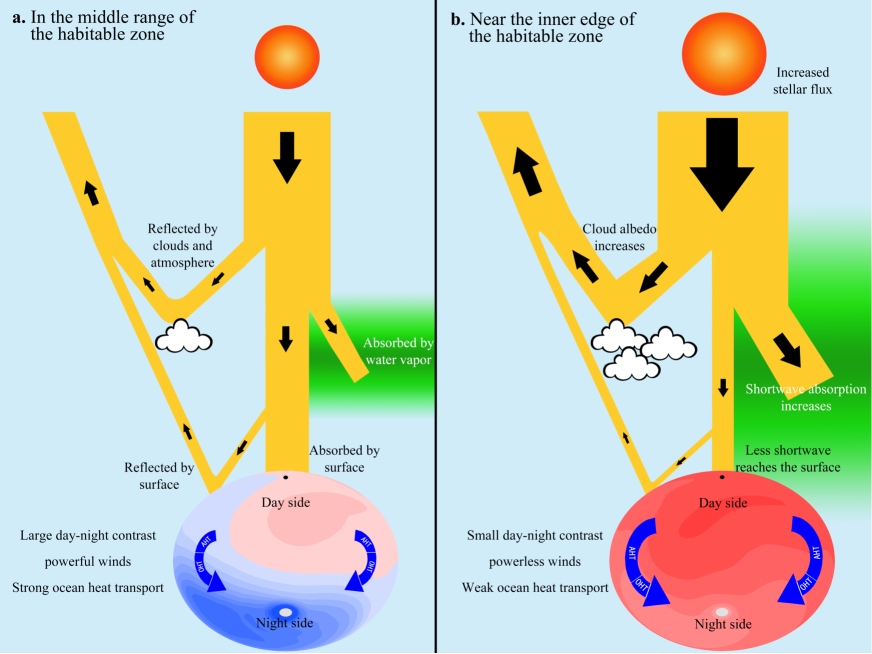
Figure 13: Schematic illustration of the decrease in day-to-night ocean heat transport (OHT) as the stellar flux increases and the underlying mechanisms. The decreasing trend of OHT results from weaker wind stress combined with less stellar radiation depositing energy at the dayside surface. (a): In the middle range of the habitable zone, the day-night surface temperature contrast is strong, the surface wind stresses are robust, stellar radiation absorbed by water vapor or reflected by clouds is relatively small, a large part of the stellar energy reaches the surface, and the ocean dominates the day-to-night heat transport. (b): Near the inner edge of the habitable zone, the surface is hot, the day-night surface temperature contrast is small, the surface wind stresses are weak, stellar radiation absorbed by water vapor or reflected by clouds is relatively large, a small part of the stellar energy reaches the surface, and the atmosphere dominates the day-to-night heat transport.

In the middle range of the habitable zone, ocean dynamics significantly warm the night side and the dayside high latitudes of 1:1 tidally locked aqua-planets and produce an eastward shift of the hottest point at the surface. For planets near the inner edge of the habitable zone, however, oceanic heat transport is weak and has nearly no effect on the location of the inner edge or on the thermal phase curves of planets near the inner edge (summarized in Fig. 13). The weakening of oceanic heat transport with increasing stellar flux is due to the combined effect of weakened surface wind stress and decreased surface stellar energy deposition at the sea surface. Atmospheric heat transport increases with stellar flux and dominates on planets near the inner edge of the habitable zone. Finally, we note that the detection of oceans, continents and atmospheres on distant terrestrial exoplanets is still a big challenge (e.g., Cowan et al., 2009, 2012a, 2012b). Future observations using high temporal frequency specular reflections as well as emission and transmission spectra may be able to infer the surface as well as atmospheric characteristics of nearby transiting planets (Cowan et al., 2015; Greene et al., 2016; Stevenson et al., 2016; Bean et al., 2018).

References

- Bean et al. (2018) Bean, J. L., Stevenson, K. B., Batalha, N. M., Berta-Thompson, Z., Kreidberg, L., et al. 2018, Publications of the Astronomical Society of the Pacific, 130, 11402
- Bin et al. (2018) Bin, J., Tian, F., & Liu, L. 2018, Earth Planet. Sci. Lett., 492, 121
- Boutle et al. (2017) Boutle, I. A., Mayne, N. J., Drummond, B., Manners, J., Goyal, J., Lambert, F. H., Acreman, D. M., & Earnshaw, P. D. 2017, Astronomy & Astrophysics, 601, A120
- Briegleb et al. (2002) Briegleb, B., Bitz, C. M., Hunke, E. C., Lipscomb, W. H., & Schramm, J. L. 2002, Description of the community climate system model version 2 sea ice model, http://www.ccsm.ucar.edu/models/ice-csim4
- Collins et al. (2006) Collins, W. D., Bitz, C. M., Blackmon, M. L., Bonan, G. B., et al. 2006, The Community Climate System Model version 3 (CCSM3)
- Collins et al. (2004) Collins, W. D., et al. 2004, Description of the NCAR community atmosphere model (CAM 3.0), http://www.cesm.ucar.edu/models/atm-cam/docs/description/description.pdf
- Cowan et al. (2012a) Cowan, N. B., Abbot, D. S., & Voigt, A. 2012a, Astrophysical Journal Letters, 752, L3, doi:10.1088/2041-8205/752/1/L3
- Cowan et al. (2012b) —. 2012b, Astrophysical Journal, 757, 80, doi:10.1088/0004-637X/757/1/80
- Cowan & Agol (2008) Cowan, N. B., & Agol, E. 2008, Astrophys J, 678, 129
- Cowan et al. (2015) Cowan, N. B., Greene, T., Angerhausen, D., Batalha, N. E., Clampin, M., Colon, K., et al. 2015, Publications of the Astronomical Society of the Pacific, 127, 311
- Cowan et al. (2009) Cowan, N. B., et al. 2009, Astrophys J, 700, 915, doi:10.1088/0004-637X/700/2/915
- Cullum et al. (2014) Cullum, J., Stevens, D. P., & Joshi, M. 2014, Astrobiology, 14, 645
- Cullum et al. (2016) —. 2016, Proc. Natl. Acad. Sci., 113, 4278
- Del Genio et al. (2019) Del Genio, A. D., Way, M. J., Amundsen, D. S., Aleinov, I., Kelley, M., Kiang, N. Y., & Clune, T. L. 2019, Astrobiology, 1, doi:10.1089/ast.2017.1760
- Dittmann et al. (2017) Dittmann, J. A., Irwin, J. M., Charbonneau, D., Bonfils, X., Astudillo-Defru, N., Haywood, R. D., et al. 2017, Nature, 544, 333
- Edson et al. (2011) Edson, A., Lee, S., Bannon, P., Kasting, J. F., & Pollard, D. 2011, Icarus, 212, 1, DOI:10.1016/j.icarus.2010.11.023
- Enderton & Vallis (2009) Enderton, R., & Vallis, G. K. 2009, J. Atmos. Sci., 66, 1593
- Farneti & Vallis (2013) Farneti, R., & Vallis, G. K. 2013, J. Climate, 26, 7151
- Fujii et al. (2017) Fujii, Y., Genio, D. A. D., & Amundsen, D. S. 2017, Astrophysical Journal, 848, 100
- Gent & McWilliams (1990) Gent, P. R., & McWilliams, J. C. 1990, J. Phys. Oceanogr., 20, 150
- Greene et al. (2016) Greene, T. P., Line, M. R., Montero, C., Fortney, J. J., Lustig-Yaeger, J., & Luther, K. 2016, The Astrophysical Journal, 817, 1
- Haqq-Misra et al. (2017) Haqq-Misra, J., Wolf, E. T., Joshi, M., Zhang, X., Kopparapu, R. K., et al. 2017, The Astrophysical Journal, 852, 1
- Hartmann (2016) Hartmann, D. 2016, Global Physical Climatology (Elsevier publication, San Diego), 409
- Herweijer et al. (2005) Herweijer, C., Seager, R., Winton, M., & Clement, A. 2005, Tellus, 57, 662
- Hu & Yang (2014) Hu, Y., & Yang, J. 2014, Proceedings of the National Academy of Sciences, 111, 629
- Joshi et al. (1997) Joshi, M., Haberle, R., & Reynolds, R. 1997, Icarus, 129, 450
- Joshi & Haberle (2012) Joshi, M. M., & Haberle, R. M. 2012, Astrobiology, 12, 3
- Kasting (1988) Kasting, J. F. 1988, Icarus, 74, 472
- Kasting et al. (1993) Kasting, J. F., Whitmire, D. P., & Reynolds, R. T. 1993, Icarus, 101, 108
- Koll & Abbot (2013) Koll, D. D., & Abbot, D. S. 2013, Journal of Climate, 26, 6742
- Koll & Abbot (2015) Koll, D. D. B., & Abbot, D. S. 2015, The Astrophysical Journal, 802, 21, doi:10.1088/0004-637X/802/1/21
- Kopparapu et al. (2017) Kopparapu, R. K., Wolf, E. T., Arney, G., Batalha, N. E., Haqq-Misra, J., Grimm, S. L., & Heng, K. 2017, The Astrophysical Journal, 845, 5
- Kopparapu et al. (2016) Kopparapu, R. K., Wolf, E. T., Haqq-Misra, J., Yang, J., Kasting, J. F., Meadows, V., Terrien, R., & Mahadevan, S. 2016, The Astrophysical Journal, 819, 84
- Large et al. (1990) Large, W. G., McWilliams, J. C., & Doney, S. C. 1990, J. Phys. Oceanogr., 27, 2418
- Leconte et al. (2013a) Leconte, J., Forget, F., Charnay, B., Wordsworth, R., & Pottier, A. 2013a, Nature, 504, 268
- Leconte et al. (2013b) Leconte, J., Forget, F., Charnay, B., Wordsworth, R., Selsis, F., Millour, E., & Spiga, A. 2013b, Astronomy And Astrophysics, 554, A69
- Leger et al. (2003) Leger, A., et al. 2003, Icarus, 169, 499
- Liu et al. (2013) Liu, Y., Peltier, W., Yang, J., & Vettoretti, G. 2013, Climate Of The Past, 9, 2555
- Marcq et al. (2017) Marcq, E., Salvador, A., Massol, H., & Davaille, A. 2017, J. Geophys. Res. Planets, 122, 1539
- Marshall et al. (2007) Marshall, J., Ferreira, D., Campin, J. M., & Enderton, D. 2007, J. Atmos. Sci., 64, 4270
- Merlis & Schneider (2010) Merlis, T. M., & Schneider, T. 2010, Journal of Advances in Modeling Earth Systems, 2, 1
- Pierrehumbert (1995) Pierrehumbert, R. T. 1995, Journal of the Atmospheric Sciences, 52, 1784
- Pierrehumbert (2005) —. 2005, JGR-atmospheres, 110, D01111, doi:10.1029/2004JD005162
- Pierrehumbert (2011) —. 2011, Astrophys J Lett, 726, L8, doi:10.1088/2041-8205/726/1/L8
- Popp et al. (2016) Popp, M., Schmidt, H., & Marotzke, J. 2016, Nature Communications, 7, 10627
- Rosenbloom et al. (2011) Rosenbloom, N., Shields, C. A., Brady, E., Yeager, S., & Levis, S. 2011, Using CCSM3 for Paleoclimate Applications, http://opensky.ucar.edu/islandora/object/technotes%3A496/datastream/PDF/view
- Salameh et al. (2017) Salameh, J., Popp, M., & Marotzke, J. 2017, Climate Dynamics, 50, 1
- Shields et al. (2013) Shields, A. L., Meadows, V. S., Bitz, C. M., Pierrehumbert, R. T., Joshi, M. M., & Robinson, T. D. 2013, Astrobiology, 13, 715
- Showman & Polvani (2011) Showman, & Polvani, L. M. 2011, Astrophys. J., 738, 71
- Smith & Gent (2004) Smith, R., & Gent, P. 2004, Ocean component of the Community Climate System Model (CCSM2.0 and 3.0), http://www.cesm.ucar.edu/models/ccsm3.0/pop/doc/manual.pdf
- Smith & McWilliams (2003) Smith, R. D., & McWilliams, J. C. 2003, Ocean Modelling, 5, 129
- Smith et al. (2006) Smith, R. S., Dubois, C., & Marotzke, J. 2006, J. Climate, 19, 4719
- Stevenson et al. (2016) Stevenson, K. B., Lewis, N. L., Bean, J. L., Beichman, C., Fraine, J., Kilpatrick, B. M., et al. 2016, Publications of the Astronomical Society of the Pacific, 128, 094401
- Turbet et al. (2016) Turbet, M., Leconte, J., Selsis, F., Bolmont, E., Forget, F., Ribas, I., Raymond, S. N., & Anglada-Escudé, G. 2016, Astronomy & Astrophysics, 596, A112
- Turbet et al. (2018) Turbet, M., et al. 2018, Astronomy & Astrophysics, 612, 1
- Vallis (2006) Vallis, G. K. 2006, Atmospheric and Oceanic Fluid Dynamics (Cambridge, U.K.: Cambridge University Press), 745
- Vallis (2012) —. 2012, Climates and the Oceans (Princeton, U.S.A.: Princeton University Press), 245
- Vallis & Farneti (2009) Vallis, G. K., & Farneti, R. 2009, Terra Nova, 135, 1643
- Vogt et al. (2010) Vogt, S. S., Butler, R. P., Rivera, E. J., Haghighipour, N., Henry, G. W., & Williamson, M. H. 2010, Astrophys J, 723, 954, doi:10.1088/0004-637X/723/1/954
- Wang et al. (2014) Wang, Y., Feng, T., & Hu, Y. 2014, ApJ, 791, L12, doi:10.1088/2041-8205/791/1/L12
- Wang et al. (2016) Wang, Y., Liu, Y., Feng, T., Yang, J., Ding, F., Zhou, L., & Hu, Y. 2016, ApJ, 823, L20, doi:10.3847/2041-8205/823/1/L20
- Watson et al. (2015) Watson, A. J., Vallis, G. K., & Nikurashin, M. 2015, Nature Geoscience, 8, 861
- Way et al. (2018) Way, M. J., Del Genio, A., Aleinov, I., Clune, T., Kelley, M., & Kiang, N. Y. 2018, arXiv:1808.06480
- Way et al. (2015) Way, M. J., Del Genio, A., Kelley, M., Aleinov, I., & Clune, T. 2015, arXiv preprint arXiv:1511.07283
- Way et al. (2016) Way, M. J., Del Genio, A. D., Kiang, N. Y., Sohl, L. E., Grinspoon, D. H., Aleinov, I., Kelley, M., & Clune, T. 2016, Geophysical Research Letters, 43, 8376
- Winton (2003) Winton, M. 2003, Journal of Climate, 16, 2875
- Wolf & Toon (2015) Wolf, E., & Toon, O. 2015, Journal of Geophysical Research, 120, 5775
- Wolf (2017) Wolf, E. T. 2017, The Astrophysical Journal Letters, 839, L1
- Wolf et al. (2017) Wolf, E. T., Shields, A. L., Kopparapu, R. K., Haqq-Misra, J., & Toon, O. B. 2017, The Astrophysical Journal, 837, 107
- Yang & Abbot (2014a) Yang, J., & Abbot, D. S. 2014a, The Astrophysical Journal, 784, 155, doi:10.1088/0004-637X/784/2/155
- Yang & Abbot (2014b) —. 2014b, Astrophysical Journal, 784, 155, doi:10.1088/0004-637X/784/2/155
- Yang et al. (2013) Yang, J., Cowan, N. B., & Abbot, D. S. 2013, Astrophysical Journal Letters, 771, L45, DOI:10.1088/2041-8205/771/2/L45
- Yang et al. (2018) Yang, J., Leconte, J., Wolf, E. T., Merlis, T., Koll, D. D. B., Forget, F., & Abbot, D. S. 2018, The Astrophysical Journal, to be submitted
- Yang et al. (2014) Yang, J., Liu, Y., Hu, Y., & Abbot, D. S. 2014, Astrophysical Journal Letters, 796, L22, doi:10.1088/2041-8205/796/2/L22
- Yang et al. (2016) Yang, J., et al. 2016, The Astrophysical Journal, 826, 222
- Zalucha et al. (2013) Zalucha, A. M., Michaels, T. I., & Madhusudhan, N. 2013, Icarus