Phase description of chaotic oscillators

Abstract

This paper presents a phase description of chaotic dynamics for the study of chaotic phase synchronization. A prominent feature of the proposed description is that it systematically incorporates the dynamics of the non-phase variables inherent in the system. Taking these non-phase dynamics into account is essential for capturing the complicated nature of chaotic phase synchronization, even in a qualitative manner. We numerically verified the validity of the proposed description in application to the Rössler and Lorenz oscillators, and we found that our method provides an accurate description of the characteristic distorted shapes of the synchronization regions for these chaotic oscillators. Furthermore, the proposed description allows us to systematically identify and describe the origin of this distortion.

I Introduction

The intrinsic rhythms exhibited by dynamical systems have attracted interest in a wide range of fields [1, *gray1990chemical, *winfree2001geometry]. For example, the beating of the heart has been studied extensively, not only because of its importance with regard to human health, but also because it is a rich source of information as a dynamical system [4, *glass2001synchronization]. In many cases, such rhythmic systems interact with other oscillatory units, and these interactions create further intriguing phenomena. A typical example of such phenomena is phase synchronization [6], for example, synchronization between a heartbeat and locomotor rhythm [7, *niizeki2005intramuscular], which is thought to improve the efficiency of blood circulation through active muscles.

The phase reduction approach provides a systematic method for analyzing phase synchronization [9, *kuramoto1984chemical, *hoppensteadt1997weakly, *strogatz2000fromkuramoto, *izhikevich2007dynamical]. This method provides a concise description of rhythm dynamics, and it has served as a framework for the study of phase synchronization for many years. In this way, the phase reduction approach has contributed greatly to our understanding of phase synchronization phenomena.

Although, in its conventional form, the phase reduction approach can be applied only to weakly perturbed limit-cycle oscillators, recently this approach has been extended to a more general form with broader application. For example, Refs. [14, *teramae2009stochastic, *goldobin2010dynamics] and [17, *nakao2014phase] demonstrate that phase reduction can be extended to noisy limit-cycle oscillators and limit-cycle solutions of reaction-diffusion systems, respectively. However, the application of phase reduction to the analysis of chaotic oscillators—a very common type of rhythmic system—has not yet been established.

For chaotic oscillators, the emergence of a variant of phase synchronization can often be found when the behavior of the system is described in terms of properly defined phase variables [19, *rosenblum1996phase]. This type of synchronization phenomenon exhibited by the phase variables in descriptions of chaotic dynamics is called chaotic phase synchronization (CPS). We believe that establishing the application of the phase reduction approach to the analysis of chaotic oscillators would lead to significant progress in our understanding of CPS. In this paper, we present formalism that does indeed accomplish this.

A particularly difficult problem in formulating the phase reduction analysis of chaotic oscillators is to incorporate a proper treatment of the non-phase variables. For chaotic systems, in general, even a weak perturbation can cause a qualitative change in the behavior of the non-phase variables. Such changes may drastically alter the rhythmic properties of the oscillator. For this reason, it is important to properly treat the dynamics of the non-phase variables. In this regard, there is considerable room for improvement in the approaches proposed in previous studies on the phase reduction of chaotic oscillators [21, 22, 23, 24, 25]. For example, the phase description proposed in Ref. [22] does not include the perturbation dependence of the non-phase variables, and that proposed in Ref. [21] does not decouple the non-phase dynamics from the phase dynamics. Contrastingly, in this paper we construct a phase description of chaotic dynamics that systematically incorporates the dynamics of the non-phase variables.

A key step toward constructing the phase description is to define a phase variable with which the system dynamics can be expressed in the desired form. Some studies on CPS define the phase variable as a simple geometric angle of the state vector, such as the azimuthal angle in the three-dimensional state space. While this type of phase variable has the advantage that its properties are relatively well understood (see, e.g., Refs. [26, *pereira2008phase]), it is unsuitable for the phase description, because its use results in phase and non-phase dynamics that are too closely coupled. More suitable phase variables are introduced in Refs. [23, 28, 25], but these are still inadequate for our purposes, because with them, the dynamics of the non-phase variables cannot be expressed in sufficiently explicit forms to allow examination of the influence of a perturbation on the behavior of the non-phase variables. In this paper, we propose yet another definition of a phase variable.

II Phase Description of Chaotic Dynamics

To derive a phase description of chaotic dynamics, first, we consider an unperturbed system of the form

$$\dot{X}=F(X),\quad X\in\mathbb{R}^{m},$$ (1)

which we assume to possess a phase-coherent chaotic attractor [24], $A$. Let $S$ be an $\left(m-1\right)$-dimensional surface of section transverse to $A$ such that all trajectories starting on $S$ return to $S$ within a certain period of time. This surface can be partitioned into (nonempty, pairwise disjoint, covering) small cells, $S_{i}$. For each cell $S_{i}$, we choose a solution $X_{\text{r}}(t;\,i)$ of the differential equation $\eqref{eq: free oscillator}$, with the initial condition $X_{\text{r}}(0;\,i)\in S_{i}$. The solution $X_{\text{r}}(t;\,i)$ passes through the surface of section $S$ repeatedly after the initial time ($t=0$), and thus the time $T(i)$ of its first return to $S$ can be defined (see Fig. 1). We call each trajectory $\Gamma_{i}:=\left\{X_{\text{r}}(t;\,i)\mid 0\leq t\leq T(i)\right\}$ the representative trajectory for the cell $S_{i}$, and we employ a set of the representative trajectories, $\left\{\Gamma_{i}\right\}$, as reference orbits for introducing a phase variable.

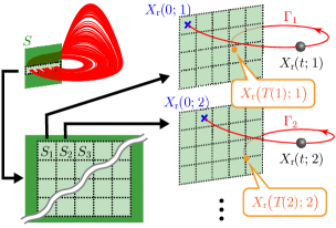
Figure 1: (Color online) Construction of $\left\{S_{i}\right\}$ and $\left\{\Gamma_{i}\right\}$.

Suppose that in an open neighborhood $U$ of the attractor $A$, there exists a change of coordinates

$$\begin{array}[]{ccc}U&\xrightarrow{\hskip 20.00003pt}&\mathbb{R}^{m-1}\times\left[0,\,2\mathord{\mathrm{\pi}}\right]\\[2.15277pt] \rotatebox{90.0}{$\in$}&&\rotatebox{90.0}{$\in$}\\[2.15277pt] X&\xmapsto{\hskip 20.00003pt}&\bigl{(}R(X),\,\phi(X)\bigr{)}\end{array}$$

such that $R$ is smooth in $U$, $\phi$ is continuous in $U$ and smooth in $U\setminus S$, $\phi(X)=0$ if and only if $X\in S\cap U$, and

$${\operatorname{d\!}\phi\bigl{(}X_{\text{r}}(t;\,i)\bigr{)}\over\operatorname{d\!}t}=\omega(i):={2\mathord{\mathrm{\pi}}\over T(i)}\quad\text{if\ \ {\hbox{0 < t < T(i)}}},$$ (2)

where the endpoints of the interval $\left[0,\,2\mathord{\mathrm{\pi}}\right]$ are identified with each other. Hereafter, we write $R\bigl{(}X(t)\bigr{)}$ and $\phi\bigl{(}X(t)\bigr{)}$ simply as $R(t)$ and $\phi(t)$. Although, in terms of the coordinates $\left(R,\,\phi\right)$, the system $\eqref{eq: free oscillator}$ can be formally expressed as

$$\dot{R}(t)=F_{R}\bigl{(}R(t),\,\phi(t)\bigr{)},\quad\dot{\phi}(t)=F_{\phi}\bigl{(}R(t),\,\phi(t)\bigr{)},$$ (3)

it is more convenient to rewrite the latter in a phase-oscillator-like form. Let $\mathscr{T}_{n}$ be the time of the $n$th return to $S$, and let $\mathscr{C}_{n}$ be the index of the cell in which the state of the system exists at $\mathscr{T}_{n}$. For $t\in\left(\mathscr{T}_{n},\,\mathscr{T}_{n+1}\right)$, the time evolution of $\phi$ can be expressed as follows:

$$\dot{\phi}(t)=\omega(\mathscr{C}_{n})+\rho\bigl{(}R(t),\,\phi(t)\bigr{)}.$$ (4)

When $t$ passes $\mathscr{T}_{n+1}$ (in other words, the next time the state returns to $S$), the evolution equation for $\phi$ is replaced with the equation corresponding to the next cell, $\mathscr{C}_{n+1}$. The condition $\eqref{eq: condition of uniform evolution}$ implies the condition

$$\rho\bigl{(}R_{\text{r}}(t-\mathscr{T}_{n};\,\mathscr{C}_{n}),\,\phi(t)\bigr{)}=0,$$ (5)

where $R_{\text{r}}(t;\,i):=R\bigl{(}X_{\text{r}}(t;\,i)\bigr{)}$.

Next, we consider the situation in which this oscillator is subject to a weak perturbation, $\varepsilon p(t)$, and the system is governed by the equation

$$\dot{X}(t)=F\bigl{(}X(t)\bigr{)}+\varepsilon p(t).$$

In this situation, the extent to which the time evolutions of $R$ and $\phi$ are perturbed depends on sensitivity functions. Explicitly, these time evolutions are described by the following:

$$\dot{R}(t)={} F_{R}\bigl{(}R(t),\,\phi(t)\bigr{)}+\varepsilon\left.{\partial R(X)\over\partial X}\right\rvert_{X=X(t)}p(t),$$ (6)

$$\dot{\phi}(t)={} \omega(\mathscr{C}_{n})+\rho\bigl{(}R(t),\,\phi(t)\bigr{)}$$

$${}+\varepsilon\left.\operatorname{grad}_{X}\phi(X)\right\rvert_{X=X(t)}\cdot p(t).$$ (7)

Let $\delta R(t)$ represent the deviation of $R(t)$ from its value on the representative trajectory; i.e., $\delta R(t):=R(t)-R_{\text{r}}(t-\mathscr{T}_{n};\,\mathscr{C}_{n})$ for $t\in\left(\mathscr{T}_{n},\,\mathscr{T}_{n+1}\right]$. Here, we assume that the surface of section, $S$, is partitioned so finely that $\left\lVert{\delta R(t)}\right\rVert$ can be regarded as a small quantity of $\operatorname{\mathcal{O}}(\varepsilon)$ until the next return to $S$. Ignoring terms of second and higher order in $\varepsilon$ and using the condition $\eqref{eq: rho on representative trajectory}$, we can rewrite Eqs. $\eqref{eq: perturbed evolution of amplitude}$ and $\eqref{eq: perturbed evolution of phase}$ as

$$\delta\dot{R}(t)={} \left.{\partial F_{R}\over\partial R}\right\rvert_{\vbox{\Let@\restore@math@cr\default@tag\halign{\hfil$\m@th\scriptstyle#$&$\m@th\scriptstyle{}#$\cr R&=R_{\text{r}}(t-\mathscr{T}_{n};\,\mathscr{C}_{n})\\ \phi&=\omega(\mathscr{C}_{n})\left(t-\mathscr{T}_{n}\right)\crcr}}}\delta R(t)$$ (10)

$${}+\varepsilon\left.{\partial R\over\partial X}\right\rvert_{X=X_{\text{r}}(t-\mathscr{T}_{n};\,\mathscr{C}_{n})}p(t),$$ (11)

$$\dot{\phi}(t)={} \omega\bigl{(}\mathscr{C}_{n}\bigr{)}+\left.\operatorname{grad}_{R}\rho(R,\,\phi)\right\rvert_{\vbox{\Let@\restore@math@cr\default@tag\halign{\hfil$\m@th\scriptstyle#$&$\m@th\scriptstyle{}#$\cr R&=R_{\text{r}}(t-\mathscr{T}_{n};\,\mathscr{C}_{n})\\ \phi&=\omega(\mathscr{C}_{n})\left(t-\mathscr{T}_{n}\right)\crcr}}}\cdot\delta R(t)$$ (14)

$${}+\varepsilon\zeta\bigl{(}\omega(\mathscr{C}_{n})\left(t-\mathscr{T}_{n}\right);\,\mathscr{C}_{n}\bigr{)}\cdot p(t),$$ (15)

where

$$\zeta(\phi;\,i) :=\left.\operatorname{grad}_{X}\phi(X)\right\rvert_{X=X_{\text{r}}[\phi/\omega(i);\,i]}.$$

Define $\delta R_{n}:=\lim_{t\downarrow\mathscr{T}_{n}}\delta R(t)=R_{n}-R_{\text{r}}(0;\,\mathscr{C}_{n})$, where $R_{n}:=R(\mathscr{T}_{n})$. Then for $t\in\left(\mathscr{T}_{n},\,\mathscr{T}_{n+1}\right]$, the differential equation $\eqref{eq: neglect small terms of perturbed system - amplitude}$ has the solution

$$\delta R(t)=\Phi(t-\mathscr{T}_{n};\,\mathscr{C}_{n})\left[\delta R_{n}\vphantom{+\varepsilon\int_{\mathscr{T}_{n}}^{t}\Upsilon(s-\mathscr{T}_{n};\,\mathscr{C}_{n})p(s)\operatorname{d\!}s}\right.\\ \left.\vphantom{\delta R_{n}}+\varepsilon\int_{\mathscr{T}_{n}}^{t}\Upsilon(s-\mathscr{T}_{n};\,\mathscr{C}_{n})p(s)\operatorname{d\!}s\right],$$ (16)

where $\Phi(t;\,i)$ is the fundamental matrix of the homogeneous equation

$$\delta\dot{R}(t)=\left.{\partial F_{R}\over\partial R}\right\rvert_{\vbox{\Let@\restore@math@cr\default@tag\halign{\hfil$\m@th\scriptstyle#$&$\m@th\scriptstyle{}#$\cr R&=R_{\text{r}}(t;\,i)\\ \phi&= \omega(i) t\crcr}}}\delta R(t)$$

whose value at the initial time, $\Phi(0;\,i)$, is the identity matrix, and

$$\Upsilon(t;\,i):=\Phi^{-1}(t;\,i)\left.{\partial R\over\partial X}\right\rvert_{X=X_{\text{r}}(t;\,i)}.$$

From Eq. $\eqref{eq: R-deviation from representative trajectory}$, we obtain the recurrence equation

$$R_{n+1} {}\simeq{} R_{\text{r}}\bigl{(}T(\mathscr{C}_{n});\,\mathscr{C}_{n}\bigr{)}+\Phi\bigl{(}T(\mathscr{C}_{n});\,\mathscr{C}_{n}\bigr{)}\left[\delta R_{n}\vphantom{+\varepsilon\int_{\mathscr{T}_{n}}^{\mathscr{T}_{n+1}}\Upsilon(t-\mathscr{T}_{n};\,\mathscr{C}_{n})p(t)\operatorname{d\!}t}\right.\quad$$

$$\left.\vphantom{\delta R_{n}}+\varepsilon\int_{\mathscr{T}_{n}}^{\mathscr{T}_{n+1}}\Upsilon(t-\mathscr{T}_{n};\,\mathscr{C}_{n})p(t)\operatorname{d\!}t\right]$$ . (17)

The second term on the right-hand side of Eq. $\eqref{eq: neglect small terms of perturbed system - phase}$ represents the deviation of the frequency from its value on the representative trajectory, which is caused by $\delta R(t)$. Now, assume that the surface of section is selected to be one for which the variation in the return time is very small. Specifically, we assume that this variation is sufficiently small that the second term on the right-hand side of Eq. $\eqref{eq: neglect small terms of perturbed system - phase}$ is much smaller than the third term. Ignoring this small term, Eq. $\eqref{eq: neglect small terms of perturbed system - phase}$ can be rewritten as

$$\dot{\phi}(t)=\omega(\mathscr{C}_{n})+\varepsilon\zeta\bigl{(}\phi(t);\,\mathscr{C}_{n}\bigr{)}\cdot p(t).$$ (18)

Equation $\eqref{eq: reduced phase equation (neglecting nonuniformity of frequency)}$ has the same form as the phase oscillator model, except for the $\mathscr{C}_{n}$-dependence. To remove the $\mathscr{C}_{n}$-dependence from Eq. $\eqref{eq: reduced phase equation (neglecting nonuniformity of frequency)}$, a bit more consideration is necessary. For simplicity, let us restrict the class of perturbations to periodic driving functions. With a weak periodic driving function $\varepsilon\tilde{p}(\theta)$ whose angular frequency, $\Omega$, is close to the average frequency of the unperturbed system $\eqref{eq: free oscillator}$, the time evolution of the phase difference, $\psi(t):=\phi(t)-\Omega t$, will be much slower than that of $R(t)$. In this case, it is reasonable to regard $\psi$ as a constant on the time scale of the $R$-dynamics. This allows us to reduce Eq. $\eqref{eq: map dynamics}$ to the map

$$R_{n+1}\simeq{} R_{\text{r}}\bigl{(}T(\mathscr{C}_{n});\,\mathscr{C}_{n}\bigr{)}$$

$${}+\Phi\bigl{(}T(\mathscr{C}_{n});\,\mathscr{C}_{n}\bigr{)}\left[\delta R_{n}+\varepsilon H(\mathscr{C}_{n},\,\psi)\right],$$ (19)

where $H(i,\,\psi)$ denotes the averaged effect of the periodic driving:

$$H(i,\,\psi)={1\over\omega(i)}\int_{0}^{2\mathord{\mathrm{\pi}}}\Upsilon\mathopen{}\left[{\phi\over\omega(i)};\,i\right]\mathclose{}\tilde{p}(\phi-\psi)\operatorname{d\!}\phi.$$

The chaotic behavior of the system is encapsulated in the map $\eqref{eq: reduced map dynamics}$. Iteration of Eq. $\eqref{eq: reduced map dynamics}$ produces the (conditional) natural measure $\mu_{i}(\psi;\,\varepsilon)$ [29, *blank2003multicomponent], the probability of visiting the cell $S_{i}$ under the condition that the phase difference is equal to $\psi$. Here, we ignore the small fluctuations in the actual phase difference $\psi(t)$ produced by the slight differences in $\omega(i)$ among the representative trajectories, and focus on the drift component of $\psi(t)$. Inside and near the synchronization region, the time scale characterizing the evolution of this drift component will be much longer than that characterizing the convergence of the relative frequency distribution of $S_{i}$ to the natural measure, $\mu_{i}$. Averaging the $\psi$-dynamics with respect to $\mu_{i}$, we obtain from Eq. $\eqref{eq: reduced phase equation (neglecting nonuniformity of frequency)}$ flow described by

$$\dot{\psi}(t)=\delta\omega\bigl{(}\psi(t);\,\varepsilon\bigr{)}+\varepsilon G\bigl{(}\psi(t);\,\varepsilon\bigr{)},$$ (20)

where

$$\left.\begin{gathered}\delta\omega(\psi;\,\varepsilon):=\overline{\omega}(\psi;\,\varepsilon)-\Omega,\quad\overline{\omega}(\psi;\,\varepsilon):={2\mathord{\mathrm{\pi}}\over\overline{T}(\psi;\,\varepsilon)},\\ \overline{T}(\psi;\,\varepsilon):=\sum_{i}\mu_{i}(\psi;\,\varepsilon)T(i),\\ G(\psi;\,\varepsilon):={1\over 2\mathord{\mathrm{\pi}}}\int_{0}^{2\mathord{\mathrm{\pi}}}\overline{\zeta}(\phi,\,\psi;\,\varepsilon)\cdot\tilde{p}(\phi-\psi)\operatorname{d\!}\phi,\\ \overline{\zeta}(\phi,\,\psi;\,\varepsilon):=\sum_{i}\mu_{i}(\psi;\,\varepsilon){T(i)\over\overline{T}(\psi;\,\varepsilon)}\zeta(\phi;\,i).\end{gathered}\,\right\}$$ (21)

This averaging may not be valid in a rigorous sense, because of the singularity of $\mu_{i}$ as a function of $\psi$. However, it can provide a rough approximation of the original system, as demonstrated in the following section. Note that the flow described by Eq. $\eqref{eq: flow dynamics}$ does not involve $\mathscr{C}_{n}$.

Several phase equations of the same form as Eq. $\eqref{eq: reduced phase equation (neglecting nonuniformity of frequency)}$ have been presented in previous studies (e.g., Ref. [21]). Here we have derived a reduced version of this description by separating the fast and slow dynamics (i.e., the dynamics of $R$ and $\psi$, respectively). This new description allows us to analyze the behavior of $R$ separately from the phase dynamics. [Note that $\psi$ in Eq. $\eqref{eq: reduced map dynamics}$ is a constant parameter whose value can be set independently of the state $\psi(t)$ of the flow $\eqref{eq: flow dynamics}$.] For this reason, it should be helpful in elucidating how the phase dynamics are affected by a change in the chaotic behavior of the non-phase variables.

What does the existence of the flow described by Eq. $\eqref{eq: flow dynamics}$ indicate? Note that Eq. $\eqref{eq: flow dynamics}$ can be viewed as an averaged equation derived from the phase oscillator

$$\dot{\phi}(t)=\overline{\omega}(\psi;\,\varepsilon)+\varepsilon\overline{\zeta}\bigl{(}\phi(t),\,\psi;\,\varepsilon\bigr{)}\cdot\tilde{p}(\Omega t),$$ (22)

which is adjusted by the map $\eqref{eq: reduced map dynamics}$ in the sense that $\overline{\omega}$ and $\overline{\zeta}$ depend on $\mu_{i}$ via Eqs. $\eqref{eq: adjuster}$. In other words, the rhythm dynamics of chaotic oscillators are described as a map-adjusted phase oscillator (MAPO). The existence of the flow described by Eq. $\eqref{eq: flow dynamics}$ therefore indicates that the MAPO $\eqref{eq: underlying phase oscillator}$ with the map $\eqref{eq: reduced map dynamics}$ determines the rhythmic properties (such as the average frequency) of the original chaotic oscillator, as illustrated in Fig. 2.

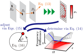
Figure 2: (Color online) Representation using the map-adjusted phase oscillator (MAPO) model depicting how the rhythmic properties of the chaotic oscillator are determined.

III Numerical Examples

In this section, we demonstrate the validity of the description proposed here through consideration of numerical examples.

III.1 The Rössler oscillator

As a first example, we consider the following Rössler oscillator [31] driven by a weak sinusoidal perturbation:

$$\begin{gathered}\dot{x}=-y-z+\varepsilon\sin\Omega t,\\ \dot{y}=x+ay,\quad\dot{z}=b+z\left(x-c\right),\end{gathered}$$ (23)

with the parameter values $a=0.2$, $b=0.2$, and $c=5.7$. Does the MAPO model consisting of Eqs. $\eqref{eq: reduced map dynamics}$ and $\eqref{eq: underlying phase oscillator}$ accurately produce the Arnold tongue for this system? The Arnold tongue can be constructed using the MAPO model by calculating the range of $\Omega$ in which there exists at least one value of $\psi$ satisfying the conditions

$$f_{\varepsilon}(\psi)=0\quad\text{and}\quad{\operatorname{d\!}f_{\varepsilon}\over\operatorname{d\!}\psi}(\psi)<0,$$ (24)

where $f_{\varepsilon}(\psi)$ denotes the right-hand side of Eq. $\eqref{eq: flow dynamics}$—i.e.,

$$f_{\varepsilon}(\psi)=\delta\omega(\psi;\,\varepsilon)+\varepsilon G(\psi;\,\varepsilon).$$

(For chaotic systems, averaged quantities, such as $\delta\omega$ and $G$, can be non-differentiable [32, *keller2008continuity, *baladi2014linear]. For this reason, in general, more careful consideration is needed.) To obtain $\delta\omega$ and $G$, we adopt the surface of section depicted in Fig. LABEL:fig:_demonstration_on_Rossler_oscillator_-_optimal_isophase, which is one of the optimal isophases (constructed using the method introduced in Ref. [28]) of the unperturbed system. With this surface of section, the variation in the return time [see Fig. LABEL:fig:_demonstration_on_Rossler_oscillator_-_return_time_distribution] is sufficiently small that Eq. $\eqref{eq: reduced phase equation (neglecting nonuniformity of frequency)}$ provides an accurate approximation of Eq. $\eqref{eq: neglect small terms of perturbed system - phase}$. Using numerical simulations, we can easily evaluate $T(i)$, $R_{\text{r}}\bigl{(}T(i);\,i\bigr{)}$, $\Phi\bigl{(}T(i);\,i\bigr{)}$, $\Upsilon(t;\,i)$, and $\zeta(\phi;\,i)$. This allows us to calculate $\delta\omega$ and $G$ defined in Eqs. $\eqref{eq: adjuster}$. With this treatment, the MAPO model produces the Arnold tongue depicted in Fig. LABEL:fig:_demonstration_on_Rossler_oscillator_-_tongue. Except in several isolated regions, the discrepancy between the form of the Arnold tongue derived from the MAPO model and that derived from the original model is small. The only significant discrepancy between the two consists of several horizontal spikes in the former [e.g., near $\left(\varepsilon,\,\Omega\right)=\left(0.021,\,1.077\right)$].

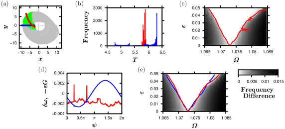
Figure 3: (Color online) Numerical results for the Rössler oscillator. LABEL:fig:_demonstration_on_Rossler_oscillator_-_optimal_isophase The trajectory (gray curve), the stroboscopic set [28] (green dots), and the adopted surface of section (red curve). The blue line segment represents a simpler surface of section ($x<0$, $y=0$). These surfaces of section yield the return time distributions plotted in LABEL:fig:_demonstration_on_Rossler_oscillator_-_return_time_distribution, where the red and blue histograms depict the distributions for the former and latter surfaces of section, respectively. LABEL:fig:_demonstration_on_Rossler_oscillator_-_tongue The difference between the frequencies of the periodic driving and the driven system observed in the full model. The red curve indicates the edge of the Arnold tongue derived from the MAPO model [i.e., the boundary of the $\left(\varepsilon,\,\Omega\right)$-region in which CPS occurs in the MAPO model]. LABEL:fig:_demonstration_on_Rossler_oscillator_-_characteristic_curves The instantaneous frequency difference $\delta\omega$ (red curve) and the coupling function $G$ (blue curve) at $\left(\varepsilon,\,\Omega\right)=\left(0.021,\,1.077\right)$. By preprocessing these quantities using a moving average filter, we obtained a more accurate approximation LABEL:fig:_demonstration_on_Rossler_oscillator_-_tongue_without_prickles. In this figure, for reference, the blue curve indicates the edge of the Arnold tongue obtained by using the other surface of section.

fig: demonstration on Rossler oscillator - optimal isophase fig: demonstration on Rossler oscillator - return time distribution fig: demonstration on Rossler oscillator - tongue fig: demonstration on Rossler oscillator - characteristic curves fig: demonstration on Rossler oscillator - tongue without prickles

To understand the appearance of the horizontal spikes, let us consider Fig. LABEL:fig:_demonstration_on_Rossler_oscillator_-_characteristic_curves, which plots the instantaneous frequency difference, $\delta\omega$, and the coupling function, $G$, on one of these spikes. The curves in this figure have jumps at several values of $\psi$. These jumps greatly extend the range of $\Omega$ in which there exists at least one value of $\psi$ satisfying the conditions $\eqref{eq: conditions of stable fixed point}$. This leads to the emergence of the spike. Closer investigation reveals that these jumps correspond to the values of $\psi$ at which narrow periodic windows appear in the $R$-dynamics $\eqref{eq: reduced map dynamics}$. The spikes reflect these large changes occurring in narrow parameter ranges.

The spikes are not observed in the Arnold tongue derived from the full model. This is because, in the full model, the phase difference $\psi$ fluctuates slightly on the time scale of the $R$-dynamics, and consequently $R$ does not remain confined to these narrow windows. This observation suggests that the fast fluctuations in $\psi$ play a key role in smoothing the frequency change.

To produce an effect similar to that caused by the fast fluctuations in $\psi$, we can utilize a moving average filter. By applying this filter to $\delta\omega$ and $G$, we can adjust the MAPO model so that it provides a more accurate approximation [see Fig. LABEL:fig:_demonstration_on_Rossler_oscillator_-_tongue_without_prickles].

The remaining slight difference between the Arnold tongues obtained from the full model and the MAPO model can be attributed to the anomalous enhancement of the diffusion coefficient discussed in Ref. [35]. This enhancement occurs near the point at which CPS breaks down and weakens the system’s periodicity in that region. Because the MAPO model is constructed assuming strong periodicity of the system, as this periodicity weakens, the discrepancy between the forms of the Arnold tongues derived from the full model and the MAPO model increases. However, as long as it is not too large, the error inherent in the form derived from the MAPO model does not prevent us from obtaining an accurate understanding of the global structure of the tongue, because this error is localized in the region near the point at which CPS breaks down.

III.2 The Lorenz oscillator

As a second example, we consider the following Lorenz oscillator [36] driven by a weak sinusoidal perturbation:

$$\label{eq:forcedLorenzequation}\begin{gathered}\dot{x}=\sigma\left(y-x\right)+\varepsilon\sin\Omega t,\\ \dot{y}=x\left(\rho-z\right)-y,\quad\dot{z}=xy-\beta z,\end{gathered}$$ (25)

with the parameter values $\sigma=10$, $\beta=8/3$, and $\rho=210$ [37]. We use the flat surface depicted in Fig. LABEL:fig:_demonstration_on_Lorenz_oscillator_-_trajectory_and_isophase as the surface of section. Although this surface was not determined through a careful optimization procedure, with it, the variation of the return time is indeed small, varying by only approximately $\pm 2\%$ [see Fig. LABEL:fig:_demonstration_on_Lorenz_oscillator_-_return_time_distribution]. (This is of similar magnitude to the variation observed in our investigation of the Rössler oscillator, discussed above, in which we used an optimal isophase.) With this small variation, the form of the Arnold tongue derived from the MAPO model in this case again deviates only slightly from that derived from the full model, as shown in Fig. LABEL:fig:_demonstration_on_Lorenz_oscillator_-_tongue.

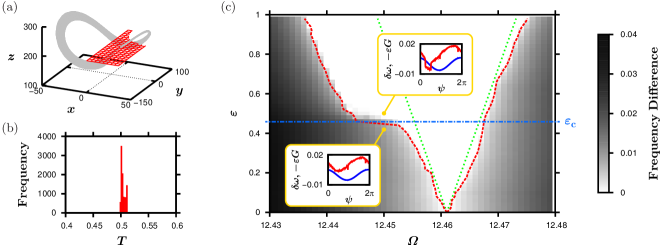
Figure 4: fig: demonstration on Lorenz oscillator(Color online) Numerical results for the Lorenz oscillator. LABEL:fig:_demonstration_on_Lorenz_oscillator_-_trajectory_and_isophase The trajectory (gray curve) and the adopted surface of section (red mesh surface). This surface of section yields the return time distribution plotted in LABEL:fig:_demonstration_on_Lorenz_oscillator_-_return_time_distribution. LABEL:fig:_demonstration_on_Lorenz_oscillator_-_tongue The difference between the frequencies of the periodic driving and the driven system observed in the full model. The dashed red curve indicates the edge of the Arnold tongue obtained from the MAPO model using the smoothed $\delta\omega$ and $G$. For reference, the edge of the tongue obtained by ignoring the perturbation dependence of the non-phase variables [i.e., by using $\delta\omega(\psi;\,0)$ and $G(\psi;\,0)$ instead of $\delta\omega(\psi;\,\varepsilon)$ and $G(\psi;\,\varepsilon)$] is indicated by the dotted green curve. The insets present representative examples of $\delta\omega$ (red curve) and $-\varepsilon G$ (blue curve) calculated in the regions above and below $\varepsilon=\varepsilon_{\text{c}}$, where $\varepsilon_{\text{c}}\approx 0.46$ is the value of $\varepsilon$ at which the Arnold tongue for the Lorenz oscillator exhibits an abrupt extension along the $\Omega$-axis. The crossing of $\delta\omega$ and $-\varepsilon G$ indicates that CPS occurs at the values of $\varepsilon$ and $\Omega$ used to plot their curves.

fig: demonstration on Lorenz oscillator - trajectory and isophase fig: demonstration on Lorenz oscillator - return time distribution fig: demonstration on Lorenz oscillator - tongue

The Arnold tongue for the Lorenz oscillator $\eqref{eq: forced Lorenz equation}$ exhibits an abrupt extension along the $\Omega$-axis at $\varepsilon=\varepsilon_{\text{c}}\approx 0.46$. This extension, like the spikes in the case of the Rössler oscillator, also reflects the appearance of periodic windows in the $R$-dynamics. The difference between the present situation and that for the Rössler oscillator is that in the present situation, the periodic windows are so wide that despite the fluctuations of $\psi$, $R$ remains confined to these windows for some time, and hence these windows have a strong effect even on the behavior of the full model. (Indeed, the Lorenz oscillator exhibits periodic behavior in part of the region above $\varepsilon=\varepsilon_{\text{c}}$, as reported in Ref. [37].) Note that the MAPO model accurately approximates the frequency in the regions both above and below $\varepsilon=\varepsilon_{\text{c}}$. This indicates that the MAPO model properly inherits the perturbation dependence of the non-phase variables from the full model. This inheritance results from the fact that $\overline{\omega}$ and $\overline{\zeta}$ in the phase oscillator $\eqref{eq: underlying phase oscillator}$ depend on the natural measure $\mu_{i}$; when the periodic driving triggers a qualitative change in the behavior of $R$, this change leads to large changes in $\mu_{i}$, and thus in the characteristics of the phase oscillator $\eqref{eq: underlying phase oscillator}$ [see the insets of Fig. LABEL:fig:_demonstration_on_Lorenz_oscillator_-_tongue]. In this way, the MAPO model successfully incorporates the dynamics of the non-phase variables existing in the system.

IV Conclusion

sec: Conclusion In summary, we have proposed the MAPO model as a framework for the study of CPS. This model consists of a chaotic map describing the evolution of the non-phase variables and a phase oscillator adjusted in accordance with the natural measure of the map, as illustrated in Fig. 2. This map, as well as the phase oscillator, depends on the perturbation applied to the original chaotic oscillator. Accordingly, the MAPO model allows us to examine how the perturbation induces a qualitative change in the behavior of the non-phase variables and alters the rhythmic properties of the chaotic oscillator.

In general, the Arnold tongues of chaotic oscillators may have distorted shapes different from the triangular shape exhibited by the tongues of limit-cycle oscillators. The origin of this distortion is clarified through analysis of the MAPO model, as demonstrated in Sec. III. In this way, the MAPO model helps us to understand the complicated nature of CPS.

Unlike conventional phase descriptions, the proposed phase description does not reduce the number of degrees of freedom of the model, because we need to iterate the $\left(m-1\right)$-dimensional map $\eqref{eq: reduced map dynamics}$ to generate the natural measure $\mu_{i}$. (Recall that $m$ denotes the number of degrees of freedom of the full model.) Nevertheless, the MAPO model has the advantage that in comparison to the full model, it provides a concise description of the rhythm dynamics, and for this reason, it clearly elucidates how the rhythmic properties of the chaotic oscillator are determined, as we now describe. First, the chaotic map $\eqref{eq: reduced map dynamics}$ describing the non-phase dynamics generates an orbit on the surface of section, which provides the natural measure $\mu_{i}$ under the perturbation. Next, this natural measure determines the properties of the phase oscillator $\eqref{eq: underlying phase oscillator}$ via Eq. $\eqref{eq: adjuster}$. Finally, the averaged equation $\eqref{eq: flow dynamics}$ derived from this phase oscillator determines the long-term rhythmic properties of the chaotic oscillator. For most chaotic oscillators, such a clear interpretation cannot be extracted from the full models. In addition, the MAPO model has the practical advantage that with it, we can obtain the Arnold tongue with a very short computation time, because even the most time-consuming step consists merely of the iteration of the map $\eqref{eq: reduced map dynamics}$ to generate the natural measure $\mu_{i}$. In this regard, it is important to note that we do not need to recalculate $T(i)$, $R_{\text{r}}\bigl{(}T(i);\,i\bigr{)}$, $\Phi\bigl{(}T(i);\,i\bigr{)}$, $\Upsilon(t;\,i)$, and $\zeta(\phi;\,i)$ every time the values of the parameters of the periodic driving are changed, because these functions are independent of the amplitude, frequency, and functional form of the periodic driving.

Although in this paper we have restricted the class of perturbations to external driving functions, preliminary results suggest that the rhythm dynamics of mutually interacting chaotic oscillators also can be described with the MAPO model. Further analysis of this point will be conducted in the near future.