Maximum of the characteristic polynomial of the Ginibre ensemble

Abstract

We compute the leading asymptotics for the maximum of the (centered) logarithm of the absolute value of the characteristic polynomial, denoted $\Psi_{N}$, of the Ginibre ensemble as the dimension of the random matrix $N$ tends to $+\infty$. The method relies on the log-correlated structure of the field $\Psi_{N}$ and we obtain the lower–bound for the maximum by constructing a family of Gaussian multiplicative chaos measures associated with certain regularization of $\Psi_{N}$ at small mesoscopic scales. We also obtain the leading asymptotics for the dimensions of the sets of thick points and verify that they are consistent with the predictions coming from the Gaussian Free Field. A key technical input is the approach from [4] to derive the necessary asymptotics, as well as the results from [60].

1 Introduction and main results

The Ginibre ensemble is the canonical example of a non–normal random matrix. It consists of a $N\times N$ matrix filled with independent complex Gaussian random variables of variance $1/N$, [31]. It is well–known that the eigenvalues $(\lambda_{1},\dots,\lambda_{N})$ of a Ginibre matrix are asymptotically uniformly distributed inside the unit disk $\mathbb{D}=\{z\in\mathbb{C}:|z|<1\}$ in the complex plane – this is known as the circular law [10, 16]. The Ginibre eigenvalues have the same law as the particles in a one component two–dimensional Coulomb gas confined by the potential $Q(x)=|x|^{2}/2$ at a specific temperature, see [56]. That is, the joint law of the eigenvalues is given by $\mathrm{d}\mathds{P}_{N}\propto e^{-\mathrm{H}_{N}(x)}{\textstyle\prod_{j=1}^{N}}\mathrm{d}^{2}x_{j}$ where the energy of a configuration $x\in\mathds{C}^{N}$ is

$$\mathrm{H}_{N}(x):=\sum_{\begin{subarray}{c}j,k=1,\dots,N\\ j\neq k\end{subarray}}\log|x_{j}-x_{k}|^{-1}+2N\sum_{j=1,\dots,N}Q(x_{j}),$$ (1.1)

and $\mathrm{d}^{2}x$ denotes the Lebesgue measure on $\mathds{C}$. Moreover, these eigenvalues form a determinantal point process on $\mathds{C}$ with a correlation kernel

$$K_{N}(x,z)={\textstyle\sum_{j=0}^{N-1}}\frac{x^{j}\overline{z}^{j}}{j!}N^{j+1}e^{-N|x|^{2}/2-N|z|^{2}/2}.$$ (1.2)

This means that all the correlation functions (or marginals $\mathds{P}_{N,n}$) of this point process are given by

$$\mathds{P}_{N,n}[\mathrm{d}x_{1},\cdots,\mathrm{d}x_{n}]=\frac{1}{(N)_{n}}\det\big{[}K_{N}(x_{i},x_{j})\big{]}_{i,j=1}^{n}\tfrac{\mathrm{d}^{2}x_{1}}{\pi}\cdots\tfrac{\mathrm{d}^{2}x_{n}}{\pi},\qquad\text{for }n=1,\dots,N,$$ (1.3)

where $(N)_{n}=N(N-1)\cdots(N-n+1)$. We refer to [33, Chapter 4] for an introduction to determinantal processes and to [33, Theorem 4.3.10] for a derivation of the Ginibre correlation kernel.

In this article we are interested in the asymptotics of the modulus of the characteristic polynomial $z\in\mathds{C}\mapsto\prod_{j=1}^{N}|z-\lambda_{j}|$ of the Ginibre ensemble and in particular on the maximum size of its fluctuations. Before stating our main result, we need to review some basic properties of the Ginibre eigenvalues process.

First, it follows from a classical result in potential theory that the equilibrium measure which describes the limit of the empirical measure $\frac{1}{N}\sum_{j=1}^{N}\delta_{\lambda_{j}}$ is indeed the circular law: $\sigma(\mathrm{d}x)=\frac{1}{\pi}\mathds{1}_{\mathds{D}}\mathrm{d}^{2}x$, see [56, Section 3.2]. Let $(x)_{+}=x\vee 0$ for $x\in\mathds{R}$. This can be deduced from the fact that the logarithmic potential of the circular law

$$\varphi(z):=\int\log|z-x|\sigma(\mathrm{d}x)=(\log|z|)_{+}-\frac{(1-|z|^{2})_{+}}{2},$$ (1.4)

satisfies the condition

$$\varphi(z)=Q(z)-1/2\qquad\text{for all $z\in\mathds{D}$}.$$ (1.5)

Then, Rider–Viràg [53] showed that the fluctuations of the empirical measure of the Ginibre eigenvalues around the circular law are described by a Gaussian noise. This result was generalized to other ensembles of random matrices in [3, 4], as well as to two–dimensional Coulomb gases at an arbitrary positive temperature in [9, 46]. Let us define

$$\mathrm{X}(\mathrm{d}x):={\textstyle\sum_{j=1}^{N}\delta_{\lambda_{j}}}-N\sigma(\mathrm{d}x).$$ (1.6)

This measure describes the fluctuations of the Ginibre eigenvalues and, by [53, Theorem 1.1], for any function $f\in\mathscr{C}^{2}(\mathds{C})$ with at most exponential growth, we have as $N\to+\infty$,

$$\mathrm{X}(f)={\textstyle\sum_{j=1}^{N}f(\lambda_{j})}-N\int f(x)\sigma(\mathrm{d}x)\ \overset{\rm law}{\longrightarrow}\ \mathscr{N}\left(0,\Sigma^{2}(f)\right).$$ (1.7)

If $f$ has compact support inside the support of the equilibrium measure, then the asymptotic variance is given by

$$\Sigma^{2}(f)=\int\overline{\partial}f(x)\partial f(x)\sigma(\mathrm{d}x).$$ (1.8)

The object that we study in this article is the centered logarithm of the Ginibre characteristic polynomial:

$$\Psi_{N}(z):=\log\left({\textstyle\prod_{j=1}^{N}}|z-\lambda_{j}|\right)-N\varphi(z).$$ (1.9)

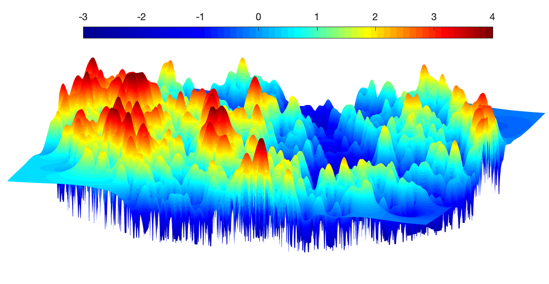
Figure 1: Sample of the logarithm of the absolute value of the Ginibre characteristic polynomial $\Psi_{N}(z)$ for $z\in\mathds{D}$ for a random matrix of dimension $N=3000$.

See Figure 1 below for a sample of the random function $\Psi_{N}(z)$. Note that it follows from the convergence of the empirical measure to the circular law that for any $z\in\mathds{C}$, we have in probability as $N\to+\infty$,

$$\frac{1}{N}\log\left({\textstyle\prod_{j=1}^{N}}|z-\lambda_{j}|\right)\to\varphi(z),$$

so that the second term on the RHS of (1.9) is necessary to have the field $\Psi_{N}$ asymptotically centered. In fact, it follows from the result of Webb–Wong [60] that $\mathds{E}_{N}[\Psi_{N}(z)]\to 1/4$ for all $z\in\mathds{D}$ as $N\to+\infty$. Moreover, if we interpret $\Psi_{N}$ as a random generalized function, then the central limit theorem (1.7) implies that $\Psi_{N}$ converges in distribution to the Gaussian free field (GFF) on $\mathds{D}$ with free boundary conditions, see [53, Corollary 1.2] and also [4, 58] for further details. Even though the GFF is a random distribution, it can be though of as a random surface which corresponds to the two–dimensional analogue of Brownian motion, [57]. The convergence result of Rider–Viràg indicates that we can think of the field $\Psi_{N}$ as an approximation of the GFF in $\mathds{D}$. The main feature of the GFF is that it is a log-correlated Gaussian process on $\mathds{C}$. This log-correlated structure is already visible for the absolute value of the Ginibre characteristic polynomial as it is possible to show that for any $z,x\in\mathds{D}$,

$$\mathds{E}_{N}\left[\Psi_{N}(z)\Psi_{N}(x)\right]=\frac{1}{2}\log\left(\sqrt{N}\wedge|x-z|^{-1}\right)+\mathcal{O}(1),$$ (1.10)

as $N\to+\infty$. By analogy with the GFF and other log-correlated fields, we can make the following prediction regarding the maximum of the field $\Psi_{N}$. We have as $N\to+\infty$,

$$\max_{z\in\mathds{D}}\Psi_{N}(z)=\frac{\log N}{\sqrt{2}}-\frac{3\log\log N}{4\sqrt{2}}+\xi_{N},$$ (1.11)

where the random variable $\xi_{N}$ is expected to converge in distribution. Analogous predictions have been made for other log-correlated fields associated with normal random matrices. For instance, Fyodorov–Keating [28] first conjectured the asymptotics of the maximum of the logarithm of the absolute value of the characteristic polynomial of the circular unitary ensemble (CUE), including the distribution of the error term and Fyodorov–Simm [30] made analogous prediction for the Gaussian Unitary Ensemble (GUE) .

The main goal of this article is to verify the leading order in the asymptotic expansion (1.11). More precisely, we prove the following result:

Theorem 1.1.

For any $0<r<1$ and any $\epsilon>0$, it holds

$$\lim_{N\to+\infty}\mathds{P}_{N}\left[\frac{1-\epsilon}{\sqrt{2}}\log N\leq\max_{|z|\leq r}\Psi_{N}(z)\leq\frac{1+\epsilon}{\sqrt{2}}\log N\right]=1.$$

It is worth pointing out that like many other asymptotic properties of the eigenvalues of random matrices, we expect the results of Theorem 1.1, as well as the prediction (1.11) modulo the limiting distribution of $\xi_{N}$, and Theorem 1.3 below to be universal. This means that these results should hold for other random normal matrix ensembles with a different confining potential $Q$ as well as for other non–Hermitian Wigner ensembles under reasonable assumptions on the entries of the random matrix. In the remainder of this section, we review the context and most relevant results related to Theorem 1.1, and we provide several motivations to study the characteristic polynomial of the Ginibre ensemble.

1.1 Comments on Theorem 1.1 and further results

The study of characteristic polynomials for different ensembles of random matrices is an interesting and active topic because of its connections to several problems in diverse areas of mathematics. In particular, there are the analogy between the logarithm of the absolute value of the characteristic polynomial of the CUE and the Riemann $\zeta$-function [38], as well as the connections with Toeplitz or Hankel determinant with Fisher–Hartwig symbols, e.g. [41, 24, 18, 19]. Of essential importance is also the connection between characteristic polynomial of random matrices, log-correlated fields and the theory of Gaussian multiplicative chaos [35, 28]. This connection has been used in several recent works to compute the asymptotics of the maximum of the logarithm of the characteristic polynomial for various ensembles of random matrices. For the CUE, a result analogous to Theorem 1.1 was first obtained by Arguin–Belius–Bourgade [5]. Then, the correction term was computed by Paquette–Zeitouni [49] and the counterpart of the conjecture (1.11) was established for the circular $\beta$-ensembles for general $\beta>0$ by Chhaibi–Madaule–Najnudel [20]. For the characteristic polynomial of the GUE, as well as other Hermitian unitary invariant ensembles, the law of large numbers for the maximum of the absolute value of the characteristic polynomial was obtained in [43]. Cook and Zeitouni [23] also obtained a law of large numbers for the maximum of the characteristic polynomial of a random permutation matrix, in which case their result does not match with the prediction from Gaussian log-correlated field because of arithmetic effects. These results rely on the log-correlated structure of characteristic polynomials and proceed by analogy with the case of branching random walk using a modified second moment method, [39]. This method has also been successful to compute the asymptotics of the Riemann $\zeta$-function in a random interval of the critical line, see [55, 47, 6, 32]. Further recent results on the deep connections between log-correlated fields, Gaussian multiplicative chaos and characteristic polynomials of $\beta$-ensembles can be found in [22, 21, 44] In particular, we prove in [22] the counterpart of Theorem 1.1 for the imaginary part of the characteristic polynomial of a large class of Hermitian unitary invariant ensembles and show that this implies optimal rigidity bounds for the eigenvalues. Likewise, by adapting the proof of the upper–bound in Theorem 1.1, we can obtain precise rigidity estimates for linear statistics of the Ginibre ensemble in the spirit of [8, Theorem 1.2] and [46, Theorem 2].

Theorem 1.2.

For any $0<r<1$ and $\kappa>0$, define

$$\mathscr{F}_{r,\kappa}:=\left\{f\in\mathscr{C}^{2}(\mathds{C}):\Delta f(z)=0\ \text{ for all }z\in\mathds{C}\setminus\mathds{D}_{r}\text{ and }\max_{\mathds{C}}|\Delta f|\leq N^{\kappa}\right\}.$$ (1.12)

For any $\eta>0$ (possibly depending on $N$ with $\eta\leq\frac{N}{\log N}$), there exists a constant $C_{r}>0$ such that

$$\mathds{P}_{N}\bigg{[}\sup\left\{|\mathrm{X}(f)|:f\in\mathscr{F}_{r,\kappa}\text{ and }\int_{\mathds{D}}|\Delta f(z)|\frac{\mathrm{d}^{2}z}{\pi}\leq 1\right\}\geq\eta\log N+1\bigg{]}\leq C_{r}N^{5/4+\kappa-\eta}.$$

We believe that Theorem 1.2 is of independent interest since it covers any smooth mesoscopic linear statistic at arbitrary small scales in a uniform way. This is to be compared to the local law of [17, Theorem 2.2] which is valid for general Wigner ensembles, but not with the (optimal) logarithmic bound for the fluctuations and without such uniformity in $f$. The proof of Theorem 1.2 is given in Section 3.2 and it relies on the basic observation that in the sense of distribution, the Laplacian of the field $\Psi_{N}$ is related to the empirical measure of the Ginibre ensemble suitably centered: $\Delta\Psi_{N}=2\pi N\left(\frac{1}{N}\sum_{j=1}^{N}\delta_{\lambda_{j}}-\frac{1}{\pi}\mathds{1}_{\mathds{D}}\right)$.

The proof of Theorem 1.1 consists of an upper–bound which is based on the subharmonicity of the logarithm of the absolute value of the Ginibre characteristic polynomial and the moments asymptotics from Webb–Wong [60] and of a lower–bound which exploits the log-correlated structure of the field $\Psi_{N}$. More precisely, by relying on the robust approach from [45], we obtain the lower–bound in Theorem 1.1 by constructing a family of subcritical Gaussian multiplicative chaos measures associated with certain mesoscopic regularization of the field $\Psi_{N}$ – see Theorem 2.2 below for further details. Gaussian multiplicative chaos (GMC) is a theory which goes back to Kahane [37] and it aims at encoding geometric features of a log-correlated field by means of a family of random measures. These GMC measures are defined by taking the exponential of a log-correlated field through a renormalization procedure. We refer the readers to Section 2.1 for a brief overview of the theory and to the review of Rhodes–Vargas [51] or the elegant and short article of Berestycki [11] for more comprehensive presentations. It is well–known that in the subcritical phase, these GMC measures live on the sets of so–called thick points of the underlying field, [51, Section 4]. By exploiting this connection, we obtain from our analysis the leading order of the measure of the sets of thick points of the characteristic polynomial for large $N$.

Theorem 1.3.

Let us define the set of $\beta$-thick points of the Ginibre characteristic polynomial:

$$\mathscr{T}_{N}^{\beta}(r):=\big{\{}x\in\overline{\mathds{D}_{r}}:\Psi_{N}(x)\geq\beta\log N\big{\}}$$ (1.13)

and let $|\mathscr{T}_{N}^{\beta}(r)|$ be its Lebesgue measure. For any $0<r<1$, any $0\leq\beta<1/\sqrt{2}$ and any small $\epsilon>0$, we have

$$\lim_{N\to+\infty}\mathds{P}_{N}\left[N^{-2\beta^{2}-\delta}\leq|\mathscr{T}_{N}^{\beta}(r)|\leq N^{-2\beta^{2}+\delta}\right]=1.$$ (1.14)

The proof of Theorem 1.3 will be given in Section 4 and the result has the following interpretation. By (1.9), the field $-\Psi_{N}$ corresponds to the (electrostatic) potential energy generated by the random charges $(\lambda_{1},\dots,\lambda_{N})$ and the negative uniform background $\sigma$. One may view $-\Psi_{N}$ as a complex energy landscape and the asymptotics (1.14) describe the multi–fractal spectrum of the level sets near the extreme local minima of this landscape. Moreover, as a consequence of Theorems 1.1 and 1.3, we obtain the leading order of the corresponding free energy, i.e. the logarithm of the partition function of the Gibbs measure $e^{\beta\Psi_{N}}$ for $\beta>0$. Namely, by adapting the proof of [5, Corollary 1.4], it holds for any $0<r<1$, in probability,

$$\lim_{N\to+\infty}\frac{1}{\beta\log N}\log\left(\int_{\mathds{D}_{r}}e^{\beta\Psi_{N}(z)}\frac{\mathrm{d}^{2}z}{\pi}\right)=\max_{\gamma\in[0,1/\sqrt{2}]}\Big{\{}\frac{1}{\beta}+\gamma-\frac{2}{\beta}\gamma^{2}\Big{\}}=\begin{cases}\displaystyle\frac{1}{\beta}+\frac{\beta}{8},&\beta\in[0,\sqrt{8}]\\ \displaystyle 1/\sqrt{2},&\beta>\sqrt{8}\end{cases}.$$ (1.15)

The fact that the free energy is constant and equal to ${\displaystyle\lim_{N\to+\infty}}\frac{\max_{\mathds{D}_{r}}\Psi_{N}}{\log N}$ in the supercritical regime $\beta>\sqrt{8}$ is called freezing. This property is typical for Gaussian log-correlated fields and our results rigorously establish that the Ginibre characteristic polynomial behave according to the Gaussian predictions which is a well–known heuristic in random matrix theory. Moreover, this freezing scenario is instrumental to predict the full asymptotic behavior (1.11) of the maximum of the field $\Psi_{N}$, including the law of the error term, see e.g. [27]. For an illustration of level sets of the random function and in particular of the geometry of thick points, see Figure 2.

Let us return to the connections between our results and the theory of Gaussian multiplicative chaos. The family of GMC measures associated to the GFF are called Liouville measures and they play a fundamental role in recent probabilistic constructions in the context of quantum gravity, imaginary geometries, as well as conformal field theory. We refer to the reviews [7, 52] for further references on these aspects of the theory. Thus, motivated by the result of Rider–Viràg, it is expected that a random measure whose density is given by a small power of the characteristic polynomial (see Figure 3 below) converges when suitably normalized:

$$\frac{\prod_{j=1}^{N}|z-\lambda_{j}|^{\gamma}}{\mathds{E}_{N}\left[\prod_{j=1}^{N}|z-\lambda_{j}|^{\gamma}\right]}\frac{\mathrm{d}^{2}z}{\pi}=\frac{e^{\gamma\Psi_{N}(z)}}{\mathds{E}_{N}\left[e^{\gamma\Psi_{N}(z)}\right]}\frac{\mathrm{d}^{2}z}{\pi}\ \overset{\rm law}{\longrightarrow}\ \mu_{\mathrm{G}}^{\gamma},$$ (1.16)

where $\mu_{\mathrm{G}}^{\gamma}$ is a Liouville measure with parameter $0<\gamma<\sqrt{8}$. Hence, this provides an interesting connection between the Ginibre ensemble of random matrices and random geometry. As we observed in [22, Section 3], this convergence result in the subcritical phase implies the lower–bound in Theorem 1.1. An important observation that we make in this paper is that it suffices to establish the convergence of $\frac{e^{\gamma\psi_{N}(z)}}{\mathds{E}_{N}\left[e^{\gamma\psi_{N}(z)}\right]}\frac{\mathrm{d}^{2}z}{\pi}$ to a GMC measure for a suitable regularization $\psi_{N}$ of the field $\Psi_{N}$ in order to capture the correct leading order asymptotics of its maximum and thick points. The main issues are to work with a regularization at an optimal mesoscopic scale $N^{-1/2+\alpha}$ for arbitrary small $\alpha>0$ and to be able to obtain the convergence in the whole subcritical phase. In particular, our result on GMC, Theorem 2.2, provides strong evidence that the prediction (1.16) holds.

It is an important and challenging problem to obtain (1.16) already in the subcritical phase. In particular, this requires to derive the asymptotics of joint moments of the characteristic polynomials. For a single $z\in\mathds{D}_{r}$, such asymptotics are obtained by Webb–Wong in [60] using Riemann–Hilbert techniques. Let us recall their main result which is also a key input in our method.

Theorem 1.4 ([60], Theorem 1.1).

For any fixed $0<r<1$, we have

$$\mathds{E}_{N}[e^{\gamma\Psi_{N}(z)}]=(1+o(1))\frac{(2\pi)^{\gamma/4}}{G(1+\gamma/2)}N^{\gamma^{2}/8},$$ (1.17)

where the error term is uniform for $\gamma$ in compact sets of $\{\gamma\in\mathds{C}:\Re\gamma>-2\}$ and $z\in\mathds{D}_{r}$.

Remark 1.5.

The asymptotics of the joint exponential moments of $\Psi_{N}$ remain conjectural, see e.g. [60, Section 1.2], except for even moments for which there are explicit formulae, see [1, 29, 26]. These formulae rely on the determinantal structure of the Ginibre ensemble: for any $n\in\mathbb{N}$, we have for any $z_{1},\dots,z_{n}\in\mathds{C}$ such that $z_{1}\neq\cdots\neq z_{n}$,

$$\mathds{E}_{N}\left[{\textstyle\prod_{i=1}^{n}\prod_{j=1}^{N}}|z_{i}-\lambda_{j}|^{2}\right]=\frac{\pi^{n}\prod_{k=N}^{N+n-1}k!}{N^{-Nn-\frac{n(n+1)}{2}}}\frac{\det_{n\times n}[K_{N+n}(z_{i},z_{j})]}{\prod_{1\leq i<j\leq n}|z_{i}-z_{j}|^{2}}e^{N\sum_{i=1}^{n}|z_{i}|^{2}},$$ (1.18)

where $K_{N+n}$ is the Ginibre kernel as in (1.2). Using the off–diagonal (Gaussian) decay of the Ginibre kernel, we can show that

$$\det_{n\times n}[K_{N+n}(z_{i},z_{j})]={\textstyle\prod_{k=1}^{n}}K_{N+n}(z_{i},z_{i})\left(1+\mathcal{O}(N^{-1})\right),$$

uniformly for all $\inf_{i\neq j}|z_{i}-z_{j}|\geq c\sqrt{\frac{\log N}{N}}$ if $c>0$ is a sufficiently large constant. If $|z_{i}|\leq c\sqrt{\frac{\log N}{N}}$, we also have $K_{N+n}(z_{i},z_{i})=\tfrac{N}{\pi}\left(1+\mathcal{O}(N^{-1})\right)$. Thus, by (1.5) and (1.9) we obtain that for any given $z_{1},\dots,z_{n}\in\mathds{D}$, such that $z_{1}\neq\cdots\neq z_{n}$,

$$\mathds{E}_{N}\big{[}{\textstyle\prod_{i=1}^{n}}e^{2\Psi_{N}(z_{i})}\big{]}=\left(\sqrt{2\pi N}\right)^{n}|\triangle(z_{1},\dots,z_{n})|^{-2}\left(1+\mathcal{O}(N^{-1})\right),$$ (1.19)

which matches exactly with the Fisher–Hartwig predictions from [60, Section 1.2] with $\gamma_{1}=\cdots=\gamma_{n}=2$. $\blacksquare$

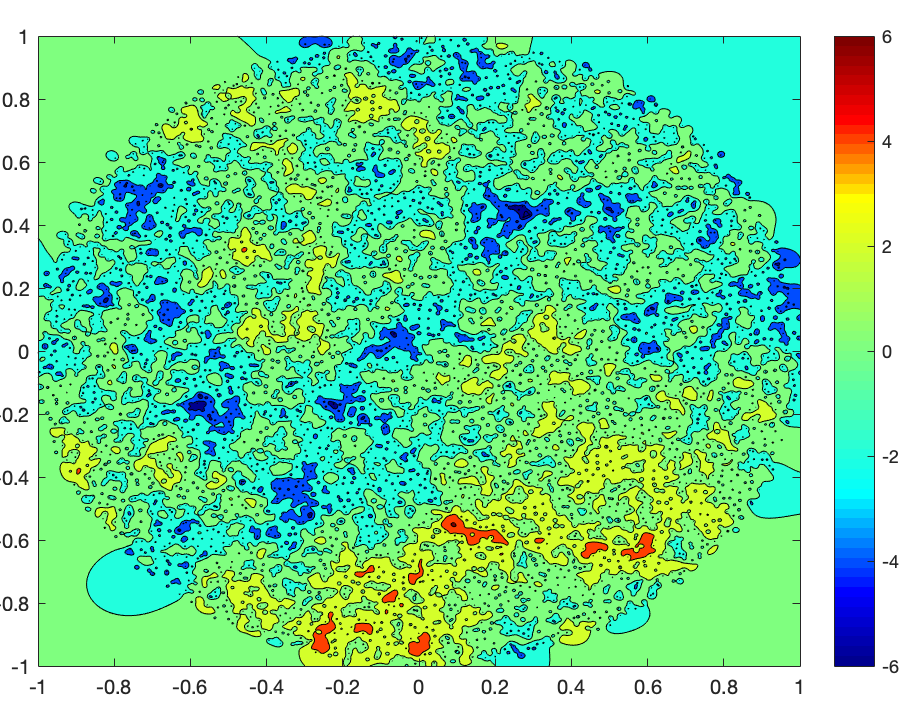
Figure 2: Level sets of the logarithm of the absolute value of the Ginibre characteristic polynomial $\Psi_{N}(z)$ for a random matrix of dimension $N=5000$.

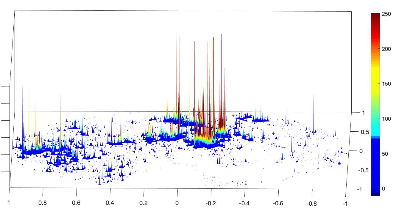
Figure 3: Sample of the (normalized) Ginibre characteristic polynomial $\frac{\prod_{j=1}^{N}|z-\lambda_{j}|}{\mathds{E}_{N}[\prod_{j=1}^{N}|z-\lambda_{j}|]}$ for a random matrix of dimension $N=3000$. This is an approximation of the Liouville measure $\mu_{G}^{\gamma}$ with (subcritical) parameter $\gamma=1$.

1.2 Outline of the article

The remainder of this article is devoted to the proof of Theorem 1.1. The result follows directly by combining the upper–bound of Proposition 3.1 and the lower–bound from Proposition 2.1. As we already emphasized the proof of the lower–bound follows from the connection with GMC theory and the details of the argument are reviewed in Section 2. In particular, it is important to obtain Gaussian asymptotics for the exponential moments of a mesoscopic regularization of the field $\Psi_{N}$, see Proposition 2.3. These asymptotics are obtained by using the method developed by Ameur–Hedenmalm–Makarov [4] which relies on Ward identity, also known as loop equation, and the determinantal structure of the Ginibre ensemble. Compared with the proof of the central limit theorem in [4], we face two significant extra technical challenges: we must consider a mesoscopic linear statistic coming from a test function which develops logarithmic singularities as $N\to+\infty$. This implies that we need a more precise approximation for the correlation kernel of the biased determinantal process. For these reasons, we give a detailed proof of Proposition 2.3 in Section 5 and Section 6. Our proof for the upper–bound is given in Section 3 and it relies on the subharmonicity of the logarithm of the absolute value of the Ginibre characteristic polynomial and the asymptotics from Theorem 1.4. In Section 3.2, we discuss an application to linear statistics of the Ginibre eigenvalues and give the proof of Theorem 1.2.

1.3 Acknowledgment

G.L. is supported by the University of Zurich Forschungskredit grant FK-17-112 and by the grant SNSF Ambizione S-71114-05-01. G.L. wishes to thank P. Bourgade for insightful discussions about the problem considered here and the referee for interesting comments which helped to improve the presentation of this article and for pointing out several references.

2 Proof of the lower–bound

Recall that $\Psi_{N}$ denotes the centered logarithm of the absolute value of the Ginibre characteristic polynomial, (1.9). The goal of this section is to obtained the following result:

Proposition 2.1.

For any $r>0$ and any $\delta>0$, we have

$$\lim_{N\to+\infty}\mathds{P}_{N}\left[\max_{|x|\leq r}\Psi_{N}(x)\geq\frac{1-\delta}{\sqrt{2}}\log N\right]=1.$$

Our strategy to prove Proposition 2.1 is to obtain an analogous lower–bound for a mesoscopic regularization of $\Psi_{N}$ which is also compactly supported inside $\mathds{D}$. Note that it is also enough to consider the maximum in a disk $\mathds{D}_{\epsilon_{0}}=\{x\in\mathds{C}:|x|\leq\epsilon_{0}\}$ for a small $\epsilon_{0}>0$. To construct such a regularization, let us fix $0<\epsilon_{0}\leq 1/4$ and a mollifier $\phi\in\mathscr{C}^{\infty}_{c}(\mathds{D}_{\epsilon_{0}})$ which is radial. For any $0<\epsilon<1$, we denote $\phi_{\epsilon}(\cdot)=\phi(\cdot/\epsilon)\epsilon^{-2}$ and to approximate the logarithm of the characteristic polynomial, we consider the test function

$$\psi_{\epsilon}(z):=\int\log|z-x|\phi_{\epsilon}(x)\mathrm{d}^{2}x.$$ (2.1)

We also denote $\psi=\psi_{1}$. For technical reason, it is simpler to work with test function compactly supported inside $\mathds{D}$ – which is not the case for $\psi_{\epsilon}$. However, this can be fixed by making the following modification: for any $z\in\mathds{D}_{\epsilon_{0}}$, we define

$$g_{N}^{z}(x):=\psi_{\epsilon}(x-z)-\psi(x-z),\qquad x\in\mathds{C}.$$ (2.2)

It is easy to see that the function $g_{N}^{z}$ is smooth and compactly supported inside $\mathds{D}(z,\epsilon_{0})$. Since we are interested in the regime where $\epsilon(N)\to 0$ as $N\to+\infty$, we emphasize that $g_{N}^{z}$ depends on the dimension $N\in\mathbb{N}$ of the matrix. Then, the random field $z\mapsto\mathrm{X}(g_{N}^{z})$ is related to the logarithm of the Ginibre characteristic polynomial as follows:

$$\mathrm{X}(g_{N}^{z})=\int\Psi_{N}(x)\phi_{\epsilon}(z+x)\mathrm{d}^{2}x-\int\Psi_{N}(x)\phi(z+x)\mathrm{d}^{2}x.$$ (2.3)

In particular, $z\mapsto\mathrm{X}(g_{N}^{z})$ is still an approximate log-correlated field. Indeed, according to (1.7), (1.8) and formula (2.8) below, we expect that as $N\to+\infty$

$$\mathds{E}_{N}\left[\mathrm{X}(g_{N}^{z})\mathrm{X}(g_{N}^{x})\right]=\frac{1}{2}\log\left(\epsilon(N)^{-1}\wedge|x-z|^{-1}\right)+\mathcal{O}(1).$$

This should be compared with formula (1.10).

2.1 Gaussian multiplicative chaos

Let $\mathrm{G}$ be the Gaussian free field (GFF) on $\mathds{D}$ with free boundary conditions. That is, $\mathrm{G}$ is a Gaussian process taking values in the space of Schwartz distributions with covariance kernel:

$$\mathds{E}\left[\mathrm{G}(x)\mathrm{G}(z)\right]=\frac{1}{2}\log|z-x|^{-1}.$$ (2.4)

Up to a factor of $1/\pi$, the RHS of (2.4) is the Green’s function for the Laplace operator $-\Delta$ on $\mathds{C}$. Because of the singularity of the kernel (2.4) on the diagonal, $\mathrm{G}$ is called a log-correlated field and it cannot be defined pointwise. In general, $\mathrm{G}$ is interpreted as a random distribution valued in a Sobolev space $H^{-\alpha}(\mathds{D})$ for any $\alpha>0$, [7]. In particular, for any mollifier $\phi$ as above and any $\epsilon>0$, we view

$$\mathrm{G}_{\epsilon}(z):=\int\mathrm{G}(x)\phi_{\epsilon}(z+x)\mathrm{d}^{2}x$$ (2.5)

as a regularization of $\mathrm{G}$.

The theory of Gaussian multiplicative chaos aims at defining the exponential of a log-correlated field. Since such a field is merely a random distribution, this is a non trivial problem. However, in the so-called subcritical phase, this can be done by a quite simple renormalization procedure. Namely, for $\gamma>0$, we define $\mu^{\gamma}_{\mathrm{G}}=:e^{\gamma\mathrm{G}}:$ as

$$\mu^{\gamma}_{\mathrm{G}}(\mathrm{d}x):=\lim_{\epsilon\to 0}\frac{e^{\gamma\mathrm{G}_{\epsilon}(x)}}{\mathds{E}[e^{\gamma\mathrm{G}_{\epsilon}(x)}]}\sigma(\mathrm{d}x).$$ (2.6)

It turns out that this limit exists almost surely as a random measure on $\mathds{D}$ and that it does not depend on the mollifier $\phi$ within a reasonable class. Moreover, in the case of the GFF normalized as in (2.4), it is a non trivial measure if and only if the parameter $0<\gamma<\sqrt{8}$ – this is called the subcritical phase, [54, 11, 7]. For general log-correlated field, the theory of GMC goes back to the work of Kahane [37] and in the case of the GFF, the construction $\mu^{\gamma}_{\mathrm{G}}$ was re-discovered by Duplantier–Sheffield [25] and Rhodes–Vargas [50] from different perspectives. In a sense, the random measure $\mu^{\gamma}_{\mathrm{G}}$ encodes the geometry of the GFF. For instance, the support of $\mu^{\gamma}_{\mathrm{G}}$ is a fractal set which is closely related to the concept of thick points, [34]. We will not discuss these issues here and refer instead to [7, 22] for further details. Let us just point out that the relationship between Theorem 2.2 and Corollary 2.4 below is based on such arguments.

For log-correlated fields which are only asymptotically Gaussian, especially those coming from random matrix theory such as the logarithm of the Ginibre characteristic polynomial $\Psi_{N}$, the theory of Gaussian multiplicative chaos has been developed in [59, 45]. The construction in [45] is inspired from the approach of Berestycki [11] and it has been recently applied to unitary random matrices in [48], as well as to Hermitian unitary invariant random matrices in [12, 22]. In this paper, we construct subcritical GMC measures coming from the regularization $\mathrm{X}(g_{N}^{z})$, (2.3), of the logarithm of the Ginibre characteristic polynomial at a scale $\epsilon=N^{-1/2+\alpha}$ for any small $\alpha>0$. This mesoscopic regularization makes it simpler to compute the leading asymptotics of the exponential moments of the field $\mathrm{X}(g_{N}^{z})$ – see Proposition 2.3 below. Then, using the main results from [45], it allows us to prove that the limit of the renormalized exponential $\mu^{\gamma}_{N}=:e^{\gamma\mathrm{X}(g_{N}^{z})}:$ exists for all $\gamma>0$ in the subcritical phase and that it is absolutely continuous with respect to the GMC measure $\mu^{\gamma}_{\mathrm{G}}$.

Theorem 2.2.

Recall that $0<\epsilon_{0}\leq 1/4$ is fixed. Let $\gamma>0$ and $g_{N}^{z}$ be as in (2.2) with $\epsilon=\epsilon(N)=N^{-1/2+\alpha}$ for a fixed $0<\alpha<1/2$. Let us define the random measure $\mu^{\gamma}_{N}$ on $\mathds{D}_{\epsilon_{0}}$ by

$$\mu^{\gamma}_{N}(\mathrm{d}z):=\frac{\exp\left(\gamma\mathrm{X}(g_{N}^{z})\right)}{\mathds{E}_{N}[\exp\left(\gamma\mathrm{X}(g_{N}^{z})\right)]}\sigma(\mathrm{d}z).$$

For any $0<\gamma<\gamma_{*}=\sqrt{8}$, the measure $\mu^{\gamma}_{N}$ converges in law as $N\to+\infty$ with respect to the weak topology toward a random measure $\mu^{\gamma}_{\infty}$ which has the same law, up to a deterministic constant, as $e^{\gamma\mathrm{G}_{1}(x)}\mu^{\gamma}_{\mathrm{G}}(\mathrm{d}x)$, where $\mathrm{G}_{1}$ is the smooth Gaussian process obtained from $\mathrm{G}$ as in (2.5) with $\epsilon=1$ and $\mu^{\gamma}_{\mathrm{G}}$ is the GMC measure (2.6). In particular, our convergence covers the whole subcritical phase.

The proof of Theorem 2.2 follows from applying [45, Theorem 2.6]. Let us check that the correct assumptions hold. First, we can deduce [45, Assumption 2.1, Assumption 2.2] from the CLT of Rider–Viràg (1.7). Indeed, for any fixed $\epsilon>0$, as $\psi_{\epsilon}$ is a smooth function, the process $(z,\epsilon)\mapsto\mathrm{X}\big{(}\psi_{\epsilon}(\cdot-z)\big{)}$ converges in the sense of finite dimensional distributions to a mean–zero Gaussian process whose covariance is given by (1.8). Namely, letting $\Sigma(\cdot;\cdot)$ be the quadratic form associated with $\Sigma(\cdot)$, we have for any $z_{1},z_{2}\in\mathds{D}_{\epsilon_{0}}$ and $0<\epsilon_{1},\epsilon_{2}\leq\epsilon_{0}$,

$$\lim_{N\to+\infty}\mathds{E}_{N}\left[\mathrm{X}\left(\psi_{\epsilon_{1}}(\cdot-z_{1})\right)\mathrm{X}\left(\psi_{\epsilon_{2}}(\cdot-z_{2})\right)\right] =\Sigma\left(\psi_{\epsilon_{1}}(\cdot-z_{1});\psi_{\epsilon_{2}}(\cdot-z_{2})\right)$$

$$=-\frac{1}{2}\iint\log|x_{1}-x_{2}|\phi_{\epsilon_{1}}(x_{1}-z_{1})\phi_{\epsilon_{2}}(x_{2}-z_{2})\mathrm{d}^{2}x_{1}\mathrm{d}^{2}x_{2}$$

$$=\mathds{E}\left[\mathrm{G}_{\epsilon_{1}}(z_{1})\mathrm{G}_{\epsilon_{2}}(z_{2})\right]$$ (2.7)

$$=-\frac{1}{2}\iint\log|z_{1}-z_{2}+\epsilon_{1}u_{1}-\epsilon_{2}u_{2}|\phi(u_{1})\phi(u_{2})\mathrm{d}^{2}u_{1}\mathrm{d}^{2}u_{2}$$

$$=\frac{1}{2}\log\left(|z_{1}-z_{2}|^{-1}\wedge\epsilon_{1}^{-1}\wedge\epsilon_{2}^{-1}\right)+\underset{\epsilon_{1},\epsilon_{2}\to 0}{\mathcal{O}(1)},$$ (2.8)

where the error term is uniform. In particular, (2.7) shows that the process $(z,\epsilon)\mapsto\mathrm{X}\big{(}\psi_{\epsilon}(\cdot-z)\big{)}$ converges in the sense of finite dimensional distributions to $(z,\epsilon)\mapsto\mathrm{G}_{\epsilon}(z)$ as in (2.5), which comes from mollifying a GFF. In this case, the [45, Assumption 2.3] follows e.g. from [11, Theorem 1.1]. So, the only important input to deduce Theorem 2.2 is to verify [45, Assumption 2.4] which consists in obtaining Gaussian asymptotics for the joint exponential moments of the field $\mathrm{X}(g_{N}^{z})$. Namely, we need the following asymptotics:

Proposition 2.3.

Fix $0<\alpha<1/2$, $R>0$ and let $\epsilon=\epsilon(N)=N^{-1/2+\alpha}$. For any $n\in\mathbb{N}$, $\gamma_{1},\dots\gamma_{n}\in\mathds{R}$, $z_{1},\dots,z_{n}\in\mathds{C}$, we denote

$$g_{N}^{\vec{\gamma},\vec{z}}(x):={\textstyle\sum_{k=1}^{n}}\gamma_{k}\left(\psi_{\epsilon_{k}}(x-z_{k})-\psi(x-z_{k})\right),\qquad x\in\mathds{C},$$ (2.9)

with parameters $\epsilon(N)\leq\epsilon_{1}(N)\leq\cdots\leq\epsilon_{n}(N)<1$. We have

$$\mathds{E}_{N}\left[\exp\left(\mathrm{X}(g_{N}^{\vec{\gamma},\vec{z}})\right)\right]=\exp\Big{(}\frac{1}{2}\Sigma^{2}(g_{N}^{\vec{\gamma},\vec{z}})+\underset{N\to+\infty}{o(1)}\Big{)},$$ (2.10)

where $\Sigma$ is given by (1.8) and the error term is uniform for all $\vec{z}\in\mathds{D}_{\epsilon_{0}}^{\times n}$ and $\vec{\gamma}\in[-R,R]^{n}$.

The proof of Proposition 2.3 is the most technical part of this paper and it is postponed to Section 5. It relies on adapting in a non-trivial way the arguments of Ameur–Hedenmalm–Makarov from [4]. In particular, our proofs relies heavily on the determinantal structure of the Ginibre eigenvalues and we need local asymptotics for the correlation kernel of the ensemble obtained after making a small perturbation of the Ginibre potential – see Section 5.1. It turns out that these asymptotics are universal and can be derived using techniques inspired from the works of Berman [13, 14] which have also been applied to study the fluctuations of the eigenvalues of normal random matrices in [2, 3, 4].

As an important consequence of Theorem 2.2, we obtain the following corollary:

Corollary 2.4.

Fix $0<\alpha<1/2$, let $\epsilon=\epsilon(N)=N^{-1/2+\alpha}$ and let $\psi_{\epsilon}$ be as in (2.1). If $\gamma_{*}=\sqrt{8}$, then for any $\delta>0$ and any $0<\epsilon_{0}\leq 1/4$, we have

$$\lim_{N\to+\infty}\mathds{P}_{N}\left[\max_{|z|\leq\epsilon_{0}}\mathrm{X}\left(\psi_{\epsilon}(\cdot-z)\right)\geq(1-\delta)\frac{\gamma^{*}}{2}\log\epsilon^{-1}\right]=1.$$

The proof of Corollary 2.4 follows from [22, Theorem 3.4] with a few non trivial modifications, the details are given in Section 2.3.

2.2 Proof of Proposition 2.1.

We are now ready to complete the proof of Proposition 2.1. Observe that by (1.9) and (2.1), we have for $z\in\mathds{C}$ and $0<\epsilon\leq 1$,

$$\mathrm{X}\left(\psi_{\epsilon}(\cdot-z)\right)=\int\Psi_{N}(z+x)\phi_{\epsilon}(x)\mathrm{d}^{2}x.$$

In particular since $\operatorname{supp}(\phi_{\epsilon})\subseteq\mathds{D}_{\epsilon_{0}}$ for any $0<\epsilon\leq 1$, this implies that we have a deterministic bound for any $z\in\mathds{C}$,

$$\mathrm{X}\left(\psi_{\epsilon}(\cdot-z)\right)\leq\max_{x\in\mathds{D}(z,\epsilon_{0})}\Psi_{N}(x).$$

Then

$$\max_{|z|\leq\epsilon_{0}}\mathrm{X}\left(\psi_{\epsilon}(\cdot-z)\right)\leq\max_{|x|\leq 2\epsilon_{0}}\Psi_{N}(x)$$

and by Corollary 2.4 with $\alpha=\delta$, we obtain

$$\lim_{N\to+\infty}\mathds{P}_{N}\left[\max_{|x|\leq 2\epsilon_{0}}\Psi_{N}(x)\geq\frac{1-3\delta}{\sqrt{2}}\log N\right]=1.$$

Since $0<\epsilon_{0}\leq 1/4$ and $0<\delta<1/2$ are arbitrary, this yields the claim.

2.3 Proof of Corollary 2.4

This corollary follows from the results on the behavior of extreme values for general log-correlated fields which are asymptotically Gaussian developed in [22, Section 3]. Let us fix $0<\epsilon_{0}\leq 1/4$. First of all, we verify that it follows from Proposition 2.3 and formula (2.8) that for any $\gamma\in\mathds{R}$, as $N\to+\infty$

$$\mathds{E}_{N}\left[\exp\left(\gamma\mathrm{X}(g_{N}^{z})\right)\right]=\exp\Big{(}\frac{\gamma^{2}}{4}\log\epsilon(N)^{-1}+\mathcal{O}(1)\Big{)},$$

uniformly for all $z\in\mathds{D}_{\epsilon_{0}}$. These asymptotics show that the field $z\mapsto\mathrm{X}(g_{N}^{z})$ satisfies [22, Assumptions 3.1] on the disk $\mathds{D}_{\epsilon_{0}}$. Moreover, by Theorem 2.2, $\mu^{\gamma}_{N}(\mathds{D}_{\epsilon_{0}})\to\mu^{\gamma}_{\infty}(\mathds{D}_{\epsilon_{0}})$ in distribution as $N\to+\infty$ where $0<\mu^{\gamma}_{\infty}(\mathds{D}_{\epsilon_{0}})<+\infty$ almost surely. This follows from the fact that the random measure $\mu^{\gamma}_{\infty}(\mathrm{d}x)\propto e^{\gamma\mathrm{G}_{1}(x)}\mu^{\gamma}_{\mathrm{G}}(\mathrm{d}x)$, $\mathrm{G}_{1}$ is a smooth Gaussian process on $\mathds{D}$, $\mathds{D}_{\epsilon_{0}}$ is a continuity set for the GMC measure $\mu^{\gamma}_{\mathrm{G}}$ and $0<\mu^{\gamma}_{\mathrm{G}}(\mathds{D}_{\epsilon_{0}})<+\infty$ almost surely. Thus, [22, Assumptions 3.3] holds and we can apply [22, Theorem 3.4] to obtain a lower–bound for the maximum of the field $z\mapsto\mathrm{X}(g_{N}^{z})$. This shows that for any $0<\epsilon_{0}\leq 1/4$ and any $\delta>0$,

$$\lim_{N\to+\infty}\mathds{P}_{N}\left[\max_{|z|\leq\epsilon_{0}}\mathrm{X}(g_{N}^{z})\geq\left(1-\frac{\delta}{2}\right)\frac{\gamma_{*}}{2}\log\epsilon(N)^{-1}\right]=1.$$ (2.11)

Let us point out that heuristically, the lower–bound (2.11) follows from the facts that the random measure $\mu^{\gamma}_{N}$ from Theorem 2.2 has most of its mass in the set $\left\{z\in\mathds{D}_{\epsilon_{0}}:\mathrm{X}(g_{N}^{z})\geq\gamma(1-\delta)\Sigma^{2}(g_{N}^{z})\right\}$ for large $N$ and that $\mu^{\gamma}_{N}$ is a non-trivial measure if and only if $\gamma<\gamma_{*}$. Moreover, by [22, Proposition 3.8], we also obtain a lower–bound for the measure of the sets where the field $z\mapsto\mathrm{X}(g_{N}^{z})$ takes extreme values. Namely, under the assumptions of Proposition 2.2, we have for any $0\leq\gamma<\frac{\gamma_{*}}{\sqrt{2}}$ and any small $\delta>0$,

$$\lim_{N\to+\infty}\mathds{P}_{N}\left[\bigg{|}\Big{\{}z\in\mathds{D}_{\epsilon_{0}}:\mathrm{X}(g_{N}^{z})\geq\tfrac{\gamma}{\sqrt{2}}\log\epsilon(N)^{-1}\Big{\}}\bigg{|}\geq\epsilon(N)^{(\gamma^{2}-\delta)/2}\right]=1.$$ (2.12)

In Section 4, we use these asymptotics to compute the leading order of the measure of the sets of thick points of the Ginibre characteristic polynomial, hence proving Theorem 1.3.

Let us return to the proof of Corollary 2.4 and recall that $g_{N}^{z}=\psi_{\epsilon}(\cdot-z)-\psi(\cdot-z)$ with $\epsilon=\epsilon(N)$. So, in order to obtain the lower–bound, we must show that the random variable $\max_{z\in\mathds{D}_{\epsilon_{0}}}\left|\mathrm{X}\left(\psi(\cdot-z)\right)\right|$ remains small compared to $\log\epsilon(N)^{-1}$ for large $N\in\mathbb{N}$. To prove this claim, we rely on the following general bound.

Lemma 2.5.

Let $\mathscr{F}_{r,0}$ be as in (1.12). For any $0<r<1$, there exists a constant $C_{r}>0$ such that

$$\mathds{E}_{N}\Big{[}\big{(}\max_{f\in\mathscr{F}_{r,0}}\left|\mathrm{X}(f)\right|\big{)}^{2}\Big{]}\leq C_{r}\left(1+\log\sqrt{N}\right).$$ (2.13)

Proof.

It follows from the estimate (3.1) below that we have uniformly for all $\gamma\in[-1,1]$ and all $z\in\mathds{D}_{r}$,

$$\mathds{E}_{N}\left[e^{\gamma|\Psi_{N}(z)|}\right]\leq\tfrac{2C_{r}}{\pi}N^{\gamma^{2}/8}.$$ (2.14)

In particular, by Markov’s inequality, this implies that for any $\lambda>0$,

$$\mathds{P}_{N}\left[|\Psi_{N}(z)|\geq\lambda\right]\leq\tfrac{2C_{r}}{\pi}N^{1/8}e^{-\lambda}.$$ (2.15)

Observe that according to (1.6), we have for any test function $f\in\mathscr{C}^{2}(\mathds{C})$,

$$\mathrm{X}(f)=\frac{1}{2\pi}\int_{\mathds{C}}\Delta f(x)\Psi_{N}(x)\mathrm{d}^{2}x.$$ (2.16)

In particular, this implies that for all $f\in\mathscr{F}_{r,0}$,

$$|\mathrm{X}(f)|\leq\frac{1}{2\pi}\int_{|x|\leq r}|\Psi_{N}(x)|\mathrm{d}^{2}x.$$

Then, by Jensen’s inequality,

$$|\mathrm{X}(f)|^{2}\leq\frac{1}{4\pi}\int_{|x|\leq r}|\Psi_{N}(x)|^{2}\mathrm{d}^{2}x.$$

Therefore, it holds that

$$\mathds{E}_{N}\Big{[}\big{(}\max_{f\in\mathscr{F}_{r,0}}\left|\mathrm{X}(f)\right|\big{)}^{2}\Big{]}\leq\frac{1}{4\pi}\int_{|x|\leq r}\mathds{E}_{N}\left[|\Psi_{N}(x)|^{2}\right]\mathrm{d}^{2}x$$

Hence, to obtain the bound (2.13), it suffices to show that for all $x\in\mathds{D}_{r}$,

$$\mathds{E}_{N}\left[|\Psi_{N}(x)|^{2}\right]\leq C_{r}(\log\sqrt{N}+1).$$ (2.17)

Let us fix $z\in\mathds{D}_{r}$ and $\ell_{N}=\frac{1}{2}\log\sqrt{N}$. Using (2.14) with $\gamma=\lambda/\ell_{N}$, we obtain for any $0<\lambda<\ell_{N}$,

$$\mathds{P}_{N}[|\Psi_{N}(z)|\geq\lambda]\leq C_{r}e^{\gamma^{2}\ell_{N}/2-\gamma\lambda}=C_{r}e^{-\lambda^{2}/2\ell_{N}}.$$

Then, by integrating this estimate, we obtain

$$\int_{0}^{\ell_{N}}\lambda\mathds{P}_{N}\left[|\Psi_{N}(z)|\geq\lambda\right]\mathrm{d}\lambda\leq C_{r}\ell_{N}.$$ (2.18)

Moreover, using the bound (2.15), we also have

$$\int_{\ell_{N}}^{+\infty}\lambda\mathds{P}_{N}\left[|\Psi_{N}(z)|\geq\lambda\right]d\lambda \leq C_{r}N^{1/8}\int_{\ell_{N}}^{+\infty}\lambda e^{-\lambda}d\lambda=C_{r}N^{1/8}(\ell_{N}+1)e^{-\ell_{N}}$$ (2.19)

$$\leq C_{r}(\ell_{N}+1),$$

because $N^{1/8}e^{-\ell_{N}}=N^{-1/8}$. By combining the estimates (2.18) and (2.19), we obtain for any $N\in\mathbb{N}$,

$$\mathds{E}_{N}\left[|\Psi_{N}(z)|^{2}\right] =2\int_{0}^{+\infty}\lambda\mathds{P}_{N}\left[|\Psi_{N}(z)|\geq\lambda\right]d\lambda\leq 2C_{r}(2\ell_{N}+1).$$

This proves the inequality (2.17) and it completes the proof. ∎

We are now ready to complete the proof of Corollary 2.4.

Proof of Corollary 2.4.

Let us recall that we let $\epsilon=\epsilon(N)=N^{-1/2+\alpha}$ for $0<\alpha<1/2$. Moreover, by (2.1), we have $\Delta\psi=\phi\in\mathscr{C}^{\infty}_{c}(\mathds{D}_{\epsilon_{0}})$ with $0<\epsilon_{0}\leq 1/4$. Then, for any $z\in\mathds{D}_{\epsilon_{0}}$, the function $x\mapsto\psi(x-z)/\|\phi\|_{\infty}$ belongs to $\mathscr{F}_{1/2,0}$. By Lemma 2.5 and Chebyshev’s inequality, this implies that for any $\delta>0$,

$$\mathds{P}_{N}\left[\max_{z\in\mathds{D}_{\epsilon_{0}}}\left|\mathrm{X}\left(\psi(\cdot-z)\right)\right|\geq\frac{\delta}{2}\log\epsilon^{-1}\right]\leq\frac{2C_{1/2}\|\phi\|_{\infty}^{2}}{\delta^{2}}\frac{2+\log N}{(\log\epsilon^{-1})^{2}}.$$ (2.20)

In particular, the RHS of (2.20) converges to 0 as $N\to+\infty$. Moreover, since $\mathrm{X}(\psi_{\epsilon}(\cdot-z))=\mathrm{X}(g_{N}^{z})+\mathrm{X}(\psi(\cdot-z))$ and $\gamma^{*}\geq 1$, we have

$$\mathds{P}_{N}\left[\max_{|z|\leq\epsilon_{0}}\mathrm{X}\left(\psi_{\epsilon}(\cdot-z)\right)\geq(1-\delta)\frac{\gamma^{*}}{2}\log\epsilon^{-1}\right] \geq\mathds{P}_{N}\left[\max_{|z|\leq\epsilon_{0}}\mathrm{X}(g_{N}^{z})\geq\left(1-\frac{\delta}{2}\right)\frac{\gamma_{*}}{2}\log\epsilon^{-1}\right]$$

$$\qquad-\mathds{P}_{N}\left[\max_{z\in\mathds{D}_{\epsilon_{0}}}\left|\mathrm{X}\left(\psi(\cdot-z)\right)\right|\geq\frac{\delta}{2}\log\epsilon^{-1}\right].$$

By (2.11) and (2.20), this implies that

$$\lim_{N\to+\infty}\mathds{P}_{N}\left[\max_{|z|\leq\epsilon_{0}}\mathrm{X}\left(\psi_{\epsilon}(\cdot-z)\right)\geq(1-\delta)\frac{\gamma^{*}}{2}\log\epsilon^{-1}\right]=1,$$

which completes the proof. ∎

3 Proof of the upper–bound

The goal of this section is to prove the upper–bound in Theorem 1.1. Then, in Section 3.2, we adapt the proof in order to prove Theorem 1.2.

Proposition 3.1.

For any fixed $0<r<1$ and $\varepsilon>0$, we have

$$\lim_{N\to+\infty}\mathds{P}_{N}\left[\max_{\overline{\mathds{D}_{r}}}\Psi_{N}\leq\frac{1+\varepsilon}{\sqrt{2}}\log N\right]=1.$$

In order to prove Proposition 3.1, we need the following consequence of Theorem 1.4: for any $0<r<1$, there exists a constant $C_{r}>0$ such that for any $\gamma\in[-1,4]$,

$$\mathds{E}_{N}[e^{\gamma\Psi_{N}(z)}]\leq\tfrac{C_{r}}{\pi}N^{\gamma^{2}/8}.$$ (3.1)

In fact, we do not need the precise asymptotics (1.17) and the upper–bound (3.1) for the Laplace transform of the field $\Psi_{N}$ suffices for our applications. For instance, it is straightforward to deduce the following bounds.

Lemma 3.2.

Fix $0<r<1$ and recall the definition (1.13) of the set $\mathscr{T}_{N}^{\beta}$ of $\beta$-thick points. We have for any $\beta\in[0,1]$,

$$\mathds{E}_{N}\big{[}|\mathscr{T}_{N}^{\beta}|\big{]}\leq C_{r}N^{-2\beta^{2}}.$$

Proof.

By Markov’s inequality, we have for any $\beta\geq 0$,

$$\mathds{E}_{N}\big{[}|\mathscr{T}_{N}^{\beta}|\big{]} =\int_{\mathds{D}_{r}}\mathds{P}[\Psi_{N}(x)\geq\beta\log N]\mathrm{d}^{2}x$$

$$\leq N^{-\gamma\beta}\int_{\mathds{D}_{r}}\mathds{E}\left[e^{\gamma\Psi_{N}(x)}\right]\mathrm{d}^{2}x.$$

Taking $\gamma=4\beta$ and using the estimate (3.1), this implies the claim. ∎

For the proof of Proposition 3.1, we also need the following simple Lemma.

Lemma 3.3.

Recall that $(\lambda_{1},\dots,\lambda_{N})$ denotes the eigenvalues of a Ginibre random matrix. For any $\delta\in[0,1]$ $($possibly depending on $N)$, we have for all $N\geq 3$,

$$\mathds{P}_{N}\left[\max_{j\in[N]}|\lambda_{j}|\geq 1+\delta\right]\leq\delta^{-1}\sqrt{N}e^{-N\delta^{2}/4}.$$

Proof.

Let us recall that Kostlan’s Theorem [40] states that the random variables $\left\{N|\lambda_{1}|^{2},\dots,N|\lambda_{N}|^{2}\right\}$ have the same law as $\left\{\boldsymbol{\gamma}_{1},\dots,\boldsymbol{\gamma}_{N}\right\}$ where $\boldsymbol{\gamma}_{k}$ are independent random variables with distribution $\mathds{P}[\boldsymbol{\gamma}_{k}\geq t]=\frac{1}{\Gamma(k)}\int_{t}^{+\infty}s^{k-1}e^{-s}ds$ for $k=1,\dots,N$. By a union bound and a change of variable, this implies that

$$\mathds{P}_{N}[\max_{j\in[N]}|\lambda_{j}|\geq t] \leq N\mathds{P}[{\boldsymbol{\gamma}_{N}}\geq Nt]$$

$$\leq\frac{N^{N+1}}{\Gamma(N)}\int_{t}^{+\infty}s^{N}e^{-Ns}\frac{ds}{s}$$

$$\leq\frac{N^{N+1}e^{-N}}{\Gamma(N)t}\int_{t}^{+\infty}e^{-N\phi(s)}ds$$

where $\phi(s)=s-\log s-1$. Since $\phi$ is strictly convex on $[0,+\infty)$ with $\phi^{\prime}(t)=1-1/t$, this implies that

$$\mathds{P}_{N}[\max_{j\in[N]}|\lambda_{j}|\geq t] \leq\frac{N^{N+1}e^{-N-N\phi(t)}}{\Gamma(N)t}\int_{0}^{+\infty}e^{-N(1-\frac{1}{t})s}ds$$

$$\leq\frac{\sqrt{N}}{\sqrt{2\pi}(t-1)}e^{-N\phi(t)}.$$

Using that $\phi(1+\delta)\geq t^{2}/4$ for all $\delta\in[-1,1]$, this completes the proof. ∎

We are now ready to give the Proof of Proposition 3.1.

3.1 Proof of Proposition 3.1

Fix $0<r<1$ and a small $\varepsilon>0$ such that $r^{\prime}=r+2\sqrt{\varepsilon}<1$. For $z\in\mathds{C}$, let $P_{N}(z):={\textstyle\prod_{j=1}^{N}}|z-\lambda_{j}|$ and recall that the logarithmic potential of the circular law is $\varphi$, (1.4). Conditionally on the event $\left\{\max_{j\in[N]}|\lambda_{j}|\leq\frac{3}{2}\right\}$, we have the a–priori bound: $\max_{z\in\overline{\mathds{D}}}|P_{N}(z)|\leq(\frac{5}{2})^{N}$. Since $\Psi_{N}=\log P_{N}-N\varphi$ and $-\varphi\leq 1/2$, by Lemma 3.3, this shows that

$$\mathds{P}_{N}\left[\max_{\overline{\mathds{D}}}\Psi_{N}\geq 3N\right]\leq\mathds{P}_{N}\left[\max_{j\in[N]}|\lambda_{j}|\geq\frac{3}{2}\right]\leq 2\sqrt{N}e^{-N/16}.$$ (3.2)

The function $\Psi_{N}$ is upper–semicontinuous on $\mathds{C}$, so that it attains it maximum on $\overline{\mathds{D}_{r}}$. Let $x_{*}\in\overline{\mathds{D}_{r}}$ such that

$$\Psi_{N}(x_{*})={\textstyle\max_{\overline{\mathds{D}_{r}}}}\ \Psi_{N}.$$

Since the function $z\mapsto\log P_{N}(z)$ is subharmonic on $\mathds{C}$, we have for any $\delta>0$,

$$\Psi_{N}(x_{*})\leq\frac{1}{\pi\delta^{2}}\int_{\mathds{D}(x_{*},\delta)}\log P_{N}(z)\ \mathrm{d}^{2}z-N\varphi(x_{*}).$$ (3.3)

Observe that as $\varphi(z)=\frac{|z|^{2}-1}{2}$ for $z\in\mathds{D}$, if $\mathds{D}(x_{*},\delta)\subset\mathds{D}$, then

$$\frac{1}{\pi\delta^{2}}\int_{\mathds{D}(x_{*},\delta)}\varphi(x)\mathrm{d}^{2}x =\varphi(x_{*})+\frac{1}{\pi\delta^{2}}\int_{\mathds{D}_{\delta}}u\cdot\nabla\varphi(x_{*})\ \mathrm{d}^{2}u+\frac{1}{2\pi\delta^{2}}\int_{\mathds{D}_{\delta}}u\cdot\nabla^{2}\varphi(x_{*})u\ \mathrm{d}^{2}u$$

$$=\varphi(x_{*})+\frac{\Delta\varphi(x_{*})}{2\pi\delta^{2}}\int_{\mathds{D}_{\delta}}|u|^{2}\mathrm{d}^{2}u$$

$$=\varphi(x_{*})+\frac{\delta^{2}}{2}.$$

By (3.3), this implies that

$$\Psi_{N}(x_{*})\leq\frac{1}{\pi\delta^{2}}\int_{\mathds{D}(x_{*},\delta)}\Psi_{N}(z)\mathrm{d}^{2}z+\frac{N\delta^{2}}{2}.$$ (3.4)

Choosing $\delta=\sqrt{\varepsilon\frac{\log N}{N}}$ in (3.4), we obtain

$$\Psi_{N}(x_{*})\leq\frac{1}{\pi\delta^{2}}\int_{\mathds{D}(x_{*},\delta)}\Psi_{N}(z)\mathrm{d}^{2}z+\frac{\varepsilon}{2}\log N.$$

On the event $\Big{\{}{\textstyle\max_{\overline{\mathds{D}_{r}}}}\ \Psi_{N}\geq\frac{1+\varepsilon}{\sqrt{2}}\log N\Big{\}}$, this implies that

$$\frac{1}{\pi\delta^{2}}\int_{\mathds{D}(x_{*},\delta)}\Psi_{N}(z)\mathrm{d}^{2}z\geq\Big{(}\tfrac{1}{\sqrt{2}}+\frac{\varepsilon}{5}\Big{)}\log N.$$ (3.5)

On the other–hand, by (1.13) with $\beta=1/\sqrt{2}$,

$$\frac{1}{\pi\delta^{2}}\int_{\mathds{D}(x_{*},\delta)}\Psi_{N}(z)\mathrm{d}^{2}z\leq\tfrac{\log N}{\sqrt{2}}+\frac{1}{\pi\delta^{2}}\int_{\mathscr{T}_{N}^{\beta}(r^{\prime})}\Psi_{N}(z)\mathrm{d}^{2}z.$$ (3.6)

Combining (3.5) and (3.6), this implies

$$\int_{\mathscr{T}_{N}^{\beta}(r^{\prime})}\Psi_{N}(z)\mathrm{d}^{2}z\geq\frac{\varepsilon\delta^{2}}{2}\log N=\frac{(\varepsilon\log N)^{2}}{2N}.$$

Hence, we conclude that for any $\eta\in[0,1]$, on the event $\Big{\{}\frac{1+\varepsilon}{\sqrt{2}}\log N\leq\max_{\overline{\mathds{D}_{r}}}\Psi_{N}\leq\max_{\overline{\mathds{D}_{r^{\prime}}}}\Psi_{N}\leq\frac{\varepsilon^{2}}{2}(\log N)^{1+\eta}\Big{\}}$,

$$|\mathscr{T}_{N}^{\beta}(r^{\prime})|\geq\frac{(\log N)^{1-\eta}}{N}.$$

By Lemma 3.2 applied with $\beta=1/\sqrt{2}$, this implies that

$$\mathds{P}_{N}\left[\tfrac{1+\varepsilon}{\sqrt{2}}\log N\leq\max_{\overline{\mathds{D}_{r}}}\Psi_{N}\leq\max_{\overline{\mathds{D}_{r^{\prime}}}}\Psi_{N}\leq\tfrac{\varepsilon^{2}}{2}(\log N)^{1+\eta}\right] \leq\mathds{P}_{N}\left[|\mathscr{T}_{N}^{\beta}(r^{\prime})|\geq\frac{(\log N)^{1-\eta}}{N}\right]$$

$$\leq\frac{N}{(\log N)^{1-\eta}}\mathds{E}_{N}\left[|\mathscr{T}_{N}^{\beta}(r^{\prime})|\right]\leq\frac{C_{r^{\prime}}}{(\log N)^{1-\eta}}.$$ (3.7)

By a similar argument as (3.4), with $\delta=\varepsilon\sqrt{\frac{(\log N)^{1+\eta}}{2N}}$ and choosing $x_{*}\in\overline{\mathds{D}_{r}}$ such that $\Psi_{N}(x_{*})={\textstyle\max_{\overline{\mathds{D}_{r^{\prime}}}}}\ \Psi_{N}$, it holds conditionally on the event $\big{\{}\max_{\overline{\mathds{D}_{r^{\prime}}}}\Psi_{N}\geq N\delta^{2}\big{\}}$,

$$\frac{N\delta^{2}}{2}=\frac{\varepsilon^{2}}{4}(\log N)^{1+\eta}\leq\frac{1}{\pi\delta^{2}}\int_{\mathds{D}(x_{*},\delta)}\Psi_{N}(z)\mathrm{d}^{2}z.$$

Let $\mathscr{A}=\left\{z\in\overline{\mathds{D}_{r^{\prime\prime}}}:\Psi_{N}(z)\geq\frac{\varepsilon^{2}(\log N)^{1+\eta}}{8}\right\}$ with $r^{\prime\prime}=r^{\prime}+\epsilon<1$. Conditionally on the event $\big{\{}\tfrac{\varepsilon^{2}}{2}(\log N)^{1+\eta}\leq\max_{\overline{\mathds{D}_{r^{\prime}}}}\Psi_{N}$  $\leq\max_{\overline{\mathds{D}}}\Psi_{N}\leq 3N\big{\}}$, this gives

$$\frac{3N|\mathscr{A}|}{\pi\delta^{2}}+\frac{\varepsilon^{2}(\log N)^{1+\eta}}{8}\geq\frac{1}{\pi\delta^{2}}\int_{\mathds{D}(x_{*},\delta)}\Psi_{N}(z)\mathrm{d}^{2}z,$$

so that with $\eta=1/2$,

$$|\mathscr{A}|\geq\frac{\varepsilon^{4}(\log N)^{3}}{16N^{2}}.$$ (3.8)

A variation of the proof of Lemma 3.2 using the estimate (3.1) with $0<r^{\prime\prime}<1$ and $\gamma=4$ shows that $\mathds{E}_{N}\left[|\mathscr{A}|\right]\leq C_{r^{\prime\prime}}Ne^{-\varepsilon^{2}(\log N)^{3/2}/2}$. By (3.8), we conclude that

$$\mathds{P}_{N}\left[\tfrac{\varepsilon^{2}}{2}(\log N)^{1+\epsilon}\leq\max_{\overline{\mathds{D}_{r^{\prime}}}}\Psi_{N}\leq\max_{\overline{\mathds{D}}}\Psi_{N}\leq 3N\right] \leq\mathds{P}_{N}\left[|\mathscr{A}|\geq\frac{\varepsilon^{2}(\log N)^{3}}{8N^{2}}\right]$$

$$\leq 16\varepsilon^{-4}N^{2}\mathds{E}_{N}\left[|\mathscr{A}|\right]$$

$$\leq 16\varepsilon^{-4}C_{r^{\prime\prime}}N^{3}e^{-\varepsilon^{2}(\log N)^{3/2}/2}.$$ (3.9)

In order to complete the proof, it remains to observe that by combining the estimates (3.7), (3.9) and (3.2), we have proved that if $\varepsilon>0$ is sufficiently small, then

$$\lim_{N\to+\infty}\mathds{P}_{N}\left[\tfrac{1+\varepsilon}{\sqrt{2}}\log N\leq\max_{\overline{\mathds{D}_{r}}}\Psi_{N}\right]=0.$$

3.2 Concentration for linear statistics: Proof of Theorem 1.2

In order to prove Theorem 1.2, we need the following bounds as well as Lemma 3.3.

Lemma 3.4.

Fix $\eta>0$ and $0<r<1$. There exists a universal constant $A>0$ such that conditionally on the event $\mathscr{B}=\{\max_{j=1,\dots,N}|\lambda_{j}|\leq 2\}$, we have for any function $f\in\mathscr{C}^{2}(\mathds{C})$ $($possibly depending on $N\in\mathbb{N})$ which is harmonic in $\mathds{C}\setminus\overline{\mathds{D}_{r}}$,

$$|\mathrm{X}(f)|\leq\eta\log N\int_{\mathds{D}}|\Delta f(z)|\frac{\mathrm{d}^{2}z}{2\pi}+CN\sqrt{|\mathscr{G}_{\eta}|}\max_{\mathds{C}}|\Delta f|,$$ (3.10)

where $\mathscr{G}_{\eta}:=\left\{z\in\mathds{D}_{r}:|\Psi_{N}(z)|>\eta\log N\right\}$ $($with $\eta>0$ possibly depending on $N\in\mathbb{N})$ and $C>0$. Moreover, there exists a constant $C_{r}>0$ such that for any $\kappa>0$,

$$\mathds{P}\left[|\mathscr{G}_{\eta}|\geq N^{-\kappa}\right]\leq C_{r}N^{\kappa+1/8-\eta}.$$ (3.11)

Proof.

Observe that for any $f\in\mathscr{C}^{2}(\mathds{C})$ which is harmonic in $\mathds{C}\setminus\overline{\mathds{D}_{r}}$, by definition of $\mathscr{G}_{\eta}$, we have

$$\left|\int_{\mathds{C}}\Delta f(z)\Psi_{N}(z)\ \mathrm{d}^{2}z\right|\leq\eta\log N\int_{\mathds{D}_{r}}|\Delta f(z)|\mathrm{d}^{2}z+\max_{\mathds{D}_{r}}|\Delta f|\int_{\mathscr{G}_{\eta}}|\Psi_{N}(z)|\mathrm{d}^{2}z.$$ (3.12)

Then, by the Cauchy–Schwartz inequality,

$$\int_{\mathscr{G}_{\eta}}|\Psi_{N}(z)|\mathrm{d}^{2}z\leq\sqrt{|\mathscr{G}_{\eta}|\int_{\mathds{D}}|\Psi_{N}(z)|^{2}\mathrm{d}^{2}z}$$

and by (1.9), it holds conditionally on the event $\mathscr{B}$,

$$\int_{\mathds{D}}|\Psi_{N}(z)|^{2}\mathrm{d}^{2}z \leq 2\int_{\mathds{D}}\left(\textstyle{\sum_{j=1}^{N}\log|z-\lambda_{j}|}\right)^{2}\mathrm{d}^{2}z+\frac{N^{2}}{2}\int_{\mathds{D}}(1-|z|^{2})^{2}\mathrm{d}^{2}z$$

$$\leq N\left(2\int_{\mathds{D}}\textstyle{\sum_{j=1}^{N}\left(\log|z-\lambda_{j}|\right)^{2}}\mathrm{d}^{2}z+\frac{8\pi}{15}N\right)$$

$$\leq C^{2}N^{2},$$

where $\displaystyle C=\sqrt{2\sup_{|x|\leq 2}\int_{\mathds{D}}\left(\log|z-x|\right)^{2}\mathrm{d}^{2}z+\frac{8\pi}{15}}$ is a numerical constant. This shows that

$$\int_{\mathscr{G}_{\eta}}|\Psi_{N}(z)|\mathrm{d}^{2}z\leq CN\sqrt{|\mathscr{G}_{\eta}|}.$$

Then, according to formula (2.16) and (3.12), we obtain (3.10). In order to estimate the size of the set $\mathscr{G}_{\eta}$, let us observe that combining (2.14) with $\gamma=1$ and Markov’s inequality, we obtain

$$\mathds{E}_{N}\left[|\mathscr{G}_{\eta}|\right] =\int_{|x|\leq r}\mathds{P}\left[|\Psi_{N}(x)|\geq\eta\log N\right]\mathrm{d}^{2}x$$

$$\leq N^{-\eta}\int_{|x|\leq r}\mathds{E}[e^{|\Psi_{N}(x)|}]\mathrm{d}^{2}x$$

$$\leq C_{r}N^{1/8-\eta}.$$

By Markov’s inequality, this yields the estimate (3.11). ∎

Proof of Theorem 1.2.

By Lemma 3.4, for any test function $f\in\mathscr{F}_{r,\kappa}$, it holds conditionally on the event $\mathscr{B}=\{\max_{j=1,\dots,N}|\lambda_{j}|\leq 2\}$ that for any small $\eta>0$

$$|\mathrm{X}(f)|\leq\eta\log N\int_{\mathds{D}}|\Delta f(z)|\frac{\mathrm{d}^{2}z}{2\pi}+CN^{1+\kappa}\sqrt{|\mathscr{G}_{\eta}|}.$$

Hence, this implies that if $N\in\mathbb{N}$ is sufficiently large,

$$\mathds{P}_{N}\bigg{[}\sup\left\{|\mathrm{X}(f)|:f\in\mathscr{F}_{r,\kappa}\text{ and }\int_{\mathds{D}}|\Delta f(z)|\frac{\mathrm{d}^{2}z}{\pi}\leq 1\right\}\geq\eta\log N+1\bigg{]}\leq\mathds{P}_{N}\left[|\mathscr{G}_{\eta}|\geq N^{-9/8-\kappa}\right]+\mathds{P}_{N}\left[\mathscr{B}^{c}\right].$$

By Lemma 3.3 with $\delta=1$ and (3.11), we have shown that $\mathds{P}_{N}[\mathscr{B}^{c}]\leq\sqrt{N}e^{-N}$ and $\mathds{P}_{N}\left[|\mathscr{G}_{\eta}|\geq N^{-9/8-\kappa}\right]\leq C_{r}N^{5/4+\kappa-\eta}$. By combining these estimates, this completes the proof. ∎

4 Thick points: Proof of Theorem 1.3

Like the proof of Theorem 1.1, the proof of Theorem 1.3 consists of a separate upper–bound (4.1) and lower–bound (Proposition 4.1 below) and it relies on similar techniques. In particular, the upper–bound follows directly from Lemma 3.2. Namely, by Markov’s inequality, we have for any $\beta\in[0,1]$ and $\delta>0$,

$$\mathds{P}_{N}\left[|\mathscr{T}_{N}^{\beta}(r)|\leq N^{-2\beta^{2}+\delta}\right]\geq 1-\frac{C_{r}}{N^{\delta}}.$$ (4.1)

Then, to obtain the lower–bound, we rely the fact that the field $\Psi_{N}$ can be well approximated by $\mathrm{X}\left(\psi_{\epsilon}(\cdot-z)\right)$ for $\epsilon=N^{-1/2+\alpha}$ with a small scale $\alpha>0$ and use the estimate (2.12).

Proposition 4.1.

For any $0<r<1$, any $0\leq\beta<1/\sqrt{2}$ and any $\delta>0$, we have

$$\lim_{N\to+\infty}\mathds{P}_{N}\left[|\mathscr{T}_{N}^{\beta}(r)|\geq N^{-2\beta^{2}-\delta}\right]=1.$$

Proof.

We fix parameters $r\in(0,1)$, $\beta\in[0,1/\sqrt{2})$ and we abbreviate $\mathscr{T}_{N}^{\beta}=\mathscr{T}_{N}^{\beta}(r)$. Recall that $\phi\in\mathscr{C}^{\infty}_{c}(\mathds{D}_{\epsilon_{0}})$ is a mollifier and that for any $z\in\mathds{C}$,

$$\mathrm{X}\left(\psi_{\epsilon}(\cdot-z)\right)=\int\Psi_{N}(x)\phi_{\epsilon}(z-x)\mathrm{d}^{2}x,$$ (4.2)

where $\epsilon=\epsilon(N)=N^{-1/2+\alpha}$ – the scale $0<\alpha<1/2$ will be chosen later in the proof depending on $\beta$ and $\delta$. Throughout the proof, we assume that $\epsilon$ is small compared to $\epsilon_{0}\leq 1/4$, we let $\mathrm{c}=\sup_{x\in\mathds{C}}\phi(x)$ and for a small $\delta\in(0,1/2]$,

$$\Upsilon_{N}^{\beta}:=\Big{\{}z\in\mathds{D}_{\epsilon_{0}}:\mathrm{X}\big{(}\psi_{\epsilon}(\cdot-z)\big{)}\geq(\beta+\tfrac{\delta}{8})\log N\Big{\}}.$$

We also define the event (of large probability):

$$\mathscr{A}:=\Big{\{}\max_{|x|\leq r}\Psi_{N}(x)\leq\log N\Big{\}}.$$

Since $g_{N}^{z}=\psi_{\epsilon}(\cdot-z)-\psi(\cdot-z)$ by (2.2), we have for any $\gamma>0$,

$$\mathds{P}_{N}\left[\bigg{|}\Big{\{}z\in\mathds{D}_{\epsilon_{0}}:\mathrm{X}(g_{N}^{z})\geq\tfrac{\gamma+\delta}{\sqrt{2}}\log\epsilon^{-1}\Big{\}}\bigg{|}\geq\epsilon^{\gamma^{2}/2-3\delta/4}\right]\leq\mathds{P}_{N}\left[\max_{z\in\mathds{D}_{\epsilon_{0}}}\left|\mathrm{X}\left(\psi(\cdot-z)\right)\right|\geq\tfrac{\delta}{2\sqrt{2}}\log\epsilon^{-1}\right]$$

$$+\mathds{P}_{N}\left[\bigg{|}\Big{\{}z\in\mathds{D}_{\epsilon_{0}}:\mathrm{X}\big{(}\psi_{\epsilon}(\cdot-z)\big{)}\geq\tfrac{\gamma+\delta/2}{\sqrt{2}}\log\epsilon^{-1}\Big{\}}\bigg{|}\geq\epsilon^{\gamma^{2}/2-3\delta/4}\right].$$

Then, using the estimates (2.12) and (2.20), we obtain that for any $0\leq\gamma<\frac{\gamma_{*}}{\sqrt{2}}$,

$$\lim_{N\to+\infty}\mathds{P}_{N}\left[\bigg{|}\Big{\{}z\in\mathds{D}_{\epsilon_{0}}:\mathrm{X}\big{(}\psi_{\epsilon}(\cdot-z)\big{)}\geq\tfrac{\gamma+\delta/2}{\sqrt{2}}\log\epsilon^{-1}\Big{\}}\bigg{|}\geq\epsilon^{\gamma^{2}/2-3\delta/4}\right]=1.$$

Hence, choosing the scale $\alpha=\frac{\delta}{8\sqrt{2}(\gamma+\delta/2)}$ with $\gamma=\sqrt{8}\beta$, this implies that for any $0\leq\beta<1/\sqrt{2}$,

$$\lim_{N\to+\infty}\mathds{P}_{N}\left[|\Upsilon_{N}^{\beta}|\geq N^{-2\beta^{2}-\delta/2}\right]=1.$$ (4.3)

By formula (4.2) and the definition of $\beta$-thick points, we have conditionally on $\mathscr{A}$, for any $z\in\mathds{D}_{\epsilon_{0}}$,

$$\mathrm{X}\left(\psi_{\epsilon}(\cdot-z)\right) =\int_{\mathds{D}_{r}\setminus\mathscr{T}_{N}^{\beta}}\Psi_{N}(x)\phi_{\epsilon}(x-z)\mathrm{d}^{2}x+\int_{\mathscr{T}_{N}^{\beta}}\Psi_{N}(x)\phi_{\epsilon}(x-z)\mathrm{d}^{2}x$$ (4.4)

$$\leq\beta\log N+\mathrm{c}\big{|}\mathscr{T}_{N}^{\beta}\cap\mathds{D}(z,\tfrac{\epsilon}{4})\big{|}\epsilon^{-2}\log N,$$

where we used that $\phi_{\epsilon}(x-z)\leq\mathrm{c}\epsilon^{-2}\mathds{1}_{|x-z|\leq\epsilon/4}$ at the last step. Now, let us tile the disk $\mathds{D}_{\epsilon_{0}}$ with squares of area $\epsilon^{2}$. To be specific, let $M=\lceil\epsilon^{-1}\rceil$ and $\square_{i,j}=[i\epsilon,(i+1)\epsilon]\times[j\epsilon,(j+1)\epsilon]$ for all integers $i,j\in[-M,M]$. Note that since $z\mapsto\mathrm{X}\left(\psi_{\epsilon}(\cdot-z)\right)$ is a continuous process, for any $i,j\in\mathbb{Z}\cap[-M,M]$, we can choose

$$z_{i,j}=\arg\max\big{\{}\mathrm{X}\left(\psi_{\epsilon}(\cdot-z)\right):z\in\square_{i,j}\big{\}}.$$

The point of this construction is that we have the deterministic bound

$$|\Upsilon_{N}^{\beta}|\leq\ \epsilon^{2}\sum_{i,j\in\mathbb{Z}\cap[-M,M]}\mathds{1}_{z_{i,j}\in\Upsilon_{N}^{\beta}}.$$ (4.5)

Moreover if $z_{i,j}\in\Upsilon_{N}^{\beta}$, (4.4) shows that conditionally on $\mathscr{A}$,

$$\big{|}\mathscr{T}_{N}^{\beta}\cap\mathds{D}(z_{i,j},\frac{\epsilon}{4})\big{|}\geq\frac{\delta\epsilon^{2}}{8\mathrm{c}}.$$

By (4.5), this implies that

$$|\Upsilon_{N}^{\beta}|\leq\frac{8\mathrm{c}}{\delta}\sum_{i,j\in\mathbb{Z}\cap[-M,M]}\mathds{1}_{z_{i,j}\in\Upsilon_{N}^{\beta}}\big{|}\mathscr{T}_{N}^{\beta}\cap\mathds{D}(z_{i,j},\frac{\epsilon}{4})\big{|}.$$

Since the squares $\square_{i,j}$ are disjoint (except for their sides) and $z_{i,j}\in\square_{i,j}$, we further have the deterministic bound

$$\sum_{i,j\in\mathbb{Z}\cap[-M,M]}\big{|}\mathscr{T}_{N}^{\beta}\cap\mathds{D}(z_{i,j},\frac{\epsilon}{4})\big{|}\leq 4|\mathscr{T}_{N}^{\beta}|.$$

Hence, we conclude that conditionally on $\mathscr{A}$, for $0\leq\beta<1/\sqrt{2}$ and $\delta>0$ sufficiently small (but independent of $N$),

$$|\mathscr{T}_{N}^{\beta}|\geq\frac{\delta}{32\mathrm{c}}|\Upsilon_{N}^{\beta}|.$$

Finally, according to Proposition 3.1, we have $\mathds{P}_{N}[\mathscr{A}]\to 1$ as $N\to+\infty$, so that by combining the previous estimate with (4.3), this completes the proof. ∎

5 Gaussian approximation

In this section, we turn to the proof of our main asymptotic result: Proposition 2.3. Its proof relies on the so-called Ward’s identity or loop equation which have already been used in [4] as well as [8, 9] to study the fluctuations of linear statistics of eigenvalues of random normal matrices and two–dimensional Coulomb gases respectively. For completeness, we provide a detailed proof of the loop equation that we use in Section 5.2. Then, to show that the error terms in this equation are small, we rely on the determinantal structure of the ensemble obtained after making a small perturbation of the potential $Q$ and on a local approximation of its correlation kernel (see Proposition 5.3 below). This approximation is justified in Section 6 based on the method from [4] and we use it to prove that the error terms are indeed negligible as $N\to+\infty$ in Sections 5.4–5.7. Finally, we finish the proof of Proposition 2.3 in Section 5.8 by using a classical argument introduced by Johansson [36] to prove a CLT for linear statistics of $\beta$-ensembles on $\mathds{R}$. Before starting our analysis, we need to introduce further notations.

5.1 Notation

For any $N\in\mathbb{N}$, we let

$$\mathscr{P}_{N}=\{\text{analytic polynomials of degree}<N\}.$$ (5.1)

Let us recall that by Cauchy’s formula, if $f$ is smooth and compactly supported inside $\mathds{D}$, we have

$$f(z)=\int\frac{\overline{\partial}f(x)}{z-x}\sigma(\mathrm{d}x),$$ (5.2)

where $\sigma(\mathrm{d}x)=\frac{1}{\pi}\mathds{1}_{\mathds{D}}\mathrm{d}^{2}x$ denotes the circular law. Throughout Section 5, we fix $n\in\mathbb{N}$, $\vec{\gamma}\in[-R,R]^{n}$, $\vec{z}\in\mathds{D}_{\epsilon_{0}}^{\times n}$ and we let $g_{N}=g_{N}^{\vec{\gamma},\vec{z}}$ be as in formula (2.9). We recall that as $\vec{z}\in\mathds{D}_{\epsilon_{0}}^{\times n}$ varies, the functions $x\mapsto g_{N}^{\vec{\gamma},\vec{z}}(x)$ remain smooth and compactly supported inside $\mathds{D}_{2\epsilon_{0}}$ for all $N\in\mathbb{N}$. Let us define for $t>0$,

$$\mathrm{d}\mathds{P}_{N}^{*}:=\frac{e^{t\mathrm{X}(g_{N})}}{\mathds{E}_{N}[e^{t\mathrm{X}(g_{N})}]}\mathrm{d}\mathds{P}_{N}.$$ (5.3)

The biased measure $\mathds{P}_{N}^{*}$ corresponds to an ensemble of the type (1.1) with a perturbed potential $Q^{*}:=Q-\frac{tg_{N}}{2N}$. Therefore, under $\mathds{P}_{N}^{*}$, $\lambda=(\lambda_{1},\dots\lambda_{N})$ also forms a determinantal point process on $\mathds{C}$ with a correlation kernel:

$$k^{*}_{N}(x,z):={\textstyle\sum_{k=0}^{N-1}}p_{k}^{*}(x)\overline{p_{k}^{*}(z)},$$ (5.4)

where $(p_{0}^{*},\dots,p_{N-1}^{*})$ is an orthonormal basis of $\mathscr{P}_{N}$ with respect to the inner product inherited from $L^{2}(e^{-2NQ^{*}})$ such that $\operatorname{deg}(p_{k}^{*})=k$ for $k=0,\dots,N-1$. We denote

$$K_{N}^{*}(x,z):=k_{N}^{*}(x,z)e^{-NQ^{*}(x)-NQ^{*}(z)}$$ (5.5)

and we define the perturbed one–point function: $u_{N}^{*}(x):=K_{N}^{*}(x,x)\geq 0$. By definitions, we record that for any $N\in\mathbb{N}$ and all $x\in\mathds{C}$,

$$\int_{\mathds{C}}k^{*}_{N}(x,z)\mathrm{d}^{2}z=u_{N}^{*}(x)\qquad\text{and}\qquad\int_{\mathds{C}}u_{N}^{*}(z)\mathrm{d}^{2}z=N.$$ (5.6)

Finally, we set $\widetilde{u}_{N}^{*}:=u_{N}^{*}-\sigma$, so that for any smooth function $f:\mathds{C}\to\mathds{C}$, we have

$$\mathds{E}_{N}^{*}[\mathrm{X}(f)]=\int f(x)\widetilde{u}_{N}^{*}(x)\mathrm{d}^{2}x.$$ (5.7)

Conventions 5.1.

As in proposition 2.3, we fix a scale $0<\alpha<1/2$ and let $\epsilon=\epsilon(N)=N^{-1/2+\alpha}$. We also fix $\beta>1$ and let $\delta=\delta(N)=\sqrt{(\log N)^{\beta}/N}$ as in Proposition 5.3 below. Throughout Section 5, we assume that the dimension $N\in\mathbb{N}$ is sufficiently large so that $\delta/\epsilon\leq 1/4$ and $(\delta/\epsilon)^{\ell}\leq N^{-1}$ for a fixed $\ell\in\mathbb{N}$ – e.g. we can pick $\ell=\lfloor 2/\alpha\rfloor$. Moreover, $C,N_{0}>0$ are positive constant which may change from line to line and depend only on the mollifier $\phi$, the parameters $R,\alpha,\beta,\epsilon_{0}>0$, $n,\ell\in\mathbb{N}$ and $t\in[0,1]$ above. Then, we write $A_{N}=\mathcal{O}(B_{N})$ if there exists such a constant $C>0$ such that $0\leq A_{N}\leq CB_{N}$.

5.2 Ward’s identity

Formula (5.8) below is usually called Ward’s equation or loop equation and the terms $\mathfrak{T}^{k}_{N}$ for $k=1,2,3$ should be treated as corrections because of the factor $1/N$ in front of them. This equation is the key input of a method pioneered by Johansson [36] to establish that linear statistics of $\beta$-ensembles are asymptotically Gaussian. In the following, we follow the approach of Ameur–Hedenmalm–Makarov [4, Section 2] who applied Johansson’s method to study the fluctuations of the eigenvalues of random normal matrices, including the Ginibre ensemble.

Proposition 5.2.

If $g\in\mathscr{C}^{2}_{c}(\mathds{D})$, we have for any $N\in\mathbb{N}$ and $t\in(0,1]$,

$$\mathds{E}_{N}^{*}\left[\mathrm{X}(g)\right]=\Sigma(g;g_{N})+\frac{1}{N}\left(\mathfrak{T}^{1}_{N}(g)+\mathfrak{T}^{2}_{N}(g)-\mathfrak{T}^{3}_{N}(g)\right),$$ (5.8)

where $\Sigma(\cdot;\cdot)$ denotes the quadratic form associated with (1.8),

$$\mathfrak{T}^{1}_{N}(g):=\int\Big{(}t\overline{\partial}g(x)\partial g_{N}(x)+\frac{1}{4}\Delta g(x)\Big{)}\widetilde{u}_{N}^{*}(x)\mathrm{d}x,\qquad\mathfrak{T}^{2}_{N}(g):=\iint\frac{\overline{\partial}g(x)}{x-z}\widetilde{u}_{N}^{*}(z)\widetilde{u}_{N}^{*}(x)\mathrm{d}^{2}x\mathrm{d}^{2}z$$

and

$$\mathfrak{T}^{3}_{N}(g):=\iint\frac{\overline{\partial}g(x)}{x-z}|K_{N}^{*}(x,z)|^{2}\mathrm{d}^{2}x\mathrm{d}^{2}z.$$

Proof.

An integration by parts gives for any $h\in\mathscr{C}^{1}(\mathds{C})$ with compact support:

$$\mathds{E}_{N}^{*}\left[\sum_{j\neq k}\frac{h(x_{j})}{x_{j}-x_{k}}+\sum_{j}\partial h(x_{j})-\sum_{j}h(x_{j})\left(2N\partial Q-t\partial g_{N}\right)(x_{j})\right]=0.$$ (5.9)

Observe that with $h=\overline{\partial}g$, by (5.7) and (5.2), it holds

$$\mathds{E}_{N}^{*}\left[\mathrm{X}(g)\right]=\int g(z)\ \widetilde{u}_{N}^{*}(z)\mathrm{d}^{2}z=\iint\frac{h(x)}{z-x}\sigma(\mathrm{d}x)\ \widetilde{u}_{N}^{*}(z)\mathrm{d}^{2}z.$$ (5.10)

On the one–hand, using the determinantal formula for the second correlation function of the ensemble $\mathds{P}_{N}^{*}$, we have

$$\mathds{E}_{N}^{*}\left[\sum_{j\neq k}\frac{h(x_{j})}{x_{j}-x_{k}}\right]=\iint\frac{h(x)}{x-z}u_{N}^{*}(x)u_{N}^{*}(z)\mathrm{d}^{2}z\mathrm{d}^{2}x-\frac{1}{2}\iint\frac{h(x)-h(z)}{x-z}\left|K_{N}^{*}(x,z)\right|^{2}\mathrm{d}^{2}z\mathrm{d}^{2}x,$$ (5.11)

where the second term is equal to $\mathfrak{T}^{3}_{N}(g)$ and the first term on the RHS satisfies

$$\frac{1}{N}\iint\frac{h(x)}{x-z}u_{N}^{*}(x)u_{N}^{*}(z)\mathrm{d}^{2}z\mathrm{d}^{2}x =N\iint\frac{h(x)}{x-z}\sigma(\mathrm{d}z)\sigma(\mathrm{d}x)+\iint\frac{h(x)}{x-z}\sigma(\mathrm{d}z)\widetilde{u}_{N}^{*}(x)\mathrm{d}^{2}x$$ (5.12)

$$\qquad+\iint\frac{h(x)}{x-z}\sigma(\mathrm{d}x)\widetilde{u}_{N}^{*}(z)\mathrm{d}^{2}z+\frac{1}{N}\mathfrak{T}^{2}_{N}(g).$$

On the other–hand by (1.5), $\partial Q(x)=\partial\varphi(x)=\frac{1}{2}\int\frac{1}{x-z}\sigma(\mathrm{d}z)$ for all $x\in\mathds{D}$ and as= $\operatorname{supp}(h)\subset\mathds{D}$, we also have

$$\mathds{E}_{N}^{*}\left[\sum_{j}h(x_{j})\partial Q(x_{j})\right] =N\int h(x)\partial Q(x)\sigma(\mathrm{d}x)+\int h(x)\partial Q(x)\ \widetilde{u}_{N}^{*}(x)\mathrm{d}x$$

$$=\frac{N}{2}\iint\frac{h(x)}{x-z}\sigma(\mathrm{d}z)\sigma(\mathrm{d}x)+\frac{1}{2}\iint\frac{h(x)}{x-z}\sigma(\mathrm{d}z)\ \widetilde{u}_{N}^{*}(x)\mathrm{d}x.$$ (5.13)

Combining formulae (5.11), (5.12) and (5.13), we obtain

$$\mathds{E}_{N}^{*}\left[\frac{1}{N}\sum_{j\neq k}\frac{h(x_{j})}{x_{j}-x_{k}}-2\sum_{j}h(x_{j})\partial Q(x_{j})\right]=\iint\frac{h(x)}{x-z}\sigma(\mathrm{d}x)\widetilde{u}_{N}^{*}(z)\mathrm{d}^{2}z+\frac{1}{N}\left(\mathfrak{T}^{2}_{N}(g)-\mathfrak{T}^{3}_{N}(g)\right).$$

By formula (5.10), this implies that

$$\mathds{E}_{N}^{*}\left[\frac{1}{N}\sum_{j\neq k}\frac{h(x_{j})}{x_{j}-x_{k}}-2\sum_{j}h(x_{j})\partial Q(x_{j})\right]=-\mathds{E}_{N}^{*}\left[\mathrm{X}(g)\right]+\frac{1}{N}\left(\mathfrak{T}^{2}_{N}(g)-\mathfrak{T}^{3}_{N}(g)\right).$$ (5.14)

Combining formulae (5.9) and (5.14) with $h=\overline{\partial}f$, this shows that

$$\mathds{E}_{N}^{*}\left[\mathrm{X}(g)\right]=\frac{1}{N}\mathds{E}_{N}^{*}\left[\sum_{j}\Big{(}t\overline{\partial}g(x_{j})\partial g_{N}(x_{j})+\frac{1}{4}\Delta g(x_{j})\Big{)}\right]+\frac{1}{N}\left(\mathfrak{T}^{2}_{N}(g)-\mathfrak{T}^{3}_{N}(g)\right),$$ (5.15)

where we used that $\partial\overline{\partial}g=\frac{1}{4}\Delta g$. Finally using that $g\in\mathscr{C}^{2}_{c}(\mathds{D})$, $\displaystyle\int\Delta g(x)\sigma(\mathrm{d}x)=0$ and by (1.8), we conclude that

$$\frac{1}{N}\mathds{E}_{N}^{*}\left[\sum_{j}\Big{(}\overline{\partial}g(x_{j})\partial g_{N}(x_{j})+\frac{1}{4}\Delta g(x_{j})\Big{)}\right]=t\Sigma(g;g_{N})+\frac{1}{N}\int\Big{(}t\overline{\partial}g(x)\partial g_{N}(x)+\frac{1}{4}\Delta g(x)\Big{)}\widetilde{u}_{N}^{*}(x)\mathrm{d}x.$$ (5.16)

Combining formulae (5.15) and (5.16), this completes the proof. ∎

5.3 Kernel approximation

Recall that the probability measure $\mathds{P}_{N}^{*}$ induces a determinantal process on $\mathds{C}^{N}$ with correlation kernel $K_{N}^{*}$, (5.5). In order to control the RHS of (5.8), we need the asymptotics of the this kernel as the dimension $N\to+\infty$. In general, this is a challenging problem, however it is expected that $K_{N}^{*}$ decays quickly off diagonal and its asymptotics near the diagonal are universal in the sense that they are similar to that of the Ginibre correlation kernel $K_{N}$. In Section 6, using the method from Ameur–Hedenmalm–Makarov [2, 4] which relies on Hörmander’s inequality and the properties of reproducing kernels, we compute the asymptotics of $K_{N}^{*}$ near the diagonal. Recall that $g_{N}=g_{N}^{\vec{\gamma},\vec{z}}$ as in (2.9) and our Conventions 5.1. Let us also define the approximate Bergman kernel:

$$k^{\#}_{N}(x,w):=\frac{N}{\pi}e^{Nx\overline{w}}e^{-t\Upsilon_{N}^{w}(x-w)},\qquad x,w\in\mathds{C}.$$ (5.17)

where $\Upsilon_{N}^{w}(u):=\sum_{i=0}^{\ell}\frac{u^{i}}{i!}\partial^{i}g_{N}(w)$. We also let

$$K^{\#}_{N}(x,w):=k^{\#}_{N}(x,w)e^{-NQ^{*}(z)-NQ^{*}(w)},\qquad x,w\in\mathds{C}.$$ (5.18)

Let us state our main approximation result for the perturbed kernels which corresponds to [3, Lemma A.1] in the case where the test function $g_{N}$ depends on $N\in\mathbb{N}$ and develops logarithmic singularities as $N\to+\infty$. Because of these significant differences, we adapt the proof in Section 6.3.

Proposition 5.3.

Let $\vartheta_{N}:=\mathds{1}_{\mathds{D}}+\sum_{k=1}^{n}\epsilon_{k}^{-2}\mathds{1}_{\mathds{D}(z_{k},\epsilon_{k})}$ and $\delta=\delta(N):=\sqrt{(\log N)^{\beta}/N}$ for $\beta>1$. There exist constants $L,N_{0}>0$ such that for all $N\geq N_{0}$, we have for any $z\in\mathds{D}_{1-2\delta}$ and all $w\in\mathds{D}(z,\delta)$,

$$\left|K^{*}_{N}(w,z)-K^{\#}_{N}(w,z)\right|\leq L\vartheta_{N}(z)$$

Remark 5.4.

We emphasize again that the constants $L,N_{0}>0$ do not depend on $\vec{\gamma}\in[-R,R]^{n}$, $\vec{z}\in\mathds{D}_{\epsilon_{0}}^{\times n}$, nor $t\in[0,1]$. Consequently, the estimates of Sections 5.4–5.7 bear the same uniformity even though this will not be emphasized to lighten the presentation. In fact, since the parameter $t\in(0,1]$ is not relevant for our analysis, we will also assume that $t=1$ to simplify notation – this amounts to changing the parameters $\vec{\gamma}$ to $t\vec{\gamma}$. $\blacksquare$

In the remainder of this section and in Section 5.4, we discuss some consequences of the approximation of Proposition 5.3. Then, in Sections 5.5–5.7, we control the error terms $\mathfrak{T}^{k}_{N}(g_{N})$ for $k=1,2,3$ in order to complete the proof of Proposition 2.3 in Section 5.8.

By definitions, with $t=1$, we have for any $z\in\mathds{C}$,

$$K^{\#}_{N}(z,z)=\frac{N}{\pi}e^{N|z|^{2}-g_{N}(z)-2NQ^{*}(z)}=\frac{N}{\pi}.$$

Then according to (5.7) and by taking $w=z$ in Proposition 5.3, this implies that for any $z\in\mathds{D}_{1-2\delta}$,

$$|\widetilde{u}_{N}^{*}(z)|\leq L\vartheta_{N}(z),$$ (5.19)

where we used that the circular density $\sigma(z)=1/\pi$ if $z\in\mathds{D}$.

Lemma 5.5.

It holds as $N\to+\infty$,

$$\int_{\mathds{C}}|\widetilde{u}_{N}^{*}(x)|\mathrm{d}^{2}x=\mathcal{O}(N\delta).$$

Proof.

First, let us observe that since $\sigma$ is a probability measure supported on $\overline{\mathds{D}}$, we have by (5.6),

$$\int_{\mathds{C}\setminus\mathds{D}}|\widetilde{u}_{N}^{*}(x)|\mathrm{d}^{2}x=\int_{\mathds{C}\setminus\mathds{D}}u_{N}^{*}(x)\mathrm{d}^{2}x=N-\int_{\mathds{D}}u_{N}^{*}(x)\mathrm{d}^{2}x.$$ (5.20)

Moreover, by (5.19) and using that $\displaystyle\int_{\mathds{D}}\vartheta_{N}(x)\mathrm{d}^{2}x=(n+1)\pi$, we also have

$$\int_{|x|\leq 1-2\delta}|\widetilde{u}_{N}^{*}(x)|\mathrm{d}^{2}x=\mathcal{O}(1).$$ (5.21)

Since $\widetilde{u}_{N}^{*}=u_{N}^{*}-\sigma$ and $\displaystyle\int_{|x|\leq 1-2\delta}\sigma(\mathrm{d}x)=(1-2\delta)^{2}$, the previous estimate shows that

$$\int_{\mathds{D}}u_{N}^{*}(x)\mathrm{d}^{2}x\geq\int_{|x|\leq 1-2\delta}u_{N}^{*}(x)\mathrm{d}^{2}x\geq N-\mathcal{O}(N\delta).$$ (5.22)

Combining (5.22) with formula (5.20), we conclude that as $N\to+\infty$,

$$\int_{\mathds{C}\setminus\mathds{D}}|\widetilde{u}_{N}^{*}(x)|\mathrm{d}^{2}x=\mathcal{O}(N\delta).$$ (5.23)

Moreover, using the uniform bound from Lemma 6.2 below, there exists $C>0$ such that $|\widetilde{u}_{N}^{*}(x)|\leq CN$ for all $x\in\mathds{C}$ which implies that

$$\int_{1-2\delta\leq|x|\leq 1}|\widetilde{u}_{N}^{*}(x)|\mathrm{d}^{2}x=\mathcal{O}(N\delta).$$ (5.24)

Combining the estimates (5.21), (5.23) and (5.24), this completes the proof. ∎

5.4 Technical estimates

We denote the Gaussian density with variance $2/N$ by $\Phi_{N}(u):=\tfrac{N}{\pi}e^{-N|u|^{2}}$. Since for any $x,z\in\mathds{C}$,

$$NQ^{*}(z)+NQ^{*}(x)-N\Re\{z\overline{x}\}+g_{N}(x)=\frac{N}{2}|z-x|^{2}+\frac{g_{N}(x)-g_{N}(z)}{2},$$ (5.25)

we deduce from formulae (5.17)–(5.18) with $t=1$ that

$$|K^{\#}_{N}(z,x)|^{2} =\tfrac{N}{\pi}\Phi_{N}(x-z)e^{g_{N}(z)-g_{N}(x)-2\Re\left\{\sum_{i=1}^{\ell}\frac{(z-x)^{i}}{i!}\partial^{i}g_{N}(x)\right\}}.$$ (5.26)

We should view the last factor of (5.26) as a correction. Indeed on small scales, i.e. if $|x-z|\leq\delta$, then $e^{g_{N}(z)-g_{N}(x)-2\Re\left\{\sum_{i=1}^{\ell}\frac{(z-x)^{i}}{i!}\partial^{i}g_{N}(x)\right\}}=1+\mathcal{O}(\eta)$ where $\eta=\delta/\epsilon$ goes to 0 as $N\to+\infty$. In particular, this implies that for $N$ is sufficiently large, it holds for all $x,z\in\mathds{C}$ such that $|x-z|\leq\delta$,

$$|K_{N}^{\#}(x,z)|\leq N.$$ (5.27)

Actually, formula (5.26) shows that on microscopic scales, $|K^{\#}_{N}(z,x)|^{2}$ is well approximated by the Gaussian kernel $\Phi_{N}(x-z)$. As in [4, Lemma 3.3], we use this fact to prove the following Lemma.

Lemma 5.6.

It holds uniformly for all $x\in\mathds{D}$, as $N\to+\infty$,

$$\int_{|x-z|\leq\delta}|K_{N}^{\#}(z,x)|^{2}\mathrm{d}^{2}z=N\sigma(x)+\mathcal{O}\big{(}\vartheta_{N}(x)\big{)}$$

where $\vartheta_{N}$ is as in Proposition 5.3.

Proof.

Throughout this proof, let us fix $x\in\mathds{D}$. Since $g_{N}$ is a smooth function, by Taylor’s Theorem up to order $2\ell$, there exists a matrix $\mathrm{M}\in\mathds{R}^{\ell\times\ell}$ (with positive entries) such that for all $u\in\mathds{D}_{\delta}$,

$$g_{N}(x+u)-g_{N}(x)=\underset{0<i+j<2\ell}{\textstyle\sum_{i,j=1}^{2\ell-1}}\mathrm{M}_{i,j}u^{i}\overline{u}^{j}\partial^{i}\overline{\partial}^{j}g_{N}(x)+\mathcal{O}\left(\big{\{}\|\nabla^{2\ell}g_{N}\|_{\infty}\delta^{2\ell}\big{\}}\right).$$

Let $\mathrm{Y}^{1}_{x}(u):=\sum_{i=1}^{\ell-1}\frac{\mathrm{M}_{i,i}}{4}|u|^{2i}\Delta^{i}g_{N}(x)$ and $\mathrm{A}^{1}_{x}(u):=\underset{0<i+j<2\ell,i\neq j}{\textstyle\sum_{i,j=1}^{2\ell-1}}\mathrm{M}_{i,j}u^{i}\overline{u}^{j}\partial^{i}\overline{\partial}^{j}g_{N}(x)-2\Re\left\{{\textstyle\sum_{i=1}^{\ell}}\tfrac{u^{i}}{i!}\partial^{i}g_{N}(x)\right\}$ for $u\in\mathds{C}$. Recall that by assumptions, $\|\nabla^{k}g_{N}\|_{\infty}\leq C\epsilon^{-k}$ for all integer $k\in[1,2\ell]$ and $\eta=\delta/\epsilon$, so that with the previous notation:

$$g_{N}(x+u)-g_{N}(x)-2\Re\left\{{\textstyle\sum_{i=1}^{\ell}}\tfrac{u^{i}}{i!}\partial^{i}g_{N}(x)\right\}={\textstyle\sum_{i,j=1}^{\ell}}\mathrm{M}_{i,j}u^{i}\overline{u}^{j}\ \partial^{i}\overline{\partial}^{j}g_{N}(x)+\mathcal{O}(\eta^{2\ell}).$$

Using the condition $\eta^{\ell}\leq N^{-1}$, by (5.26), the previous expansion shows that for all $z\in\mathds{D}(x,\delta)$,

$$|K^{\#}_{N}(z,x)|^{2}=\tfrac{N}{\pi}\Phi_{N}(x-z)e^{\mathrm{A}^{1}_{x}(z-x)+\mathrm{Y}^{1}_{x}(z-x)+\mathcal{O}(N^{-2})}.$$ (5.28)

Importantly, note that for $|u|\leq\delta$,

$$|\mathrm{Y}^{1}_{x}(u)|,|\mathrm{A}^{1}_{x}(u)|=\mathcal{O}(\eta^{2}),$$ (5.29)

and that both $\Phi_{N}$ and $\mathrm{Y}^{1}_{x}$ are radial functions, so that it holds for any $k\in\mathbb{N}$,

$$\int_{|u|\leq\delta}\left(\mathrm{A}^{1}_{x}(u)\right)^{k}\exp\left(\mathrm{Y}^{1}_{x}(u)\right)\Phi_{N}(\mathrm{d}u)=0.$$ (5.30)

Hence, using (5.28)–(5.30), this implies that for any $x\in\mathds{D}$,

$$\int_{|x-z|\leq\delta}|K_{N}^{\#}(z,x)|^{2}\mathrm{d}^{2}z =\frac{N}{\pi}\int_{|u|\leq\delta}e^{\mathrm{A}^{1}_{x}(u)+\mathrm{Y}^{1}_{x}(u)}\Phi_{N}(\mathrm{d}u)+\mathcal{O}(N^{-1})$$

$$=\frac{N}{\pi}\int_{|u|\leq\delta}e^{\mathrm{Y}^{1}_{x}(u)}\Phi_{N}(\mathrm{d}u)+\mathcal{O}(N^{-1}),$$

where we used that $\Phi_{N}$ is a probability measure. Moreover, we verify by (2.9) and (2.1) that $|\Delta^{k+1}g_{N}(x)|\leq C\epsilon^{-2k}\vartheta_{N}(x)$ for all integer $k\in[0,\ell]$, so we can bound $e^{\mathrm{Y}^{1}_{x}(u)}=1+\mathcal{O}\big{(}|u|^{2}\vartheta_{N}(x)\big{)}$ uniformly for all $|u|\leq\delta$, Since for any integer $j\geq 0$,

$$\int_{|u|\leq\delta}|u|^{2j}\Phi_{N}(\mathrm{d}u)=N^{-j}\left(j!+\mathcal{O}(e^{-N\delta^{2}})\right),$$ (5.31)

we conclude that for all $x\in\mathds{D}$,

$$\int_{|x-z|\leq\delta}|K_{N}^{\#}(z,x)|^{2}\mathrm{d}^{2}z=\frac{N}{\pi}+\mathcal{O}\big{(}\vartheta_{N}(x)\big{)}$$

with uniform errors. Since $\sigma(x)=1/\pi$ for $x\in\mathds{D}$, this completes the proof. ∎

We can use Proposition 5.3 and Lemma 5.6 to estimate a similar integral for the correlation kernel $K_{N}^{*}$. This corresponds to the counterpart of [4, Corollary 3.4].

Lemma 5.7.

It holds for any $x\in\mathds{D}_{1-2\delta}$, as $N\to+\infty$

$$\int_{|x-w|>\delta}|K^{*}_{N}(z,x)|^{2}\mathrm{d}^{2}z=\mathcal{O}\left(N\delta^{2}\vartheta_{N}(x)\right).$$

Proof.

First of all, let us bound

$$\left|\int_{|x-w|\leq\delta}|K^{*}_{N}(z,x)|^{2}\mathrm{d}^{2}z-\int_{|x-w|\leq\delta}|K^{\#}_{N}(z,x)|^{2}\mathrm{d}^{2}z\right|\leq 2\int_{|x-z|\leq\delta}|K^{\#}_{N}(z,x)|\left|K^{*}_{N}(z,x)-K^{\#}_{N}(z,x)\right|\mathrm{d}^{2}z$$

$$+\int_{|x-z|\leq\delta}\left|K^{*}_{N}(z,x)-K^{\#}_{N}(z,x)\right|^{2}\mathrm{d}^{2}z.$$

According to Proposition 5.3, it holds for any $x\in\mathds{D}_{1-2\delta}$,

$$\int_{|x-z|\leq\delta}\left|K^{*}_{N}(z,x)-K^{\#}_{N}(z,x)\right|^{2}\mathrm{d}^{2}z=\mathcal{O}\left(\delta^{2}\vartheta_{N}(x)^{2}\right),$$ (5.32)

Similarly, using the estimate (5.27),

$$\int_{|x-z|\leq\delta}|K^{\#}_{N}(z,x)|\left|K^{*}_{N}(z,x)-K^{\#}_{N}(z,x)\right|\mathrm{d}^{2}z\leq\pi LN\delta^{2}\vartheta_{N}(x).$$ (5.33)

As $\vartheta_{N}\leq(n+1)\epsilon^{-2}\leq N$, this shows that for any $x\in\mathds{D}_{1-2\delta}$,

$$\int_{|x-w|\leq\delta}|K^{*}_{N}(z,x)|^{2}\mathrm{d}^{2}z=\int_{|x-w|\leq\delta}|K^{\#}_{N}(z,x)|^{2}\mathrm{d}^{2}z+\mathcal{O}\left(N\delta^{2}\vartheta_{N}\right).$$

Using the reproducing property (5.6) and Lemma 5.6, we conclude that for any $x\in\mathds{D}_{1-2\delta}$,

$$\int_{|x-w|>\delta}|K^{*}_{N}(z,x)|^{2}\mathrm{d}^{2}z =u^{*}_{N}(x)-\int_{|x-w|\leq\delta}|K^{\#}_{N}(z,x)|^{2}\mathrm{d}^{2}z+\mathcal{O}\left(N\delta^{2}\vartheta_{N}\right)$$

$$=\widetilde{u}^{*}_{N}(x)+\mathcal{O}\left(N\delta^{2}\vartheta_{N}\right).$$

Using the estimate $|\widetilde{u}_{N}^{*}(x)|\leq L\vartheta_{N}(x)$, see (5.19), this yields the claim. ∎

Finally, we need a last Lemma which relies on the anisotropy of the approximate Bergman kernel $K_{N}^{\#}$ that we can already see from formula (5.26).

Lemma 5.8.

It holds as $N\to+\infty$,

$$\iint_{\begin{subarray}{c}|x|\leq 1/2\\ |z-x|\leq\delta\end{subarray}}\frac{\overline{\partial}g_{N}(x)-\overline{\partial}g_{N}(z)}{x-z}|K_{N}^{\#}(x,z)|^{2}\mathrm{d}^{2}z\mathrm{d}^{2}x=\mathcal{O}(1).$$

Proof.

The proof if analogous to that of Lemma 5.6. Since $g_{N}$ is a smooth function, by Taylor Theorem up to order $2\ell\in\mathbb{N}$, it holds for any $x\in\mathds{D}_{1/2}$ and $z\in\mathds{D}(x,\delta)$,

$$\frac{\overline{\partial}g_{N}(x)-\overline{\partial}g_{N}(z)}{x-z}=\underset{0<i+j\leq 2\ell}{\textstyle\sum_{i,j=0}^{2\ell}}\mathrm{M}_{i,j}u^{i-1}\overline{u}^{j}\partial^{i}\overline{\partial}^{j+1}g_{N}(x)\\ +\mathcal{O}\left(\big{\{}\|\nabla^{2(\ell+1)}g_{N}\|_{\infty}\delta^{2\ell}\big{\}}\right),$$

where $u=(z-x)\neq 0$. Let $\mathrm{Y}^{2}_{x}(u):=\sum_{j=0}^{\ell-1}\frac{\mathrm{M}_{j+1,j}}{4}|u|^{2j}\Delta^{j+1}g_{N}(x)$ and $\mathrm{A}^{2}_{x}(u):=\underset{0<i+j\leq 2\ell,i\neq j+1}{\textstyle\sum_{i,j=0}^{2\ell}}\mathrm{M}_{i,j}u^{i-1}\overline{u}^{j}\partial^{i+1}\overline{\partial}^{j+1}g_{N}(x)$ for $u\in\mathds{C}$. Since $\|\nabla^{2(\ell+1)}g_{N}\|_{\infty}\delta^{2\ell}\leq C\eta^{2\ell}\epsilon^{-2}\leq CN^{-1}$ because we choose $\ell\in\mathbb{N}$ in such a way $\eta^{\ell}\leq N^{-1}$ with $\eta=\delta/\epsilon$, this shows that uniformly for all $x\in\mathds{D}_{1/2}$ and $z\in\mathds{D}(x,\delta)$,

$$\frac{\overline{\partial}g_{N}(x)-\overline{\partial}g_{N}(z)}{x-z}=\mathrm{Y}^{2}_{x}(x-z)+\mathrm{A}^{2}_{x}(x-z)+\mathcal{O}(N^{-1}).$$

By Lemma 5.6, we immediately see that $\displaystyle\iint_{\begin{subarray}{c}|x|\leq 1/2\\ |z-x|\leq\delta\end{subarray}}|K_{N}^{\#}(x,z)|^{2}\mathrm{d}^{2}z\mathrm{d}^{2}x=\frac{N}{4}+\mathcal{O}(1)$ and the previous expansion implies that

$$\mathfrak{Z}_{N}:=\iint_{\begin{subarray}{c}|x|\leq 1/2\\ |z-x|\leq\delta\end{subarray}}\frac{\overline{\partial}g(x)-\overline{\partial}g(z)}{x-z}|K_{N}^{\#}(x,z)|^{2}\mathrm{d}^{2}z\mathrm{d}^{2}x=\iint_{\begin{subarray}{c}|x|\leq 1/2\\ |z-x|\leq\delta\end{subarray}}\left(\mathrm{Y}^{2}_{x}(x-z)+\mathrm{A}^{2}_{x}(x-z)\right)|K_{N}^{\#}(x,z)|^{2}\mathrm{d}^{2}z\mathrm{d}^{2}x+\mathcal{O}(1).$$

Using formula (5.28), (5.29) and the estimates $|\mathrm{Y}^{1}_{x}(u)|,|\mathrm{A}^{1}_{x}(u)|=\mathcal{O}(\epsilon^{-2})$ which are uniform for $x,u\in\mathds{C}$, we obtain by a change of variable,

$$\mathfrak{Z}_{N}=\frac{N}{\pi}\iint_{\begin{subarray}{c}|x|\leq 1/2\\ |u|\leq\delta\end{subarray}}\left(\mathrm{Y}^{2}_{x}(u)+\mathrm{A}^{2}_{x}(u)\right)e^{\mathrm{A}^{1}_{x}(u)+\mathrm{Y}^{1}_{x}(u)}\Phi_{N}(u)\mathrm{d}^{2}u\mathrm{d}^{2}x+\mathcal{O}(\epsilon^{-2}N^{-1}).$$

The error term will be negligible. If we proceed exactly as in the proof of Lemma 5.6, see (5.30), then only the radial parts contributes:

$$\mathfrak{Z}_{N}=\frac{N}{\pi}\iint_{\begin{subarray}{c}|x|\leq 1/2\\ |u|\leq\delta\end{subarray}}\mathrm{Y}^{2}_{x}(u)\exp\left(\mathrm{Y}^{1}_{x}(u)\right)\Phi_{N}(\mathrm{d}u)\mathrm{d}^{2}u\mathrm{d}^{2}x+\mathcal{O}(\epsilon^{-2}N^{-1}).$$

Moreover, using that $|\Delta^{k+1}g_{N}(x)|\leq C\epsilon^{-2k}\vartheta_{N}(x)$ for all integer $k\in[0,\ell]$, we can develop for all $|u|\leq\delta$, $\mathrm{Y}^{2}_{x}(u)\exp\left(\mathrm{Y}^{1}_{x}(u)\right)=\Delta g_{N}(x)+\mathcal{O}(\vartheta_{N}(x)|u|^{2})$ uniformly for all $x\in\mathds{D}_{1/2}$ – here we used again that the parameter $\eta\leq 1/4$ to control the error term. Hence, by (5.31), we conclude that

$$\mathfrak{Z}_{N}=\frac{N}{\pi}\int_{|x|\leq 1/2}\Delta g_{N}(x)\mathrm{d}^{2}x+\mathcal{O}\bigg{(}\int_{|x|\leq 1/2}\vartheta_{N}(x)\mathrm{d}^{2}x\bigg{)}+\mathcal{O}(\epsilon^{-2}N^{-1}).$$

Since the first integral on the RHS vanishes and the second integral is $O(1)$, this completes the proof. ∎

5.5 Error of type $\mathfrak{T}^{1}_{N}$

In Sections 5.5–5.7, we use the estimates from Sections 5.3 and 5.4 to bound the error terms when we apply Proposition 5.2 to the function $g_{N}=g_{N}^{\vec{\gamma},\vec{z}}$ given by (2.9). Let us abbreviate

$$\Sigma=\Sigma(g_{N})=\sqrt{\int\overline{\partial}g_{N}(x)\partial g_{N}(x)\sigma(\mathrm{d}x)}.$$ (5.34)

Proposition 5.9.

We have $\left|\mathfrak{T}^{1}_{N}(g_{N})\right|=\mathcal{O}\left(\Sigma^{2}\epsilon^{-2}\right)$, uniformly for all $t\in(0,1]$, as $N\to+\infty$.

Proof.

A trivial consequence of the estimate (5.19) is that $|\widetilde{u}_{N}^{*}(x)|\leq C\epsilon^{-2}$ for all $|x|\leq 1/2$. Since $\operatorname{supp}(g_{N})\subseteq\mathds{D}_{1/2}$, this implies that

$$\left|\int\Delta g_{N}(x)\ \widetilde{u}_{N}^{*}(x)\mathrm{d}^{2}x\right|\leq C\epsilon^{-2}\int|\Delta g_{N}(x)|\mathrm{d}^{2}x=\mathcal{O}(\epsilon^{-2}),$$

where we used that $\Delta g_{N}(x)={\textstyle\sum_{k=1}^{n}}\gamma_{k}\left(\phi_{\epsilon_{k}}(x-z_{k})-\phi(x-z_{k})\right)$ so that $\displaystyle\int|\Delta g_{N}(x)|\mathrm{d}^{2}x\leq 2{\textstyle\sum_{k=1}^{n}}|\gamma_{k}|$ since $\phi$ is a probability density function on $\mathds{C}$. Similarly, we have

$$\left|\int\overline{\partial}g_{N}(x)\partial g_{N}(x)\ \widetilde{u}_{N}^{*}(x)\mathrm{d}^{2}x\right|\leq C\epsilon^{-2}\int\overline{\partial}g_{N}(x)\partial g_{N}(x)\mathrm{d}^{2}x=\mathcal{O}\left(\Sigma^{2}\epsilon^{-2}\right),$$

since $\overline{\partial}g_{N}=\overline{\partial g_{N}}$ so that $\overline{\partial}g_{N}(x)\partial g_{N}(x)\geq 0$ for all $x\in\mathds{C}$ and the previous integral is equal to $\pi\Sigma^{2}$. By definition of $\mathfrak{T}^{1}_{N}$ – see Proposition 5.2 – this proves the claim. ∎

5.6 Error of type $\mathfrak{T}^{2}_{N}$

Proposition 5.10.

Recall that $\eta=\delta/\epsilon$. It holds as $N\to+\infty$, $|\mathfrak{T}^{2}_{N}(g_{N})|=\mathcal{O}\left(\Sigma N\eta\right)$.

Proof.

Fix a small parameter $0<\kappa\leq 1/4$ independent of $N\in\mathbb{N}$ and let us split

$$\mathfrak{T}^{2}_{N}(g_{N})=\iint\frac{\overline{\partial}g_{N}(x)}{x-z}\widetilde{u}_{N}^{*}(z)\widetilde{u}_{N}^{*}(x)\mathrm{d}^{2}x\mathrm{d}^{2}z=\mathfrak{Z}_{N}+\iint_{|z-x|\geq\kappa}\frac{\overline{\partial}g_{N}(x)}{x-z}\widetilde{u}_{N}^{*}(z)\widetilde{u}_{N}^{*}(x)\mathrm{d}^{2}x\mathrm{d}^{2}z$$ (5.35)

where

$$\mathfrak{Z}_{N}:=\iint_{|z-x|\leq\kappa}\frac{\overline{\partial}g_{N}(x)}{x-z}\widetilde{u}_{N}^{*}(z)\widetilde{u}_{N}^{*}(x)\mathrm{d}^{2}x\mathrm{d}^{2}z.$$ (5.36)

Since $\operatorname{supp}(g_{N})\subseteq\mathds{D}_{1/2}$, by Lemma 5.5, the second term on the RHS of (5.35) satisfies

$$\left|\iint_{|z-x|\geq\kappa}\frac{\overline{\partial}g_{N}(x)}{x-z}\widetilde{u}_{N}^{*}(z)\widetilde{u}_{N}^{*}(x)\mathrm{d}^{2}x\mathrm{d}^{2}z\right|=\mathcal{O}\left(N\delta\int_{|x|\leq 1/2}|\overline{\partial}g_{N}(x)\widetilde{u}_{N}^{*}(x)|\mathrm{d}^{2}x\right).$$ (5.37)

Moreover, using Cauchy–Schwartz inequality and (5.19), this implies that

$$\int_{|x|\leq 1/2}|\overline{\partial}g_{N}(x)\widetilde{u}_{N}^{*}(x)|\mathrm{d}^{2}x\leq L\sqrt{\int|\overline{\partial}g_{N}(x)|^{2}\mathrm{d}^{2}x\int_{|x|\leq 1/2}\vartheta_{N}^{2}(x)\mathrm{d}^{2}x}.$$

According to the notation of Proposition 5.3, we verify ${\displaystyle\int_{|x|\leq 1/2}}\vartheta^{2}_{N}(x)\mathrm{d}^{2}x\leq\tfrac{\pi}{2}+2\pi\sum_{j,k=1}^{n}\epsilon_{k}^{-2}\epsilon_{j}^{-2}(\epsilon_{k}^{2}+\epsilon_{j}^{2})\leq C\epsilon^{-2}$, so that by (5.34),

$$\int_{|x|\leq 1/2}|\overline{\partial}g_{N}(x)\widetilde{u}_{N}^{*}(x)|\mathrm{d}^{2}x=\mathcal{O}(\Sigma\epsilon^{-1}).$$ (5.38)

The estimates (5.37) and (5.38) show that with $\eta=\delta/\epsilon$,

$$\left|\iint_{|z-x|\geq\kappa}\frac{\overline{\partial}g_{N}(x)}{x-z}\widetilde{u}_{N}^{*}(z)\widetilde{u}_{N}^{*}(x)\mathrm{d}^{2}x\mathrm{d}^{2}z\right|=\mathcal{O}(N\Sigma\eta).$$ (5.39)

Let $\mathscr{S}_{N}:=\bigcup_{k=1}^{n}\mathds{D}(z_{k},\epsilon_{k})$. In order to control the integral (5.36), we split it into $n+1$ parts and use (5.19) which is valid for all $x\in\operatorname{supp}(g_{N})$, then we obtain

$$\left|\mathfrak{Z}_{N}\right| \leq L\left(\sum_{k=1}^{n}\epsilon_{k}^{-2}\int_{|x-z_{k}|\leq\epsilon_{k}}+\int_{x\notin\mathscr{S}_{N}}\right)\left(\int_{|w|\leq\kappa}|\widetilde{u}_{N}^{*}(x+w)|\frac{\mathrm{d}^{2}w}{|w|}\right)|\overline{\partial}g_{N}(x)|\mathrm{d}^{2}x.$$ (5.40)

On the one hand, it follows from (5.19) that for any $x\in\mathds{D}(z_{k},\epsilon_{k})$,

$$\int_{|w|\leq\kappa}|\widetilde{u}_{N}^{*}(x+w)|\frac{\mathrm{d}^{2}w}{|w|} \leq L\sum_{j=1}^{n}\epsilon_{j}^{-2}\int_{w\in\mathds{D}(z_{j}-x,\epsilon_{j})}\frac{\mathrm{d}^{2}w}{|w|}+L\int_{\begin{subarray}{c}|w|\leq\kappa\\ (x+w)\notin\mathscr{S}_{N}\end{subarray}}\frac{\mathrm{d}^{2}w}{|w|}$$

$$\leq L\sum_{j=1}^{n}\epsilon_{j}^{-2}\int_{w\in\mathds{D}(z_{j}-z_{k},\epsilon_{j}+\epsilon_{k})}\frac{\mathrm{d}^{2}w}{|w|}+2\pi\kappa L$$

$$\leq L\pi\left(1+{\textstyle\sum_{j=1}^{n}}\epsilon_{j}^{-2}(\epsilon_{j}+\epsilon_{k})\right).$$

On the other hand, as $|\widetilde{u}_{N}^{*}(z)|\leq nL\epsilon^{-2}$ for all $|z|\leq 3/4$, it also holds for all $x\in\mathds{D}_{1/2}$,

$$\int_{|w|\leq\kappa}|\widetilde{u}_{N}^{*}(x+w)|\frac{\mathrm{d}^{2}w}{|w|}=\mathcal{O}(\epsilon^{-2}).$$

Combining these two bounds with (5.40), we conclude that

$$\left|\mathfrak{Z}_{N}\right|\leq\pi L^{2}\sum_{k,j=1}^{n}\epsilon_{k}^{-2}\epsilon_{j}^{-2}(\epsilon_{j}+\epsilon_{k})\int_{|x-z_{k}|\leq\epsilon_{k}}|\overline{\partial}g_{N}(x)|\mathrm{d}^{2}x+\mathcal{O}\left(\epsilon^{-2}\int|\overline{\partial}g_{N}(x)|\mathrm{d}^{2}x\right)$$

By the Cauchy–Schwartz inequality and (5.34), this implies that

$$\left|\mathfrak{Z}_{N}\right|\leq(\pi L)^{2}\Sigma\sum_{k,j=1}^{n}\epsilon_{k}^{-1}\epsilon_{j}^{-2}(\epsilon_{j}+\epsilon_{k})+\mathcal{O}(\epsilon^{-2}\Sigma).$$

Since our parameters $\epsilon_{1},\dots,\epsilon_{n}\geq\epsilon$, we have $\sum_{k,j=1}^{n}\epsilon_{k}^{-1}\epsilon_{j}^{-2}(\epsilon_{j}+\epsilon_{k})\leq 2n^{2}\epsilon^{-2}$. Hence, we have proved that

$$\left|\mathfrak{Z}_{N}\right|=\mathcal{O}(\epsilon^{-2}\Sigma).$$ (5.41)

Since $\epsilon\geq\delta\geq N^{-1/2}$, by combining the estimates (5.39) and (5.41) with (5.35), this completes the proof. ∎

5.7 Error of type $\mathfrak{T}^{3}_{N}$

Proposition 5.11.

We have $\left|\mathfrak{T}^{3}_{N}(g_{N})\right|=\mathcal{O}(N\eta)$ as $N\to+\infty$.

Proof.

First, let us observe that by Lemma 5.7,

$$\left|\iint_{|z-x|\geq\delta}\frac{\overline{\partial}g_{N}(x)}{x-z}|K_{N}^{*}(x,z)|^{2}\mathrm{d}^{2}x\mathrm{d}^{2}z\right| \leq\delta^{-1}\int|\overline{\partial}g_{N}(x)|\left(\int_{|z-x|>\delta}|K_{N}^{*}(x,z)|^{2}\mathrm{d}^{2}z\right)\mathrm{d}^{2}x$$

$$\leq CN\delta\int|\overline{\partial}g_{N}(x)|\vartheta_{N}(x)\mathrm{d}^{2}x.$$

Since $\|\nabla g_{N}\|_{\infty}=\mathcal{O}(\epsilon^{-1})$ and $\displaystyle\int_{|x|\leq 1/2}\vartheta_{N}(x)\mathrm{d}^{2}x\leq(n+1)\pi$, this shows that

$$\left|\iint_{|z-x|\geq\delta}\frac{\overline{\partial}g_{N}(x)}{x-z}|K_{N}^{*}(x,z)|^{2}\mathrm{d}^{2}x\mathrm{d}^{2}z\right|=\mathcal{O}(N\eta).$$ (5.42)

Second, since $\displaystyle\left|\frac{\overline{\partial}g_{N}(x)-\overline{\partial}g_{N}(z)}{x-z}\right|\leq\|\nabla^{2}g_{N}\|_{\infty}=\mathcal{O}(\epsilon^{-2})$ for all $x,z\in\mathds{C}$, we have

$$\left|\iint_{\begin{subarray}{c}|x|\leq 1/2\\ |z-x|\leq\delta\end{subarray}}\frac{\overline{\partial}g_{N}(x)-\overline{\partial}g_{N}(z)}{x-z}|K_{N}^{*}(x,z)|^{2}\mathrm{d}^{2}z\mathrm{d}^{2}x-\iint_{\begin{subarray}{c}|x|\leq 1/2\\ |z-x|\leq\delta\end{subarray}}\frac{\overline{\partial}g_{N}(x)-\overline{\partial}g_{N}(z)}{x-z}|K_{N}^{\#}(x,z)|^{2}\mathrm{d}^{2}z\mathrm{d}^{2}x\right|$$

$$\qquad\leq 2\epsilon^{-2}\left(\iint_{\begin{subarray}{c}|x|\leq 1/2\\ |z-x|\leq\delta\end{subarray}}|K^{\#}_{N}(z,x)|\left|K^{*}_{N}(z,x)-K^{\#}_{N}(z,x)\right|\mathrm{d}^{2}z\mathrm{d}^{2}x+\iint_{\begin{subarray}{c}|x|\leq 1/2\\ |z-x|\leq\delta\end{subarray}}\left|K^{*}_{N}(z,x)-K^{\#}_{N}(z,x)\right|^{2}\mathrm{d}^{2}z\mathrm{d}^{2}x\right).$$

If we integrate the estimate (5.32), respectively (5.33), over the set $|x|\leq 1/2$, we obtain

$$\iint_{\begin{subarray}{c}|x|\leq 1/2\\ |z-x|\leq\delta\end{subarray}}\left|K^{*}_{N}(z,x)-K^{\#}_{N}(z,x)\right|^{2}\mathrm{d}^{2}z\mathrm{d}^{2}x=\mathcal{O}(\eta^{2}),$$

and

$$\iint_{\begin{subarray}{c}|x|\leq 1/2\\ |z-x|\leq\delta\end{subarray}}|K^{\#}_{N}(z,x)|\left|K^{*}_{N}(z,x)-K^{\#}_{N}(z,x)\right|\mathrm{d}^{2}z=\mathcal{O}(N\delta^{2}).$$

Here we used again that $\displaystyle\int_{|x|\leq 1/2}\vartheta_{N}(x)\mathrm{d}^{2}x\leq(n+1)\pi$. These bounds imply that

$$\left|\iint_{\begin{subarray}{c}|x|\leq 1/2\\ |z-x|\leq\delta\end{subarray}}\frac{\overline{\partial}g_{N}(x)-\overline{\partial}g_{N}(z)}{x-z}|K_{N}^{*}(x,z)|^{2}\mathrm{d}^{2}z\mathrm{d}^{2}x-\iint_{\begin{subarray}{c}|x|\leq 1/2\\ |z-x|\leq\delta\end{subarray}}\frac{\overline{\partial}g_{N}(x)-\overline{\partial}g_{N}(z)}{x-z}|K_{N}^{\#}(x,z)|^{2}\mathrm{d}^{2}z\mathrm{d}^{2}x\right|=\mathcal{O}(N\eta^{2}).$$ (5.43)

By symmetry, since $\operatorname{supp}(g_{N})\subseteq\mathds{D}_{1/2}$,

$$\left|\iint_{|z-x|\leq\delta}\frac{\overline{\partial}g_{N}(x)}{x-z}|K_{N}^{*}(x,z)|^{2}\mathrm{d}^{2}x\mathrm{d}^{2}z\right|\leq\left|\iint_{\begin{subarray}{c}|x|\leq 1/2\\ |z-x|\leq\delta\end{subarray}}\frac{\overline{\partial}g_{N}(x)-\overline{\partial}g_{N}(z)}{x-z}|K_{N}^{*}(x,z)|^{2}\mathrm{d}^{2}z\mathrm{d}^{2}x\right|.$$

Then, using the estimate (5.43) and Lemma 5.8, we obtain

$$\left|\iint_{|z-x|\leq\delta}\frac{\overline{\partial}g_{N}(x)}{x-z}|K_{N}^{*}(x,z)|^{2}\mathrm{d}^{2}x\mathrm{d}^{2}z\right|=\mathcal{O}(N\eta^{2}).$$ (5.44)

Finally, it remains to combine the estimates (5.42) and (5.44) to complete the proof. ∎

5.8 Proof of Proposition 2.3

We are now ready to give the proof of Proposition 2.3. Recall that we use the notation of Section 5.1. When we combine Propositions 5.9, 5.10 and 5.11, we obtain that as $N\to+\infty$,

$$\left|\mathfrak{T}^{1}_{N}(g_{N})+\mathfrak{T}^{2}_{N}(g_{N})-\mathfrak{T}^{3}_{N}(g_{N})\right|=\mathcal{O}\left(N\eta\Sigma(g_{N})(1+\eta\Sigma(g_{N}))\right),$$

where, by Remark 5.4, the error term is uniform for all $\vec{z}\in\mathds{D}_{\epsilon_{0}}^{\times n}$ , all $t\in(0,1]$ and all $\vec{\gamma}\in[-R,R]^{n}$ for a fixed $R>0$. Since $\Sigma^{2}(g_{N})=\mathcal{O}(\log N)$ according to the asymptotics (2.8) and $\eta=\delta/\epsilon=(\log N)^{\beta/2}N^{-\alpha}$, this implies that as $N\to+\infty$

$$\frac{1}{N}\left|\mathfrak{T}^{1}_{N}(g_{N})+\mathfrak{T}^{2}_{N}(g_{N})-\mathfrak{T}^{3}_{N}(g_{N})\right|=\mathcal{O}\left((\log N)^{\frac{\beta+1}{2}}N^{-\alpha}\right).$$ (5.45)

The main idea of the proof, which originates from [36] is to observe that for any $t>0$,

$$\frac{d}{dt}\log\mathds{E}_{N}\left[\exp\left(t\mathrm{X}(g_{N})\right)\right]=\mathds{E}_{N}^{*}\left[\mathrm{X}(g_{N})\right].$$

Hence, by Proposition 5.2 applied to the function $g_{N}=g_{N}^{\vec{\gamma},\vec{z}}$, using the estimate (5.45), we conclude that

$$\frac{d}{dt}\log\mathds{E}_{N}\left[\exp\left(t\mathrm{X}(g_{N}^{\vec{\gamma},\vec{z}})\right)\right]=t\Sigma^{2}(g_{N}^{\vec{\gamma},\vec{z}})+\mathcal{O}\left((\log N)^{\frac{\beta+1}{2}}N^{-\alpha}\right),$$ (5.46)

where the error term is uniform for all $t\in[0,1]$, all $\vec{\gamma}$ in compact subsets of $\mathds{R}^{n}$ and all $\vec{z}\in\mathds{D}_{\epsilon_{0}}^{\times n}$. Then, if we integrate the asymptotics (5.46) for $t\in[0,1]$, we obtain (2.10).

6 Kernel asymptotics

In this section, we obtain the asymptotics for the correlation kernel induced by the biased measure (5.3) that we need in Section 5 in order to control the error term in Ward’s equation. Let us introduce

$$\|f\|_{Q}^{2}=\int_{\mathds{C}}|f(x)|^{2}e^{-2NQ(x)}\mathrm{d}^{2}x,$$ (6.1)

and similarly for the norm $\|\cdot\|_{Q^{*}}$. Recall that $Q(x)=|x|^{2}/2$ is the Ginibre potential and $Q^{*}=Q-\frac{g_{N}}{2N}$ is a potential which is perturbed by the function $g_{N}=g_{N}^{\vec{\gamma},\vec{z}}\in\mathscr{C}_{c}^{\infty}(\mathds{D}_{1/2})$ given by (2.9) with $\vec{z}\in\mathds{D}_{\epsilon_{0}}^{\times n}$ and $\gamma\in[-R,R]^{n}$ for some fixed $n\in\mathbb{N}$ and $R>0$. We rely on the Conventions 5.1 and we choose $N_{0}\in\mathbb{N}$ sufficiently large so that $\eta\leq 1/4$ and $\|\Delta g_{N}\|_{\infty}\leq N$ for all $N\geq N_{0}$.

6.1 Uniform estimates for the 1–point function

In this section, we collect some simple estimates on the 1–point function $u_{N}^{*}$ which we need. We skip the details since the argument is the same as in [2, Section 3] only adapted to our situation.

Lemma 6.1.

There exists a universal constant $C>0$ such that if $N\geq N_{0}$, for any function $f$ which is analytic in $\mathds{D}(z;2/\sqrt{N})$ for some $z\in\mathds{C}$,

$$|f(z)|^{2}e^{-2NQ^{*}(z)}\leq CN\|f\|^{2}_{Q^{*}}.$$

Proof.

If $N\geq N_{0}$, we have $\Delta Q^{*}\leq 3$ and by [2, Lemma 3.1], we obtain

$$|f(z)|^{2}e^{-2NQ^{*}(z)}\leq N\int_{|z-x|\leq N^{-1/2}}|f(x)|^{2}e^{-2NQ^{*}(x)}e^{3N|x-z|^{2}}\sigma(\mathrm{d}x).$$

This immediately yields the claim. ∎

Lemma 6.2.

With the same $C>0$ as in Lemma 6.1, it holds for all $N\geq N_{0}$ and all $z\in\mathds{C}$,

$$u_{N}^{*}(z)\leq CN.$$

Proof.

Fix $z\in\mathds{C}$ and let us apply Lemma 6.1 to the polynomial $k^{*}_{N}(\cdot,z)$, we obtain

$$|k^{*}_{N}(w,z)|^{2}e^{-2NQ^{*}(w)}\leq CNk^{*}_{N}(z,z),$$

since $\|k^{*}_{N}(\cdot,z)\|_{Q^{*}}^{2}=k^{*}_{N}(z,z)$ because of the reproducing property of the kernel $k^{*}_{N}$. Taking $w=z$ in the previous bound and using that $u_{N}^{*}(z)=k^{*}_{N}(z,z)e^{-2NQ^{*}(z)}$, we obtain the claim. ∎

6.2 Preliminary Lemmas

Recall that we let $\Upsilon_{N}^{w}(u)=\sum_{i=0}^{\ell}\frac{u^{i}}{i!}\partial^{i}g_{N}(w)$ and that we defined the approximate Bergman kernel $k^{\#}$ by

$$k^{\#}_{N}(x,w)=\frac{N}{\pi}e^{Nx\overline{w}}e^{-\Upsilon_{N}^{w}(x-w)},\qquad x,w\in\mathds{C}.$$

We note that this kernel is not Hermitian but it is analytic in $x\in\mathds{C}$ and we define the corresponding operator:

$$K^{\#}_{N}[f](w)=\int_{\mathds{C}}\overline{k^{\#}_{N}(x,w)}f(x)e^{-2NQ^{*}(x)}\mathrm{d}^{2}x,\qquad w\in\mathds{C},$$ (6.2)

for any $f\in L^{2}(e^{-2NQ^{*}})$. According to (5.4), we make a similar definition for $K^{*}_{N}[f]$. Our next Lemma is the counterpart of [4, Lemma A.2] and it relies on the analytic properties of the function $\Upsilon_{N}^{w}$. Since the test function $g_{N}$ develops logarithmic singularities for large $N$, we need to adapt the proof accordingly.

Assumptions 6.3.

Let $\chi\in\mathscr{C}^{\infty}_{c}\big{(}\mathds{D}_{2\delta}\big{)}$ be a radial function such that $0\leq\chi\leq 1$, $\chi=1$ on $\mathds{D}_{\delta}$, and $\|\nabla\chi\|_{\infty}\leq C\delta^{-1}$ for a $C>0$ independent of $N\in\mathbb{N}$. In the following for any $z\in\mathds{C}$, we let $\chi_{z}=\chi(\cdot-z)$.

Lemma 6.4.

There exists a constant $C>0$ (which depends only on $R>0$, the mollifier $\phi$ and $n,\ell\in\mathbb{N}$) such that for any $z\in\mathds{C}$ and any function $f\in L^{2}(e^{-2NQ^{*}})$ which is analytic in $\mathds{D}(z,2\delta)$,

$$\left|f(z)-K^{\#}_{N}[\chi_{z}f](z)\right|\leq C\big{(}N^{-1/2}\vartheta_{N}(z)+e^{-N\delta^{2}/2}\big{)}e^{NQ^{*}(z)}\|f\|_{Q^{*}},$$

where $\vartheta_{N}$ is as in Proposition 5.3.

Proof.

We fix $z\in\mathds{C}$ and by definitions,

$$K^{\#}_{N}[\chi_{z}f](z) =\frac{N}{\pi}\int e^{g_{N}(x)-\overline{\Upsilon_{N}^{z}(x-z)}}\chi_{z}(x)f(x)e^{N(z-x)\overline{x}}\mathrm{d}^{2}x$$

$$=\int e^{g_{N}(x)-\overline{\Upsilon_{N}^{z}(x-z)}}\chi_{z}(x)f(x)\overline{\partial}\left(e^{N(z-x)\overline{x}}\right)\frac{1}{z-x}\frac{\mathrm{d}^{2}x}{\pi}.$$

By formula (5.2), since $\chi_{z}(z)=1$ and $\Upsilon_{N}^{z}(0)=g_{N}(z)\in\mathds{R}$, we obtain

$$K^{\#}_{N}[\chi_{z}f](z)=f(z)-\int\overline{\partial}\left(e^{g_{N}(x)-\overline{\Upsilon_{N}^{z}(x-z)}}\chi_{z}(x)f(x)\right)e^{N(z-x)\overline{x}}\frac{1}{z-x}\frac{\mathrm{d}^{2}x}{\pi}.$$

Since $f$ is analytic in $\mathds{D}(z,2\delta)=\operatorname{supp}(\chi_{z})$, this implies that

$$f(z)-K^{\#}_{N}[\chi_{z}f](z)=\mathfrak{Z}_{N}+\int e^{g_{N}(x)-\overline{\Upsilon_{N}^{z}(x-z)}}f(x)\overline{\partial}\chi_{z}(x)\frac{e^{Nz\overline{x}}}{z-x}e^{-2NQ(x)}\frac{\mathrm{d}^{2}x}{\pi},$$ (6.3)

where we let

$$\mathfrak{Z}_{N} :=\int\overline{\partial}\left(e^{g_{N}(x)-\overline{\Upsilon_{N}^{z}(x-z)}}\right)\chi_{z}(x)f(x)\frac{e^{N(z-x)\overline{x}}}{z-x}\frac{\mathrm{d}^{2}x}{\pi}$$ (6.4)

$$=-\int_{|x-z|\leq 2\delta}\frac{\overline{\partial g_{N}(x)-\partial\Upsilon_{N}^{z}(x-z)}}{x-z}e^{g_{N}(x)-\overline{\Upsilon_{N}^{z}(x-z)}}\chi_{z}(x)f(x)e^{Nz\overline{x}}e^{-2NQ(x)}\frac{\mathrm{d}^{2}x}{\pi}.$$

Using the Assumptions 6.3, the second term on the RHS of (6.3) satisfies

$$\left|\int e^{g_{N}(x)-\overline{\Upsilon_{N}^{z}(x-z)}}f(x)\overline{\partial}\chi_{z}(x)\frac{e^{Nz\overline{x}}}{z-x}e^{-2NQ(x)}\frac{\mathrm{d}^{2}x}{\pi}\right|\leq\delta^{-2}\int_{\delta\leq|x-z|\leq 2\delta}|f(x)|\ |e^{g_{N}(x)-\Upsilon_{N}^{z}(x-z)}|\ e^{N\Re\{z\overline{x}\}}e^{-2NQ(x)}\frac{\mathrm{d}^{2}x}{\pi}.$$ (6.5)

Recall $\|\nabla^{k}g_{N}\|_{\infty}\leq C\epsilon^{-k}$ for $k=1,\dots,\ell$ and we assume that $\eta=\delta/\epsilon\leq 1/4$. Then, by Taylor’s formula, if $|x-z|\leq 2\delta$,

$$e^{g_{N}(x)-\Upsilon_{N}^{z}(x-z)}=e^{g_{N}(x)/2-g_{N}(z)/2}e^{-\mathbf{i}\Im\{\partial g_{N}(z)(x-z)\}+\mathcal{O}(\eta^{2})}.$$ (6.6)

This shows that on the RHS of (6.5), $|e^{g_{N}(x)-\Upsilon_{N}^{z}(x-z)}|\leq Ce^{g_{N}(x)/2-g_{N}(z)/2}$. Moreover, by rearranging (5.25),

$$\frac{g_{N}(x)-g_{N}(z)}{2}-N\big{(}2Q(x)-\Re\{z\overline{x}\}\big{)}=-\frac{N}{2}|z-x|^{2}-NQ^{*}(z)-NQ^{*}(x),$$ (6.7)

which shows that

$$\left|\int e^{g_{N}(x)-\overline{\Upsilon_{N}^{z}(x-z)}}f(x)\overline{\partial}\chi_{z}(x)\frac{e^{Nz\overline{x}}}{z-x}e^{-2NQ(x)}\frac{\mathrm{d}^{2}x}{\pi}\right|\leq C\delta^{-2}e^{NQ^{*}(z)}\int_{|x-z|\geq\delta}|f(x)|e^{-N|x-z|^{2}/2}e^{-NQ^{*}(x)}\frac{\mathrm{d}^{2}x}{\pi}.$$

By Cauchy–Schwartz inequality and (6.1), we conclude that the second term on the RHS of (6.3) is bounded by

$$\left|\int e^{g_{N}(x)-\overline{\Upsilon_{N}^{z}(x-z)}}f(x)\overline{\partial}\chi_{z}(x)\frac{e^{Nz\overline{x}}}{z-x}e^{-2NQ(x)}\frac{\mathrm{d}^{2}x}{\pi}\right|\leq Ce^{NQ^{*}(z)}\|f\|_{Q^{*}}e^{-N\delta^{2}/2}.$$ (6.8)

Here we used that $\delta^{-2}\leq N$ and that for any $r>0$,

$$\int_{|x-z|\geq r}e^{-N|x-z|^{2}}\frac{\mathrm{d}^{2}x}{\pi}=N^{-1}e^{-Nr^{2}}.$$ (6.9)

The RHS of (6.8) will be negligible and it remains to control $\mathfrak{Z}_{N}$. Using again formulae (6.6)–(6.7) and taking the $|\cdot|$ inside the integral (6.4), we obtain

$$|\mathfrak{Z}_{N}|\leq Ce^{NQ^{*}(z)}\int_{|x-z|\leq 2\delta}\bigg{|}\frac{\partial g_{N}(x)-\partial\Upsilon_{N}^{z}(x-z)}{\overline{x-z}}\bigg{|}|f(x)|e^{-N|z-x|^{2}/2}e^{-NQ^{*}(x)}\frac{\mathrm{d}^{2}x}{\pi},$$ (6.10)

where we used that $\|\chi_{z}\|_{\infty}\leq 1$. Since the function $g_{N}$ is smooth, by Taylor’s Theorem up to order $2\ell$, it holds for any $|u|\leq 2\delta$,

$$\partial g_{N}(z+u)-\partial\Upsilon_{N}^{z}(u) ={\textstyle\sum_{i=0}^{\ell}}{\textstyle\sum_{j=1}^{\ell}}\mathrm{M}_{i,j}u^{i}\overline{u}^{j}\ \partial^{i+1}\overline{\partial}^{j}g_{N}(z)+\mathcal{O}\left(|u|\sup_{\ell\leq k\leq 2\ell}\big{\{}\|\nabla^{k+2}g_{N}\|_{\infty}\delta^{k}\big{\}}\right),$$

where the coefficients $\mathrm{M}_{i,j}>0$. Let us recall that $\|\nabla^{k}g_{N}\|_{\infty}\leq C\epsilon^{-k}$ for any integer $k\in[1,2\ell]$, $\eta=\delta/\epsilon$ is small and we fixed $\ell\in\mathbb{N}$ in such a way that the parameter $\eta^{\ell}\leq N^{-1}$. In particular, we have constructed $\Upsilon_{N}^{z}$ in such a way that we deduce from the previous expansion that for any $x\in\mathds{D}(z,2\delta)$,

$$\partial g_{N}(x)-\partial\Upsilon_{N}^{z}(u)=\frac{\overline{u}}{4}{\textstyle\sum_{i=0}^{\ell}}{\textstyle\sum_{j=0}^{\ell-1}}\mathrm{M}_{i,j+1}u^{i}\overline{u}^{j}\ \partial^{i}\overline{\partial}^{j}(\Delta g_{N})(z)+\mathcal{O}(|u|N^{-2\alpha}),\qquad\text{where }u=x-z$$

and we have used that $\partial\overline{\partial}g_{N}=\frac{1}{4}\Delta g_{N}$. Using (2.9), (2.1) and the definition of $\vartheta_{N}$, it is straightforward to verify that for any integer $k\in[0,2\ell]$ and uniformly for all $z\in\mathds{C}$, $|\nabla^{k}(\Delta g_{N})(z)|\leq C\epsilon^{-k}\vartheta_{N}(z)$. Hence, these estimates imply that uniformly for all $x\in\mathds{D}(z,2\delta)$,

$$\left|\frac{\partial g_{N}(x)-\partial\Upsilon_{N}^{z}(x-z)}{\overline{x-z}}\right|\leq C\vartheta_{N}(z)+\mathcal{O}\left(N^{-2\alpha}\right).$$ (6.11)

Note that the error term is 0 if $z\notin\mathds{D}$ since $g_{N}$ has compact support in $\mathds{D}_{\epsilon_{0}}$. Therefore, by combining (6.10) and (6.11), we conclude that

$$|\mathfrak{Z}_{N}|\leq CN^{-1/2}\vartheta_{N}(z)e^{NQ^{*}(z)}\|f\|_{Q^{*}},$$ (6.12)

where we have used the Cauchy–Schwartz inequality and (6.9) with $r=0$. Finally, by combining the estimates (6.8) and (6.12) with formula (6.3), this completes the proof. ∎

Our next Lemma is the counterpart of [4, (4.12)]. The proof needs again to be carefully adapted but the general strategy remains the same as in [4] and relies on Hörmander’s inequality and the fact that (5.4) is the reproducing kernel of the Hilbert space $\mathscr{P}_{N}\cap L^{2}(e^{-2NQ^{*}})$.

Lemma 6.5.

For any integer $\kappa\geq 0$, there exists $N_{\kappa}\in\mathbb{N}$ (which depends only on $R>0$, the mollifier $\phi$ and $n,\ell\in\mathbb{N}$) such that if $N\geq N_{\kappa}$, we have for all $z\in\mathds{D}_{1-2\delta}$ and all $w\in\mathds{D}(z,\delta)$,

$$\left|k^{\#}_{N}(w,z)-K^{*}_{N}[\chi_{z}k^{\#}_{N}(\cdot,z)](w)\right|\leq N^{-\kappa}e^{NQ^{*}(z)+NQ^{*}(w)}.$$

Proof.

In this proof, we fix $N$ and $z\in\mathds{D}_{1-2\delta}$. We let $f:=\chi_{z}k^{\#}_{N}(\cdot,z)$ where $\chi_{z}$ is as in Assumptions 6.3 and $W(x):=N\big{(}\varphi(x)+1/2\big{)}+\log\sqrt{1+|x|^{2}}$ where $\varphi$ is as in equations (1.4)–(1.5). Let also $V$ be the minimal solution in $L^{2}(e^{-2W})$ of the problem $\overline{\partial}V=\overline{\partial}f$ and recall that Hörmander’s inequality, e.g. [2, formula (4.5)], for the $\overline{\partial}$–equation states that

$$\|V\|_{L^{2}(e^{-2W})}^{2}\leq 2\int_{\mathds{D}}\left|\overline{\partial}f(x)\right|^{2}\frac{e^{-2W(x)}}{\Delta W(x)}\mathrm{d}^{2}x.$$

Here we used that $W$ is strictly subharmonic. By (1.5), since $W(x)\geq NQ(x)$ and $\Delta W(x)\geq N\Delta Q(x)=2N$ for all $x\in\mathds{D}$, this implies that

$$\|V\|_{L^{2}(e^{-2W})}^{2}\leq N^{-1}\|\overline{\partial}f\|_{Q}^{2}.$$

Moreover, by (1.4), there exists a universal constant $c>0$ such that $W(x)\leq NQ(x)+c$. Therefore, we obtain

$$\|V\|_{Q}^{2}\leq e^{2c}N^{-1}\|\overline{\partial}f\|_{Q}^{2}.$$ (6.13)

Recall that $Q^{*}=Q-\frac{g_{N}}{2N}$ where the perturbation $g_{N}$ is given by (2.9) and satisfies $\|g_{N}\|_{\infty}\leq C\log\epsilon^{-1}$. This implies that $L^{2}(e^{-2NQ^{*}})\cong L^{2}(e^{-2NQ})$ with for any function $h\in L^{2}(e^{-2NQ})$:

$$\epsilon^{C/2}\|h\|_{Q^{*}}\leq\|h\|_{Q}\leq\epsilon^{-C/2}\|h\|_{Q^{*}}.$$

By (6.13), this equivalence of norms shows that if $N\in\mathbb{N}$ is sufficiently large,

$$\|V\|_{Q^{*}}^{2}\leq N^{C-1}\|\overline{\partial}f\|_{Q^{*}}^{2}.$$ (6.14)

Observe that by (1.4), $W(x)=(N+1)\log|x|+o(1)$ as $|x|\to+\infty$, hence the Bergman space $A^{2}(e^{-2W})$ coincide with $\mathscr{P}_{N}$ and we must have $V-f\in\mathscr{P}_{N}$, see (5.1).

Now, we let $U$ to be the minimal solution in $L^{2}(e^{-2NQ^{*}})$ of the problem $U-f\in\mathscr{P}_{N}$. Since $U$ has minimal norm, (6.14) implies that

$$\|U\|_{Q^{*}}^{2}\leq N^{C-1}\|\overline{\partial}f\|_{Q^{*}}^{2}.$$ (6.15)

Since $k^{\#}_{N}(\cdot,z)$ is analytic, see (5.17), $\overline{\partial}f=k^{\#}_{N}(\cdot,z)\overline{\partial}\chi_{z}$ and according to the Assumptions 6.3,

$$\|\overline{\partial}f\|_{Q^{*}}^{2}\leq C\delta^{-2}\int_{\delta\leq|x-z|\leq 2\delta}|k^{\#}_{N}(x,z)|^{2}e^{-2NQ^{*}(x)}\mathrm{d}^{2}x.$$

Recall that $\eta=\delta/\epsilon\leq 1/4$ and $\|\nabla^{i}g_{N}\|\leq C\epsilon^{-i}$ for all $i=1,\dots,\ell$. Then by (5.17) with $t=1$, it holds for all $z\in\mathds{C}$ and $|x-z|\leq 2\delta$, $\Upsilon_{N}^{z}(x-z)=g_{N}(z)+\mathcal{O}(\eta)$ so that

$$|k^{\#}_{N}(x,z)|^{2}\leq Ce^{-2g_{N}(z)+2N\Re\{x\overline{z}\}}.$$

By (6.7) and using that $|g_{N}(x)-g_{N}(z)|=\mathcal{O}(\eta)$, this shows that

$$|k^{\#}_{N}(x,w)|^{2}e^{-2NQ^{*}(x)}\leq Ce^{2NQ^{*}(z)-N|x-z|^{2}}.$$

Then by (6.9) and using that $\delta^{-2}\leq N$, we obtain

$$\|\overline{\partial}f\|_{Q}^{2} \leq C\delta^{-2}e^{2NQ^{*}(z)}\int_{\delta\leq|x-z|\leq 2\delta}e^{-N|x-z|^{2}}\frac{\mathrm{d}^{2}x}{\pi}$$

$$\leq Ce^{2NQ^{*}(z)}e^{-N\delta^{2}}.$$

Combining the previous estimate with (6.15), we conclude that

$$\|U\|_{Q^{*}}^{2}\leq CN^{C-1}e^{2NQ^{*}(z)}e^{-N\delta^{2}}.$$ (6.16)

We may now turn (6.16) into a pointwise estimate using Lemma 6.1. Note that both $f$ and $U$ are analytic in $\mathds{D}(z;\delta)$, this implies that for any $w\in\mathds{D}(z;\delta)$

$$|U(w)|^{2}e^{-2NQ^{*}(w)}\leq CN^{C}e^{2NQ^{*}(z)}e^{-N\delta^{2}}.$$ (6.17)

Since $k^{*}_{N}$ is the reproducing kernel of the Hilbert space $\mathscr{P}_{N}\cap L^{2}(e^{-2NQ^{*}})$, see (5.4), it is well known that minimal solution $U$ is given by

$$U=f-K^{*}_{N}[f].$$

Conseqently, as $f=\chi_{z}k^{\#}_{N}(\cdot,z)$ and $\chi_{z}=1$ on $\mathds{D}(z;\delta)$, by (6.17), we conclude that for any $w\in\mathds{D}(z;\delta)$,

$$\left|k^{\#}_{N}(w,z)-K^{*}_{N}[\chi_{z}k^{\#}_{N}(\cdot,z)](w)\right|\leq CN^{C/4}e^{NQ^{*}(z)+NQ^{*}(w)}e^{-N\delta^{2}/2}.$$

Since $e^{N\delta^{2}}$ grows faster than any power of $N\in\mathbb{N}$, this completes the proof. ∎

We are now ready to give the proof of our main approximation for the correlation kernel $K^{*}_{N}$, see (5.5).

6.3 Proof of Proposition 5.3

We apply Lemma 6.4 to the function $f(x)=k^{*}_{N}(x,w)$ which is analytic for $x\in\mathds{C}$ with norm

$$\|f\|_{Q^{*}}^{2}=k^{*}_{N}(w,w)=u^{*}_{N}(w)e^{2NQ^{*}(w)},$$

by the reproducing property. Hence, we obtain for any $z\in\mathds{D}$ and $w\in\mathds{C}$,

$$\left|k^{*}_{N}(z,w)-K^{\#}_{N}[\chi_{z}k^{*}_{N}(\cdot,w)](z)\right|\leq C\vartheta_{N}(z)\sqrt{\tfrac{u^{*}_{N}(w)}{N}}e^{NQ^{*}(z)+NQ^{*}(w)}.$$

By Lemma 6.2, this shows that

$$\left|k^{*}_{N}(z,w)-K^{\#}_{N}[\chi_{z}k^{*}_{N}(\cdot,z)](w)\right|\leq C\vartheta_{N}(z)e^{NQ^{*}(z)+NQ^{*}(w)}.$$ (6.18)

Recall that by (6.2), we have

$$K^{\#}_{N}[\chi_{z}k^{*}_{N}(\cdot,w)](z)=\int\overline{k^{\#}_{N}(x,z)}\chi_{z}(x)k^{*}_{N}(x,w)e^{-2NQ^{*}(x)}\mathrm{d}^{2}x,$$

so that

$$\overline{K^{\#}_{N}[\chi_{z}k^{*}_{N}(\cdot,w)](z)}=\int k^{\#}_{N}(x,z)\chi_{z}(x)\overline{k^{*}_{N}(x,w)}e^{-2NQ^{*}(x)}\mathrm{d}^{2}x=K^{*}_{N}[\chi_{z}k^{\#}_{N}(\cdot,z)](w).$$

Then, since the kernel $k^{*}_{N}$ is Hermitian, it follows from the bound (6.18) that for any $z,w\in\mathds{D}$,

$$\left|k^{*}_{N}(w,z)-K^{*}_{N}[\chi_{z}k^{\#}_{N}(\cdot,z)](w)\right|\leq C\vartheta_{N}(z)e^{NQ^{*}(z)+NQ^{*}(w)}.$$ (6.19)

Finally, by Lemma 6.5, we conclude that for any $z\in\mathds{D}_{1-2\delta}$ and all $w\in\mathds{D}(z,\delta)$,

$$\left|k^{*}_{N}(w,z)-k^{\#}_{N}(w,z)\right|\leq C\vartheta_{N}(z)e^{NQ^{*}(z)+NQ^{*}(w)}.$$

References

- Akemann and Vernizzi [2003] G. Akemann and G. Vernizzi. Characteristic polynomials of complex random matrix models. Nuclear Phys. B, 660(3):532–556, 2003. URL https://mathscinet.ams.org/mathscinet-getitem?mr=1982915.
- Ameur et al. [2010] Y. Ameur, H. Hedenmalm, and N. Makarov. Berezin transform in polynomial Bergman spaces. Comm. Pure Appl. Math., 63(12):1533–1584, 2010. URL https://mathscinet.ams.org/mathscinet-getitem?mr=2742007.
- Ameur et al. [2011] Y. Ameur, H. Hedenmalm, and N. Makarov. Fluctuations of eigenvalues of random normal matrices. Duke Math. J., 159(1):31–81, 2011. URL https://mathscinet.ams.org/mathscinet-getitem?mr=2817648.
- Ameur et al. [2015] Y. Ameur, H. Hedenmalm, and N. Makarov. Random normal matrices and Ward identities. Ann. Probab., 43(3):1157–1201, 2015. URL https://mathscinet.ams.org/mathscinet-getitem?mr=3342661.
- Arguin et al. [2017] L.-P. Arguin, D. Belius, and P. Bourgade. Maximum of the characteristic polynomial of random unitary matrices. Comm. Math. Phys., 349(2):703–751, 2017. URL https://mathscinet.ams.org/mathscinet-getitem?mr=3594368.
- Arguin et al. [2019] L.-P. Arguin, D. Belius, P. Bourgade, M. Radziwił ł, and K. Soundararajan. Maximum of the Riemann zeta function on a short interval of the critical line. Comm. Pure Appl. Math., 72(3):500–535, 2019. URL https://mathscinet.ams.org/mathscinet-getitem?mr=3911893.
- [7] J. Aru. Gaussian multiplicative chaos through the lens of the 2d gaussian free field. arXiv:1709.04355.
- Bauerschmidt et al. [2017] R. Bauerschmidt, P. Bourgade, M. Nikula, and H.-T. Yau. Local density for two-dimensional one-component plasma. Comm. Math. Phys., 356(1):189–230, 2017. URL https://mathscinet.ams.org/mathscinet-getitem?mr=3694026.
- Bauerschmidt et al. [2019] R. Bauerschmidt, P. Bourgade, M. Nikula, and H.-T. Yau. The two-dimensional coulomb plasma: quasi-free approximation and central limit theorem. Advances in Theoretical and Mathematical Physics, 23(4), 2019. URL https://arxiv.org/pdf/arXiv:1609.08582.pdf.
- Ben Arous and Zeitouni [1998] G. Ben Arous and O. Zeitouni. Large deviations from the circular law. ESAIM Probab. Statist., 2:123–134, 1998. URL https://mathscinet.ams.org/mathscinet-getitem?mr=1660943.
- Berestycki [2017] N. Berestycki. An elementary approach to Gaussian multiplicative chaos. Electron. Commun. Probab., 22:Paper No. 27, 12, 2017. URL https://mathscinet.ams.org/mathscinet-getitem?mr=3652040.
- Berestycki et al. [2018] N. Berestycki, C. Webb, and M. D. Wong. Random Hermitian matrices and Gaussian multiplicative chaos. Probab. Theory Related Fields, 172(1-2):103–189, 2018. URL https://mathscinet.ams.org/mathscinet-getitem?mr=3851831.
- Berman [2009] R. J. Berman. Bergman kernels for weighted polynomials and weighted equilibrium measures of . Indiana Univ. Math. J., 58(4):1921–1946, 2009. URL https://mathscinet.ams.org/mathscinet-getitem?mr=2542983.
- Berman [2012] R. J. Berman. Sharp asymptotics for Toeplitz determinants and convergence towards the Gaussian free field on Riemann surfaces. Int. Math. Res. Not. IMRN, (22):5031–5062, 2012. URL https://mathscinet.ams.org/mathscinet-getitem?mr=2997048.
- [15] E. Bolthausen, J.-D. Deuschel, and G. Giacomin. Entropic Repulsion and the Maximum of the two-dimensional harmonic Ann. Probab., 29(4) 1670–1692, 2001. URL https://projecteuclid.org/euclid.aop/1015345767
- Bordenave and Chafaï [2014] C. Bordenave and D. Chafaï. Lecture notes on the circular law. In Modern aspects of random matrix theory, volume 72 of Proc. Sympos. Appl. Math., 1–34. Amer. Math. Soc., Providence, RI, 2014. URL https://mathscinet.ams.org/mathscinet-getitem?mr=3288226.
- Bourgade et al. [2014] P. Bourgade, H.-T. Yau, and J. Yin. Local circular law for random matrices. Probab. Theory Related Fields, 159(3-4):545–595, 2014. URL https://mathscinet.ams.org/mathscinet-getitem?mr=3230002.
- Charlier [2019] C. Charlier. Asymptotics of Hankel determinants with a one-cut regular potential and Fisher-Hartwig singularities. Int. Math. Res. Not. IMRN, (24):7515–7576, 2019. URL https://mathscinet.ams.org/mathscinet-getitem?mr=4043828.
- [19] C. Charlier and R. Gharakhloo. Asymptotics of hankel determinants with a laguerre-type or jacobi-type potential and fisher-hartwig singularities. URL https://arxiv.org/pdf/1902.08162.pdf.
- Chhaibi et al. [2018] R. Chhaibi, T. Madaule, and J. Najnudel. On the maximum of the field. Duke Math. J., 167(12):2243–2345, 2018. URL https://mathscinet.ams.org/mathscinet-getitem?mr=3848391.
- [21] R. Chhaibi and J. Najnudel. On the circle, for . URL https://arxiv.org/pdf/1904.00578.pdf.
- Claeys et al. [2019] T. Claeys, B. Fahs, G. Lambert, and C. Webb. How much can the eigenvalues of a random hermitian matrix fluctuate? URL https://arxiv.org/pdf/1906.01561.pdf.
- [23] N. Cook and O. Zeitouni. Maximum of the characteristic polynomial for a random permutation matrix. URL https://arxiv.org/pdf/1806.07549.pdf.
- Deift et al. [2014] P. Deift, A. Its, and I. Krasovsky. On the asymptotics of a Toeplitz determinant with singularities. In Random matrix theory, interacting particle systems, and integrable systems, volume 65 of Math. Sci. Res. Inst. Publ., pages 93–146. Cambridge Univ. Press, New York, 2014. URL https://mathscinet.ams.org/mathscinet-getitem?mr=3380684.
- Duplantier and Sheffield [2011] B. Duplantier and S. Sheffield. Liouville quantum gravity and KPZ. Invent. Math., 185(2):333–393, 2011. URL https://mathscinet.ams.org/mathscinet-getitem?mr=2819163.
- Forrester and Rains [2009] P. J. Forrester and E. M. Rains. Matrix averages relating to Ginibre ensembles. J. Phys. A, 42(38):385205, 13, 2009. URL https://mathscinet.ams.org/mathscinet-getitem?mr=2540392.
- Fyodorov and Bouchaud [2008] Y. V. Fyodorov and J.-P. Bouchaud. Freezing and extreme-value statistics in a random energy model with logarithmically correlated potential. J. Phys. A, 41(37):372001, 12, 2008. URL https://mathscinet.ams.org/mathscinet-getitem?mr=2430565.
- Fyodorov and Keating [2014] Y. V. Fyodorov and J. P. Keating. Freezing transitions and extreme values: random matrix theory, and disordered landscapes. Philos. Trans. R. Soc. Lond. Ser. A Math. Phys. Eng. Sci., 372(2007):20120503, 32, 2014. URL https://mathscinet.ams.org/mathscinet-getitem?mr=3151088.
- Fyodorov and Khoruzhenko [2007] Y. V. Fyodorov and B. A. Khoruzhenko. On absolute moments of characteristic polynomials of a certain class of complex random matrices. Comm. Math. Phys., 273(3):561–599, 2007. URL https://mathscinet.ams.org/mathscinet-getitem?mr=2318857.
- Fyodorov and Simm [2016] Y. V. Fyodorov and N. J. Simm. On the distribution of the maximum value of the characteristic polynomial of GUE random matrices. Nonlinearity, 29(9):2837–2855, 2016. URL https://mathscinet.ams.org/mathscinet-getitem?mr=3544809.
- Ginibre [1965] J. Ginibre. Statistical ensembles of complex, quaternion, and real matrices. J. Mathematical Phys., 6:440–449, 1965. URL https://mathscinet.ams.org/mathscinet-getitem?mr=0173726.
- Harper [2019b] A. J. Harper. On the partition function of the Riemann zeta function, and the Fyodorov–Hiary–Keating conjecture. URL https://arxiv.org/pdf/1906.05783.pdf.
- Hough et al. [2009] J. B. Hough, M. Krishnapur, Y. Peres, and B. Virág. Zeros of Gaussian analytic functions and determinantal point processes, volume 51 of University Lecture Series. American Mathematical Society, Providence, RI, 2009. URL https://mathscinet.ams.org/mathscinet-getitem?mr=2552864.
- Hu et al. [2010] X. Hu, J. Miller, and Y. Peres. Thick points of the Gaussian free field. Ann. Probab., 38(2):896–926, 2010. URL https://mathscinet.ams.org/mathscinet-getitem?mr=2642894.
- Hughes et al. [2001] C. P. Hughes, J. P. Keating, and N. O’Connell. On the characteristic polynomial of a random unitary matrix. Comm. Math. Phys., 220(2):429–451, 2001. URL https://mathscinet.ams.org/mathscinet-getitem?mr=1844632.
- Johansson [1998] K. Johansson. On fluctuations of eigenvalues of random Hermitian matrices. Duke Math. J., 91(1):151–204, 1998. URL https://doi.org/10.1215/S0012-7094-98-09108-6.
- Kahane [1985] J.-P. Kahane. Sur le chaos multiplicatif. Ann. Sci. Math. Québec, 9(2):105–150, 1985. URL https://mathscinet.ams.org/mathscinet-getitem?mr=829798.
- Keating and Snaith [2000] J. P. Keating and N. C. Snaith. Random matrix theory and . Comm. Math. Phys., 214(1):57–89, 2000. URL https://mathscinet.ams.org/mathscinet-getitem?mr=1794265.
- Kistler [2015] N. Kistler. Derrida’s random energy models. From spin glasses to the extremes of correlated random fields. In Correlated random systems: five different methods, volume 2143 of Lecture Notes in Math., pages 71–120. Springer, Cham, 2015. URL https://mathscinet.ams.org/mathscinet-getitem?mr=3380419.
- Kostlan [1992] E. Kostlan. On the spectra of Gaussian matrices. Linear Algebra Appl., 162/164:385–388, 1992. URL https://mathscinet.ams.org/mathscinet-getitem?mr=1148410. Directions in matrix theory (Auburn, AL, 1990).
- Krasovsky [2007] I. V. Krasovsky. Correlations of the characteristic polynomials in the Gaussian unitary ensemble or a singular Hankel determinant. Duke Math. J., 139(3):581–619, 2007. URL https://mathscinet.ams.org/mathscinet-getitem?mr=2350854.
- [42] G. Lambert. Mesoscopic central limit theorem for the circular -ensembles and applications. URL https://arxiv.org/pdf/1902.06611.pdf.
- Lambert and Paquette [2019] G. Lambert and E. Paquette. The law of large numbers for the maximum of almost Gaussian log-correlated fields coming from random matrices. Probab. Theory Related Fields, 173(1-2):157–209, 2019. URL https://mathscinet.ams.org/mathscinet-getitem?mr=3916106.
- [44] G. Lambert and E. Paquette. Strong approximation of gaussian -ensemble characteristic polynomials: the hyperbolic regime. URL https://arxiv.org/pdf/2001.09042.pdf.
- Lambert et al. [2018] G. Lambert, D. Ostrovsky, and N. Simm. Subcritical multiplicative chaos for regularized counting statistics from random matrix theory. Comm. Math. Phys., 360(1):1–54, 2018. URL https://doi.org/10.1007/s00220-018-3130-z.
- Leblé and Serfaty [2018] T. Leblé and S. Serfaty. Fluctuations of two dimensional Coulomb gases. Geom. Funct. Anal., 28(2):443–508, 2018. URL https://mathscinet.ams.org/mathscinet-getitem?mr=3788208.
- Najnudel [2018] J. Najnudel. On the extreme values of the Riemann zeta function on random intervals of the critical line. Probab. Theory Related Fields, 172(1-2):387–452, 2018. URL https://mathscinet.ams.org/mathscinet-getitem?mr=3851835.
- [48] M. Nikula, E. Saksman, and C. Webb. Multiplicative chaos and the characteristic polynomial of the CUE: the -phase. Trans. Amer. Math. Soc. URL https://doi.org/10.1090/tran/8020.
- Paquette and Zeitouni [2018] E. Paquette and O. Zeitouni. The maximum of the CUE field. Int. Math. Res. Not. IMRN, (16):5028–5119, 2018. URL https://mathscinet.ams.org/mathscinet-getitem?mr=3848227.
- Rhodes and Vargas [2011] R. Rhodes and V. Vargas. KPZ formula for log-infinitely divisible multifractal random measures. ESAIM Probab. Stat., 15:358–371, 2011. URL https://mathscinet.ams.org/mathscinet-getitem?mr=2870520.
- Rhodes and Vargas [2014] R. Rhodes and V. Vargas. Gaussian multiplicative chaos and applications: a review. Probab. Surv., 11:315–392, 2014. URL https://mathscinet.ams.org/mathscinet-getitem?mr=3274356.
- Rhodes and Vargas [2017] R. Rhodes and V. Vargas. Gaussian multiplicative chaos and Liouville quantum gravity. In G. Schehr, A. Altland, Y. Fyodorov, N. O’Connell, and L. F. Cugliandolo, editors, Stochastic processes and random matrices (Lecture notes of the Les Houches Summer School: Volume 104), pages 548–577. Oxford Univ. Press, Oxford, 2017. URL https://mathscinet.ams.org/mathscinet-getitem?mr=3728724.
- Rider and Virág [2007] B. Rider and B. Virág. The noise in the circular law and the Gaussian free field. Int. Math. Res. Not. IMRN, (2), 2007. URL https://mathscinet.ams.org/mathscinet-getitem?mr=2361453.
- Robert and Vargas [2010] R. Robert and V. Vargas. Gaussian multiplicative chaos revisited. Ann. Probab., 38(2):605–631, 2010. URL https://mathscinet.ams.org/mathscinet-getitem?mr=2642887.
- [55] E. Saksman and C. Webb. The Riemann zeta function and gaussian multiplicative chaos: statistics on the critical line. URL https://arxiv.org/absarXiv:1609.00027.
- Serfaty [2018] S. Serfaty. Systems of points with Coulomb interactions. In Proceedings of the International Congress of Mathematicians—Rio de Janeiro 2018. Vol. I. Plenary lectures, pages 935–977. World Sci. Publ., Hackensack, NJ, 2018. URL https://mathscinet.ams.org/mathscinet-getitem?mr=3966749.
- Sheffield [2007] S. Sheffield. Gaussian free fields for mathematicians. Probab. Theory Related Fields, 139(3-4):521–541, 2007. URL https://mathscinet.ams.org/mathscinet-getitem?mr=2322706.
- [58] C. Webb. On the logarithm of the characteristic polynomial of the ginibre ensemble. URL https://arxiv.org/pdf/1507.08674.pdf
- Webb [2015] C. Webb. The characteristic polynomial of a random unitary matrix and Gaussian multiplicative chaos–the -phase. Electron. J. Probab., 20:104, 2015. URL https://mathscinet.ams.org/mathscinet-getitem?mr=3407221.
- Webb and Wong [2019] C. Webb and M. D. Wong. On the moments of the characteristic polynomial of a Ginibre random matrix. Proc. Lond. Math. Soc. (3), 118(5):1017–1056, 2019. URL https://mathscinet.ams.org/mathscinet-getitem?mr=3946715.