Age of Information in Multiple Sensing

Abstract

Having timely and fresh knowledge about the current state of information sources is critical in a variety of applications. In particular, a status update may arrive at the destination much later than its generation time due to processing and communication delays. The freshness of the status update at the destination is captured by the notion of age of information. In this study, we first analyze a network with a single source, $n$ servers, and the monitor (destination). The servers independently sense the source of information and send the status update to the monitor. We then extend our result to multiple independent sources of information in the presence of $n$ servers. We assume that updates arrive at the servers according to Poisson random processes. Each server sends its update to the monitor through a direct link, which is modeled as a queue. The service time to transmit an update is considered to be an exponential random variable. We examine both homogeneous and heterogeneous service and arrival rates for the single-source case, and only homogeneous arrival and service rates for the multiple sources case. We derive a closed-form expression for the average age of information under a last-come-first-serve (LCFS) queue for a single source and arbitrary $n$ homogeneous servers. For $n=2,3$, we derive the explicit average age of information for arbitrary sources and homogeneous servers, and for a single source and heterogeneous servers. For $n=2$ we find the optimal arrival rates given fixed sum arrival rate and service rates.

I Introduction

Widespread sensor network applications such as health monitoring using wireless sensors [amin2018robust] and the Internet of things (IoT)[chandana2018weather], as well as applications like stock market trading and vehicular networks [du2015effective], require sending several status updates to their designated recipients (called monitors). Outdated information in the monitoring facility may lead to undesired situations. As a result, having the data at the monitor as fresh as possible is crucial.

In order to quantify the freshness of the received status update, the age of information(AoI) metric was introduced in [kaul2012real]. For an update received by the monitor, AoI is defined as the time elapsed since the generation of the update. AoI captures the timeliness of status updates, which is different from other standard communication metrics like delay and throughput. It is affected by the inter-arrival time of updates and the delay that is caused by queuing during update processing and transmission.

In this paper, we consider AoI in a multiple-server network. We assume that a number of shared sources are sensed and then the data is transmitted to the monitor by $n$ independent servers. For example, the sources of information can be some shared environmental parameters, and independently operated sensors in the surrounding area obtain such information. For another example, the source of information can be the prices of several stocks which is transmitted to the user by multiple independent service providers. Throughout this paper, a sensor or a service provider is called a server, since it is responsible to serve this update to the monitor. We assume that status updates arrive at the servers independently according to Poisson random processes, and the server is modeled as a queue whose service time for an update is exponentially distributed. We assume information sources are independent and are sensed by $n$ independent servers.

In [kaul2012real], authors considered the single-source single-server and first-come-first-serve (FCFS) queue model and determined the arrival rate that minimizes AoI. Different cases of multiple-source single-server under FCFS and last-come-first-serve (LCFS) were considered in [yates2018age] and the region of feasible age was derived. In [yates2018status, yates2018network], the system is modeled as a source that submits status updates to a network of parallel and serial servers, respectively, for delivery to a monitor and AoI is evaluated. The parallel-server network is also studied in [kam2016effect] when the number of servers is 2 or infinite, and the average AoI for FCFS queue model was derived.

Authors in [kadota2016minimizing] formulated a discrete-time decision problem in order to find a scheduling policy for minimizing the expected weighted sum of AoI. A multi-source multi-hop setting in broadcast wireless networks was investigated in [farazi2018age] and a fundamental lower bound on the average AoI was derived. Different scheduling policies with throughput constraints were considered in [kadota2018optimizing] to minimize AoI. Another age-related metric of peak AoI was introduced in [costa2016age], which corresponds to the age of information at the monitor right before the receipt of the next update. The average peak AoI minimization in IoT networks and wireless systems was considered in [abd2018average, he2016optimal]. The problem of minimizing the average age in energy harvesting sources by manipulating the update generation process was studied in [wu2018optimal, feng2018minimizing]. Maximizing energy efficiency of wireless sensor networks that include constraints on AoI is investigated in [valehi2017maximizing].

In this paper, we study the average age of information as in [kaul2012real]. We mainly consider LCFS with preemption in service (in short, LCFS) queue model, namely, upon the arrival of a new update, the server immediately starts to serve it and drops any old update being served. We derive a closed-form formula of the average AoI for LCFS and a single source. For multiple sources, AoI formula is derived for arbitrary number of sources and $n=2,3$ servers. In addition, the heterogeneous network with a single source is considered. To obtain the AoI, we use the stochastic hybrid system (SHS) analysis similar to [yates2018status, yates2018age].

This paper is organized as follows. Section II formally introduces the system model of interest, and provides preliminaries on SHS. In subsection III-A, we derive the average age of information formula by applying SHS method to our model when we have a signle information source and the network is homogeneous. In subsection LABEL:multiple we derive AoI for arbitrary number of information sources when $n=2,3$. In section LABEL:hetro-sec, we investigate the heterogeneous network when we have a single source and $n=2,3$ and find the optimal arrival rate at each server when $n=2$. At the end, the conclusion follows in section LABEL:conc.

II System Model and Preliminaries

Notation: in this paper, we use boldface for vectors, and normal font with a subscript for its elements. For example, for a vector $\mathbf{x}$, the $j$-th element is denoted by $x_{j}$. For non-negative integers $a$ and $b\geq a$, we define $[a:b]\triangleq\{a,\ldots,b\}$, $[a]\triangleq[1:a]$. If $a>b$, $[a:b]=\emptyset$.

In this section, we first present our network model, and then briefly review the stochastic hybrid system analysis from [yates2018age]. The network consists of $m$ information sources that are sensed by $n$ independent servers as illustrated in Figure 1. Updates after going through separate links are aggregated at the monitor side. The interest of this paper is the average AoI at the monitor. Server $j$ collects updates of source $i$ following a Poisson random process with rate $\lambda_{j}^{(i)}$ and the service time is an exponential random variable with average $\frac{1}{\mu_{j}}$, independent of all other servers, $j\in[n],i\in[m]$. A network is called homogeneous if $\lambda_{j}^{(i)}=\lambda^{({i})},\mu_{j}=\mu$, for all $j\in[n],i\in[m]$, otherwise, it is heterogeneous. In case of a single source in a homogeneous network, we denote $\lambda^{({1})}$ simply by $\lambda$.

Consider a particular source. Suppose the freshest update at the monitor at time $t$ is generated at time $u(t)$, the age of information at the monitor (in short, AoI) is defined as $\Delta(t)=t-u(t)$, which is the time elapsed since the generation of the last received update. From the definition, it is clear that AoI linearly increases at a unit rate with respect to $t$, except some reset jumps to a lower value at points when the monitor receives a fresher update from the source. The age of information of our network is shown in Figure 2. Let $t_{1},t_{2},\dots,t_{N}$ be the generation time of all updates at all servers in increasing order. The black dashed lines show the age of every update. Let $T_{1},T_{2},\dots,T_{N}$ be the receipt time of all updates. The red solid lines show AoI.

We note a key difference between the model in this work and most previous models. Updates come from different servers, therefore they might be out of order at the monitor and thus a new arrived update might not have any effect on AoI because a fresher update is already delivered. As an example, from the $6$ updates shown in Figure 2, useful updates that change AoI are updates $1,3,4$ and $6$, while the rest are disregarded as their information when arrived at the monitor is obsolete. Thus among all the received updates for AoI analyses, we only need to consider the useful ones that lead to a change in AoI.

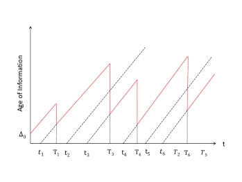
Figure 1: The $n$-server monitoring network with $S_{1},S_{2},...,S_{n}$ being the servers and $I_{1},I_{2},...,I_{m}$ being the independent information sources, sending the updates from the sources to the monitor.

Figure 2: AoI for a network with $n$ servers.

The average AoI is the limit of the average age over time $\Delta\triangleq\lim_{T\to\infty}\int_{0}^{T}\Delta(t)\big{/}T$, and for a stationary ergodic system, it is also the limit of the average age over the ensemble $\Delta=\lim_{t\to\infty}\mathbb{E}[\Delta(t)]$.

In the paper, we view our system as a stochastic hybrid system (SHS) and apply a method first introduced in [yates2018age] in order to calculate AoI. We can thus obtain the average AoI under LCFS with preemption in service, or in short, LCFS.

In SHS, the state is composed of a discrete state and a continuous state. The discrete state $q(t)\in\mathcal{Q}$, for a discrete set $\mathcal{Q}$, is a continuous-time discrete Markov chain (e.g., to represent the number of idle servers in the network), and the continuous-time continuous state $\mathbf{x}(t)=[x_{0}(t),x_{1}(t),\dots,x_{n}(t)]\in\mathbb{R}^{n+1}$ is the stochastic process for AoI. We use $x_{0}(t)$ to represent the age at the monitor, and $x_{j}(t)$ for the age at the $j$-th server, $j=1,2,\dots,n$. Graphically, we represent each state $q\in\mathcal{Q}$ by a node. For the discrete Markov chain $q(t)$, transitions happen from one state to another through directed transition edge $l$, and the time spent before the transition occurs is exponentially distributed with rate $\lambda{(l)}$. Note that it is possible to transit from the same state to itself. The transition occurs when an update arrives at a server, or an update is received at the monitor. Thus the transition rate is the update arrival rate or the service rate $\lambda{(l)}\in[\lambda_{1}^{(1)},...,\lambda_{n}^{(m)},\mu_{1},...,\mu_{n}]$. Denoted by $L^{\prime}_{{q}}$ and $L_{{q}}$ the sets of incoming and outgoing transitions of state $q$, respectively. When transition $l$ occurs, we write that the discrete state transits from $q_{l}$ to $q_{l}^{\prime}$. For instance, if we have $2$ states and considering the transition $l$ from state $1$ to state $2$, we have $q_{l}=1$ and $q_{l}^{\prime}=2$ which shows that state $2$ is an outgoing transition for state $1$ and state $1$ is an incoming transition for state $2$. For a transition, we denote that the continuous state changes from $\mathbf{x}$ to $\mathbf{x}^{\prime}$. In our problem, this transition is linear in the vector space of $\mathbb{R}^{n+1}$, i.e., $\mathbf{x}^{\prime}=\mathbf{x}A_{l}$, for some real matrix $A_{l}$ of size $(n+1)\times(n+1)$. Note that when we have no transition, the age grows at a unit rate for the monitor and relevant servers, and is kept unchanged for irrelevant servers. Hence, within the discrete state $q$, $\mathbf{x}(t)$ evolves as a piece-wise linear function in time, namely, $\frac{\partial{\mathbf{x}(t)}}{\partial{t}}=\mathbf{b}_{q}$, for some $\mathbf{b}_{q}\in\{0,1\}^{n+1}$. In other words, the age grows at a unit rate for the monitor and relevant servers; and the age is kept unchanged for irrelevant servers. For our purpose, we consider the discrete state probability

$$\pi_{\hat{q}}(t)\triangleq\mathop{\mathbb{E}}[\delta_{\hat{q},q(t)}]=P[q(t)=\hat{q}],$$ (1)

and the correlation between the continuous state $\mathbf{x}(t)$ and the discrete state $q(t)$:

$$\mathbf{v}_{\hat{q}}=[v_{\hat{q}0}(t),\dots,v_{\hat{q}n}(t)]\triangleq\mathop{\mathbb{E}}[\mathbf{x}(t)\delta_{\hat{q},q(t)}].$$ (2)

Here $\delta_{\cdot,\cdot}$ denotes the Kronecker delta function. When the discrete state $q(t)$ is ergodic, $\mathbf{\pi}_{q}(t)$ converges uniquely to the stationary probability ${\mathbf{\pi}}_{q}$, for all $q\in\mathcal{Q}$. We can find these stationary probabilities from the following set of equations knowing that $\sum_{q\in\mathcal{Q}}\pi_{q}=1$,

$${\mathbf{\pi}}_{{q}}\sum_{l\in L_{{q}}}\lambda{(l)}=\sum_{l\in L^{\prime}_{{q}}}\lambda{(l)}{\mathbf{\pi}}_{q_{l}}.\quad{q}\in\mathcal{Q}$$

A key lemma we use to develop AoI for our LCFS queue model is the following from [yates2018age], which was derived from the general SHS results in [hespanha2006modelling].

Lemma 1.

[yates2018age] If the discrete-state Markov chain $q(t)$ is ergodic with stationary distribution ${\pi}$ and we can find a non-negative solution of $\{{\mathbf{v}}_{{q}},{q}\in\mathcal{Q}\}$ such that

$${\mathbf{v}}_{{q}}\sum_{l\in L_{{q}}}\lambda{(l)}=\mathbf{b}_{{q}}{\pi}_{{q}}+\sum_{l\in L^{\prime}_{{q}}}\lambda{(l)}{\mathbf{v}}_{q_{l}}A_{l},\quad{q}\in\mathcal{Q},$$ (3)

then the average age of information is given by

$$\Delta=\sum_{{q}\in\mathcal{Q}}{v}_{{q}{0}}.$$ (4)

III AoI in Homogeneous Networks

III-A Single Source Multiple Sensors

In this section, we present AoI calculation with the LCFS queue for the single-source $n$-server homogeneous network. In this network, upon arrival of a new update, each server immediately drops any previous update in service and starts to serve the new update. Note that to compute the average AoI, Lemma 1 requires solving $|\mathcal{Q}|(n+1)$ linear equations of $\{{\mathbf{v}}_{{q}},{q}\in\mathcal{Q}\}$. To obtain explicit solutions for these equations, the complexity grows with the number of discrete states. Since the discrete state typically represents the number of idle servers in the system for homogeneous servers, $|\mathcal{Q}|$ should be $n+1$. In the following, we introduce a method inspired by [yates2018status] to reduce the number of discrete states and efficiently describe the transitions.

We define our continuous state $\mathbf{x}$ at a time as follows: the first element of $\mathbf{x}$ is AoI at the monitor ($x_{0}$), the second is always the freshest update among all updates in the servers, the third is always the second freshest update in the servers, etc. With this definition we always have $x_{1}\leq x_{2}\leq....\leq x_{n}$, for any time. Note that the index $i$ of $x_{i}$ does not represent a physical server index, but the $i$-th smallest age of information among the $n$ servers. The physical server index for $x_{i}$ changes with each transition. We say that the server corresponding to $x_{i}$ is the $i$-th virtual server.

A transition $l$ is triggered by (i) the arrival of an update at a server, or (ii) the delivery of an update to the monitor. Recall that we use $\mathbf{x}$ and $\mathbf{x}^{\prime}$ to denote AoI continuous state vector right before and after the transition $l$.

When one update arrives at the monitor and the server for that update becomes idle, we put a fake update to the server using the method introduced in [yates2018status]. Thus we can reduce the calculation complexities and only have one discrete state indicating that all servers are virtually busy. We denote this state by $q=0$. In particular, we put the current update that is in the monitor to an idle server until the next update reaches this server. This assumption does not affect our final calculation for AoI, because even if the fake update is delivered to the monitor, AoI at the monitor does not change.

When an update is delivered to the monitor from the $k$-th virtual server, the server becomes idle and as previously stated, receives the fake update. The age at the monitor becomes $x^{\prime}_{0}=x_{k}$, and the age at the $k$-th server becomes $x^{\prime}_{k}=x^{\prime}_{0}=x_{k}$. In this scenario, consider the update at the $j$-th virtual server, for $j>k$. Its delivery to the monitor does not affect AoI since it is older than the current update of the monitor, i.e., $x_{j}\geq x_{k}=x^{\prime}_{0}$. Hence, we can adopt a fake preemption where the update for the $j$-th virtual server, for all $k\leq j\leq n$, is preempted and replaced with the fake current update at the monitor. Physically, these updates are not preempted and as a benefit, the servers do not need to cooperate and can work in a distributed manner.

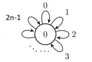
Figure 3: SHS for our model with $n$ servers.

$l$	$\lambda{(l)}$	$\mathbf{x}^{\prime}$ =$\mathbf{x}A_{l}$
$0$	$\lambda$	$[x_{0},0,x_{2},x_{3},x_{4},...,x_{n}]$
$1$	$\lambda$	$[x_{0},0,x_{1},x_{3},x_{4},...,x_{n}]$
$2$	$\lambda$	$[x_{0},0,x_{1},x_{2},x_{4},...,x_{n}]$
	$\vdots$	$\vdots$
$n-1$	$\lambda$	$[x_{0},0,x_{1},x_{2},x_{3},..,x_{n-1}]$
$n$	$\mu$	$[x_{1},x_{1},x_{1},x_{1},...,x_{1}]$
$n+1$	$\mu$	$[x_{2},x_{1},x_{2},x_{2},...,x_{2}]$
$n+2$	$\mu$	$[x_{3},x_{1},x_{2},x_{3},...,x_{3}]$
	$\vdots$	$\vdots$
$2n-1$	$\mu$	$[x_{n},x_{1},x_{2},x_{3},...,x_{n}]$

Table I: Table of transformation for the Markov chain in Figure 3.

By utilizing virtual servers, fake update, and fake preemption, we reduce SHS to a single discrete state with linear transition $A_{l}$. We illustrate our SHS with discrete state space of $Q=\{0\}$ in Figure 3. The stationary distribution ${\pi}_{0}$ is trivial and ${\pi}_{0}=1$. We set $\mathbf{b}_{q}=[1,...,1]$ which indicates that the age at the monitor and the age of each update in the system grows at a unit rate. The transitions are labeled $l\in\{0,1,...,2n-1\}$ and for each transition $l$ we list the transition rate and the transition mapping in Table I. For simplicity, we drop the index $q=0$ in the vector $\mathbf{v}_{0}$, and write it as $\mathbf{v}=[v_{0},v_{1},\dots,v_{n}]$. Because we have one state, $\mathbf{x}A_{l}$ and $\mathbf{v}A_{l}$ are in correspondence. Next, we describe the transitions in Table I.

Case I. $l=0,1,..,n-1:$ When a fresh update arrives at virtual server $l+1$, the age at the monitor remains the same and $x_{l+1}$ becomes zero. This server has the smallest age, so we take this zero and reassign it to the first virtual server, namely, $x^{\prime}_{1}=0$. In fact virtual servers $1,2,\dots,l+1$ all get reassigned virtual server numbers. Specifically, after transition $l$, virtual server $l+1$ becomes virtual server $1$, and virtual server $1$ becomes virtual server $2$,…, virtual server $l$ becomes virtual server $l+1$. The transition rate is the arrival rate of the update, $\lambda$. The matrix $A_{l}$ is

$$\bordermatrix{\leavevmode\nobreak\ &0&1&2&\dots&l+1&l+2&\dots&n\cr 0&1&&&&&&&\cr 1&&0&1&&&&&\cr\vdots&&&&\ddots&&&&\cr l&&&&&1&&&\cr l+1&&&&&&0&&\cr l+2&&&&&&1&&\cr\vdots&&&&&&&\ddots&\cr n&&&&&&&&1\cr}.$$ (5)

Case II. $l=n,n+1,..,2n-1:$ When an update is received at the monitor from virtual server $l+1-n$, the age at the monitor changes to $x_{l+1-n}$ and this server becomes idle. Using fake updates and fake preemption we assign $x^{\prime}_{j}=x_{l+1-n}$, for all $l+1-n\leq j\leq n$. The transition rate is the service rate of a server, $\mu$. The matrix $A_{l}$ is

(6)