Subharmonic oscillations in stochastic systems under periodic driving

Abstract

Subharmonic response is a well known phenomena in, e.g., deterministic nonlinear dynamical systems. We investigate the conditions under which such subharmonic oscillations can persist for a long time in open systems with stochastic dynamics due to thermal fluctuations. In contrast to stochastic autonomous systems in a stationary state, for which the number of coherent oscillations is fundamentally bounded by the number of states in the underlying network, we demonstrate that in periodically driven systems, subharmonic oscillations can, in principle, remain coherent forever, even in networks with a small number of states. We also show that, inter alia, the thermodynamic cost rises only logarithmically with the number of coherent oscillations in a model calculation and that the possible periods of the persistent subharmonic response grow linearly with the number of states. We argue that our results can be relevant for biochemical oscillations and for stochastic models of time-crystals.

I Introduction

An important class of nonequilibrium systems are those driven time-periodically, which includes systems in contact with a heat bath described by stochastic dynamics Brandner et al. (2015); Raz et al. (2016); Barato and Seifert (2016) and closed quantum system with a time-periodic Hamiltonian Moessner and Sondhi (2017). Periodically driven systems display quite rich phenomena that have been unveiled recently. Examples range from the realization of micro-sized heat engines Schmiedl and Seifert (2008); Blickle and Bechinger (2012); Martínez et al. (2016) for systems in contact with a heat bath to many body localization Ponte et al. (2015); Lazarides et al. (2015); Abanin et al. (2016) for closed quantum systems.

A rather basic issue that has not been investigated in detail yet concerns the onset of sub-harmonic oscillations, i.e., oscillations of some observable with a period larger than the period of the driving in a periodically driven system in contact with a heat bath. Does noise necessarily eliminate these oscillations in a finite system? For how long can they survive? What is the relation between the coherence of these noisy oscillations and energy dissipation? These are particularly relevant questions within the following two contexts.

First, temporal oscillations are an essential physical phenomena in living systems. Examples include the cell cycle Ferrell et al. (2011), bacterial circadian rhythms Nakajima et al. (2005); Dong and Golden (2008); Johnson et al. (2011) and other biochemical oscillations Goldbeter (1997); Novák and Tyson (2008). Genetic oscillators have also been designed in synthetic biology Elowitz and S. (2000); Kim and Winfree (2011); Potvin-Trottier et al. (2016). Noise can play an important role in these phenomena, due to the low number of constituents in a biological system such as a cell. In fact, the effect of noise in such oscillations has been extensively investigated Barkai and Leibler (2000); Gonze et al. (2002); Meinhold and Schimansky-Geier (2002); Falcke (2003); McKane et al. (2007).

Most of the analysis of this fundamental issue has been restricted to autonomous systems that are not under the influence of periodic driving. In this case, the precision of the oscillations can be quantified by the number of coherent oscillations Morelli and Jülicher (2007); Jörg et al. (2018); Qian and Qian (2000); Cao et al. (2015); Barato and Seifert (2017), which is given by the relaxation time divided by the period of oscillation. The relation between the precision of noisy oscillations in autonomous systems and thermodynamics has received much attention recently Qian and Qian (2000); Cao et al. (2015); Barato and Seifert (2017); Nguyen et al. (2018); Fei et al. (2018); Wierenga et al. (2018); Marsland III et al. (2019).

However, biophysical oscillations often take place under the influence of a periodic signal. In fact, a striking feature about biological oscillations is the range of periods involved Goldbeter (2008). For instance, if we consider oscillations within a cell, calcium oscillations Falcke (2004) can have a period of the order of minutes, whereas circadian clocks have a period of a day. Therefore, generalizing this example, a relevant question is whether a fast periodic signal influences the precision of oscillations that happen at a slower time-scale. In other words, can a fast signal with, say, a period of the order of seconds or minutes lead to precise oscillations with a period of a day?

Second, a main feature of so called time-crystals sach15 ; Khemani et al. (2016); Else et al. (2016) is a subharmonic response of an observable. These are many-body closed quantum systems that also display spatial long-range order as a main feature. Experimental realizations of time-crystals have been performed in Zhang et al. (2017); Choi et al. (2017). Time-crystals can also be observed in dissipative open systems in contact with a heat bath Lazarides and Moessner (2017); Yao et al. (2018); gong18 ; wang18 ; gamb19 . Hence, the fundamental limits of the effect of thermal noise on subharmonic oscillations can become relevant for such time-crystals as well.

The general purpose of this paper is to provide a first answer to the questions raised above about subharmonic oscillations in a stochastic systems under the influence of periodic driving. Our main result is that even in a finite system with thermal fluctuations, sub-harmonic oscillations can survive for an arbitrarily long time, with no fundamental limit. We prove this result by introducing a simple model that exhibits an indefinite number of coherent subharmonic oscillations in a particular limit. Such a divergent number of coherent oscillations in periodically driven systems is in contrast with the oscillatory behavior in autonomous systems, for which the number of coherent oscillation is fundamentally limited by the number of states of the underlying network Barato and Seifert (2017).

We also show that the trade-off between energy dissipation and the number of coherent oscillations is always more advantageous for our periodically driven model as compared to an autonomous system, if the number of coherent oscillations is large. Finally, we discuss a mathematical condition on the so-called fundamental matrix from Floquet theory that leads to restrictions on the possible number of coherent subharmonic oscillations that can be achieved in a periodically driven system.

II General setup

We consider a Markov process with $\Omega$ discrete states and continuous time $t$. The transition rate from state $i$ to state $j$ at time $t$ is denoted by $w_{ij}(t)$. These transition rates are time-periodic with a period $\tau_{\textrm{sig}}$, i.e., $w_{ij}(t+\tau_{\textrm{sig}})=w_{ij}(t)$. The time evolution of the probability to be in state $i$ at time $t$, which is denoted $p_{i}(t)$, follows the master equation

$$\frac{d}{dt}\mathbf{p}(t)=\mathcal{L}(t)\mathbf{p}(t),$$ (1)

where $\mathbf{p}(t)$ is a vector with components $p_{i}(t)$ and $[\mathcal{L}(t)]_{ji}\equiv(1-\delta_{ij})w_{ij}(t)-\delta_{ij}\sum_{k}w_{ik}(t)$ are the elements of the stochastic generator $\mathcal{L}(t)$.

The solution of this equation is given by

$$\mathbf{p}(t)=\sum_{a=1}^{\Omega}C_{a}\textrm{e}^{\mu_{a}t}\mathbf{p}^{a}(t),$$ (2)

where $C_{a}$ are constants that depend on the initial condition, $\mathbf{p}^{a}(t)=\mathbf{p}^{a}(t+\tau_{\textrm{sig}})$, and $\mu_{a}$ are the so-called Floquet exponents Klausmeier (2008). The Floquet exponent with largest real part is $\mu_{1}=0$. In the long time limit, the probability converges to the eigenvector $\mathbf{p}^{1}(t)$.

Sub-harmonic oscillations with a period $\tau_{\textrm{osc}}$ are quantified by the Floquet exponent with the second largest real part $\mu_{2}=-X_{R}\pm X_{I}i$, where $\tau_{\textrm{osc}}=2\pi/X_{I}$ and $X_{R}$ is the inverse of the relaxation time. We are interested in the ratio

$$\mathcal{R}\equiv X_{I}/X_{R}.$$ (3)

The number of coherent oscillations is given by $\mathcal{R}/2\pi$. This ratio then quantifies the precision of subharmonic oscillations.

Floquet exponents can be calculated from the fundamental matrix Grimshaw (1990); Klausmeier (2008)

$$\mathcal{M}\equiv\overleftarrow{\exp}\left(\int_{0}^{\tau_{\textrm{sig}}}\mathcal{L}(t)dt\right),$$ (4)

where the arrow indicates a time-ordered exponential. The eigenvalues of this matrix $\rho_{a}$, also known as Floquet multipliers, are related to the Floquet exponents as

$$\mu_{a}=\tau_{\textrm{sig}}^{-1}\ln\rho_{a}.$$ (5)

The largest eigenvalue is $\rho_{1}=1$. The eigenvalue with the second largest real part is written as $\rho_{2}=r\textrm{e}^{i\theta}$, where $r\leq 1$. From Eq. (5), we then obtain $X_{R}=-\ln r/\tau_{\textrm{sig}}$ and $X_{I}=\theta/\tau_{\textrm{sig}}$. This last equality leads to $\tau_{\textrm{osc}}=2\pi/X_{I}=2\pi\tau_{\textrm{sig}}/\theta\geq\tau_{\textrm{sig}}$, which shows that the period of oscillation is always larger than the period of driving.

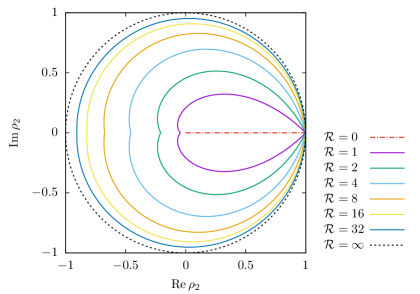
Figure 1: Contour lines for constant $\mathcal{R}$ in the complex plane of the eigenvalue $\rho_{2}$.

The contour lines for constant $\mathcal{R}$, which is defined in Eq. (3), in the complex plane of the eigenvalue $\rho_{2}$ are shown in Fig. 1. On the circle corresponding to $r=1$, the relaxation time $X_{R}^{-1}$ diverges ($\mathcal{R}\to\infty$) and subharmonic oscillations do not decay. We now provide a model with a finite number of states for which the eigenvalue $\rho_{2}$ lies on this circle in a certain limit.

III Limit of indefinite coherent subharmonic oscillations

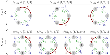
Figure 2: Illustration of the protocol for $\Omega=3$ and $\Omega=4$. The transition rates are $k_{1}\equiv k/c$ and $k_{2}\equiv k/c^{(\Omega-1)/\Omega}$.

Our model corresponds to a particle on a ring with $\Omega$ discrete states, as illustrated in Fig. 2. It can be interpreted as a colloidal particle on a ring subject to thermal noise and driven by a periodic protocol. The transition rate from state $i$ to state $i+1$ is denoted $w_{i}^{+}(t)$ and the reversed transition from state $i+1$ to state $i$ is denoted $w_{i}^{-}(t)$. For $i=\Omega$, one of the next neighbors is $i+1=1$. The period of the external signal is divided into $\Omega$ time intervals. In a generic time-interval $t\in[(n-1)\tau_{\textrm{sig}}/\Omega,n\tau_{\textrm{sig}}/\Omega]$, where $n=1,2,\ldots,\Omega$, there are three different transition rates: the reversed transition rates are given by $w_{i}^{-}=k/c^{(\Omega-1)/\Omega}$ for all states, $w_{i}^{+}=k$ for state $i=(\Omega+1-n)\mod\Omega+1$, and $w_{i}^{+}=k/c$ for all other states with $i\neq(\Omega+1-n)\mod\Omega+1$.

These transition rates fulfill detailed balance for fixed time $t$, i.e.,

$$\prod_{i=1}^{\Omega}[w_{i}^{+}(t)/w_{i}^{-}(t)]=1.$$ (6)

In terms of energies and energy barriers the transition rates can be written as $w_{i}^{+}(t)=k\textrm{e}^{E_{i}(t)-B_{i}(t)}$ and $w_{i}^{-}(t)=k\textrm{e}^{E_{i+1}(t)-B_{i}(t)}$, where $E_{i}(t)$ is the energy of state $i$, $B_{i}(t)$ is the energy barrier between states $i$ and $i+1$, and we set temperature $T=1$ and Boltzmann’s constant $k_{B}=1$ throughout. For the protocol explained in the previous paragraph, for $t\in[(n-1)\tau/\Omega,n\tau/\Omega]$, the energy difference between two neighbors is $E_{i}-E_{i+1}=[(\Omega-1)/\Omega]\ln c$ for $i=(\Omega+1-n)\mod\Omega+1$ and, $E_{i}-E_{i+1}=-(1/\Omega)\ln c$ for $i\neq(\Omega+1-n)\mod\Omega+1$.

As a main result, we obtain that this finite stochastic system exhibits indefinite subharmonic oscillations in the following particular limit. First, with $k\gg\tau_{\textrm{sig}}^{-1}$, the one internal transition with rate $k$ is much faster than the external signal. Second, $c$ is large, which leads to diverging energy differences between neighboring states, in such a way that the other transition rates are slow in comparison to the external signal, i.e., $k/c\ll\tau_{\textrm{sig}}^{-1}$ and $k/c^{(\Omega-1)/\Omega}\ll\tau_{\textrm{sig}}^{-1}$. In this limit, by numerical evaluation of the Floquet multipliers we observe that $\rho_{2}=\textrm{e}^{2\pi i/(\Omega-1)}$, which implies indefinite subharmonic oscillation with a period $\tau_{\textrm{osc}}=(\Omega-1)\tau_{\textrm{sig}}$. As discussed in Appendix A, it is also possible to obtain indefinite subharmonic oscillations with a period $\tau_{\textrm{osc}}=m\tau_{\textrm{sig}}$, where $m=2,3,\ldots,\Omega-1$, by making simple changes to this protocol. Hence, the number of possible periods grows linearly with the number of states $\Omega$.

The onset of such indefinite subharmonic oscillations in this particular limit can be understood if we consider the case $\Omega=3$ in Fig. 2 (a similar explanation holds for general $\Omega$). Let us assume that before the first period the particle starts at state $1$. During the first part of the period the particle will jump to state $2$. During the second part of the period the particle will remain trapped in state $2$ since the transition rates to leave this state are slow in comparison to the external signal. During the third part of the period the particle jumps from state $2$ to state $3$. Hence, at the end of the first period the particle will be in state $3$. For the next period the particle starts at state $3$ and jumps during the middle interval to state $1$, where it stays trapped until the end of the period. Therefore, subharmonic oscillations with a period $\tau_{\textrm{osc}}=2\tau_{\textrm{sig}}$ take place, with the particle at state $3$ at the end of odd periods and at state $1$ at the end of even periods.

In this peculiar limit, there is a perfect coupling between the dynamics of the system and the external signal that is deterministic, i.e., the system gets stuck in a state during each part of the period and transitions between states can only happen with a change of the protocol in the next part of the period. Clearly, this deterministic coupling is a general sufficient condition for the onset of subharmonic oscillations. For more complex models, we can imagine an effectively similar piecewise protocol that traps the system in some region of phase space in each part of the protocol. For such complex models, an observable that takes different values for these different regions of phase space will then display indefinite subharmonic oscillations. Hence, our model serves as a general guiding principle to obtain indefinite coherent subharmonic oscillations.

IV Relation between number of coherent oscillations and energy dissipation

Figure 3: Stroboscopic plot of the correlation function $C_{1,1}(t)$, which is the the probability to be in state $1$ at time $t$ given that the system started at state $1$. Parameters are set to $\Omega=145$, $k=600$, $\tau_{\textrm{sig}}=1$, and $c=10^{6}$. The result from the numerics is $\tau_{\textrm{osc}}\simeq 146\tau_{\textrm{sig}}$ and $R\simeq 2347$. In the discussion given in the main text $\tau_{\textrm{sig}}=1$ is set to $10$ minutes, which implies $k=1s^{-1}$, and thus leads to a period of subharmonic oscillations close to one day.

We now compare this periodically driven system to an autonomous system, modeled as a Markov process with time-independent transition rates, showing coherent oscillations. Two factors that limit the number of coherent oscillations in such autonomous system are the number of states and energy dissipation Barato and Seifert (2017). In an autonomous system with $\Omega$ states, $\mathcal{R}\leq\cot(\pi/\Omega)$, where $\mathcal{R}$ for an autonomous system is defined as the ratio of imaginary and real parts of the second largest eigenvalue associated with the Markov generator. In Fig. 3, we illustrate the fact that a fast periodic signal can increase the precision of oscillations on a slower time-scale beyond the limits that would be achievable in the absence of the signal. The period of the signal is set to $\tau_{\textrm{sig}}=10$ minutes, from numerical evaluation we obtain that the period of subharmonic oscillations is $\tau_{\textrm{osc}}\simeq 1$ day and $\mathcal{R}\simeq 2347$. This number is much larger than the fundamental limit for an autonomous system with $\Omega=145$ states, which is $\mathcal{R}=\cot(\pi/145)\simeq 46$.

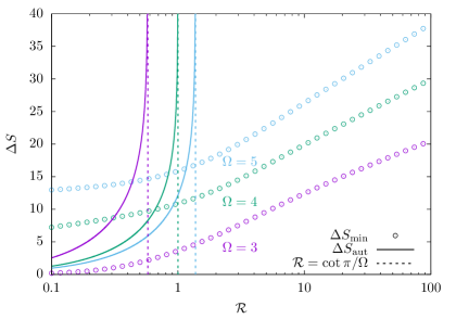
Figure 4: Entropy change per period of oscillation as a function of $\mathcal{R}$ for an autonomous system $\Delta S_{\textrm{aut}}$ and a periodically driven system $\Delta S_{\textrm{min}}$, where $\Delta S_{\textrm{min}}$ is obtained with a numerical minimization over the parameters $c$ and $k$. The vertical dashed lines represent the bound for autonomous systems $\cot(\pi/\Omega)$.

Let us now analyze the thermodynamic cost. In the limit where the model achieves indefinite subharmonic oscillations, energy differences have to be large, i.e., $\ln c\gg 1$. This condition implies that the entropy production that characterizes the thermodynamic cost diverges. The expression for the rate of entropy production Seifert (2012)

$$\sigma=\tau_{\textrm{sig}}^{-1}\int_{0}^{\tau_{\textrm{sig}}}dt\sum_{i,j}p_{i}^{1}(t)w_{ij}(t)\ln(w_{ij}(t)/w_{ji}(t)),$$ (7)

where $p^{1}_{i}(t)=p^{1}_{i}(t+\tau_{\textrm{sig}})$ is the time-periodic distribution, leads to the amount of entropy change in one period of subharmonic oscillation as $\Delta S\equiv\sigma\tau_{\textrm{osc}}$.

For the comparison of the trade-off between thermodynamic cost and $\mathcal{R}$ between our model and an autonomous system, we consider the following model for an autonomous system. A particle jumps on a ring with $\Omega$ states. The time-independent transition rates are given by $w_{i}^{+}=k\textrm{e}^{F/\Omega}$ and $w_{i}^{-}=k$, where $F=\ln\prod_{i=1}^{\Omega}[w_{i}^{+}/w_{i}^{-}]$ is the force that drives the autonomous system out of equilibrium. This particular choice of uniform rates $w_{i}^{+}$ and $w_{i}^{-}$ maximizes $\mathcal{R}$ for a fixed force $F$ Barato and Seifert (2017). For this model $\mathcal{R}=\cot(\pi/\Omega)\tanh(F/(2\Omega))$ and the thermodynamic cost of one period of oscillation is $\Delta S_{\textrm{aut}}\equiv\sigma\tau_{\textrm{osc}}=2\pi F/[\Omega\sin(2\pi/\Omega)]$ Barato and Seifert (2017).

In Fig. 4, we compare the thermodynamic cost per period that is required to obtain a certain number of coherent oscillations for both the periodically driven system and the autonomous system. For the periodically driven system, we have performed a numerical minimization of $\Delta S$ with the constraint that $\mathcal{R}$ is fixed. The free parameters in this minimization are $k$ and $c$. As expected, the amount of required thermodynamic cost increases with $\mathcal{R}$. In particular, for the periodically driven system the thermodynamic cost increases logarithmic with $\mathcal{R}$. For large enough $\mathcal{R}$ the required cost for the periodically driven system is smaller than the one for the autonomous system. This property is a consequence of the fact that the autonomous system is bounded by $\mathcal{R}\leq\cot(\pi/\Omega)$ and this bound is reached at a limit of diverging thermodynamic cost, whereas the periodically driven system is not constrained by this bound.

V Generic constraints

We finally discuss generic, model independent constraints on sub-harmonic oscillations. The mathematical properties of the fundamental matrix $\mathcal{M}$ in Eq. (4) restrict the accessible region in the complex plane of the eigenvalue $\rho_{2}$. First this matrix is a stochastic matrix, i.e., all elements are positive and the sum of the elements in a column is $1$. Dmitriev and Dynkin dmit45 ; dmit46 ; swif72 have shown that the eigenvalue $\rho_{2}$ of such a stochastic matrix is constrained to lie in the regions plotted in Fig. 5 for $\Omega=3$ and $\Omega=4$.

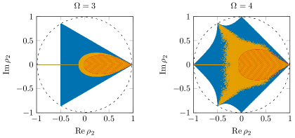
Figure 5: Domain of the the possible eigenvalues $\rho_{2}$ for $\Omega=3$ and $\Omega=4$. The larger blue region represents the constraint on stochastic matrices obtained in dmit45 ; dmit46 . The yellow scatter plots were generated with random matrices that fulfill the constraint in Eq. (8). The region inside the smaller red line represents $\mathcal{R}\leq\cot(\pi/\Omega)$.

Second, the fundamental matrix $\mathcal{M}$ is an embeddable matrix good70 ; Davies (2010), which means that it must fulfill the constraint

$$0\leq\textrm{det}\mathcal{M}\leq\prod_{i=1}^{\Omega}M_{ii}.$$ (8)

To study the effects of Eq. (8) on the eigenvalue $\rho_{2}$ we have generated random matrices that fulfill this constraint and calculated their eigenvalues numerically for $\Omega=3$ and $\Omega=4$. The results indicate that this condition lead to a region smaller than the region for general stochastic matrices, as shown in Fig. 5. In particular, the accessible region on the circle with $r=1$, where $\rho_{2}=r\textrm{e}^{i\theta}$, are the points $\rho=\textrm{e}^{2\pi i/m}$, where $m=2,3,\ldots,\Omega-1$. We have confirmed this result up to $\Omega=6$. This numerics suggests that for a stochastic system with $\Omega$ states and an indefinite number of sub-harmonic oscillations, the period of oscillation is given by $\tau_{\textrm{osc}}=m\tau_{\textrm{sig}}$, where $m=2,3,\ldots,\Omega-1$. Indeed these are the periods of subharmonic oscillations that we have obtained in our model. For an autonomous system corresponding to a continuous time Markov process with constant transition rates, we have $\mathcal{R}\leq\cot(\pi/\Omega)$ Barato and Seifert (2017). This restriction leads to the smaller regions shown in Fig. 5.

VI Conclusion

In summary, we have shown that, in principle, subharmonic oscillations in a finite, periodically driven system subjected to thermal noise can survive for an arbitrarily long time. In contrast to autonomous systems, the number of states does not impose any fundamental constraint on the maximal number of coherent oscillations. We have analyzed the trade-off relation between the number of coherent oscillations and energy dissipation for our model, showing that an increase in energy dissipation can lead to a larger number of coherent oscillations and that a periodically driven system can achieve the same number of coherent oscillations with a smaller energy budget compared to an autonomous system.

Our work raises a few fundamental questions related to the relation between thermodynamics and subharmonic oscillations in periodically driven systems. Is a diverging rate of energy dissipation that we found in our model a necessary condition to achieve the formal limit of indefinite subharmonic oscillations? What are the optimal protocols that minimize energy dissipation for a given number of coherent oscillations? What is the minimal energy budget for a given number of coherent oscillations? Furthermore, analyzing the thermodynamics of stochastic models for time-crystals, such as the one introduced in Yao et al. (2018), is an interesting direction for future work. The deterministic coupling leading to indefinite oscillations introduced here can be helpful to build such models.

Concerning biochemical oscillations, we have introduced the idea that a fast periodic signal can dramatically improve the coherence of oscillations with a longer period. Understanding under which conditions this feature takes place in more realistic and complex models for biochemical oscillations under the influence of such a signal is an appealing future step. This idea could, in principle, be used to build precise synthetic biochemical oscillators in an experimental setup where the system is under the influence of a periodic signal. Furthermore, an experimental verification of a large number of coherent subharmonic oscillations in a periodically driven finite system with thermal fluctuations could be realized with laser-induced modulated energy landscapes for a driven colloidal particle, see e.g. curt02 ; blic07 ; mart16a ; loza16 ; Gavr17 , by mimicking the simple model we have used as a proof of concept.

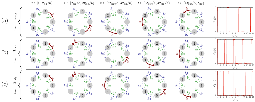
Figure 6: Three different protocols for $\Omega=5$ states. (a) Protocol in the main text with $\tau_{\mathrm{osc}}=4\tau_{\mathrm{sig}}$. (b) Protocol with $\nu=1$ anticlockwise steps, which leads to $\tau_{\mathrm{osc}}=3\tau_{\mathrm{sig}}$. (c) Protocol with $\nu=2$ anticlockwise steps, which leads to $\tau_{\mathrm{osc}}=2\tau_{\mathrm{sig}}$. On the right, the respective correlation function $C_{1,1}(t)$, which is the probability to be in state $1$ given that initially the particle was in state $1$, obtained from numerical simulations for $k=100$, $k_{1}=10^{-4}$, $k_{2}\approx 1.6\cdot 10^{-3}$ and $\tau_{\mathrm{sig}}=1$.

Appendix A Protocols for indefinite subharmonic oscillations with different periods

For the specific protocol discussed in the main text, which is sketched in the upper panel of Fig.  6 for $\Omega=5$ states, an indefinite number of subharmonic oscillations sets in for the limit $k_{1},k_{2}\ll\tau_{\mathrm{sig}}^{-1}\ll k$. The period of oscillations is $\tau_{\mathrm{osc}}=(\Omega-1)\tau_{\mathrm{sig}}$. For $\Omega=5$ we can understand this result in the following way. Consider a particle initially in state $1$ in the upper panel of Fig. (6). For this particular limit, after the first period the particle will be in state $3$. In the susequent periods the particle will move one position in the anti-clockwise direction per period, going to state $4$ after the second period and to state $5$ after the third period. After the fourth period the particle will be back at state $1$. Hence, the model displays subharmonic oscillations with $\tau_{\mathrm{osc}}=4\tau_{\mathrm{sig}}$.

Guided by this simple dynamics, we construct protocols, which have periods of subharmonic oscillations given by $\tau_{\mathrm{osc}}=m\tau_{\mathrm{sig}}$ with $m=2,3,\dots,\Omega-1$. They are obtained by the following modifications in relation to the protocol in the main text. In the standard protocol the transition associated with the strongest rate $k$ moves one clockwise position after each protocol step. In the modified protocol, the rate $k$ moves one anti-clockwise position for each of the first $\nu$ steps. Then, in the next step, this rate $k$ moves $\nu+1$ positions in the clockwise direction, going to the transition from state $\Omega$ to state $1$. In the subsequent steps, the transition rate $k$ moves one position in the clockwise direction. For $\Omega=5$, these modified protocols with $\nu=1$ and $\nu=2$ are shown in Fig. 6. From this figure one can see that the period of oscillation for a protocol with $\nu$ anti-clockwise steps is $\tau_{\mathrm{osc}}=(\Omega-1-\nu)\tau_{\mathrm{sig}}$.

References

- Brandner et al. (2015) K. Brandner, K. Saito, and U. Seifert, Phys. Rev. X 5, 031019 (2015).
- Raz et al. (2016) O. Raz, Y. Subaşı, and C. Jarzynski, Phys. Rev. X 6, 021022 (2016).
- Barato and Seifert (2016) A. C. Barato and U. Seifert, Phys. Rev. X 6, 041053 (2016).
- Moessner and Sondhi (2017) R. Moessner and S. Sondhi, Nature Phys. 13, 424 (2017).
- Schmiedl and Seifert (2008) T. Schmiedl and U. Seifert, EPL 81, 20003 (2008).
- Blickle and Bechinger (2012) V. Blickle and C. Bechinger, Nature Phys. 8, 143 (2012).
- Martínez et al. (2016) I. A. Martínez, É. Roldán, L. Dinis, D. Petrov, J. M. Parrondo, and R. A. Rica, Nature Phys. 12, 67 (2016).
- Ponte et al. (2015) P. Ponte, Z. Papić, F. M. C. Huveneers, and D. A. Abanin, Phys. Rev. Lett. 114, 140401 (2015).
- Lazarides et al. (2015) A. Lazarides, A. Das, and R. Moessner, Phys. Rev. Lett. 115, 030402 (2015).
- Abanin et al. (2016) D. A. Abanin, W. D. Roeck, and F. Huveneers, Ann. Phys. 372, 1 (2016).
- Ferrell et al. (2011) J. E. Ferrell, T. Y.-C. Tsai, and Q. Yang, Cell 144, 874 (2011).
- Nakajima et al. (2005) M. Nakajima, K. Imai, H. Ito, T. Nishiwaki, Y. Murayama, H. Iwasaki, T. Oyama, and T. Kondo, Science 308, 414 (2005).
- Dong and Golden (2008) G. Dong and S. S. Golden, Curr. Opin. Microbiol. 11, 541 (2008).
- Johnson et al. (2011) C. H. Johnson, P. L. Stewart, and M. Egli, Annu. Rev. Biophys. 40, 143 (2011) .
- Goldbeter (1997) A. Goldbeter, Biochemical Oscillations and Cellular Rhythms: The Molecular Bases of Periodic and Chaotic Behaviour (Cambridge Univ. Press, 1997).
- Novák and Tyson (2008) B. Novák and J. J. Tyson, Nature Rev. Mol. Cell Biol. 9, 981 (2008).
- Elowitz and S. (2000) M. B. Elowitz and S. Leibler, Nature 403, 335 (2000).
- Kim and Winfree (2011) J. Kim and E. Winfree, Mol. Syst. Biol. 7, 465 (2011).
- Potvin-Trottier et al. (2016) L. Potvin-Trottier, N. D. Lord, G. Vinnicombe, and J. Paulsson, Nature 538, 514 (2016).
- Barkai and Leibler (2000) N. Barkai and S. Leibler, Nature 403, 267 (2000).
- Gonze et al. (2002) D. Gonze, J. Halloy, and P. Gaspard, The J. Chem. Phys. 116, 10997 (2002) .
- Meinhold and Schimansky-Geier (2002) L. Meinhold and L. Schimansky-Geier, Phys. Rev. E 66, 050901 (2002).
- Falcke (2003) M. Falcke, Biophys J. 84, 42 (2003).
- McKane et al. (2007) A. J. McKane, J. D. Nagy, T. J. Newman, and M. O. Stefanini, J. Stat. Phys. 128, 165 (2007).
- Morelli and Jülicher (2007) L. G. Morelli and F. Jülicher, Phys. Rev. Lett. 98, 228101 (2007).
- Jörg et al. (2018) D. J. Jörg, L. G. Morelli, and F. Jülicher, Phys. Rev. E 97, 032409 (2018).
- Qian and Qian (2000) H. Qian and M. Qian, Phys. Rev. Lett. 84, 2271 (2000).
- Cao et al. (2015) Y. Cao, H. Wang, Q. Ouyang, and Y. Tu, Nature Phys. 11, 772 (2015).
- Barato and Seifert (2017) A. C. Barato and U. Seifert, Phys. Rev. E 95, 062409 (2017).
- Nguyen et al. (2018) B. Nguyen, U. Seifert, and A. C. Barato, J. Chem. Phys. 149, 045101 (2018) .
- Fei et al. (2018) C. Fei, Y. Cao, Q. Ouyang, and Y. Tu, Nature Comm. 9, 1434 (2018).
- Wierenga et al. (2018) H. Wierenga, P. R. ten Wolde, and N. B. Becker, Phys. Rev. E 97, 042404 (2018).
- Marsland III et al. (2019) R. Marsland III, W. Cui, and J. Horowitz, arXiv:1901.00548 (2019).
- Goldbeter (2008) A. Goldbeter, Curr. Biol. 18, R751 (2008).
- Falcke (2004) M. Falcke, Adv. Phys. 53, 255 (2004) .
- (36) K. Sacha, Phys. Rev. A 91, 033617 (2015).
- Khemani et al. (2016) V. Khemani, A. Lazarides, R. Moessner, and S. L. Sondhi, Phys. Rev. Lett. 116, 250401 (2016).
- Else et al. (2016) D. V. Else, B. Bauer, and C. Nayak, Phys. Rev. Lett. 117, 090402 (2016).
- Zhang et al. (2017) J. Zhang, P. Hess, A. Kyprianidis, P. Becker, A. Lee, J. Smith, G. Pagano, I.-D. Potirniche, A. C. Potter, A. Vishwanath, et al., Nature 543, 217 (2017).
- Choi et al. (2017) S. Choi, J. Choi, R. Landig, G. Kucsko, H. Zhou, J. Isoya, F. Jelezko, S. Onoda, H. Sumiya, V. Khemani, et al., Nature 543, 221 (2017).
- Lazarides and Moessner (2017) A. Lazarides and R. Moessner, Phys. Rev. B 95, 195135 (2017).
- Yao et al. (2018) N. Y. Yao, C. Nayak, L. Balents, and M. P. Zaletel, arXiv:1801.02628 (2018).
- (43) Z. Gong, R. Hamazaki, and M. Ueda, Phys. Rev. Lett. 120, 040404 (2018).
- (44) R. R. W. Wang, B. Xing, G. G. Carlo, and D. Poletti, Phys. Rev. E 97, 020202 (2018).
- (45) F. M. Gambetta, F. Carollo, M. Marcuzzi, J. P. Garrahan, and I. Lesanovsky, Phys. Rev. Lett. 122, 015701 (2019).
- Klausmeier (2008) C. A. Klausmeier, Theoret. Ecol. 1, 153 (2008).
- Grimshaw (1990) R. Grimshaw, Nonlinear Ordinary Differential Equations (Blackwell Scientific Publications, 1990).
- Seifert (2012) U. Seifert, Rep. Prog. Phys. 75, 126001 (2012).
- (49) N. Dmitriev, E. Dynkin, C. R. (Doklady) Acad. Sci. URSS 49, 159 (1945).
- (50) N. Dmitriev and E. Dynkin, Izv. Akad. Nauk SSSR Seria Mathem. 10, 167 (1946).
- (51) J. Swift, MSc Thesis, McGill University, (1972).
- (52) G. Goodman, Z. Wahrscheinlichkeit. 16, 165 (1970).
- Davies (2010) E. B. Davies, Electronic J. Prob. 15, 1474 (2010).
- (54) J. E. Curtis, B. A. Koss, and D. G. Grier, Opt. Commun. 207, 169 (2002).
- (55) V. Blickle, T. Speck, C. Lutz, U. Seifert, and C. Bechinger, Phys. Rev. Lett. 98, 210601 (2007).
- (56) I. A. Martínez, A. Petrosyan, D. Guéry-Odelin, E. Trizac, and S. Ciliberto, Nat. Phys. 12, 843 (2016).
- (57) C. Lozano, B. ten Hagen, H. Löwen, and C. Bechinger, Nat. Commun. 7, 12828 (2016).
- (58) M. Gavrilov and J. Bechhoefer, Phil. Trans. R. Soc. A 375, 20160217 (2017).