The VISCACHA survey - I. Overview and First Results

Abstract

The VISCACHA (VIsible Soar photometry of star Clusters in tApii and Coxi HuguA) Survey is an ongoing project based on deep photometric observations of Magellanic Cloud star clusters, collected using the SOuthern Astrophysical Research (SOAR) telescope together with the SOAR Adaptive Module Imager. Since 2015 more than 200 hours of telescope time were used to observe about 130 stellar clusters, most of them with low mass (M < 10⁴ M$\odot$) and/or located in the outermost regions of the Large Magellanic Cloud and the Small Magellanic Cloud. With this high quality data set, we homogeneously determine physical properties from statistical analysis of colour-magnitude diagrams, radial density profiles, luminosity functions and mass functions. Ages, metallicities, reddening, distances, present-day masses, mass function slopes and structural parameters for these clusters are derived and used as a proxy to investigate the interplay between the environment in the Magellanic Clouds and the evolution of such systems. In this first paper we present the VISCACHA Survey and its initial results, concerning the SMC clusters AM3, K37, HW20 and NGC796 and the LMC ones KMHK228, OHSC3, SL576, SL61 and SL897, chosen to compose a representative subset of our cluster sample. The project’s long term goals and legacy to the community are also addressed.

1 Introduction

The gravitational disturbances resulting from interactions between the Large Magellanic Cloud (LMC) and the Small Magellanic Cloud (SMC) and between these galaxies and the Milky Way (MW) are probably imprinted on their star formation histories, as strong tidal effects are known to trigger star formation across dwarf galaxies (Kennicutt et al., 1996). Gas dynamics simulations of galaxy collision and merging have shown that the properties of tidally induced features such as the Magellanic Stream and Bridge can be used to gather information about the collision processes and to infer the history of the colliding galaxies (Olson & Kwan, 1990). When applied to model the Magellanic System, present-day simulations have been able to reproduce several of the observed features of the interacting galaxies such as shape, mass and the induced star formation rates. However, it is still not clear whether the Magellanic Clouds are on their first passage, or if they have been orbiting the MW for a longer time (e.g. Mastropietro et al., 2005; Besla et al., 2007; Diaz & Bekki, 2012; Kallivayalil et al., 2013).

Putman et al. (1998) confirmed the existence of the Leading Arm, which is the counterpart of the trailing Magellanic Stream. The existence of both gas structures most likely has a tidal origin. Because of that, it is also expected that the Magellanic Stream, the Leading Arm and the Magellanic Bridge should have a stellar counterpart of the tidal effects within the Magellanic System (e.g. Diaz & Bekki, 2012). Besides, the close encounters among SMC, LMC and the MW should trigger star formation at specific epochs (Harris & Zaritsky, 2009), presumably imprinted in the age and metallicity distribution of field and cluster stars.

In the context of interacting galaxies, it is well known that the tidal forces have a direct impact over the dynamical evolution and dissolution of stellar clusters and that the intensity of these effects typically scale with galactocentric distances (Bastian et al., 2008). The outcome of these gravitational stresses imprinted on the stellar content of these systems can be diagnosed by means of the clusters structural parameters (Werchan & Zaritsky, 2011; Miholics et al., 2014) and mass distribution (Glatt et al., 2011). In a similar fashion, the effects of the galactic gravitational interactions in the Magellanic System should also be seen in the structural, kinematical and spatial properties of their stellar clusters, particularly on those on the peripheries of the LMC and SMC. Whether or not they are affected by significant disruption during their lifetime is an open question and subject of current debate (Casetti-Dinescu et al., 2014). Comparing these properties at different locations across the Magellanic Clouds is the key to unveiling the role of tidal forces over the cluster’s evolution and to map crucial LMC and SMC properties at projected distances usually not covered by previous surveys. Given the complexity of the cluster dynamics in the outer LMC and SMC, additional kinematic information might be required (e.g. radial velocities) to constraint their orbits and address the issue of possible cluster migration, both in a galactic context and between the Clouds, as such behaviour has already been seen in their stellar content (Olsen et al., 2011).

Fortunately, most of the star clusters fundamental parameters such as age, metallicity, distance, reddening and structural parameters can be inferred from photometry using well established methodologies such as simple stellar population models, N-body simulations, stellar evolution models and colour-magnitude diagrams (CMDs). These parameters, in turn, can be used to probe the 3D structure of the Magellanic Clouds and Bridge, to sample local stellar populations and also to map their chemical gradients and evolutionary history. When combined with proper motions from Gaia Collaboration et al. (2018) and with radial velocities and metallicities from a spectroscopic follow-up they can provide a wealth of additional information such as the radial metallicity gradients, still under discussion for these galaxies, the internal dynamical status and evolutionary timescales of the clusters and their 3D motions and orbits, which constrain the mass of the LMC and SMC.

Some efforts have been made to collect heterogeneous data from the literature and study the topics above (e.g. Pietrzynski & Udalski, 2000, Rafelski & Zaritsky, 2005, Glatt et al., 2010, Piatti, 2011, Palma et al., 2016, Perren et al., 2017, Parisi et al., 2009; Parisi et al., 2014, 2015, Dias et al., 2014, 2016, Nayak et al., 2016, Pieres et al., 2016 etc). However, the dispersion in the parameters due to different data qualities, analysis techniques and photometric bands used do not put hard constraints on the history of the SMC and LMC star cluster populations. This is usually one of the most compelling arguments to carry out a survey in the Magellanic Clouds.

After Putman et al. (1998), the investigation of some of these subjects has greatly benefited from several photometric surveys, some dedicated exclusively to the Magellanic Clouds. We describe the main surveys covering the Magellanic Clouds in Table 1. It can be seen that they complement each other in terms of sky coverage, filters, photometric depth, and spatial resolution. All of them give preference to large sky coverage over photometric depth at the expense of good photometry of low-mass stars in star clusters. The Hubble Space Telescope (HST) is suitable to explore this niche, but only for a few selected massive clusters given the time limitations implied in observing hundreds of low-mass ones.

Our VISCACHA (VIsible Soar photometry of star Clusters in tApii and Coxi HuguA) survey exploits the unique niche of deep photometry of star clusters and a good spatial resolution throughout the LMC, SMC, and Magellanic Bridge. In order to observe a large sample, including the numerous low-mass clusters we need large access to a suitable ground-based facility. These conditions are met at the 4.1-m Southern Astrophysical Research (SOAR) telescope combined with the SOAR Telescope Adaptive Module (SAM) using ground-layer adaptive optics (GLAO). The VISCACHA team can access a large fraction of nights at SOAR (Brazil: 31%, Chile: 10%) to cover hundreds of star clusters in the Magellanic System during a relatively short period, with improved photometric depth and spatial resolution. This combination allows us to generate precise CMDs especially for the oldest, compact clusters immersed in dense fields, which is not possible with large surveys. A more detailed description of the survey is given in Section 2.

Table 1: Summary of photometric surveys covering the Magellanic System. Future surveys (LSST, Euclid), the ones with marginal cover of the Magellanic System or that are photometrically shallow are not listed (DSS, 2MASS, Pan-STARRS, MagLiteS, ATLAS, MAGIC). Spectroscopic surveys are not listed either (APOGEE-2, Local Volume Mapper, Gaia, 4MOST).

survey	period	telescope/	typical	filters	mag.lim.	scale	total sky	main goals	main
(PI)	(observ.)	instrument	seeing			($\arcsec$/px)	coverage		refs.
MCPS (Zaritsky)	1996-1999 (+2001)	1m Swope @ LCO, Great circle camera (drift-scan)	1.2-1.8$\arcsec$	UBVI	$V<$21a	0.7	64$\deg^{2}$ (LMC) 18$\deg^{2}$ (SMC)	field SFH SMC/LMC, cluster census, reddening map	1, 2, 3, 4
VMC (Cioni)	2009-2018	4m VISTA @ ESO, VIRCAM (1∘x1∘)	0.8-1.2$\arcsec$	YJKs	$J<$21.9a	0.34	116$\deg^{2}$ (LMC) 45$\deg^{2}$ (SMC) 20$\deg^{2}$ (Bridge) 3$\deg^{2}$ (Stream)	spatially-resolved SFH, 3D structure, stellar variability	5, 6, 7, 8, 9
OGLE-IV (Udalski)	2010-2014	1.3m Warsaw @ LCO ($\diameter\sim$ 1.5∘)	1.0-2.0$\arcsec$	(B)VI	$I<$21.7 ($I<$20.5b)	0.26	670$\deg^{2}$ (SMC, LMC, Bridge)	Stellar variability	10, 11, 12, 13
STEP (Ripepi)	2011+	2.6m VST @ ESO OmegaCAM (1$\deg^{2}$)	1.0-1.5$\arcsec$	griH$\alpha$	$g<$23.5a	0.21	74$\deg^{2}$ (SMC main body) 30$\deg^{2}$ (Bridge) 2$\deg^{2}$ (Stream)	visible complement of VMC, SFH of SMC down to oldest populations	14
SMASH (Nidever)	2013-2016	4m Blanco @ CTIO DECam, NOAO (3$\deg^{2}$)	1.0-1.2$\arcsec$	ugriz	$g<$22.5a	0.27	480$\deg^{2}$ (Leading arm, SMC, LMC cores)	stellar counterpart of Leading Arm, spatially resolved SFH LMC/SMC	15, 16, 17, 18
DES (Friemanc)	2013-2018	4m Blanco @ CTIO DECam, NOAO (3$\deg^{2}$)	0.8-1.2$\arcsec$	grizY	$g<$23.7b	0.27	5000$\deg^{2}$ (Stream plus large area unrelated to SMC/LMC)	Magellanic Stream, tidal dwarf galaxies	19, 20, 21
Gaia (Prustid)	2013-2019	1.49m$\times$0.54m ($\times 2$) Gaia @ ESA (space)	$>0.1\arcsec^{e}$	G (blue, red photometer)	$G<$20.7f	0.06 $\times$ 0.18	all sky	proper motion of brightest stars, stellar variability, SFH	22, 23, 24, 25
Skymapper (Da Costa)	2014-2020	1.35m SSO @ ANU (2.4$\times$2.3$\deg^{2}$)	1.2-1.8$\arcsec$	uvgriz	$g<$18f (g$<22^{g}$)	$\sim$0.5	all Southern sky	outskirts of LMC/SMC, origin of Stream at the Bridge	26
VISCACHA (Dias)	2015+	4.1m SOAR @ Cerro Pachon / SAMI with GLAO ($3\arcmin\times 3\arcmin$)	0.8-1.0$\arcsec$ (AO$\sim$0.5$\arcsec$)	(B)VI	$V<24^{a}$	0.09 (binned)	only star clusters	star clusters of all ages, LMC, SMC, bridge, tidal effects on clusters, precise CMDs	27, 28, 29, 30

Based on the presentation by M.R. Cioni at ESO2020 workshop in 2015, updated with more surveys and details: https://www.eso.org/sci/meetings/2015/eso-2020/program.html (a) Completeness at 50% using artificial star tests in the crowded regions. (b) Completeness at 95-100%. (c) Director. (d) Project scientist. (e) Gaia is able to separate two point sources that are $>0.1\arcsec$ apart, but this is only a reference, it cannot be directly compared with ground-based telescope FWHM or resolving power. Another parameter is that Gaia can resolve stars up to a density of 0.25 star/$\arcsec^{2}$. (f) Hard limit, large uncertainty, low completeness. (g) DR1 only contains shallow survey. The full survey is expected to reach 4 mag deeper. (1) Zaritsky et al. (1996); (2) Zaritsky et al. (1997); (3) Zaritsky et al. (2002); (4) Zaritsky et al. (2004); (5) Cioni et al. (2011); (6) Piatti et al. (2015); (7) Subramanian et al. (2017); (8) Niederhofer et al. (2018); (9) Rubele et al. (2018); (10) Udalski et al. (2015); (11) Skowron et al. (2014); (12) Jacyszyn-Dobrzeniecka et al. (2016); (13) Sitek et al. (2017); (14) Ripepi et al. (2014) (15) Nidever et al. (2017) (16) Nidever et al. (2018) (17) Choi et al. (2018a) (18) Choi et al. (2018b) (19) Abbott et al. (2018) (20) Pieres et al. (2016) (21) Pieres et al. (2017) (22) Gaia Collaboration et al. (2016a) (23) Gaia Collaboration et al. (2016b) (24) van der Marel & Sahlmann (2016) (25) Helmi et al. (2018) (26) Wolf et al. (2018) (27) Dias et al. (2014) (28) Dias et al. (2016) (29) Maia et al. (2014) (30) Bica et al. (2015).

Among the topics that the VISCACHA data shall allow to address and play an important role, we list: (i) position dependence structural parameters of clusters, (ii) age-metallicity relations of star clusters and radial gradients, (iii) 3D structure of the Magellanic System in contrast with results from variable stars, (iv) star cluster formation history, (v) dissolution of star clusters, (vi) initial mass function for high- and low-mass clusters, (vii) extended main-sequence turnoffs in intermediate-age clusters, (viii) combination with kinematical information to calculate orbits, among others.

This paper is organized as follows. In Section 2 we present an overview of the VISCACHA survey. In Sections 3 and 4 we describe the observations and data reduction. The analysis we will perform on the whole data set is presented in Section 5, and the first results are shown in Section 6. Conclusions and perspectives are summarised in Section 7.

2 The VISCACHA survey

Photometric studies of Magellanic Clouds clusters are usually limited to those with the main sequence turn-off above the detection limits (Chiosi et al., 2006), which is directly related to the depth of the observations. Furthermore, crowding can also hamper the studies of many compact clusters and those immersed in rich backgrounds such as the LMC bar. This limits the sample to massive, young to intermediate-age clusters, while leaving the much more numerous low mass ones largely unexplored.

The VISCACHA survey is performing a comprehensive study of the outer regions of the Magellanic Clouds by collecting deep, high quality images of its stellar clusters using the 4.1 m SOAR telescope and its SAM Imager (SAMI).

When compared with other surveys on the Magellanic Clouds, the VISCACHA survey is reaching $>$2mag deeper than previous studies (largely based on the 2MASS, MCPS or the VMC surveys), attaining S/N $\approx$ 10 at V $\approx$ 24, which is slightly better than those achieved by SMASH ($z\sim 23.5$, $g\sim 22.5$). Furthermore, while SMASH aims to search and identify low surface brightness stellar populations across the Magellanic Clouds, the VISCACHA survey will provide local high quality data of specific targets enabling the most complete characterization of their populations. Due to the employment of the adaptive optics system, the spatial resolution achieved by VISCACHA (FWHM $\approx$ 0.5″, $V$ band) is higher than that of any other survey on the Magellanic Clouds, enabling the deblending of the stellar sources down to very crowded scenarios. Even though HST photometry (e.g. Glatt et al., 2008) is still deeper than ground based photometry, the spatial coverage of the VISCACHA survey greatly surpasses those with appropriate field of view and resolution, allowing for a larger cluster sample and a more complete understanding of these galaxy properties.

On a short term, the VISCACHA survey will deliver a high quality, homogeneous database of star clusters in the Magellanic Clouds, providing reliable physical parameters such as core and tidal radii, ellipticities, distances, ages, metallicities, mass distributions as derived from standard data reduction and analysis processes. The effects of the local tidal field over their evolution will be quantified through the analysis of their structural parameters, dynamical times, and positions within the Galactic system. Comparison of these results with models (e.g. van der Marel et al., 2009; Baumgardt et al., 2013) will provide important constraints to understand the evolution of the Magellanic Clouds.

Once a significant sample has been collected, a study of the star formation history and chemical enrichment of the star clusters located at the periphery of these galaxies will be carried out to probe the local galactic properties. Based on this dataset, several aspects concerning the evolution of these galaxies will be revisited, such as spatial dependence of age-metallicity relationship (Dobbie et al., 2014), the “V"-shaped metallicity and age gradients found in the SMC (Dias et al., 2014, 2016; Parisi et al., 2009; Parisi et al., 2015), the 3D cluster distribution, the inclination of the LMC disc, among others.

Finally, our catalogues will be matched against others (e.g. MCPS, VMC, OGLE) comprising a more complete panchromatic data set that will serve as reference for future studies of star clusters in the Magellanic Clouds. Even though this is not a public survey, it has a legacy value, therefore we intend to eventually compile an easily accessible on-line database, including photometric tables, parameter catalogues, and reduced images.

3 Observations

Historically, the VISCACHA team originated from the merging of two Brazilian teams, one of them observing star clusters in the periphery of the LMC looking for structural parameters, and the other one observing clusters in the periphery of the SMC looking for age-metallicity relation and radial gradients. Both teams started observing with the SOAR optical imager (SOI) since its commissioning in 2006, and joined forces to found the VISCACHA collaboration observing with the recently commissioned SAMI in 2015. We broadened the science case and the collaboration team, having members based in Brazil, Chile, Argentina, and Colombia so far.

Considering the observing runs 2015A, 2015B, 2016B and 2017B we have observed about 130 clusters. In order to demonstrate the methods concerning CMDs and cluster structure we use in the present study a subsample of 4 SMC and 5 LMC clusters illustrating different concentration, total brightness and physical parameters. Their $V$ images are shown in Fig. 1 and their observation log in Tab. 2. A list containing the full sample of all observed clusters up to the 2017B run is given in the appendix (Table LABEL:tab:clulist).

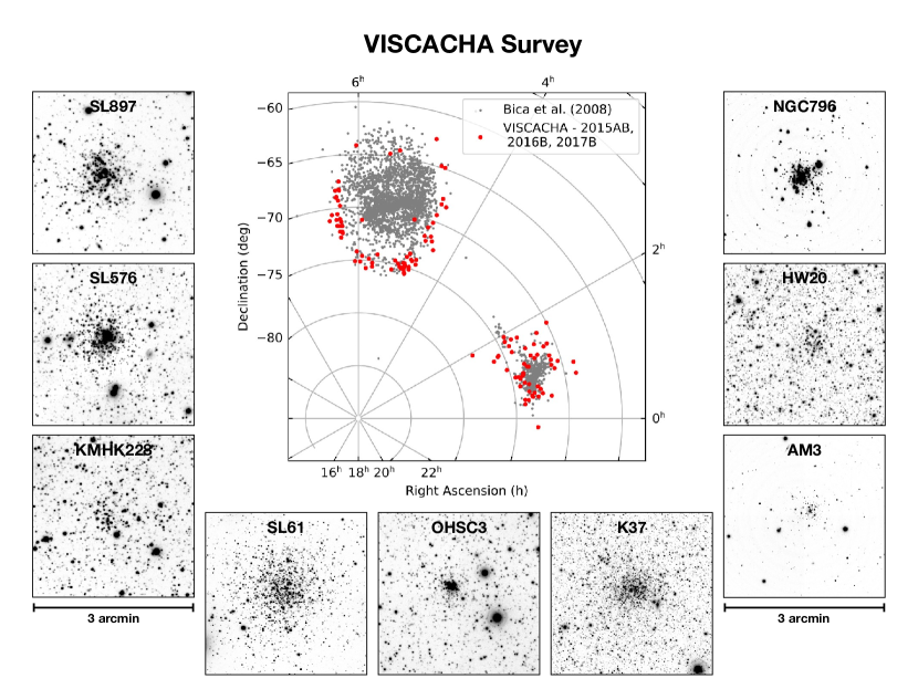
Figure 1: Central panel: present VISCACHA sample, including $\sim$130 clusters observed through 2015-2017 (red circles). Small black dots correspond to the catalogued objects in the Magellanic System by Bica et al. (2008). Surrounding panels: $V$ image of selected targets, representing the variety of cluster types in the survey.

Table 2: Log of observations only for the clusters analysed in this paper.

Name	RA	Dec	date	filter	exptime	airmass	seeing	IQ	$\tau_{0}$	AO?
	[h:m:s]	[∘:$\arcmin$:$\arcsec$]	[DD.MM.YYYY]		[sec]		[arcsec]	[arcsec]	[ms]
SMC
AM3	23:48:59	-72:56:43	04.11.2016	V, I	$6\times 200$, $6\times 300$	1.38	1.2, 1.1	0.5, 0.4	7.2, 5.7	ON
HW20	00:44:47	-74:21:46	27.09.2016	V, I	$6\times 200$, $6\times 300$	1.40	1.2, 0.9	0.6, 0.5	4.8, 6.8	ON
K37	00:57:47	-74:19:36	04.11.2016	V, I	$4\times 200$, $4\times 300$	1.44	0.8, 0.8	0.5, 0.4	7.0, 7.2	ON
NGC796	01:56:44	-74:13:10	04.11.2016	V, I	$3\times 100$, $4\times 100$	1.78	1.0, 0.9	0.6, 0.5	5.4, 6.3	ON
LMC
KMHK228	04:53:03	-74:00:14	11.01.2016	V, I	$3\times 375$, $3\times 560$	1.42	1.1, 1.0	1.1, 1.0	3.9, 3.1	ON
OHSC3	04:56:36	-75:14:29	02.12.2016	V, I	$3\times 375$, $3\times 560$	1.45	1.0, 1.0	1.0, 1.0	2.0, 2.0	OFF
SL576	05:33:13	-74:22:08	29.11.2016	V, I	$3\times 375$, $3\times 560$	1.48	1.3, 1.0	1.2, 1.0	4.3, 3.4	ON
SL61	04:50:45	-75:31:59	09.01.2016	V, I	$3\times 375$, $3\times 560$	1.64	0.9, 0.8	0.7, 0.6	7.5, 6.9	ON
SL897	06:33:01	-71:07:40	23.02.2015	V, I	$3\times 375$, $3\times 560$	1.34	1.5, 1.4	1.1, 0.9	3.5, 4.3	ON

3.1 Strategy

The overall primary goal of VISCACHA is to further investigate clusters in the outer LMC ring, and to explore the SMC halo and Magellanic Bridge clusters. A panorama of these external LMC and SMC structures and the already collected VISCACHA targets are given in Fig. 1. In the first outer LMC cluster catalogue (Lynga & Westerlund, 1963), the outer LMC ring could be inferred. It appears to be a consequence of a nearly head-on collision with the SMC, similarly to the Cartwheel scenario (Bica et al., 1998). This interaction is also responsible for the inflated SMC halo (Fig. 1). In Bica et al. (2008) these structures can be clearly seen. In that study they found 3740 star clusters in the Magellanic System. However, this number does not account for other cluster types such as embedded clusters, small associations (Hodge, 1986), and other types of objects.

The north-east outer LMC cluster distribution has also been recently discussed by Pieres et al. (2017). The outer ring is located from 5 kpc to 7 kpc from the dynamical LMC centre, but well inside its tidal radius ($\gtrsim$ 16 kpc - van der Marel & Kallivayalil, 2014). Since there is a tendency for older clusters to be located in the LMC outer disk regions (Santos et al., 2006), these objects are ideal candidates to be remnants from the LMC formation epoch. In particular, such clusters may belong to a sample without a counterpart in our Galaxy due to the different tidal field strengths, persisting as bound structures for longer times than in the Milky Way.

In the SMC, the galaxy main body can be represented by an inner ellipsoidal region, while its outer part can be sectorised as proposed by Dias et al. (2014, 2016): (i) a wing/bridge, extending eastward towards the Magellanic Bridge connecting the LMC and SMC; (ii) a counter-bridge in the northern region, which could represent the tidal counterpart of the Magellanic Bridge; (iii) a west halo on the opposite side of the bridge. These groups had also been predicted in the stellar distribution of Besla (2011) and Diaz & Bekki (2012) models and most likely have a tidal origin tied to the dynamical history of the Magellanic Clouds. The wing/bridge clusters present distinct age and metallicity gradients (Parisi et al., 2015; Dias et al., 2016) which could be explained by tidal stripping of clusters beyond 4.5 deg, radial migration, or merging of galaxies. The age and metallicity gradients in the west halo were used to propose that these clusters are moving away from the main body (Dias et al., 2016), as confirmed later by proper motion determinations from VMC survey (Niederhofer et al., 2018), HST and Gaia measurements (Zivick et al., 2018). These radial trends are crucial to charaterise the SMC tidal structures and to define a more complete picture of its history.

Photometric images with $BVI$ filters were obtained for approximately 130 clusters in the LMC, SMC and Bridge so far, during the semesters of 2015A, 2015B, 2016B and 2017B. Their distribution in the Magellanic System is shown in Fig. 1.

3.2 Instrumentation: SAMI data

Observation of our targets include short exposures to avoid saturation of the brightest stars ($V\sim 16$) and deep exposures to sample $V\sim 24$ stars with S/N $\sim$ 10. Photometric calibration of individual nights have been done by observing both Stetson (2000) (for extinction evaluation) and MCPS fields (for colour calibration) over the $B$, $V$ and $I$ filters.

SAM is a GLAO module using a Rayleigh laser guide star at $\sim$7 km from the telescope. SAM was employed with its internal CCD detector, SAMI (4K$\times$ 4K CCD), set to a gain of 2.1  e^-/ADU and a readout noise of 4.7 e^- and binned to 2$\times$2 factor, resulting in a plate scale of 0.091 arcsec/pixel with the detector covering a field-of-view of 3.1$\times$3.1 arcmin² on the sky. Peak performance of the system produce FWHM $\sim$0.4 arcsec in the $I$ band and $\sim$0.5 arcsec in the $V$ band, which still allows for adequate sampling of the point spread function (PSF), reaching a minimum size of $\sim$4.4 pixels (FWHM) in those occasions.

SAM operates at a maximum rate of 440Hz which means it can only correct the effects of ground-layer atmospheric turbulence if the coherence time is $\tau_{0}>2.3$ms. The closer the $\tau_{0}$ is to this limit the worse is the AO correction. In fact, Table 2 shows that although all clusters were observed under similar seeing and airmass, the delivered image quality (IQ) varied from target to target. The variation is explained by the free-atmosphere seeing variations (above 0.5km) that are not corrected by GLAO. The SMC clusters were observed under better conditions of the free-atmosphere and as a consequence have deeper photometry reaching the goals of the ideal performance for the VISCACHA data.

For the last observation period (2017B), we only took short exposures in the B filter since SAM has optimal performance in $V$ and $I$ bands, which decreases towards blue wavelengths. This strategy allowed us to increase our number of targets observed with AO, improving the efficiency of the survey. It is worth noticing that even for observations with relatively high airmass ($X\sim 1.3-1.7$) the instrument performed well, improving the image quality, whenever the atmospheric seeing was around 1 arcsec.

4 Data Reduction

4.1 Processing

The data were processed in a standard way with IRAF, using automated scripts designed to work on SAM images. Pre-reduction included bias subtraction and division by skyflats using the ccdred package and cosmic rays removal with the crutil package. Correction of the camera known optical distortion was also done, as it is large enough ($\sim$10%) to shift stellar positions by more than 1 arcsec in some image areas. Subsequent astrometric calibration was performed with the imcoords package, using astrometric references from 2MASS, GSC-2.3 and MCPS catalogues, and ensuring a typical accuracy better than $\sim 0.1$ arcsec for all our images. See Fraga et al. (2013) for further details in the processing and astrometric calibration procedures.

The final processing step was to register the repeated long exposures in each filter to a common WCS frame and to stack them into a deeper mosaic using the IRAF immatch package. To preserve image quality of our mosaics the co-added images were weighted according to their individual seeing ($\propto FWHM^{-2}$). This, allied with the good quality of our astrometric solutions, resulted in very little degradation of the stellar PSF ($<$ 10%) in the resulting mosaics.

4.2 Photometry

Stellar photometry was done using a modified version of the Starfinder code (Diolaiti et al., 2000), which performs isoplanatic high resolution analysis of crowded fields by extracting an empirical PSF from the image and cross-correlating it with every point source detected above a defined threshold. The modifications were aimed mainly at automatising the code, minimising the user intervention. Modelling of each image PSF was carried out by using 20 to 50 bright, unsaturated stars presenting no bright neighbour closer than 6 FWHM. This initial PSF was used to model and remove faint neighbours around the initially selected stars, which were then reprocessed to generate a definitive PSF. Fig. 2 shows the resulting PSF of the deep $I$ mosaic of the cluster Kron 37 after the subtraction of secondary sources around the model stars. Even though the FWHM is only about 5 pixels, the PSF profile is clearly defined up to a distance of 30 pixels ($\sim$6 FWHM), well into the sky region.

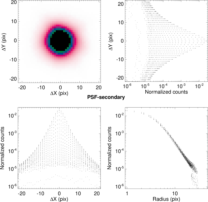
Figure 2: Empirical PSF of Kron 37 in the I-band as shown by its image (top-left), marginal profile along the X-axis (bottom-left), Y-axis (top-right) and as a function of radius (bottom-right). The FWHM of this PSF is about 5 pixels (0.49 arcsec).

Quality assessment of the PSF throughout the image was performed with the IRAF psfmeasure task to derive the empirical FWHM and ellipticity of several bright stars over the image. Fig. 3 shows that the PSF shape parameters (e.g. FWHM, ellipticity), and consequently the AO performance, are very stable through the image, indicating that higher order terms (e.g. quadratically varying PSF) are not necessary to properly describe the stellar brightness profile on SAM images.

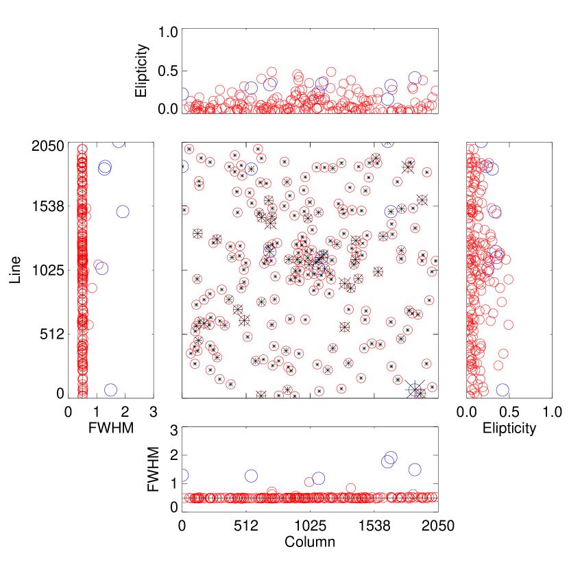
Figure 3: PSF quality assessment of Kron 37 I-band image. The stars are represented by asterisks with sizes proportional to their brightness on the central sky chart. Marginal distributions of the stellar FWHM (left and bottom panels) and ellipticity (right and top panels) are also shown. Stars presenting FWHM above the median value are represented by the bigger blue circles; all the other ones are marked with smaller red circles.

4.3 Performance: SAMI vs SOI

The members of the VISCACHA project have been acquiring SOAR data for a long time. Before the commissioning of the SAM imager, we have extensively used the previous generation imager SOI, establishing a considerable expertise with the instrument. The migration to the new imager after 2013, was an obvious choice given its performance increase over the older instrument.

Therefore, we compare the performance of a typical optical imager without AO, such as SOI, with SAMI as we observed the cluster HW20 in the night 27/09/2016 with both instruments. Exposure times were (6$\times$200) s in the $V$ filter and (6$\times$300) s in $I$ filter. Although the Differential Image Motion Monitor (DIMM) reported a $0.85\arcsec$ seeing for the observations, the SOI $I$ image attained a stellar FWHM of $1.19\arcsec$ and the SAM image reached FWHM of $0.44\arcsec$ on closed loop. Fig. 4 compares a section of the SAM and SOI $I$ images around the centre of HW20 and shows how the decrease of the seeing by the AO system reduces the crowding and effectively improves the depth of the image.

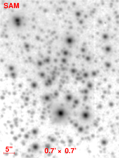
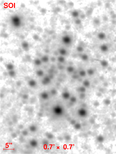
Figure 4: $I$ filter images of the centre of HW20 taken with SAM in closed loop (left panel) and with SOI (right panel) under comparable conditions. The stellar FWHM in the images are 0.44″and 1.19″respectively.

In addition, SOI presents relatively intense fringing in the $I$ filter, requiring correction for precision photometry. Since fringe correction requires at least a dozen dithered exposures of non-crowded fields, we have used a fringe pattern image we derived from 2012B data to correct the fringes in HW20. On the other hand, SAMI $I$ images show negligible to null fringing.

Finally, to empirically compare the instruments, we have performed PSF photometry (see Sect. 4.2) in the fringe-corrected SOI images and SAM images of HW20, subject to the same constraints and relative detection thresholds. Given the different fields of view of these instruments, we have restricted the analysis to an area of $3\arcmin\times 3\arcmin$ near the cluster centre, equally sampled by both instruments. Fig. 5 compares the photometric errors and depth reached by each instrument. It can be seen that with the AO system working at its best, SAM images reach more than one magnitude deeper than SOI under the same sky conditions. Furthermore, the improved resolution also helped detect and deblend more than twice the number of sources found by SOI, particularly in the fainter regime ($I\geq 22.0$).

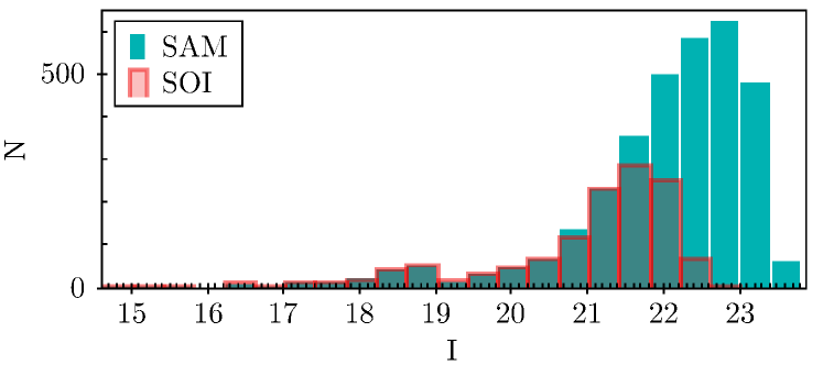
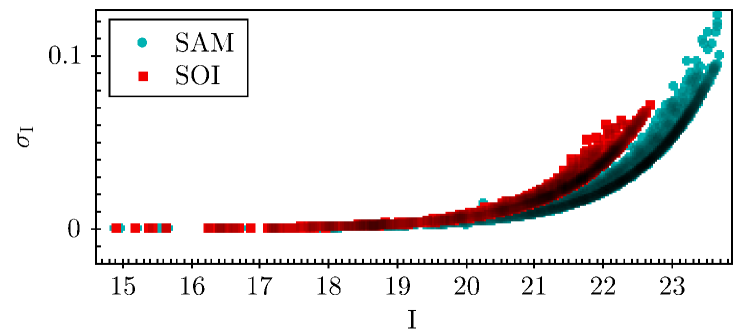
Figure 5: Comparison between SOI and SAM photometry of the HW20 cluster in the $I$ filter, showing the detected objects (top panel) and photometric errors (bottom panel) as function of magnitude. Under the same conditions SAM exposure reaches about 1.2 mag deeper on a photometric night.

4.4 Calibration

Transformation of the instrumental magnitudes to the standard system was done using at least two populous photometric standard fields from Stetson (2000) (e.g. SN1987A, NGC1904, NGC2298, NGC2818), observed at 2 to 4 different airmass through each night. Following the suggestions given in Landolt (2007), the calibration coefficients derived from these fields were calculated in a two-step process:

1. airmass ($X_{j}$), instrumental ($m_{j}$) and catalogue ($M_{j}$) magnitudes in each band ($j$) were employed in a linear fit given by Eq. 1 to evaluate the extinction coefficients ($e_{j}$);

   $$m_{j}-M_{j}=cte+e_{j}X_{j}\quad;$$ (1)

2. the extra-atmospheric magnitudes ($m_{j}^{\prime}=m_{j}-e_{j}X_{j}$) were then used to derive colour transformation coefficients ($c_{j}$) and zero-point coefficients ($z_{j}$) according to Eq. ii):

   $$v^{\prime}-V = z_{v}+c_{v}(V-I)$$

   $$(b^{\prime}-v^{\prime})-(B-V) = z_{bv}+c_{bv}(B-V)$$ (2)

   $$(v^{\prime}-i^{\prime})-(V-I) = z_{vi}+c_{vi}(V-I)$$

Figure 6 shows the fit of Eqs. 1 and ii) to determine the $V$ filter extinction, zero-point and colour coefficients for stars in the NGC2818 and NGC2298 standard fields in the night of February 22, 2015. Since the stars in each standard field were observed more than once (typically at 3 different airmass), the fit of Eq. 1 was made in a star-by-star basis and the final extinction coefficient and its uncertainty determined from the average and deviation of the slopes found. This approach offers a better precision than a single global fitting (i.e. carried out over all stars simultaneously) such as done by iraf, because the intrinsic brightness difference between the standard stars (i.e. the spread in the $y-$axis on the upper panel) is factored out. On the other hand, the colour and zero-point coefficients were found from a global solution using the extra-atmospheric magnitudes for all stars in the two standard fields by means of a robust linear fitting method. At this point, the combination of several standard fields in a single fit is advantageous as it provides a larger sample and wider colour range to help constrain the fit. These fitting procedures were applied to the data calibration from 18 nights observed through semesters 2015A$-$2016B, resulting in the mean coefficient values and deviations shown in Table 3. These values are in excellent agreement with those reported by Fraga et al. (2013).

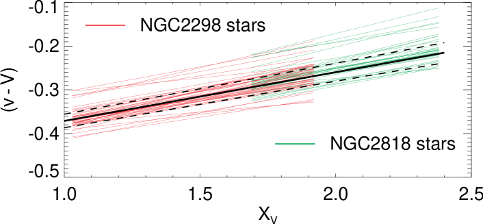
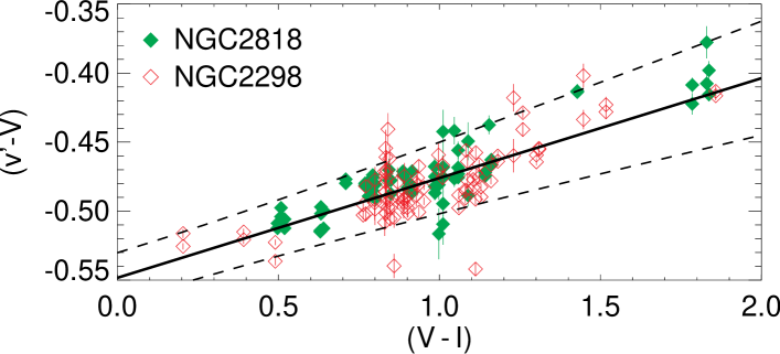
Figure 6: Fits in the $V$ filter to determine the extinction coefficients (top) and the colour and zero-point coefficients (bottom) for the night of 22-02-2015, using the NGC2818 and NGC2298 standard fields. About 70 stars in both fields were used in the determination of the mean extinction coefficient and twice that number in the global fit to determine the colour coefficient. The resulting coefficients and their 6-$\sigma$ uncertainty level are represented by the solid and dashed lines respectively.

Table 3: Mean calibration coefficients through 2015A$-$2016B

Coef.	$B$		$V$		$I$
$e$	$0.177$$\,\pm\,$	$0.011$	$0.106$$\,\pm\,$	$0.006$	$0.022$$\,\pm\,$	$0.006$
$c$	$-0.193$$\,\pm\,$	$0.008$	$0.064$$\,\pm\,$	$0.005$	$-0.063$$\,\pm\,$	$0.005$
$z^{*}$	$-0.138$$\,\pm\,$	$0.006$	$-0.549$$\,\pm\,$	$0.005$	$-0.582$$\,\pm\,$	$0.005$

^∗ relative to the adopted zero point magnitude of 25.

In order to calculate the photometric errors, we first write the colour calibration equations given by Eq. ii) as the following system:

$$\begin{pmatrix}v-e_{v}X_{v}-z_{v}\\ b-v-e_{b}X_{b}+e_{v}X_{v}-z_{bv}\\ v-i-e_{v}X_{v}+e_{i}X_{i}-z_{vi}\end{pmatrix}=\begin{pmatrix}1&0&c_{v}\\ 0&1+c_{bv}&0\\ 0&0&1+c_{vi}\end{pmatrix}\cdot\begin{pmatrix}V\\ B-V\\ V-I\end{pmatrix}$$ (3)

which can be more easily expressed in matrix notation by:

$$\boldsymbol{m}-\boldsymbol{e}-\boldsymbol{z}=\boldsymbol{C}\cdot\boldsymbol{M}\quad,$$ (4)

where the instrumental quantities ($v$, $b-v$, $v-i$) and the corrections due to the zero point ($z$) and extinction ($e$) are now represented by vectors. The calibrated quantities vector ($V$, $B-V$, $V-I$) can be found by inverting this linear system, which requires only calculating the inverse of the colour coefficients matrix ($C$):

$$\boldsymbol{M}=\boldsymbol{C}^{-1}\cdot(\boldsymbol{m}-\boldsymbol{e}-\boldsymbol{z})\quad.$$ (5)

However, propagating the errors through this solution is more subtle, given that the matrix inversion is a nonlinear operation and that the resulting cofactors are often correlated with each other. Following the formalism in Lefebvre et al. (2000), the total uncertainties on the calibrated quantities ($\boldsymbol{\sigma_{M}}$) can be derived analytically from the uncertainties of the instrumental quantities ($\boldsymbol{\sigma_{m}}$), zero point ($\boldsymbol{\sigma_{z}}$), extinction ($\boldsymbol{\sigma_{e}}$) and colour coefficients ($\boldsymbol{\sigma_{C}}$) as:

$$\boldsymbol{\sigma_{M}}^{2}=(\boldsymbol{C}^{-1})^{2}\cdot[\boldsymbol{\sigma_{m}}^{2}+\boldsymbol{\sigma_{e}}^{2}+\boldsymbol{\sigma_{z}}^{2}]\ +\\ +\boldsymbol{\sigma_{C^{-1}}}^{2}\cdot(\boldsymbol{m}-\boldsymbol{e}-\boldsymbol{z})^{2}$$ (6)

where the uncertainties in the inverted colour coefficients matrix ($\boldsymbol{\sigma_{C^{-1}}}$) are calculated directly from the individual colour coefficients uncertainties as:

$$\boldsymbol{\sigma_{C^{-1}}}^{2}=(\boldsymbol{C}^{-1})^{2}\cdot\boldsymbol{\sigma_{C}}^{2}\cdot(\boldsymbol{C}^{-1})^{2}\\ =(\boldsymbol{C}^{-1})^{2}\cdot\begin{pmatrix}0&0&\sigma_{c_{v}}^{2}\\ 0&\sigma_{c_{bv}}^{2}&0\\ 0&0&\sigma_{c_{vi}}^{2}\end{pmatrix}\cdot(\boldsymbol{C}^{-1})^{2}$$ (7)

According to this prescription the total photometric uncertainty of a source, defined by Eq. 6, can be understood as being composed of three components arising from: (i) the PSF photometry (first right hand term), (ii) the extinction correction (second right hand term) and (iii) the colour transformation to the standard system (remaining right hand terms), as shown in Fig. 7. In our data these uncertainties are typically dominated by the extinction correction and colour calibration contributions for stars brighter than $V\sim$19.5, which is about the red clump level of the SMC and LMC clusters, and by the photometric errors for stars fainter than that. Typically, we reached a final error of $\sim$0.1 mag for $V$=24 mag, which is more accurate than those obtained by surveys without the AO system (e.g SMASH, MCPS).

A Monte-Carlo simulation was also employed to propagate the uncertainties through the calibration process. In each step, each coefficient (i.e. zero-point, extinction and colour ones) and instrumental magnitude were individually deviated from its assumed value using a random normal distribution of the respective uncertainty and the calibrated magnitudes calculated through Eq. 5. At the end of $10^{6}$ steps, the standard deviation of each calibrated magnitude was computed and assigned as its total photometric uncertainty. It can be seen in Fig. 7 that the two solutions for propagating the uncertainties are equivalent, with only minor deviations. However, while the Monte-Carlo solution can be computing intensive, the analytical solution presented in Eq. 6 requires negligible computational time.

Figure 7: Photometric uncertainties as function of $V$ for Kron 37. Contributions from the photometry (thin line), the extinction correction (dashed line) and the colour calibration (dotted line) compose the total photometric uncertainty (solid line), which was also derived using a Monte-Carlo simulation (dot-dashed line).

4.5 Completeness

Artificial star tests were performed in each image of the present sample in order to derive completeness levels as function of magnitude and position. The empirical PSF model was used to artificially add stars with a fixed magnitude to the image in a homogeneous grid, with a fixed spacing of 6 FWHM to prevent overlapping of the artificial star wings and overcrowding the field. Several grids with slightly different positioning and with stellar magnitudes ranging from 16 to 25 were simulated, generating more than 100 artificial images for each original one.

Photometry was carried out over the artificial images using the same PSF and detection thresholds as in the original one, and the local recovery fraction of the artificially added stars used to construct spatially resolved completeness maps, as shown in Fig. 8 for Kron 37 at $V=23$mag. It can be seen that incompleteness can severely hamper the analysis of the low mass content of the cluster, as the local completeness value near the centre ($\lesssim 15\%$) falls much more rapidly than the overall field value ($\sim 85\%$). The same trend is clear in Fig. 9 where average completeness curves are shown for three regions: the whole image, the cluster core region and the region outside it. It can be seen that completeness assessments based on an average of the whole image are too optimistic by a factor of 20-50% towards the inner regions of the cluster for stars fainter than the main sequence turnoff level. Usually, the RGB stars have 100% completeness and it starts to decrease from the turnoff towards fainter stars. Because of that we consider the dependence on the magnitude and on the position when applying photometric completeness corrections, before RDP and CMD fitting.

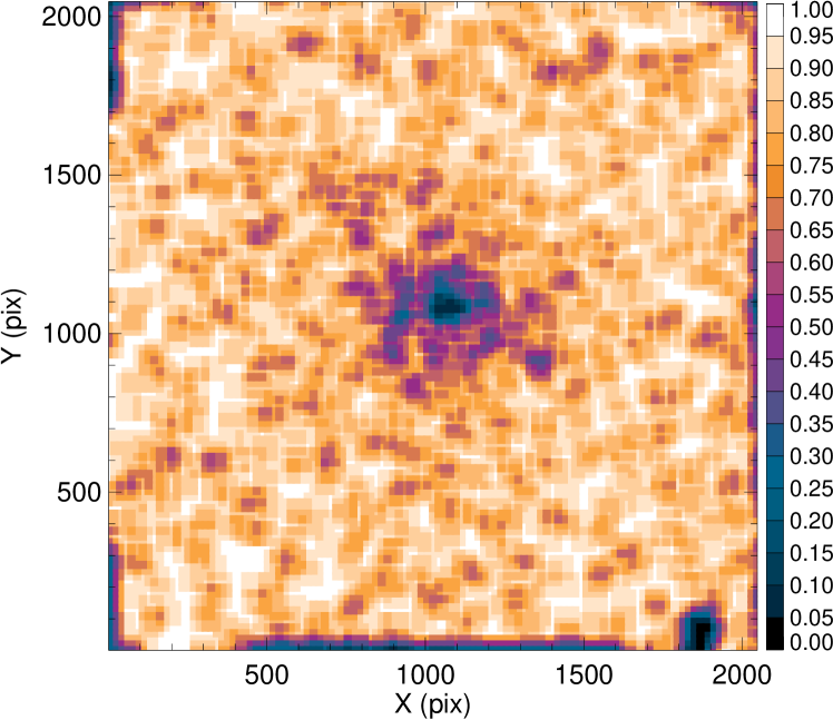
Figure 8: Completeness map for Kron 37, constructed by artificially adding $V=23$ stars over the original image in uniform grids with 6 FWHM spacing, covering the entire image. Even though the average completeness over the image is $\sim$85%, near the centre of the cluster it drops nearly to zero ($<$ 15%).

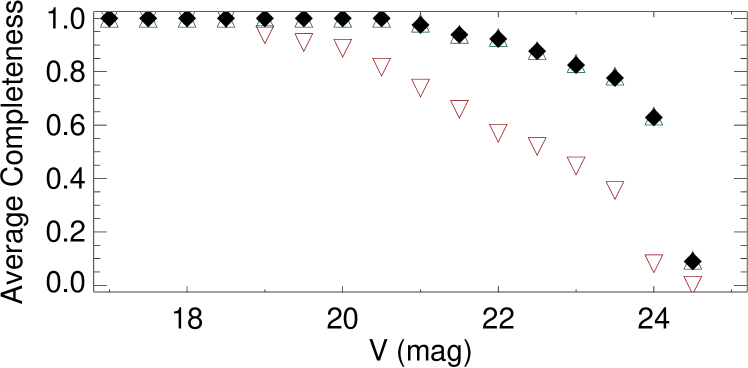
Figure 9: Completeness as a function of $V$ magnitude for Kron 37 over three different regions: the region inside the core radius (down facing red triangles), the one outside it (up facing green triangles) and the whole image (filled black diamonds).

5 Analysis and Methodology

5.1 Radial profile fitting

Given the nature of stellar clusters, it is expected that photometry incompleteness will be higher toward their central regions (see Sect. 4.5). Therefore, if stellar counts are employed to build radial profiles, reliable structural parameters can only be derived after a spatially resolved completeness correction is carried out (e.g. as in Maia et al., 2016; Dias et al., 2016). Alternatively, brightness profiles measured directly over the clusters’ images can also be used (Piatti & Mackey, 2018).

Once a reliable radial profile is built, cluster parameters are usually inferred by fitting an analytic model which describes its stellar distribution. Although the King (1962) model has long been used in describing Galactic clusters, the EFF model (Elson et al., 1987) arguably provides better results for young clusters in the LMC, presenting very large halos. In addition, it has the advantage of also encompassing the Plummer (1911) profile, largely used in simulations.

Nevertheless, we preferred the King (1962) model as it provides a truncation radius to the cluster, effectively defining its size, whereas the EFF model cluster has no such parameter. Also, it generally yields best fits than the EFF model for intermediate-age and old clusters in the Clouds (Werchan & Zaritsky, 2011; Hill & Zaritsky, 2006). We note that dynamical models such as the King (1966) and Wilson (1975) have also been successfully used to describe finite Magellanic Clouds clusters with extended halos (McLaughlin & van der Marel, 2005), being excellent alternatives.

Following this reasoning we have adopted two methods to infer the structural parameters of the present sample. First, surface brightness profiles (SBPs) were derived directly from the calibrated $V$ and $I$ images. Stellar positions and fluxes were extracted from the reduced frames using DAOPHOT (Stetson, 1987), considering only sources brighter than 3 $\sigma$ above the sky level. The centre was then determined iteratively by the stars’ coordinates centroid within a visual radius, starting with an initial guess and adjusted for the new centre at each step. Thereafter, the flux median and dispersion were calculated from the total flux measured in eight sectors per annular bin around this centre. The sky level, obtained from the whole image, was subtracted before the fitting procedure. Although the $I$ band provides the best image quality compared with the $V$ band, its enhanced background makes the resulting profiles noisier. Since smaller uncertainties were achieved for the $V$ band, it was the one used in the present analysis.

The King model (King, 1962) parameters — central surface brightness ($\mu_{0}$), core radius ($r_{c}$) and tidal radius ($r_{t}$) — were estimated by fitting the following function to the SBPs:

$$\mu(r)=\mu^{\prime}_{0}+5\log\left[\frac{1}{\sqrt{1+(r/r_{c})^{2}}}-\frac{1}{\sqrt{1+(r_{t}/r_{c})^{2}}}\right]$$ (8)

where

$$\mu^{\prime}_{0}=\mu_{0}+5\log\left[1-\frac{1}{\sqrt{1+(r_{t}/r_{c})^{2}}}\right].$$ (9)

The fitting range was restricted to the cluster limiting radius, defined as the point where the flux profile reaches an approximately constant level. From the limiting radius outward, the flux measurements were used to compute the stellar background/foreground, which was subtracted from the profile before fitting. There were cases for which it was not possible to obtain $r_{t}$ because background fluctuations dominate the outer profile. Fig. 10 (top panel) shows the fit of Eq. 8 to the SBP of Kron 37. The results for the other clusters in our sample can be found in the appendix (Figs. 14 and 16).

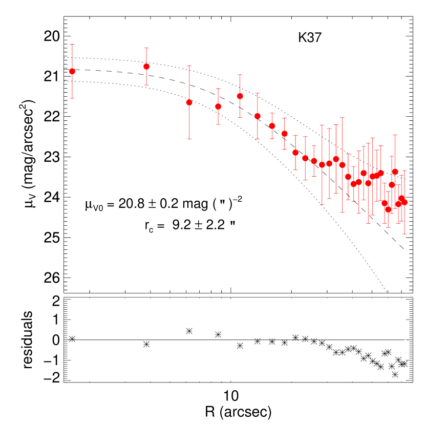
Figure 10: Top panel: fit to the SBP of Kron 37 in the $V$ band along with the residuals of the fit (bottom sub-panel) and the derived parameters: $\mu_{0}$, $r_{c}$ and $r_{t}$. Bottom panel: fit to the completeness corrected stellar density profile of Kron 37 (filled diamonds), for the determination of the parameters $\rho_{0}$, $r_{c}$ and $r_{t}$. Residuals of the fit (bottom sub-panel) and the RDP prior to the completeness correction (open diamonds) are also shown.

As a second approach, we have derived the clusters structural parameters from classical radial density profiles (RDPs) built from completeness corrected stellar counts (e.g Maia et al., 2016), using the King analytical profile:

$$\rho(r)=\rho_{0}\left[\frac{1}{\sqrt{1+(r/r_{c})^{2}}}-\frac{1}{\sqrt{1+(r_{t}/r_{c})^{2}}}\right]^{2}+\rho_{\mathrm{bg}}.$$ (10)

Four different bin sizes were used to build the density profile, keeping the smallest bin size at about the cluster core radius. The fit for Kron 37 is shown in Fig. 10 (bottom panel). It should be noted that a radial profile without any completeness correction (open diamonds) also fits a King profile perfectly well. Although the fit converges, the results obtained are not astrophysically meaningful; the tidal radii can be recovered because incompleteness is not severe there, but the core radii are always in error, usually overestimated by a factor of 2 or higher. The fits for the remaining clusters are shown in Figs. 15 and 17.

The SBP and the RDP are complementary measurements of cluster structure. While SBPs are less sensitive to incompleteness than RDPs, a critical issue towards the clusters’ centre, stochasticity and heterogeneity of field stars towards the outer cluster regions make the fluctuations on the SBP background much higher than those of the RDP background. Even if this can hinder or even make impossible the determination of the tidal radius in SBPs, the problem is mitigated in the RDPs, allowing reliable determination of this parameter even without completeness correction.

While the SBP uncertainties grow from the cluster centre to its periphery due to progressive flux depletion, the RDP uncertainties decrease in this sense as a consequence of the steadily rise of the number of stars. By combining the structural parameters obtained from King (1962) model fitting to the SBP and to the RDP of the clusters, we expect to minimize such uncertainties across the entire profile. The parameters’ weighted average and uncertainty were calculated as:

$$\bar{x}=\dfrac{\sum(x_{i}/\sigma_{i}^{2})}{\sum(1/\sigma_{i}^{2})},$$

$$\sigma_{\bar{x}}=\sqrt{\dfrac{1}{\sum(1/\sigma_{i}^{2})}}.$$

The tidal radii of the clusters K 37, HW 20 and KMHK 228 come only from the RDP because their fits did not converge for the SBP. Based on the resulting $r_{c}$ and $r_{t}$ values, the clusters concentration parameter $c\equiv\log{(r_{t}/r_{c})}$ (King, 1962) was also derived. Table 4 compiles the resulting structural parameters for the present clusters.

Table 4: Structural parameters of target clusters

Name	RA	Dec	$\mu_{0}$	$r_{c}$		$r_{t}$		$c$		$\sigma_{\mathrm{bg}}$
	[h:m:s]	[ ∘ : $\arcmin$ : $\arcsec$ ]	[mag$\cdot$arcsec-2]	[arcsec]		[arcsec]				[$10^{-3}\cdot$arcsec-2]
AM3	23:48:59	-72:56:43	22.7$\pm$0.3	5.6$\pm$	0.8	54$\pm$	8	0.9$\pm$	0.1	1.0$\pm$	0.1
HW20	00:44:47	-74:21:46	22.6$\pm$0.3	10.8$\pm$	2.0	37$\pm$	11	0.5$\pm$	0.2	30.7$\pm$	9.5
K37	00:57:47	-74:19:36	20.8$\pm$0.2	11.3$\pm$	1.5	83$\pm$	17	0.8$\pm$	0.1	23.6$\pm$	6.7
NGC796	01:56:44	-74:13:10	18.4$\pm$0.3	3.2$\pm$	0.5	97$\pm$	9	1.2$\pm$	0.1	1.5$\pm$	0.5
KMHK228	04:53:03	-74:00:14	23.8$\pm$0.4	19.8$\pm$	5.9	68$\pm$	16	0.6$\pm$	0.2	25.6$\pm$	2.9
OHSC3	04:56:36	-75:14:29	19.4$\pm$0.7	4.3$\pm$	0.7	42$\pm$	6	0.9$\pm$	0.1	12.9$\pm$	3.7
SL576	05:33:13	-74:22:08	20.0$\pm$0.2	10.6$\pm$	1.3	43$\pm$	5	0.6$\pm$	0.1	30$\pm$	14
SL61	04:50:45	-75:31:59	22.1$\pm$0.2	26.5$\pm$	2.6	162$\pm$	44	0.8$\pm$	0.2	0.1$\pm$	6.2
SL897	06:33:01	-71:07:40	21.2$\pm$0.2	12.0$\pm$	1.7	87$\pm$	9	0.9$\pm$	0.1	2.8$\pm$	0.9

5.2 Isochrone fitting

For the analysis of the photometric data, we initially used the structural parameters to define the cluster and field samples within each observed field. Usually all stars inside the cluster tidal radius were assigned to the cluster sample and the ones outside it to the field sample. For a few clusters presenting $r_{t}$ close to or larger than the image boundaries (i.e. leaving no field sample), half the tidal radius was employed as a cluster limit instead. Integration of the King profiles have shown that depending on the concentration parameter, 75% ($c\sim$ 0.5) to 99% ($c\gtrsim$ 1.0) of the cluster population lies within that radius, ensuring sufficient source counts in both cluster and field samples. The implications of this choice are discussed and accounted for in Sect 5.3. Then, a decontamination procedure (Maia et al., 2010) was applied to statistically probe and remove the most probable field contaminants from the cluster region, based on both the positional and the photometric characteristics of the stars, comparing the cluster and field regions defined above.

The field decontaminated CMD of the clusters were then used to derive their astrophysical parameters via the Markov-Chain Monte-Carlo technique in a Bayesian framework. The likelihood function was derived using PARSEC isochrones (Bressan et al., 2012) to build synthetic CMDs of simple stellar populations, spanning a wide range of parameters (e.g. Dias et al., 2014). Figure 11 shows the posterior distribution of the determined parameters for Kron 37. Typical uncertainties of the method are about $0.15$ dex in metallicity, $10$-$20\%$ in age, $\sim$2 kpc in distance and $\sim$0.02 mag in colour excess. Figure 12 shows the best model isochrone and the synthetic population superimposed over the Kron 37 decontaminated CMD. Respective figures for all other SMC and LMC clusters can be found in Appendix B.

The distance estimates were used to convert the core and tidal radii previously derived in Sect. 5.1 to physical sizes, thus allowing a more meaningful comparison of their values. Most of our targets present core sizes of 2-3 pc, with the exceptions of NGC796 and OHSC3 which showed more compact cores and SL61 presenting a very inflated one. Tidal sizes were mainly found in the range of 10-20 pc, except for K37, NGC796 and SL61, presenting larger tidal domains. Table 5 compiles the resulting astrophysical parameters.

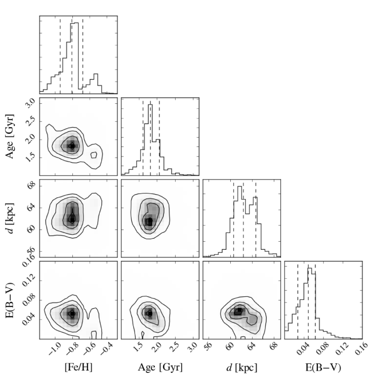
Figure 11: Posterior distribution of parameters derived for Kron 37 using a MCMC bayesian framework. The derived parameters and their uncertainties are also shown.

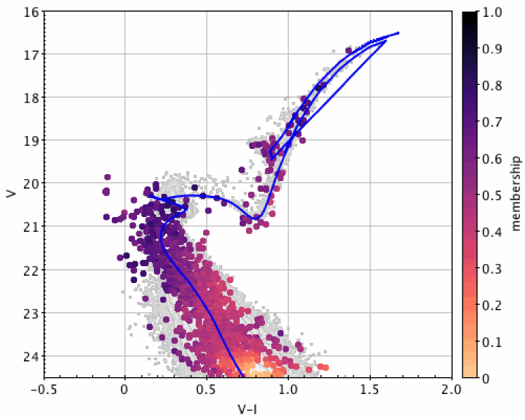
Figure 12: Best model isochrone (solid line) and synthetic population (gray dots) corresponding to the Kron 37 parameters, superimposed over its field decontaminated CMD.

Table 5: Astrophysical parameters from isochrone and mass function fits.

Name	galaxy	$r_{c}$	$r_{t}$	Age	[Fe/H]	E(B-V)	dist.	Mobs	Mint	$\alpha$
		[pc]	[pc]	[Gyr]			[kpc]	[103 M⊙]	[103 M⊙]
AM3	SMC	1.76$\pm$0.26	17.0$\pm$2.6	$5.48^{+0.46}_{-0.74}$	$-1.36^{+0.31}_{-0.25}$	$0.06^{+0.01}_{-0.02}$	$64.8^{+2.1}_{-2.0}$	0.23$\pm$0.05	$--$	$-$0.27$\pm$0.98
HW20	SMC	3.26$\pm$0.61	11.2$\pm$3.3	$1.10^{+0.08}_{-0.14}$	$-0.55^{+0.13}_{-0.10}$	$0.07^{+0.02}_{-0.01}$	$62.2^{+2.5}_{-1.2}$	0.56$\pm$0.10	2.06$\pm$0.43	$-$2.51$\pm$0.61
K37	SMC	3.42$\pm$0.47	25.1$\pm$5.2	$1.81^{+0.24}_{-0.21}$	$-0.81^{+0.13}_{-0.14}$	$0.05^{+0.01}_{-0.02}$	$62.4^{+2.3}_{-1.8}$	2.58$\pm$0.19	9.20$\pm$2.03	$-$1.97$\pm$0.22
NGC796	Bridge	0.94$\pm$0.15	28.4$\pm$2.9	$0.04^{+0.01}_{-0.02}$	$-0.31^{+0.09}_{-0.12}$	$0.02^{+0.01}_{-0.01}$	$60.3^{+2.7}_{-2.4}$	1.12$\pm$0.22	3.60$\pm$0.70	$-$2.31$\pm$0.17
KMHK228	LMC	5.8$\pm$1.7	19.8$\pm$4.7	$0.88^{+0.33}_{-0.16}$	$-0.20^{+0.06}_{-0.06}$	$0.05^{+0.03}_{-0.01}$	$60.0^{+1.9}_{-2.4}$	0.23$\pm$0.05	1.35$\pm$0.30	$-$2.48$\pm$0.52
OHSC3	LMC	1.01$\pm$0.17	9.8$\pm$1.5	$1.79^{+0.22}_{-0.20}$	$-0.70^{+0.13}_{-0.24}$	$0.07^{+0.02}_{-0.02}$	$48.3^{+2.0}_{-1.8}$	0.44$\pm$0.10	$--$	$-$1.18$\pm$0.45
SL576	LMC	2.64$\pm$0.34	10.7$\pm$1.3	$0.97^{+0.10}_{-0.11}$	$-0.39^{+0.08}_{-0.12}$	$0.02^{+0.03}_{-0.01}$	$51.3^{+1.9}_{-2.4}$	1.81$\pm$0.22	5.83$\pm$1.09	$-$2.14$\pm$0.39
SL61	LMC	6.55$\pm$0.68	40$\pm$11	$2.08^{+0.27}_{-0.21}$	$-0.44^{+0.14}_{-0.19}$	$0.10^{+0.02}_{-0.02}$	$51.0^{+1.5}_{-1.7}$	3.02$\pm$0.25	7.00$\pm$1.19	$-$1.72$\pm$0.30
SL897	LMC	2.65$\pm$0.39	19.2$\pm$2.2	$1.19^{+0.14}_{-0.12}$	$-0.32^{+0.11}_{-0.14}$	$0.09^{+0.02}_{-0.02}$	$45.6^{+2.4}_{-1.6}$	1.17$\pm$0.14	5.11$\pm$1.07	$-$2.49$\pm$0.36

5.3 Stellar mass function fitting

The distribution of mass in a stellar cluster can yield important information on its evolutionary state and on the external environment. As none of the studied objects show any sign of their pre-natal dust or gas given their ages, their stellar components are the only source of their gravitational potential (e.g. Lada & Lada, 2003). Thus, the number of member stars and their concentration will determine, in addition to the galaxy potential, for how long clusters survive.

To derive the stellar mass distribution of the target clusters, a completeness corrected $M_{I}$ luminosity function (LF) was first built by applying the distance modulus and extinction corrections to the stars’ magnitudes. Afterwards, the LF was converted to a mass function (MF) employing the mass-$M_{I}$ relation from the clusters’ best-fitted model isochrone, using the procedure described in Maia et al. (2014). The observed cluster mass ($M_{\mathrm{obs}}$) is then obtained by adding up the contributions of individual bins across the MF.

The MF slope was determined by fitting a power law over the cluster mass distribution. Following the commonly used notation, our power law can be written as:

$$\xi(m)=\frac{dN}{dm}=Am^{\alpha},$$ (11)

where $\alpha$ is the MF slope and $A$ is a normalisation constant. To avoid discontinuities and multiple values in the $M_{I}$-mass relationships, the MF slope fitting procedure was restricted to main sequence stars, thus excluding giants beyond the turn-off. The masses and the stellar MF slopes obtained for all clusters are shown in Table 5.

Fig. 13 shows the luminosity function, the resulting mass function and the fit of Eq. 11 for Kron 37. Figs. 20 and 21 show the resulting LF and MF for the remaining samples clusters. We typically reach stellar masses as low as 0.8 $M_{\odot}$ under good AO performance, and about 1.0 $M_{\odot}$ otherwise. This limit is deeper than that reached by large surveys in the crowded regions of star clusters (e.g. MCPS will reach $\sim$2.5 $M_{\odot}$ at 50% completeness level for a typical main sequence star in the SMC). We note that the spatially resolved completeness correction employed is crucial in probing the low-mass regime.

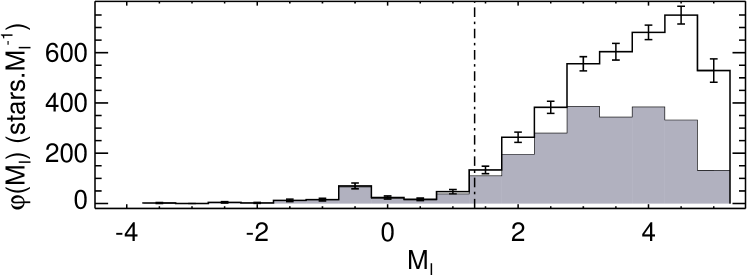
Figure 13: Top panel: $M_{I}$ luminosity function for Kron 37 built with the observed (filled histogram) and completeness corrected (open histogram) samples. Bottom panel: resulting mass function of Kron 37 from observed (open symbols) and completeness corrected (filled symbols) samples. The turn-off magnitude and mass are indicated by a vertical dashed line and the best fitting power-law is represented by the solid line. Total observed mass and resulting MF slope are also indicated.

Whenever it could be assumed that a cluster stellar content follows the IMF, i.e. it presents a (high mass) MF slope that is compatible with the expected value of $\alpha=-2.30\pm 0.36$ given by Kroupa et al. (2013), its total mass was estimated by integrating this analytical IMF down to the theoretical mass limit of 0.08 M_⊙. Uncertainties on the IMF analytical parameters and the normalization constant $A$, derived in the MF fit, were properly propagated into the total integrated mass (M_int), shown in Table 5.

Since clusters K37, NGC796, SL61 and SL897 presented sizes ($r_{t}$) outside or very close to the image boundaries, their mass functions were estimated using only stars inside their inner region (within half $r_{t}$). Their total observed masses were later corrected to their full spatial extent based on integrations of their King profiles. Given the way the stars are distributed in each cluster, the correction factors amounted to 1.01-1.35, being higher for less concentrated clusters like SL61 and almost negligible to the concentrated ones like NGC796.

This was also reflected on the MF slope of these two clusters, which were found slightly flatter than the IMF, indicating a deficit of low mass content in their inner region. This could be interpreted as a sign of mass segregation or preferential loss of the low mass content, depending on whether these stars are found in the periphery of these clusters or not. Both hypotheses have implications regarding the clusters dynamical evolution and the external tidal field acting on them.

Similarly, AM3 and OHSC3 presented MF slopes significantly flatter than expected by the IMF. Since their full extent was sampled by the images, it is possible to assert that severe depletion of their lower mass content took place. Their low mass budget and advanced ages makes them specially susceptible to stellar evaporation and tidal stripping effects. The remaining clusters showed no such signs of depletion of their stellar content.

In most cases the total integrated mass is 2-4 times the observable mass of the cluster. This can be explained by the shape of the IMF which peaks around 0.5 M_⊙, below the minimum observed mass of $\sim$0.8–1.0 M_⊙, implying that most of the cluster mass lies in the less massive stellar content, unseen by our observations. The errors of the integrated masses are larger than those of the observed masses because they include (and are dominated by) the uncertainty in the exponents of the adopted IMF (Kroupa et al., 2013) in this lower mass regime.

6 First Results

Tables 4 and 5 summarize the parameters determined for a sample of 9 clusters from the present data set. These were chosen to represent the large variety of cluster types found, in terms of richness, ages, metal content and density. In this section, we discuss our results in comparison with those provided in the literature. Many clusters had their ages previously derived from integrated photometry and ours are the first estimates based on stellar isochrone fitting. Similarly, distances and/or metallicities were often assumed constant in previous photometric studies, making our values the first set of simultaneously derived, self-consistent parameters. In addition, determinations of most of the clusters’ mass budgets and mass distributions were done for the first time in this work. Particularly, we derived for the first time the considered astrophysical parameters for HW20 and KMHK228. We discuss below the results for each cluster and compare them with the available literature.

OHSC 3 (LMC)

From integrated spectroscopy, Dutra et al. (2001) obtained an age of 1-2 Gyr for OHSC 3, in agreement with our determination, and reddening $E(B-V)$=0.12 from Schlegel et al. (1998) dust maps, a little over our estimate from isochrone fitting.

SL 576 (LMC)

Bica et al. (1996) derived for SL 576 an age in the range 200-400 Myr from the measured integrated colours ($U-B$)=0.08 and ($B-V$)=0.38 and their calibration with Searle et al. (1980) SWB type. Our analysis gave an age consistent with a much older cluster (0.97 Gyr). Integrated colours may be affected by stochastic effects from bright field stars superimposed on the cluster direction, specifically in this case a non-member blue star would contribute to lower the cluster integrated colours, and so mimicking a younger cluster. On the other hand, in our photometry this issue was accounted for with the decontamination procedure where any outsider is excluded before the isochrone fitting.

SL 61 (LMC)

Among the LMC clusters in our sample, SL 61 (=LW 79) is the most studied. Geisler et al. (1997) determined an age of 1.8 Gyr by measuring the magnitude difference between main sequence turnoff and red clump and using a calibration of this parameter with age. Its integrated colours, ($U-B$)=0.27 and ($B-V$)=0.59, place SL 61 in the age range 0.6-2.0 Gyr (Girardi et al., 1995; Bica et al., 1996). By adopting ($m-M$)_∘ = 18.31 and $E(B-V)$ = 0.08 from independent measurements, Mateo (1988) performed isochrone fits to the clusters’ cleaned CMD built from $BVR$ photometry (Mateo & Hodge, 1987), obtaining [Fe/H]=0.0 and an age of 1.8 Gyr or 1.5 Gyr depending on the stellar models used, with or without overshooting, respectively. Grocholski et al. (2007) redetermined an age of 1.5 Gyr based on the cluster photometry by Mateo & Hodge (1987) and updated isochrones. Using the red clump $K$ magnitude, they obtained a distance of $49.9\pm 2.1$ kpc, and considering Burstein & Heiles (1982) extinction maps, a reddening of $E(B-V)=0.11$ was adopted. From a calibration of the Ca II triplet with metallicity, Grocholski et al. (2006) derived [Fe/H]$=-0.35\pm 0.04$ from 8 stars and Olszewski et al. (1991), using the same technique, obtained [Fe/H]=-0.50 based on a single cluster star. In general, our results are in agreement with those of the literature, which are compatible among themselves. Regarding the cluster age, our value (2.08 Gyr) is consistent with literature upper estimates given the uncertainties quoted in Table 5. Since our deep photometry resolves stars some magnitudes below the turnoff, we are confident of the age derived, because the CMD region most sensitive to age was assessed and thus a reliable isochrone match was possible. Our derived metallicity is intermediate between those determined from Ca II triplet spectra. The same conclusion can be drawn for the reddening and distance derived.

SL 897 (LMC)

Integrated photometry of SL 897 (=LW 483) yielded colours ($U-B$)=0.24 and ($B-V$)=0.56, that are compatible with an intermediate-age (400-800 Myr) cluster (Bica et al., 1996). Piatti & Bastian (2016) investigated the cluster by means of $gi$ photometry using the 8-m Gemini-S telescope obtaining a deep, high quality CMD. Isochrone fits to a cleaned CMD determined an age of $1.25\pm 0.15$ Gyr by adopting initial values of metallicity ([Fe/H]=-0.4), reddening ($E(B-V)$=0.075) and distance modulus (($m-M$)${}_{\circ}=18.49\pm 0.09$) from previous observational constraints. Recalling that in our analysis all parameters were free in the search for the best solution, we found similar age, metallicity and reddening (see Table 5). As for the distance, our study places the cluster closer than the LMC average, the value used by Piatti & Bastian (2016).

This is also the only cluster in our LMC sample that had its structural properties previously investigated, allowing a direct comparison with our results. Piatti & Bastian (2016) derived $r_{c}=2.7\pm 0.5$ pc and $r_{t}=36.4\pm 2.4$ pc from star counts. While our determined core radius is similar ($r_{c}=2.6\pm 0.4$ pc), our tidal radius ($r_{t}=19.2\pm 2.2$ pc) is considerably smaller, but comparable to their value for the cluster radius ($r_{cls}=21.8\pm 1.2$ pc). Besides the distance difference, we identified two possible reasons for this discrepancy: (i) while Piatti & Bastian (2016) RDP extends to $\sim 160\,\arcsec$, ours is restricted to $\sim 80\,\arcsec$ and (ii) their photometry being slightly deeper, it may catch lower mass stars which occupy cluster peripheral regions as a consequence of evaporation and mass segregation. We postpone a detailed analysis of this issue for a forthcoming paper dealing with structural parameters of VISCACHA clusters.

KMHK 228 (LMC)

For KMHK 228 we provide astrophysical parameters for the first time.

AM 3 (SMC)

This is one of the three clusters discovered by Madore & Arp (1979) who indicated it as the possible westernmost cluster of the SMC. It is also in the west halo group classified by Dias et al. (2014). The reddening was derived only by Dias et al. (2014) as E(B-V)=0.08$\pm$0.05 which agrees very well with our derived value of E(B-V)=0.06${}^{+0.01}_{-0.02}$. Distance was only derived by Dias et al. (2014) as 63.1${}^{+1.8}_{-1.7}$ kpc in good agreement with our result of 64.8${}^{+2.1}_{-2.0}$ kpc. The age of AM 3 was derived by Dias et al. (2014) as 4.9${}^{+2.1}_{-1.5}$ Gyr, and also by Piatti & Perren (2015); Piatti (2011); Da Costa (1999) as 4.5$\pm$0.7 Gyr, 6.0$\pm$1.0 Gyr, and 5-6 Gyr respectively, but the last three fixed distance and reddening values to derive the age. Nevertheless all age estimates agree with ours of 5.5${}^{+0.5}_{-0.7}$ Gyr. Metallicity was only derived from photometry so far: [Fe/H] = -0.75$\pm$0.40, -0.8${}^{+0.2}_{-0.6}$, -1.25$\pm$0.25, -1.0 by Piatti & Perren (2015); Dias et al. (2014); Piatti (2011); Da Costa (1999) respectively, and now we derived [Fe/H] = -1.36${}^{+0.31}_{-0.25}$. This rather large uncertainty in metallicity is owing to the low number of RGB stars to properly trace its slope. We are carrying out a spectroscopic follow-up to better constrain the AM3 metallicity.

The structural parameters were only derived by Dias et al. (2014): $r_{c}=18.1\pm 1.1\arcsec$ and $r_{t}=62\pm 6\arcsec$. The tidal radius agrees with our value of $r_{t}=54\pm 8\arcsec$ and with the estimated size of 0.9$\arcmin$ from the Bica catalogue (Bica & Schmitt, 1995). The core radius is larger than that derived by us, $r_{c}=5.6\pm 0.8\arcsec$. The difference comes from the unresolved stars in the centre of the cluster using SOI photometry by Dias et al. (2014), who derived only the RDP and were limited by some bright stars in the inner region. We could resolve the central stars using AO with SAMI and we confirmed the core radius using the SBP. Da Costa (1999) estimated M${}_{\rm V}=-3.5\pm 0.5$ mag as the total luminosity of AM 3, which corresponds to M$\sim 2.5\times 10^{3}$M_⊙. We refrained from calculating a total integrated mass for AM3, given that its MF slope showed heavy depletion of its lower mass stellar content. This behavior implies a smaller contribution from the unseen low mass content, meaning that its integrated mass would be closer to the observed mass budget.

HW 20 (SMC)

This cluster belongs to the wing/bridge group in the classification of Dias et al. (2014). We derive accurate age, metallicity, distance, and reddening for the first time and found 1.10${}^{+0.08}_{-0.14}$ Gyr, [Fe/H] = -0.55${}^{+0.13}_{-0.10}$, E(B-V) = 0.07${}^{+0.02}_{-0.01}$, d = 62.2${}^{+2.5}_{-1.2}$ kpc. The only previous estimatives of age and metallicity were done by Rafelski & Zaritsky (2005) fitting integrated colours to two models and different metallicities. The combination with smaller error bars is using STARBURST: [Fe/H] $\approx$ -1.3 and age 5.7${}^{+0.8}_{-4.3}$ Gyr, which is very different from our determinations. Another combination agrees better with our results but with larger error bars using GALEV: [Fe/H] $\approx$ -0.7, age 1.2${}^{+9.1}_{-0.5}$ Gyr.

The structural parameters were derived before by Hill & Zaritsky (2006): $r_{c}=3.05$ pc and the 90% light radius as 18.28 pc. The core radius agrees well with our determination of $r_{c}=3.26\pm 0.61$ pc, but their 90% radius is significantly larger than the tidal radius derived here: $r_{t}=11.2\pm 3.3$ pc. The size estimated in the Bica catalogue (Bica & Schmitt, 1995) of 0.75$\arcmin$ agrees better with our tidal radius of 37$\pm$11$\arcsec$. Hill & Zaritsky (2006) used photometry from the MCPS that is limited to $V<21$ mag while we included also fainter stars down to $V<24$ mag. Figs. 16 and 17 show that the sky background is high, and that a tidal radius much larger than 11-12$\arcsec$ would not fit the profile. It is possible that the fitting by Hill & Zaritsky (2006) was limited by a poor determination of the sky background based only on bright stars in a crowded region. Rafelski & Zaritsky (2005); Hill & Zaritsky (2006) derived $M_{\rm V}$ = 14.97 and 16.2, which corresponds to $M\sim$ 4.3$\times 10^{3}$M_⊙ and $\sim$ 1.2$\times 10^{3}M_{\odot}$. Our mass determination is within this range: $M=2.06\pm 0.43\times 10^{3}M_{\odot}$.

K 37 (SMC)

This is also a wing/bridge cluster in the classification of Dias et al. (2014). SIMBAD classifies it as an open Galactic cluster, but based on its position and distance, it is probably an SMC cluster. Accurate age was derived only by Piatti (2011) as 2.0$\pm$0.3 Gyr based on the magnitude difference between MSTO and RC. Glatt et al. (2010) estimated $\sim$1.0 Gyr with error bars larger than 1-2 Gyr based on MCPS photometry that is limited to clusters younger than 1 Gyr. Rafelski & Zaritsky (2005) derived ages based on integrated colours, and the combination of model, metallicity, and age with smaller error bars led to an age of 1.13${}^{+0.05}_{-0.10}$ Gyr for a metallicity of [Fe/H] $\sim$ -0.7. Accurate spectroscopic metallicity was derived by Parisi et al. (2015) as [Fe/H] = -0.79$\pm$0.11 based on CaII triplet lines. Piatti (2011) derived [Fe/H] = -0.90$\pm$0.25 based on the RGB slope. Although both values agree with ours [Fe/H] = -0.81${}^{+0.13}_{-0.14}$ within uncertainties, we call attention to the fact, that the very good agreement with the spectroscopic value gives strength to the VISCACHA metallicities whenever the cluster has enough RGB stars.

The structure parameters from previous works do not agree very well. Hill & Zaritsky (2006) and Kontizas et al. (1985) derived $r_{c}=3.36_{-0.92}^{+2.14}$ pc and $r_{c}=1.3$ pc, respectively, and our result of $r_{c}=3.42\pm 0.47$ pc agrees well with the most recent value. The same authors derived $r_{90}=11.07_{-3.29}^{2.2}$ pc and $r_{t}=40.3$ pc and none of them are close to our derived value of $r_{t}=25.1\pm 5.2$ pc. As the case of HW 20, our photometry is deeper and our images have better spatial resolution, therefore we are not biased by bright stars only as it may be the case of the previous works. In fact, our $r_{t}=83\pm 17\arcsec$ agrees with the cluster size by Piatti (2011) and Bica & Schmitt (1995) of r=70$\pm$10$\arcsec$ and 1.0$\arcmin$, respectively, but not with Glatt et al. (2010) who derived r=0.5$\arcmin$. The difference is probably because of their shallow MCPS photometry. All previous integrated magnitudes agree between M_V=14.1-14.2 (Hill & Zaritsky, 2006; Rafelski & Zaritsky, 2005; Bica et al., 1986; Gascoigne, 1966), which means 9-10$\times 10^{3}$M_⊙, in good agreement with our determination of M=9.2$\pm 2.0\times 10^{3}$M_⊙.

NGC 796 (SMC)

This is another wing/bridge cluster based on the classification of Dias et al. (2014). It is possibly the youngest cluster in the Magellanic Bridge, the only one with an IRAS counterpart, defined by Herbig Ae/Be and OB stars (Nishiyama et al., 2007). Accurate age was derived by Kalari et al. (2018) who observed the cluster in the very same night as we did using SAMI@SOAR, but using griH$\alpha$ filters. They derived 20${}^{+12}_{-5}$ Myr assuming a metallicity of [Fe/H] $<-0.7$. Bica et al. (2015) derived 42${}^{+24}_{-15}$ Myr, which agrees with our determination of 0.04${}^{+0.01}_{-0.02}$ Gyr and with the estimates of a young age based on integrated spectroscopy ranging from 3-50Myr (Santos et al., 1995; Ahumada et al., 2002). The older age derived by Piatti et al. (2007) of 110${}^{+50}_{-20}$ Myr (assuming $d=$56.8 kpc, $E(B-V)=0.03$, [Fe/H] = -0.7 to -0.4) was explained by Bica et al. (2015): their CMD did not include some saturated stars. Metallicity was only derived by Bica et al. (2015) as [Fe/H] = -0.3${}^{+0.2}_{-0.3}$ which agrees very well with our value of [Fe/H] = -0.31${}^{+0.09}_{-0.12}$. Reddening is very similar: 0.03 derived by Ahumada et al. (2002), Bica et al. (2015) and Kalari et al. (2018) in agreement with ours of 0.02${}^{+0.01}_{-0.01}$. The distance derived by Kalari et al. (2018) of 59$\pm$0.8 kpc agrees very well with ours (60.3${}^{+2.7}_{-2.4}$ kpc), and the much closer distance of 40.6$\pm$1.1 kpc derived by Bica et al. (2015) was considered very unlikely by Kalari et al. (2018) based on spectroscopic parallax.

The structural parameters were derived by Kontizas et al. (1986) and Kalari et al. (2018): $(r_{c},r_{t})=(0.2,36.5)$ pc and $(1.4\pm 0.3,13.9\pm 1.2)$ pc, respectively. These values do not agree with each other and our determinations lie in between: $(r_{c},r_{t})=(0.94\pm 0.15,28.4\pm 2.9)$ pc. The photometric quality obtained by Kalari et al. (2018) is very similar to ours, but they used rings of similar density instead of circles around the cluster centre as we did, and they found anomalies in their fit, possibly because of this choice. Another difference is that they fit Elson et al. (1987) profiles and we fit King profiles. Kalari et al. (2018) found an MF slope of $\alpha=-1.99\pm 0.2$, similar to the value we found $\alpha=-2.31\pm 0.17$. Their derived integrated mass of 990$\pm$220 $M_{\odot}$ considered only stars more massive than 0.5 $M_{\odot}$, and used their derived MF slope, which is slightly flatter than ours, for integration. In our experience, the stellar content less massive than 0.5 $M_{\odot}$ usually accounts for roughly half the cluster’s integrated mass budget when it can be assumed to follow the IMF. Correcting for this and for the difference in the MF slopes, their reported mass becomes compatible with ours. The integrated magnitude by Gordon & Kron (1983) of $M_{\rm V}=-0.97\pm 0.03$ mag, meaning $M\sim$ 200 M_⊙, should be taken with caution as the bright stellar content of this young cluster introduces a lot of stochasticity in the integrated magnitudes. Finally the derived mass by Kontizas et al. (1986) of $4\times 10^{3}$ $M_{\odot}$ agrees with our determination of $(3.6\pm 0.7)\times 10^{3}$ $M_{\odot}$.

7 Conclusions and Perspectives

We presented the VISCACHA survey, an observationally homogeneous optical photometric database of star clusters in the Magellanic Clouds, most of them located in their outskirts and having low surface brightness and for this reason largely neglected in the literature. Images of high quality (sub-arcsecond) and depth were collected with adaptive optics at the 4-m SOAR telescope. Our goals are: (i) to investigate Magellanic Cloud regions as yet unexplored with such comprehensive, detailed view, in order to establish a more complete chemical enrichment and dynamical evolutionary scenario for the Clouds, since their peripheral clusters are the best witnesses of the ongoing gravitational interaction among the Clouds and the MW; (ii) to assess relations between cluster structural parameters and astrophysical ones, aiming at studying evolutionary effects on the clusters’ structure associated with the tidal field (location in the galaxy); (iii) to map the outer cluster population of the Clouds and identify chemical enrichment episodes linked to major interaction epochs; (iv) to evaluate the cluster distribution of both galaxies with the purpose of establishing the 3D structures of the SMC and the LMC.

In this first paper, the methods used to explore the cluster properties and their connections with the Clouds were detailed. We have shown that the careful image processing, PSF extraction and calibration methods employed, delivered high quality photometric data, unmatched by previous studies. Furthermore, a detailed spatially resolved completeness treatment allied with a robust analysis methodology proved crucial in deriving corrections to the most commonly used techniques in cluster analysis, such as the ones used to determine density profiles, CMDs and luminosity and mass functions. A reliable and homogeneously derived compilation of astrophysical parameters was provided for a sample of 9 clusters. Enlargement of this sample will allow us to better understand the galactic environment at the Magellanic Clouds periphery and to address our longer term goals.

In future work we intend to present a more detailed analysis of the whole cluster sample on each topic described in this paper, and present more general results concerning both Clouds. Then, we shall study the mass function and possible mass segregation, as well as constrain the star formation and tidal history in both Clouds.

Appendix A Structural analysis charts for studied clusters

This appendix compiles figures resulting from the structural analysis of the studied clusters, as described in Sect. 5.1. Figs. 14 and 16 shows the fits of the King function (Eq. 8) over the surface brightness profiles (SBPs) of studied clusters. Figs. 15 and 17 shows the fits of the King function (Eq. 10) over the radial density profiles (RDPs) of the studied clusters.

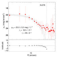
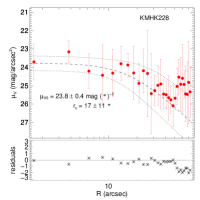
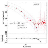
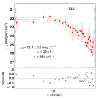
Figure 14: King model fits (dashed lines) with 1-sigma uncertainty (dotted lines) to SBPs (red dots and error bars) of clusters SL576, KHMK228, OHSC3 and SL61 (from top left to bottom right). The lower panel in each plot shows the residuals. The resulting parameters are indicated.

Figure 15: King model fits (dashed lines) with 1-sigma uncertainty (dotted lines) to the original (open symbols) and completeness corrected RDPs (filled symbols) of clusters SL576, KMHK228, OHSC3, SL61 (from top left to bottom right). The lower panel in each plot shows the residuals. The resulting parameters are indicated.

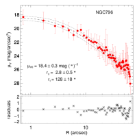
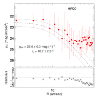
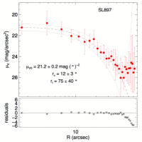
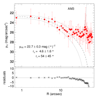
Figure 16: King model fits to SBPs of clusters NGC796, HW20, SL897 and AM3 (from top left to bottom right). Details as in Fig. 14.

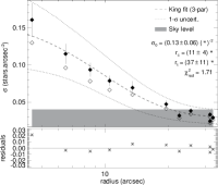
Figure 17: King model fits to RDPs of clusters NGC796, HW20, SL897 and AM3 (from top left to bottom right). Details as in Fig. 15.

Appendix B Isochrone fits charts

This appendix compiles figures resulting from the isochrone fits of the studied clusters, using a MCMC approach, as described in Sect. 5.2. Figs. 18 and 19 shows the posterior distribution of the MCMC parameters used to infer the best model isochrones, and their representations over the clusters CMD.

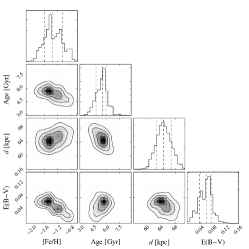
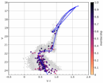
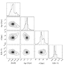
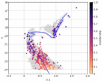
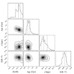
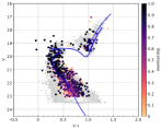
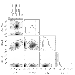
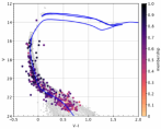
Figure 18: Left: corner plots showing the posterior distribution of the astrophysical parameters derived from MCMC simulations. Right: decontaminated CMDs showing the best model isochrones (solid lines) and the synthetic populations used in the MCMC procedure (gray dots). From top to bottom: AM3, HW20, SL897, NGC796.

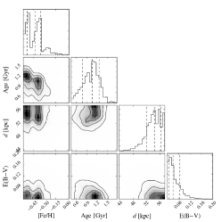
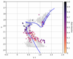
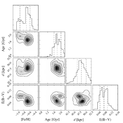
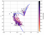
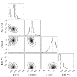
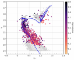
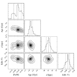
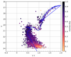
Figure 19: Same as Fig. 18, but for clusters (from top to bottom): KMHK228, OHSC3, SL576, SL61

Appendix C Mass function fitting charts

This appendix compiles the figures resulting from the stellar luminosity and mass function derivations of the studied clusters, as described in Sect. 5.3. Figs. 20 and 21 show the LFs and the power law fits (Eq. 11) over the resulting cluster MFs for the present sample. Total masses and MF slopes are indicated.

Figure 20: Observed and completeness corrected LFs (filled and open histograms, respectively) and MFs (open and filled symbols, respectively). From top left to bottom right: LFs (top panels) and MFs (bottom panels) of AM3, HW20, SL897 and NGC796. The vertical dashed lines correspond to the turn-offs and the solid lines represent the MF fits.

Figure 21: Observed and completeness corrected LFs (filled and open histograms, respectively) and MFs (open and filled symbols, respectively) of LMC clusters. From top left to bottom right: LFs (top panels) and MFs (bottom panels) of KMHK228, OHSC3, SL576 and SL61. The vertical dashed lines correspond to the turn-offs and the solid lines represent the MF fits.

Appendix D List of clusters observed by the VISCACHA survey.

This appendix lists all the clusters observed by the VISCACHA survey up to the 2017B observing run. Their names, equatorial coordinates, observing dates and location in the Magellanic System, respectively, are shown in the columns of Table LABEL:tab:clulist.

Table 6: List of observed clusters

Name	RA (J2000)	Dec (J2000)	Date	Loc.
	[h:m:s]	[ ∘ : ′ : ″ ]	[yyyy-mm-dd]
SL882	06:19:03.2	-72:23:09.0	2015-02-12	LMC
LW458	06:19:10.8	-67:29:37.0	2015-02-12	LMC
LW463	06:19:45.8	-71:18:47.0	2015-02-13	LMC
LW460	06:19:14.7	-71:43:36.0	2015-02-13	LMC
LW459	06:19:16.8	-68:19:39.0	2015-02-13	LMC
LW462	06:19:39.7	-72:16:02.0	2015-02-13	LMC
KMHK1732	06:19:46.4	-69:47:28.0	2015-02-14	LMC
NGC2241	06:22:52.4	-68:55:30.0	2015-02-14	LMC
SL883	06:19:54.6	-68:15:09.0	2015-02-14	LMC
LW469	06:21:33.8	-72:47:24.0	2015-02-23	LMC
OHSC36	06:29:40.6	-70:35:24.0	2015-02-23	LMC
SL889	06:23:28.4	-68:59:50.0	2015-02-23	LMC
SL897	06:33:00.8	-71:07:40.0	2015-02-24	LMC
SL891	06:24:48.6	-71:39:32.0	2015-02-24	LMC
SL892	06:25:14.3	-71:06:08.0	2015-02-24	LMC
SL28	04:44:39.9	-74:15:36.0	2015-12-06	LMC
SL13	04:39:41.7	-74:01:00.0	2015-12-06	LMC
LW15	04:38:25.4	-74:27:48.0	2015-12-06	LMC
SL788	05:55:45.9	-71:11:30.0	2015-12-07	LMC
SL29	04:45:12.3	-75:07:00.0	2015-12-07	LMC
LW62	04:46:17.4	-74:09:36.0	2015-12-07	LMC
SL36	04:46:08.3	-74:53:18.0	2015-12-07	LMC
KMHK1739	06:21:02.5	-71:02:01.0	2016-01-10	LMC
SL53	04:49:53.4	-75:37:42.0	2016-01-10	LMC
SL61	04:50:44.3	-75:32:00.0	2016-01-10	LMC
OHSC1	04:52:40.5	-75:16:36.0	2016-01-11	LMC
SL80	04:52:21.9	-74:53:24.0	2016-01-11	LMC
SL74	04:52:00.4	-74:50:42.0	2016-01-11	LMC
SL886	06:21:24.3	-69:17:56.0	2016-01-11	LMC
OHSC2	04:53:09.7	-74:40:54.0	2016-01-12	LMC
KMHK228	04:53:02.8	-74:00:14.0	2016-01-12	LMC
LW470	06:22:23.3	-72:14:14.0	2016-01-12	LMC
SL84	04:52:44.4	-75:04:30.0	2016-01-12	LMC
LW472	06:23:10.8	-68:19:08.0	2016-01-13	LMC
LW475	06:23:22.9	-70:33:14.0	2016-01-13	LMC
SL118	04:55:31.6	-74:40:36.1	2016-01-13	LMC
SL890	06:23:02.7	-71:41:11.0	2016-01-13	LMC
HW33	00:57:23.0	-70:48:36.0	2016-09-24	SMC
BS95-198	01:48:00.0	-73:07:59.9	2016-09-24	SMC
HW56	01:07:41.2	-70:56:03.6	2016-09-24	SMC
L100	01:18:16.0	-72:00:06.1	2016-09-25	SMC
L73	01:04:23.7	-70:21:12.0	2016-09-25	SMC
NGC422	01:09:35.7	-71:46:23.0	2016-09-25	SMC
HW85	01:42:27.3	-71:16:48.0	2016-09-25	SMC
L32	00:47:23.3	-68:55:32.0	2016-09-25	SMC
HW38	00:59:25.4	-73:49:01.2	2016-09-27	SMC
B94	00:58:16.6	-74:36:28.0	2016-09-27	SMC
HW20	00:44:48.0	-74:21:47.0	2016-09-27	SMC
HW44	01:01:22.0	-73:47:12.1	2016-09-27	SMC
B168	01:26:43.0	-70:46:48.0	2016-09-27	SMC
IC1641	01:09:36.7	-71:46:02.8	2016-09-27	SMC
L114	01:50:19.0	-74:21:24.1	2016-09-28	SMC
K57	01:08:13.8	-73:15:27.0	2016-09-28	SMC
K7	00:27:45.2	-72:46:52.5	2016-09-28	SMC
K55	01:07:32.6	-73:07:17.1	2016-09-28	SMC
HW67	01:13:01.8	-70:57:47.1	2016-09-28	SMC
BS95-75	00:54:31.0	-74:11:06.0	2016-11-02	SMC
B1	00:19:21.3	-74:06:24.1	2016-11-02	SMC
K6	00:25:26.6	-74:04:29.7	2016-11-03	SMC
HW71NW	01:15:30.0	-72:22:36.0	2016-11-03	SMC
BS95-187	01:31:01.0	-72:50:48.1	2016-11-03	SMC
SL53	04:49:54.0	-75:37:42.0	2016-11-03	LMC
L116	01:55:33.0	-77:39:18.0	2016-11-04	SMC
KMHK343	04:55:55.0	-75:08:17.0	2016-11-04	LMC
L112	01:36:01.0	-75:27:29.9	2016-11-04	SMC
SL703	05:44:54.0	-74:50:57.0	2016-11-04	LMC
K9	00:30:00.3	-73:22:40.7	2016-11-04	SMC
NGC152	00:32:56.3	-73:06:56.6	2016-11-05	SMC
AM3	23:48:59.0	-72:56:42.0	2016-11-05	SMC
NGC796	01:56:44.0	-74:13:12.0	2016-11-05	SMC
L113	01:49:30.0	-73:43:40.0	2016-11-05	SMC
HW77	01:20:10.0	-72:37:12.0	2016-11-05	SMC
K37	00:57:48.5	-74:19:31.6	2016-11-05	SMC
HW5	00:31:01.3	-72:20:30.0	2016-11-05	SMC
L114	01:50:19.0	-74:21:24.1	2016-11-05	SMC
IC1708	01:24:57.3	-71:10:59.9	2016-11-05	SMC
L106	01:30:38.0	-76:03:18.0	2016-11-05	SMC

Table 7: continued

List of observed clusters Name RA (J2000) Dec (J2000) Date Loc. [h:m:s] [ ^∘ : ′ : ″ ] [yyyy-mm-dd] IC2148 05:39:12.3 -75:33:47.0 2016-11-30 LMC SL126 04:57:20.0 -62:32:06.0 2016-11-30 LMC SL192 05:02:27.0 -74:51:51.0 2016-11-30 LMC SL576 05:33:13.0 -74:22:08.0 2016-11-30 LMC SL828 06:02:13.0 -74:11:24.0 2016-12-01 LMC SL835 06:04:48.0 -75:06:09.0 2016-12-01 LMC H4 05:32:25.0 -64:44:11.0 2016-12-01 LMC SL647 05:39:35.0 -75:12:30.0 2016-12-02 LMC SL737 05:48:44.0 -75:44:00.0 2016-12-02 LMC LW141 05:07:34.0 -74:38:06.0 2016-12-02 LMC IC2161 05:57:25.0 -75:08:23.0 2016-12-02 LMC LW75 04:50:18.7 -73:38:55.0 2016-12-02 LMC OHSC4 04:59:13.3 -75:07:58.0 2016-12-03 LMC SL783 05:54:39.0 -74:36:19.0 2016-12-03 LMC OHSC3 04:56:36.0 -75:14:29.0 2016-12-03 LMC NGC1755 04:56:55.3 -70:25:28.0 2016-12-03 LMC SL295 05:10:09.0 -75:32:36.0 2016-12-03 LMC Kron11 00:36:27.0 -72:28:44.0 2017-10-20 SMC Kron16 00:40:33.0 -72:44:23.0 2017-10-20 SMC Kron8 00:28:02.0 -73:18:14.0 2017-10-20 SMC NGC362A 01:03:00.0 -70:51:45.0 2017-10-20 SMC Kron47 00:57:47.0 -74:19:36.0 2017-10-20 SMC Lindsay108 01:31:32.0 -71:57:12.0 2017-10-20 SMC Kron15 00:40:13.0 -72:41:55.0 2017-10-20 SMC BS95-196 01:48:02.0 -70:00:12.0 2017-10-20 SMC NGC643 01:35:01.0 -75:33:26.0 2017-10-20 SMC ESO51SC9 00:58:58.0 -68:54:54.0 2017-10-22 SMC HW86 01:42:22.0 -74:10:24.0 2017-10-22 SMC HW66 01:12:04.0 -75:11:54.0 2017-10-22 SMC Kron13 00:35:42.0 -73:35:51.0 2017-10-22 SMC Lindsay32 00:47:24.0 -68:55:12.0 2017-10-22 SMC Lindsay93 01:12:47.0 -73:27:58.0 2017-10-22 SMC NGC121 00:26:49.0 -71:31:58.0 2017-10-22 SMC Lindsay109 01:33:14.0 -74:10:00.0 2017-10-22 SMC KMHK19 04:37:06.0 -72:01:11.0 2017-12-18 LMC KMHK6 04:32:48.0 -71:27:30.0 2017-12-18 LMC KMHK44 04:43:26.0 -64:53:05.0 2017-12-18 LMC ESO85SC03 04:46:56.0 -64:50:25.0 2017-12-19 LMC SL2 04:24:09.7 -72:34:13.0 2017-12-20 LMC BSDL1 04:39:35.7 -70:44:47.0 2017-12-20 LMC DES001SC04 05:24:30.7 -64:19:31.0 2017-12-20 LMC KMHK9 04:34:55.7 -68:14:39.0 2017-12-20 LMC KMHK1593 06:01:49.0 -64:07:58.1 2017-12-20 LMC LW7 04:35:36.7 -69:21:46.0 2017-12-20 LMC NGC1629 04:29:36.7 -71:50:18.0 2017-12-21 LMC KMHK15 04:36:20.7 -70:10:22.0 2017-12-21 LMC KMHK3 04:29:34.0 -68:21:22.0 2017-12-21 LMC HS13 04:35:28.0 -67:42:39.0 2017-12-21 LMC LW20 04:39:57.3 -71:37:07.0 2017-12-21 LMC

References

- Abbott et al. (2018) Abbott T. M. C., et al., 2018, The Astrophysical Journal Supplement Series, 239, 18
- Ahumada et al. (2002) Ahumada A. V., Clariá J. J., Bica E., Dutra C. M., 2002, A&A, 393, 855
- Bastian et al. (2008) Bastian N., Gieles M., Goodwin S. P., Trancho G., Smith L. J., Konstantopoulos I., Efremov Y., 2008, MNRAS, 389, 223
- Baumgardt et al. (2013) Baumgardt H., Parmentier G., Anders P., Grebel E. K., 2013, MNRAS, 430, 676
- Besla (2011) Besla G., 2011, PhD thesis, Harvard University
- Besla et al. (2007) Besla G., Kallivayalil N., Hernquist L., Robertson B., Cox T. J., van der Marel R. P., Alcock C., 2007, ApJ, 668, 949
- Bica & Schmitt (1995) Bica E. L. D., Schmitt H. R., 1995, ApJS, 101, 41
- Bica et al. (1986) Bica E., Dottori H., Pastoriza M., 1986, A&A, 156, 261
- Bica et al. (1996) Bica E., Claria J. J., Dottori H., Santos Jr. J. F. C., Piatti A. E., 1996, ApJS, 102, 57
- Bica et al. (1998) Bica E., Geisler D., Dottori H., Clariá J. J., Piatti A. E., Santos Jr. J. F. C., 1998, AJ, 116, 723
- Bica et al. (2008) Bica E., Bonatto C., Dutra C. M., Santos J. F. C., 2008, MNRAS, 389, 678
- Bica et al. (2015) Bica E., Santiago B., Bonatto C., Garcia-Dias R., Kerber L., Dias B., Barbuy B., Balbinot E., 2015, MNRAS, 453, 3190
- Bressan et al. (2012) Bressan A., Marigo P., Girardi L., Salasnich B., Dal Cero C., Rubele S., Nanni A., 2012, MNRAS, 427, 127
- Burstein & Heiles (1982) Burstein D., Heiles C., 1982, AJ, 87, 1165
- Casetti-Dinescu et al. (2014) Casetti-Dinescu D. I., Moni Bidin C., Girard T. M., Méndez R. A., Vieira K., Korchagin V. I., van Altena W. F., 2014, ApJ, 784, L37
- Chiosi et al. (2006) Chiosi E., Vallenari A., Held E. V., Rizzi L., Moretti A., 2006, A&A, 452, 179
- Choi et al. (2018a) Choi Y., et al., 2018a, ApJ, 866, 90
- Choi et al. (2018b) Choi Y., et al., 2018b, ApJ, 869, 125
- Cioni et al. (2011) Cioni M.-R. L., Clementini G., Girardi L., Guandalini R., Gullieuszik M., et al. 2011, A&A, 527, A116
- Da Costa (1999) Da Costa G. S., 1999, in Chu Y.-H., Suntzeff N., Hesser J., Bohlender D., eds, IAU Symposium Vol. 190, New Views of the Magellanic Clouds. p. 446
- Dias et al. (2014) Dias B., Kerber L. O., Barbuy B., Santiago B., Ortolani S., Balbinot E., 2014, A&A, 561, A106
- Dias et al. (2016) Dias B., Kerber L., Barbuy B., Bica E., Ortolani S., 2016, A&A, 591, A11
- Diaz & Bekki (2012) Diaz J. D., Bekki K., 2012, ApJ, 750, 36
- Diolaiti et al. (2000) Diolaiti E., Bendinelli O., Bonaccini D., Close L., Currie D., Parmeggiani G., 2000, A&AS, 147, 335
- Dobbie et al. (2014) Dobbie P. D., Cole A. A., Subramaniam A., Keller S., 2014, MNRAS, 442, 1680
- Dutra et al. (2001) Dutra C. M., Bica E., Clariá J. J., Piatti A. E., Ahumada A. V., 2001, A&A, 371, 895
- Elson et al. (1987) Elson R. A. W., Fall S. M., Freeman K. C., 1987, ApJ, 323, 54
- Fraga et al. (2013) Fraga L., Kunder A., Tokovinin A., 2013, AJ, 145, 165
- Gaia Collaboration et al. (2016a) Gaia Collaboration et al., 2016a, A&A, 595, A1
- Gaia Collaboration et al. (2016b) Gaia Collaboration et al., 2016b, A&A, 595, A2
- Gaia Collaboration et al. (2018) Gaia Collaboration et al., 2018, A&A, 616, A1
- Gascoigne (1966) Gascoigne S. C. B., 1966, MNRAS, 134, 59
- Geisler et al. (1997) Geisler D., Bica E., Dottori H., Claria J. J., Piatti A. E., Santos Jr. J. F. C., 1997, AJ, 114, 1920
- Girardi et al. (1995) Girardi L., Chiosi C., Bertelli G., Bressan A., 1995, A&A, 298, 87
- Glatt et al. (2008) Glatt K., et al., 2008, AJ, 136, 1703
- Glatt et al. (2010) Glatt K., Grebel E. K., Koch A., 2010, A&A, 517, A50
- Glatt et al. (2011) Glatt K., et al., 2011, AJ, 142, 36
- Gordon & Kron (1983) Gordon K. C., Kron G. E., 1983, PASP, 95, 461
- Grocholski et al. (2006) Grocholski A. J., Cole A. A., Sarajedini A., Geisler D., Smith V. V., 2006, AJ, 132, 1630
- Grocholski et al. (2007) Grocholski A. J., Sarajedini A., Olsen K. A. G., Tiede G. P., Mancone C. L., 2007, AJ, 134, 680
- Harris & Zaritsky (2009) Harris J., Zaritsky D., 2009, AJ, 138, 1243
- Helmi et al. (2018) Helmi A., et al., 2018, A&A, 616, A12
- Hill & Zaritsky (2006) Hill A., Zaritsky D., 2006, AJ, 131, 414
- Hodge (1986) Hodge P., 1986, PASP, 98, 1113
- Jacyszyn-Dobrzeniecka et al. (2016) Jacyszyn-Dobrzeniecka A. M., et al., 2016, Acta Astron., 66, 149
- Kalari et al. (2018) Kalari V. M., Carraro G., Evans C. J., Rubio M., 2018, ApJ, 857, 132
- Kallivayalil et al. (2013) Kallivayalil N., van der Marel R. P., Besla G., Anderson J., Alcock C., 2013, ApJ, 764, 161
- Kennicutt et al. (1996) Kennicutt Jr. R. C., Schweizer F., Barnes J. E., 1996, Galaxies: Interactions and Induced Star Formation
- King (1962) King I., 1962, AJ, 67, 471
- King (1966) King I. R., 1966, AJ, 71, 64
- Kontizas et al. (1985) Kontizas E., Dialetis D., Prokakis T., Kontizas M., 1985, A&A, 146, 293
- Kontizas et al. (1986) Kontizas M., Theodossiou E., Kontizas E., 1986, A&AS, 65, 207
- Kroupa et al. (2013) Kroupa P., Weidner C., Pflamm-Altenburg J., Thies I., Dabringhausen J., Marks M., Maschberger T., 2013, The Stellar and Sub-Stellar Initial Mass Function of Simple and Composite Populations. p. 115, doi:10.1007/978-94-007-5612-0_4
- Lada & Lada (2003) Lada C. J., Lada E. A., 2003, ARA&A, 41, 57
- Landolt (2007) Landolt A. U., 2007, in Sterken C., ed., Astronomical Society of the Pacific Conference Series Vol. 364, The Future of Photometric, Spectrophotometric and Polarimetric Standardization. p. 27
- Lefebvre et al. (2000) Lefebvre M., Keeler R. K., Sobie R., White J., 2000, Nuclear Instruments and Methods in Physics Research A, 451, 520
- Lynga & Westerlund (1963) Lynga G., Westerlund B. E., 1963, MNRAS, 127, 31
- Madore & Arp (1979) Madore B. F., Arp H. C., 1979, ApJ, 227, L103
- Maia et al. (2010) Maia F. F. S., Corradi W. J. B., Santos Jr. J. F. C., 2010, MNRAS, 407, 1875
- Maia et al. (2014) Maia F. F. S., Piatti A. E., Santos J. F. C., 2014, MNRAS, 437, 2005
- Maia et al. (2016) Maia F. F. S., Moraux E., Joncour I., 2016, MNRAS, 458, 3027
- Mastropietro et al. (2005) Mastropietro C., Moore B., Mayer L., Wadsley J., Stadel J., 2005, MNRAS, 363, 509
- Mateo (1988) Mateo M., 1988, ApJ, 331, 261
- Mateo & Hodge (1987) Mateo M., Hodge P., 1987, ApJ, 320, 626
- McLaughlin & van der Marel (2005) McLaughlin D. E., van der Marel R. P., 2005, ApJS, 161, 304
- Miholics et al. (2014) Miholics M., Webb J. J., Sills A., 2014, MNRAS, 445, 2872
- Nayak et al. (2016) Nayak P. K., Subramaniam A., Choudhury S., Indu G., Sagar R., 2016, MNRAS, 463, 1446
- Nidever et al. (2017) Nidever D. L., et al., 2017, AJ, 154, 199
- Nidever et al. (2018) Nidever D. L., et al., 2018, arXiv e-prints, p. arXiv:1805.02671
- Niederhofer et al. (2018) Niederhofer F., et al., 2018, A&A, 613, L8
- Nishiyama et al. (2007) Nishiyama S., et al., 2007, ApJ, 658, 358
- Olsen et al. (2011) Olsen K. A. G., Zaritsky D., Blum R. D., Boyer M. L., Gordon K. D., 2011, ApJ, 737, 29
- Olson & Kwan (1990) Olson K. M., Kwan J., 1990, ApJ, 361, 426
- Olszewski et al. (1991) Olszewski E. W., Schommer R. A., Suntzeff N. B., Harris H. C., 1991, AJ, 101, 515
- Palma et al. (2016) Palma T., Gramajo L. V., Clariá J. J., Lares M., Geisler D., Ahumada A. V., 2016, A&A, 586, A41
- Parisi et al. (2009) Parisi M. C., Grocholski A. J., Geisler D., Sarajedini A., Clariá J. J., 2009, AJ, 138, 517
- Parisi et al. (2014) Parisi M. C., et al., 2014, AJ, 147, 71
- Parisi et al. (2015) Parisi M. C., Geisler D., Clariá J. J., Villanova S., Marcionni N., Sarajedini A., Grocholski A. J., 2015, AJ, 149, 154
- Perren et al. (2017) Perren G. I., Piatti A. E., Vázquez R. A., 2017, A&A, 602, A89
- Piatti (2011) Piatti A. E., 2011, MNRAS, 418, L69
- Piatti & Bastian (2016) Piatti A. E., Bastian N., 2016, A&A, 590, A50
- Piatti & Mackey (2018) Piatti A. E., Mackey A. D., 2018, MNRAS, 478, 2164
- Piatti & Perren (2015) Piatti A. E., Perren G. I., 2015, MNRAS, 450, 3771
- Piatti et al. (2007) Piatti A. E., Sarajedini A., Geisler D., Gallart C., Wischnjewsky M., 2007, MNRAS, 382, 1203
- Piatti et al. (2015) Piatti A. E., de Grijs R., Rubele S., Cioni M.-R. L., Ripepi V., Kerber L., 2015, MNRAS, 450, 552
- Pieres et al. (2016) Pieres A., et al., 2016, MNRAS, 461, 519
- Pieres et al. (2017) Pieres A., et al., 2017, MNRAS, 468, 1349
- Pietrzynski & Udalski (2000) Pietrzynski G., Udalski A., 2000, Acta Astron., 50, 337
- Plummer (1911) Plummer H. C., 1911, MNRAS, 71, 460
- Putman et al. (1998) Putman M. E., et al., 1998, Nature, 394, 752
- Rafelski & Zaritsky (2005) Rafelski M., Zaritsky D., 2005, AJ, 129, 2701
- Ripepi et al. (2014) Ripepi V., et al., 2014, MNRAS, 442, 1897
- Rubele et al. (2018) Rubele S., et al., 2018, MNRAS, 478, 5017
- Santos et al. (1995) Santos Jr. J. F. C., Bica E., Claria J. J., Piatti A. E., Girardi L. A., Dottori H., 1995, MNRAS, 276, 1155
- Santos et al. (2006) Santos Jr. J. F. C., Clariá J. J., Ahumada A. V., Bica E., Piatti A. E., Parisi M. C., 2006, A&A, 448, 1023
- Schlegel et al. (1998) Schlegel D. J., Finkbeiner D. P., Davis M., 1998, ApJ, 500, 525
- Searle et al. (1980) Searle L., Wilkinson A., Bagnuolo W. G., 1980, ApJ, 239, 803
- Sitek et al. (2017) Sitek M., et al., 2017, Acta Astron., 67, 363
- Skowron et al. (2014) Skowron D. M., et al., 2014, ApJ, 795, 108
- Stetson (1987) Stetson P. B., 1987, PASP, 99, 191
- Stetson (2000) Stetson P. B., 2000, PASP, 112, 925
- Subramanian et al. (2017) Subramanian S., et al., 2017, MNRAS, 467, 2980
- Udalski et al. (2015) Udalski A., Szymański M. K., Szymański G., 2015, Acta Astron., 65, 1
- Werchan & Zaritsky (2011) Werchan F., Zaritsky D., 2011, AJ, 142, 48
- Wilson (1975) Wilson C. P., 1975, AJ, 80, 175
- Wolf et al. (2018) Wolf C., et al., 2018, Publ. Astron. Soc. Australia, 35, e010
- Zaritsky et al. (1996) Zaritsky D., Schectman S. A., Bredthauer G., 1996, PASP, 108, 104
- Zaritsky et al. (1997) Zaritsky D., Harris J., Thompson I., 1997, AJ, 114, 1002
- Zaritsky et al. (2002) Zaritsky D., Harris J., Thompson I. B., Grebel E. K., Massey P., 2002, AJ, 123, 855
- Zaritsky et al. (2004) Zaritsky D., Harris J., Thompson I. B., Grebel E. K., 2004, AJ, 128, 1606
- Zivick et al. (2018) Zivick P., et al., 2018, ApJ, 864, 55
- van der Marel & Kallivayalil (2014) van der Marel R. P., Kallivayalil N., 2014, ApJ, 781, 121
- van der Marel & Sahlmann (2016) van der Marel R. P., Sahlmann J., 2016, ApJ, 832, L23
- van der Marel et al. (2009) van der Marel R. P., Kallivayalil N., Besla G., 2009, in Van Loon J. T., Oliveira J. M., eds, IAU Symposium Vol. 256, The Magellanic System: Stars, Gas, and Galaxies. pp 81–92 (arXiv:0809.4268), doi:10.1017/S1743921308028299