Combining Physically-Based Modeling and Deep Learning for Fusing GRACE Satellite Data: Can We Learn from Mismatch?
Abstract
Global hydrological and land surface models are increasingly used for tracking terrestrial total water storage (TWS) dynamics, but the utility of existing models is hampered by conceptual and/or data uncertainties related to various underrepresented and unrepresented processes, such as groundwater storage. The gravity recovery and climate experiment (GRACE) satellite mission provided a valuable independent data source for tracking TWS at regional and continental scales. Strong interests exist in fusing GRACE data into global hydrological models to improve their predictive performance. Here we develop and apply deep convolutional neural network (CNN) models to learn the spatiotemporal patterns of mismatch between TWS anomalies (TWSA) derived from GRACE and those simulated by NOAH, a widely used land surface model. Once trained, our CNN models can be used to correct the NOAH simulated TWSA without requiring GRACE data, potentially filling the data gap between GRACE and its follow-on mission, GRACE-FO. Our methodology is demonstrated over India, which has experienced significant groundwater depletion in recent decades that is nevertheless not being captured by the NOAH model. Results show that the CNN models significantly improve the match with GRACE TWSA, achieving a country-average correlation coefficient of 0.94 and Nash-Sutcliff efficient of 0.87, or 14% and 52% improvement respectively over the original NOAH TWSA. At the local scale, the learned mismatch pattern correlates well with the observed in situ groundwater storage anomaly data for most parts of India, suggesting that deep learning models effectively compensate for the missing groundwater component in NOAH for this study region.
WRR
Bureau of Economic Geology, Jackson School of Geosciences, The University of Texas at Austin, Austin, TX, USA
State Key Laboratory of Geodesy and Earth’s Dynamics, Institute of Geodesy and Geophysics, Chinese Academy of Sciences, Wuhan 430077, China Texas Advanced Computing Center, The University of Texas at Austin, Austin, TX, USA Department of Geology and Geophysics, Indian Institute of Technology Kharagpur, West Bengal 721302, India
A. Y. Sunalex.sun@beg.utexas.edu
1 Introduction
Terrestrial total water storage (TWS) is a key element of the global hydrological cycle, affecting both water and energy budgets (Rodell and Famiglietti, 2001). Tracking the TWS on a periodic basis was historically difficult because of the lack of reliable in situ observations (Seneviratne et al., 2004), a situation that is still true in most countries. The gravity recovery and climate experiment (GRACE) satellite mission provided unprecedented tracking of the global TWS dynamics during its 15-year mission (2002-2017). GRACE enabled remote sensing of TWS anomalies (TWSA) (i.e., variations from a long-term mean) at regional to continental scales (> 100,000 km2). The availability of such information has had a profound impact on the development and validation of regional and global hydrological models, which are increasingly being used to assess changes in the hydrological cycle under current and future climate conditions. These physically-based, semi-distributed hydrological models are built on mathematical abstractions of physical processes that govern the movement and storage of water, as well as land surface energy partitioning in certain models, in space and time. Despite its coarse resolution, GRACE provides a “big picture” check of model simulated TWS variations and thus represents a valuable independent source of information for diagnosing and improving the model performance. So far, GRACE data has been used in model calibration and parameter estimation (Werth and Güntner, 2010; Lo et al., 2010; Milzow et al., 2011; Sun et al., 2012) and data assimilation (Houborg et al., 2012; Li et al., 2012; van Dijk et al., 2014; Girotto et al., 2016; Schumacher et al., 2016; Khaki et al., 2017). While results of these studies all indicate that the assimilation of GRACE data generally improves model skills, the improvements may be limited by uncertainties in model parameters and structures (e.g., missing deep groundwater storage and agricultural irrigation), as well as assumptions underlying data assimilation schemes (e.g., a priori specified spatial and temporal error covariance structures) (Girotto et al., 2016). Calibration against an imperfect model structure using inaccurate error models may lead to information loss and greater propensity for forecast error (Gupta and Nearing, 2014). A recent study compared TWSA trends obtained from seven global hydrological models with those derived from GRACE over 186 global river basins (Scanlon et al., 2018). Their results indicate a large spread in model results and poor correlation between models and GRACE, which were attributed by the authors to the lack of surface water and groundwater storage components in most land surface models (LSMs), low storage capacity in all models, uncertainties in climate forcing, and lack of representation of human intervention in most LSMs.
Unlike physically-based models, pure data-driven methods (black box models) seek to establish a regression model between climate forcing (e.g., precipitation and temperature) and GRACE TWS (Long et al., 2014; Humphrey et al., 2017; Seyoum and Milewski, 2017), or between TWS and its various components (Sun, 2013; Zhang et al., 2016; Miro and Famiglietti, 2018). Data-driven models are suitable for applications where there are plenty of observations but a complete understanding of the underlying physical processes is lacking. A common criticism of black box models, however, is related to their lack of interpretability and generalizability—a regression model trained on the premise of a strong correlation between predictors and the predictand may give unreliable results whenever and wherever such correlation is weak. In addition, pure data-driven models often do not integrate the full stack of information (e.g., soil property, topography, and vegetation types) that is normally represented in physically-based models and therefore are only limited to simulating certain aspects (e.g., interannual variations) of a physical process. It is thus desirable to apply knowledge gained from decades of physical-based modeling to inform the development of data-driven models. These hybrid physical science and data science methods will help to bridge and thus benefit hypothesis-driven and data-driven discoveries (Karpatne et al., 2017).
In this work we apply a hybrid approach that combines the strengths of physically-based modeling and deep learning. Specifically, we use deep convolutional neural networks (CNN), which are a special class of artificial neural networks, to learn the spatiotemporal patterns of “mismatch” between the TWSA simulated by an LSM and that observed by GRACE. Here the term mismatch broadly refers to the difference either between two datasets or between model simulations and observations. The learned mismatch patterns are then fed back to the LSM to compensate for deficiencies in the LSM. That means once trained and validated, the CNN model may be used to predict the observed TWSA without requiring GRACE TWSA as inputs, thus potentially filling the data gap between GRACE and its follow-on mission (GRACE-FO). In the same fashion, the trained CNN model may also be used to reconstruct TWSA for the pre-GRACE era. The basic principle underlying our hybrid modeling approach is similar to that behind data assimilation methods, both exploiting mismatch patterns between predicted and observed variables. However, the assimilation part of our hybrid method is driven by deep learning models that set the current state-of-the-art in computer vision, and not limited by the Gaussian-like unimodal error distribution commonly assumed in many data assimilation schemes. On the other hand, the spatiotemporal propagation part of our method is driven by a physically based LSM, mitigating the lack of spatial continuity and physical interpretation in purely data-driven statistical models.
As a case study, we demonstrate our hybrid approach over India, where irrigation-induced groundwater depletion has been confirmed by GRACE and in situ studies (Rodell et al., 2004; Chen et al., 2014; Long et al., 2016; MacDonald et al., 2016), but is not well resolved in many contemporary LSMs. We evaluate the performance of three different types of CNN models, driven under different predictor combinations. Compared to the original LSM, we show that all CNN models considered here significantly improve the performance of the corrected LSM model, both at the country and grid scales. In the following, Section 2 describes the study area and data used, Section 3 provides details on the technical approach, and results and discussions are given in Section 4.
2 Data and Data Processing
2.1 Description of the study area, India
A large part of the annual rainfall budget over the Indian subcontinent can be attributed to the Indian Summer monsoon (ISM), which results from interactions of several complex atmospheric processes evolving over many different spatiotemporal scales and is modulated by the steep topography of the Himalayas (Bookhagen and Burbank, 2010). The entire Indian region (except for the southern part) receives maximum precipitation during the monsoon season, which typically lasts from June to September. At the country level, the average rainfall received during the monsoon season is 85 cm, amounting to about 78% of the annual rainfall (Mooley and Parthasarathy, 1984). In the southern part of the country, the monsoon season extends to October, sometimes even to November (Bhanja et al., 2016).
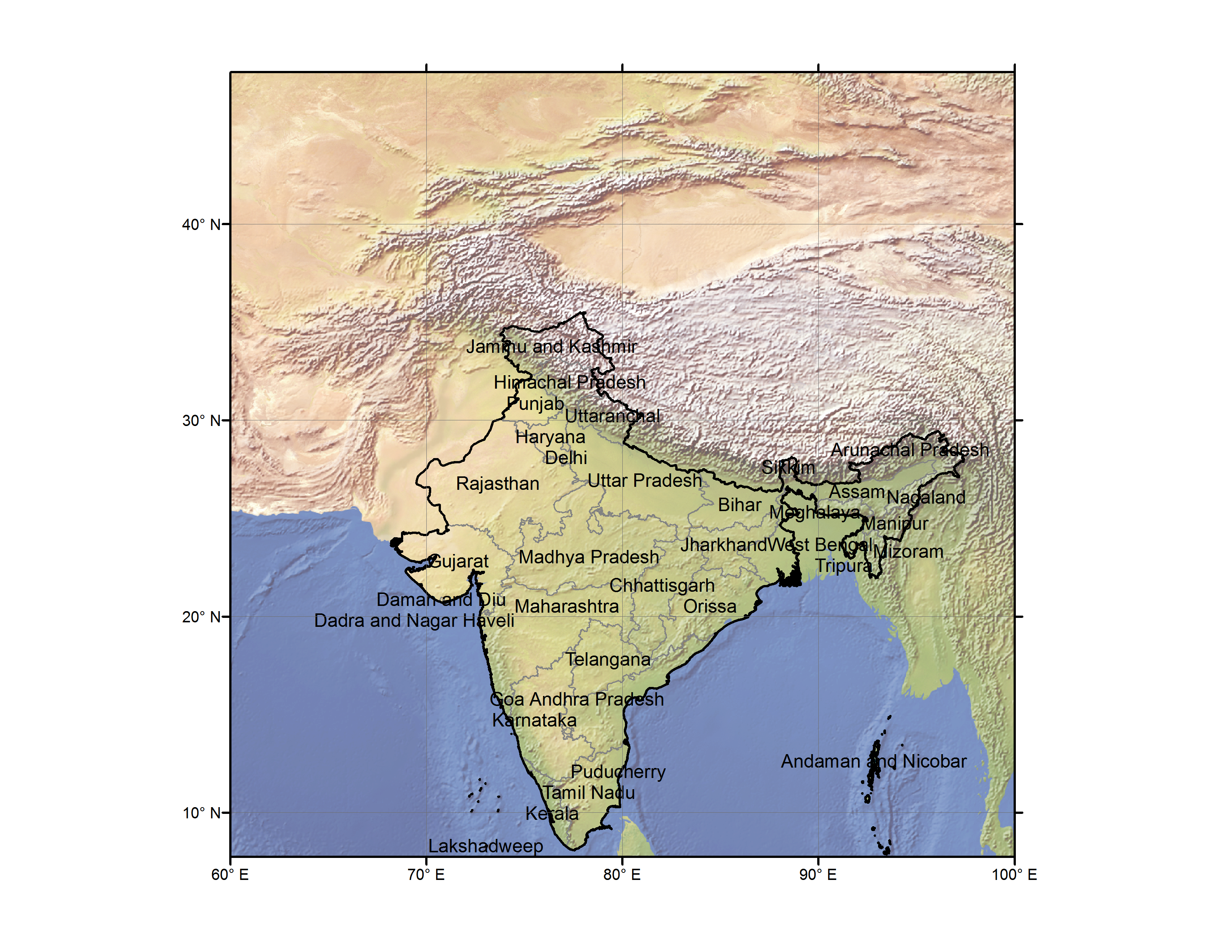
India depends heavily on groundwater resources. Groundwater storage is a function of climatic variables such as precipitation and evaporation, particularly in areas with shallow groundwater tables (Bhanja et al., 2016). The Indus–Ganges–Brahmaputra systems, which together drain the northern Indian plains, form a regional alluvial aquifer system that is regarded as one of the most productive aquifers of the world; on the other hand, groundwater is available in a limited extent within the weathered zone and underlying fractured aquifers within the remaining two-thirds of the country (Mukherjee et al., 2015). Irrigation withdrawal accounts for over 90% of the total groundwater uses (India Central Ground Water Board, 2014). Overuse of groundwater beyond its potential has caused pronounced groundwater depletion in northwest India, including the states of Punjab, Haryana and Delhi, and Rajasthan (Figure 1). The country has established a dense in situ groundwater monitoring network. Groundwater level measurements are taken on a seasonal basis in January, April/May, August, and November, from a network of piezometers (4,939) and non-pumping observation wells (10,714) that are typically screened in the first available aquifer below ground surface (Bhanja et al., 2016).
The extensive in situ groundwater monitoring coverage shall provide additional information for cross-validating patterns learned by the deep CNN models. This study uses the in situ groundwater dataset published recently by Bhanja et al. (2016), which consists of 3,989 wells that were selected to have temporal continuity (i.e., at least 3 out of 4 seasonal data should be available in all years). The authors derived groundwater storage anomalies from water level measurements by using specific yield values corresponding to 12 major river basins in the country. The temporal coverage of the dataset is from January 2005 to November 2014. More details on the data processing and quality control can be found in Bhanja et al. (2016).
Besides groundwater, the impact of surface water is relatively high along Indus River and Ganges River, but is generally small in the area of severe groundwater depletion in northwest India (Getirana et al., 2017).
2.2 GRACE-derived TWSA
This study uses the monthly mascon TWSA product (RL-05) released by Jet Propulsion Laboratory (JPL) (https://grace.jpl.nasa.gov), which has a 0.5°×0.5° grid resolution, but inherently represents 3°×3° equal-area caps (Watkins et al., 2015). The period of study covers from April 2002 to December 2016. Uncertainty in GRACE data is related to both measurement and leakage errors, leading to potential signal loss (Wiese et al., 2016). Measurement errors are related to, for example, system-noise error in the inter-satellite range-rate and accelerometer error (Swenson et al., 2003). Leakage errors arise because boundaries of hydrological basins generally do not conform to the boundaries of the mascon elements and because leakage across land/ocean boundaries (i.e., from mascons that cover both land and ocean). For this work, we applied the gain factor (scaling factor) distributed with the JPL mascon to compensate for the signal loss. The gain factor, when combined with coastal line resolution improvement, was shown to reduce leakage errors associated with mass balance of large river basins (>160,000 km2) by an amount of 0.6–1.5 mm equivalent water height averaged globally (Wiese et al., 2016). We obtained the total uncertainty bound of monthly TWSA for the study region by combining the measurement error released by JPL with the estimated leakage error. The leakage error was estimated using the method of Wiese et al. (2016).
2.3 NOAH land surface model
The NOAH LSM from NASA’s global land data assimilation system (GLDAS) (Rodell et al., 2004) has been extensively used in previous GRACE studies. Like many other LSMs, NOAH maintains surface energy and water balances and simulates the exchange of water and energy fluxes at soil-atmosphere interface (Ek et al., 2003). NOAH does not simulate surface water storage (SWS) (e.g., in rivers, lakes, and wetlands) and surface runoff routing, nor does it account for deep groundwater storage and human intervention. The roles of SWS and GWS can be significant in various parts of the study area, as mentioned previously. For this study, the monthly forcing (total precipitation and average air temperature at 2m) and outputs of NOAH V2.1 (0.25°×0.25°) were downloaded from NASA’s EarthData site (http://earthdata.nasa.gov). The NOAH-simulated TWS was calculated by summing soil moisture in all four soil layers (spanning from 0–200 cm depth), accumulative snow water, and total canopy water storage (the contribution of canopy water is typically negligible but is included for completeness). To be consistent with the GRACE TWSA processing, the long-term mean from January 2004 to December 2009 was subtracted from NOAH TWS to obtain the simulated TWSA.
3 Methodology
3.1 Model and GRACE TWSA mismatch
TWS is the sum of the following components (Scanlon et al., 2018):
| (1) |
where SnWS represents snow water storage, CWS is canopy water storage, SWS is surface water storage, SMS is soil moisture storage, and GWS is groundwater storage. We define the difference or mismatch between NOAH-simulated TWSA and GRACE TWSA at time as
| (2) |
where the mismatch , which varies in both space and time, may be related to two types of errors, (a) systematic error or bias caused by either missing processes or uncertain conceptualization in NOAH (e.g., omission of GWS), and (b) random error related to uncertain data and model parameters. For the purpose of this work, we use CNN models to learn a functional relationship between and its predictors by solving a regression problem
| (3) |
where is a CNN model; denotes the network parameters to be solved by using as training data, where is the index of training samples, is a set of input samples from different predictors , and are samples of obtained by using Eq. 2. After training and validation, the CNN model can be used to predict and, thus, give corrected TWSA without requiring GRACE data.
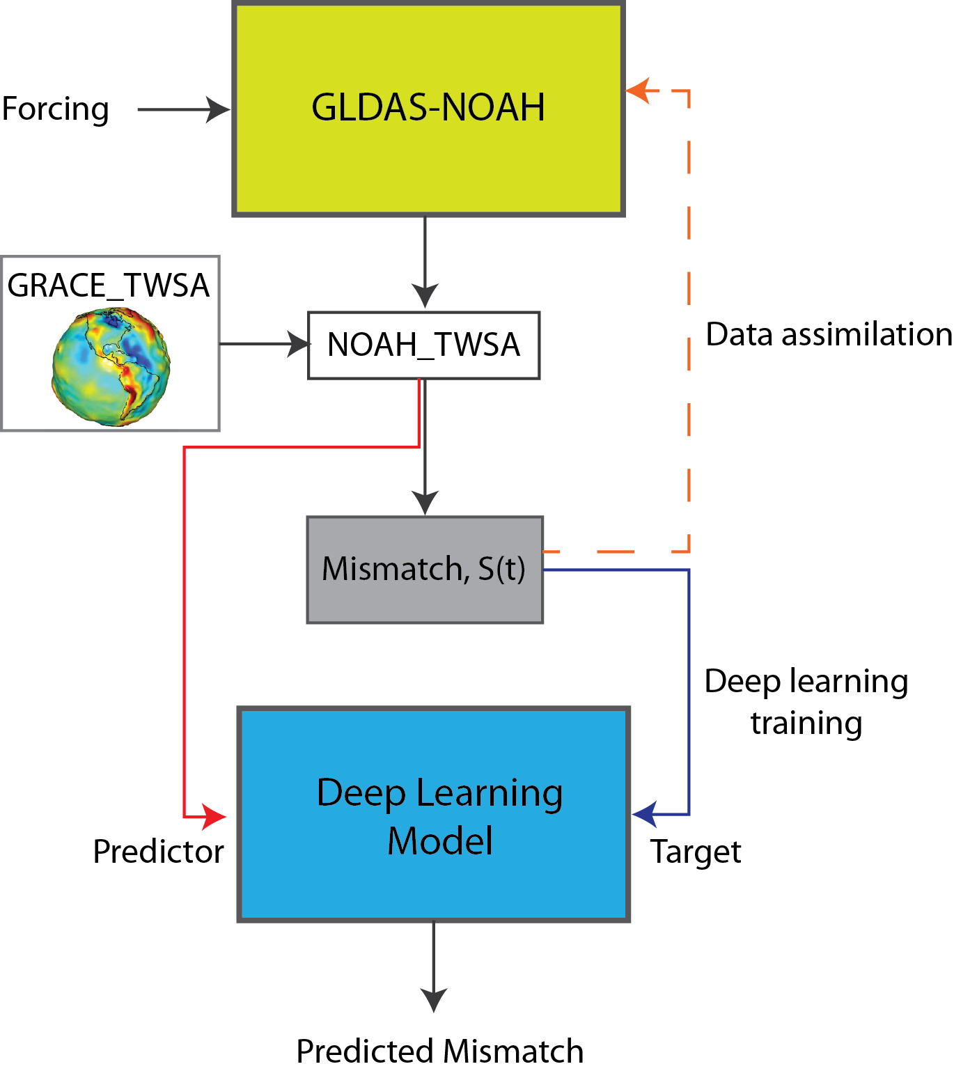
Figure 2 further illustrates the relations among NOAH, GRACE, and the deep learning model, and the proposed workflow. The deep learning workflow (solid line) is similar to that used in the traditional data assimilation (dashed line), both exploiting the residual between model and observations. The main difference is that in deep learning the GRACE TWSA data is not used to correct the model states but to train a regression model for predicting the mismatch, circumventing challenges related to calibrating a conceptually uncertain physical model. Details on the design and architecture of the CNN models are provided in the subsection below.
3.2 Design and architectures of CNN deep learning models
CNN, originally introduced by LeCun (LeCun, 1989; LeCun and Bengio, 1995), is symbolic of the modern deep learning era that began around 2006 (Schmidhuber, 2015). CNNs and their variants have been extensively used in image classification and are behind several high-profile deep learning model architectures that have won the ImageNet Large Scale Visual Recognition Challenge (ILSVRC) in recent years (Simonyan and Zisserman, 2014; LeCun et al., 2015; Szegedy et al., 2015; He et al., 2016). The design of CNN was inspired by the human visual cortex, aiming to extract subtle features embedded in the inputs. As its name suggests, CNN applies discrete convolution operations to project an input image (or a stack of images) onto a hierarchy of feature maps, which may be thought of as nonlinear transformations of the input. In practice, a CNN deep learning model architecture includes the input, output, and a series of hidden convolution layers in between to extract spatial features (e.g., edges and corners) from each layer’s input. Thus, by design CNN models are highly suitable for learning multiscale spatial patterns from multisource gridded data, which is a challenging problem to solve using the traditional multilayer perception neural network models that do not scale well on images.
In a convolution operation, a moving window, commonly referred to as a filter or kernel, is used to scan along each dimension of the input image, with possible strides between the moves (a stride defines the number of rows/columns to skip). For each move, a dot product is taken between the filter parameters and the underlying input image patch, leading to a feature map at the end of scanning. The dimensions (width and height ) of a feature map are related to its input as
| (4) |
where and are dimensions of the input image, and are dimensions of the feature map, is the filter dimension, is the stride size, and is padding size. Filter dimensions and stride sizes are commonly kept the same for both dimensions. Eq. 4 suggests that the dimensions of a feature map become progressively smaller after each convolution operation. Zero-padding may be used to add zeros around the edges of the output feature map (i.e., in Eq. 4) to preserve the input dimensions.
CNN naturally achieves sparsity because each pixel in a feature map only connects to a small region in its input layer. Also, by applying the same filter to scan the entire input image, the filter parameters are shared and the resulting feature map is equivariant to shifts in inputs. Specifically, the units of a convolutional layer , , is related to feature maps of its preceding layer , , by (Goodfellow et al., 2016)
| (5) |
where is the number of feature maps in layer , denotes the convolution operator, are the filter parameters, are the bias parameters, and is the activation function. Eq. (5) shows that CNN involves a hierarchy of feature maps, with each layer learning from its preceding layer. When (i.e., the first hidden layer), its input layer simply becomes the actual input image(s). The Rectified Linear Unit (ReLU) function
| (6) |
is commonly used as the activation function for hidden CNN layers, which is less costly to compute than other nonlinear functions (e.g., sigmoid) and is shown to improve the CNN training speed significantly (Goodfellow et al., 2016). In regression problems, the linear function or hyperbolic tangent function (tanh) are often used as the activation functions for the output layer to generate solution in the real domain. The total number of CNN parameters (weights and biases) is determined by the number of filters, filter dimensions, and stride dimensions, which are considered hyperparameters of the CNN model design and may be tuned during training.
In addition to convolution operation, other commonly used CNN layer operations include pooling, dropout, and batch normalization. Pooling aggregates information in each moving window to further reduce the size of feature maps. For example, max pooling selects the maximum element in a pooling window. Dropout operation randomly leaves out certain number of hidden neurons during training so that the net effect is to prevent the network from overfitting; thus, it is regarded as a regularization technique. Batch normalization performs normalization on hidden layers to improve network training speed and stability (Goodfellow et al., 2016).
Figure 3 shows a high-level, architectural diagram of CNN deep learning models considered in this work. Because the number of training samples (labeled data) is limited for many geoscience problems including the one at hand, we tested several techniques to improve the performance of CNN models, including (a) augmenting the NOAH TWSA training samples with additional predictors, such as precipitation (P) and temperature (T), (b) including regions outside the study area (i.e., spanning 60–100° longitude, 7.75–47.75° latitude, as shown in Figure 1) in training to reduce potential boundary effects and increase training information, and (c) transfer learning, which “borrows” the weights from a CNN model trained using many other images. Precipitation and temperature are already part of the NOAH forcing. The logic behind including them as additional predictors is that not all the information in the forcing is fully utilized by the LSM. For example, precipitation contributes to surface water and groundwater recharge that are not simulated by NOAH. Similarly, temperature is a proxy of evapotranspiration, which may not be simulated accurately by the model. Humphrey et al. (2017) suggested that at least 40% of the total variance of GRACE anomalies can be reconstructed from precipitation and temperature variability alone. Thus, in this study precipitation and temperature are explored as additional predictors to help improve the model prediction.
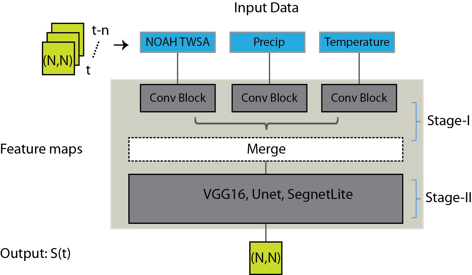
As part of data preparation, all input data are formatted or resampled into 2D images of equal dimensions. Specifically, the 40°×40° square region used in this study is represented by 128×128 pixel images (0.3125° per pixel). The input and target images are normalized before training. Hydroclimatic variables typically exhibit certain temporal correlation. To enable the CNN to explore temporal correlation between each input variable and its antecedent conditions, we stack the input image at time on top of its antecedent conditions to form a 3D volume (see Figure 3). We set the number of lags to 2 (i.e., ) after preliminary experiments; thus each input volume has dimensions 128×128×3. Figure 3 shows that our model design includes two learning stages. In Stage I, each input volume goes through a separate stack of convolutional layers. In Stage II, feature maps resulting from Stage I are merged and the results are fed to a deep learning model to arrive at the final outputs. The first stage aims to extract unique features from each input, while the second stage aims to perform deep learning of the spatial and temporal patterns within each input, as well as co-variation patterns across the inputs. Putting in a different way, the role of Stage I is to prepare inputs for use with the problem-independent, established CNN model architectures employed in Stage II.
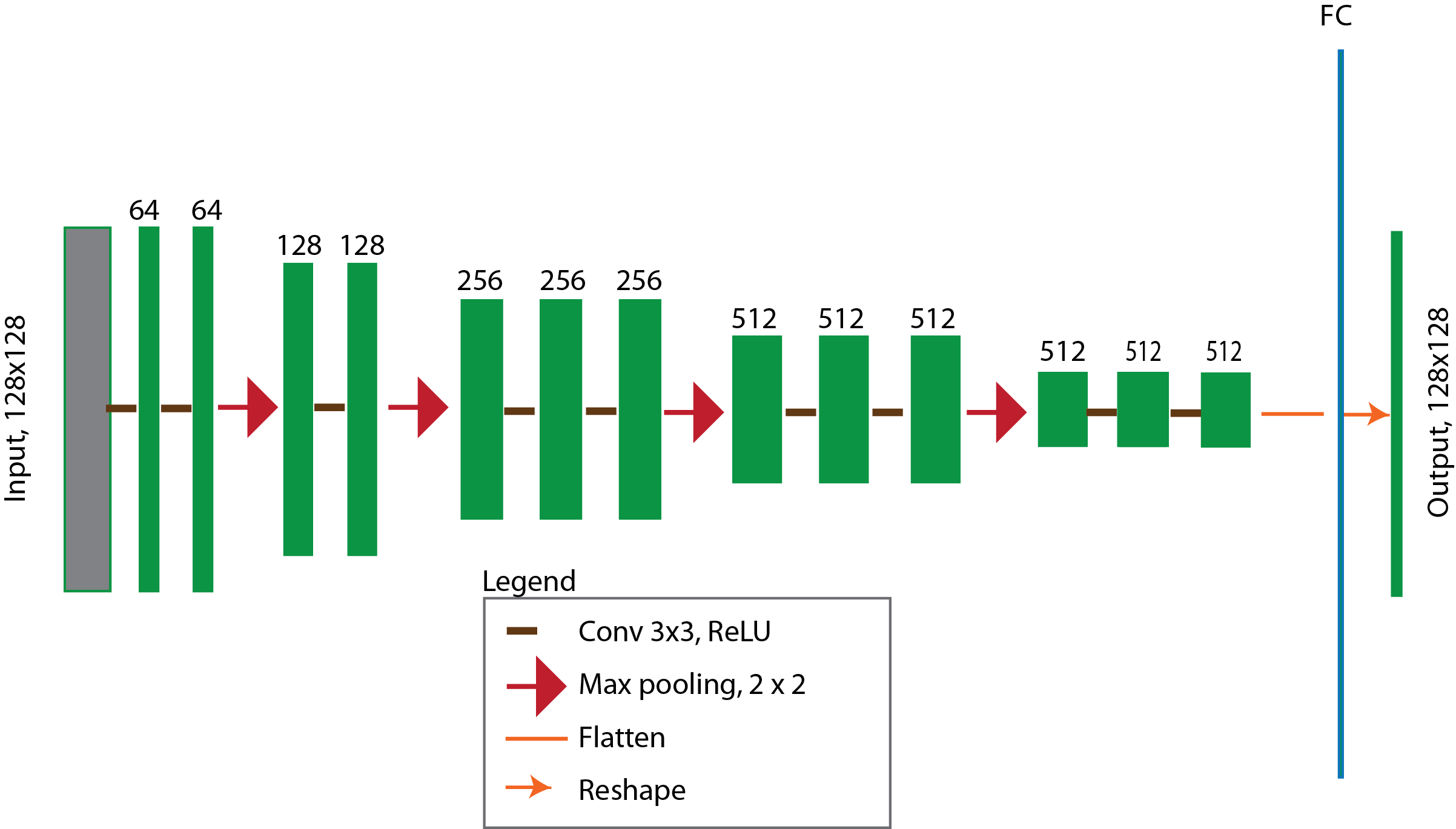
In this work, we consider three CNN-based model architectures, VGG16, Unet, and Segnet, commonly used in image semantic segmentation problems (i.e., associating each pixel of an image with a class label). VGG16 is a CNN-based model architecture consisting of 16 layers of 3×3 convolutional layers, 2×2 max pooling layers, and then a fully connected layer at the end (Appendix A1). The number of filters used in each VGG16 convolutional layers monotonically increases. A VGG16 model pre-trained using 1.3 million images from the ILSVRC-2012 dataset (Simonyan and Zisserman, 2014) is adopted in this work to implement transfer learning. In , this is equivalent to freezing all the hidden layers in VGG16, except for the last fully connected layer, during training. This way, the CNN model will be able to adjust itself to the user-specific inputs while transferring most of the weights learned from the ILSVRC-2012, which includes labeled images of 1000 object classes (Russakovsky et al., 2015). Previously, Jean et al. (2016) used transfer learning models to predict poverty based on satellite imagery. They showed that transfer learning “can be productively employed even when data on key outcomes of interest are scarce.” Questions remain about the general applicability of transfer learning to satellite images, which are very different from the images used in the ILSVRC dataset.
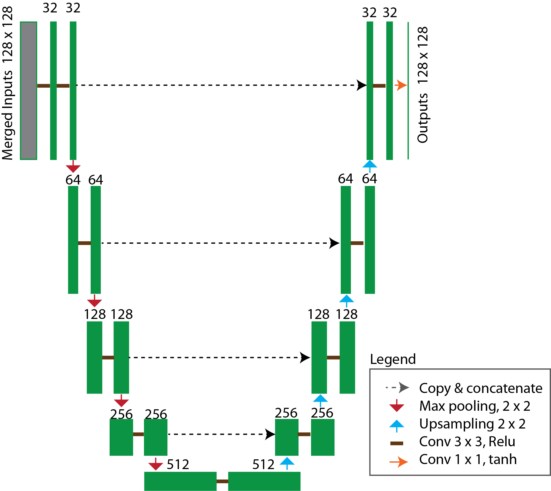
Unet has demonstrated superb performance on semantic segmentation problems, especially on relatively small training datasets (Ronneberger et al., 2015). Unet belongs to a class of encoder-decoder model architectures. It consists of an encoding path (downsampling steps) to capture image context, followed by a symmetric decoding path (upsampling steps) to enable precise localization (Appendix A2). The Unet model architecture used in this study is shown in Appendix A2. It consists of repeated applications of two 3×3 convolution operations, each followed by a 2×2 max pooling layer. The number of filters used is doubled after each downsampling step and then halved after each upsampling step. In the final step, a convolutional layer is used to generate the output. Unet models are characterized by the copy and concatenation operations that combine the higher resolution features from the downsampling path with the upsampled features at the same level to better localize and learn representations (dashed line with arrow in Figure A.2). This is also the part of Unet that enables multiscale learning.
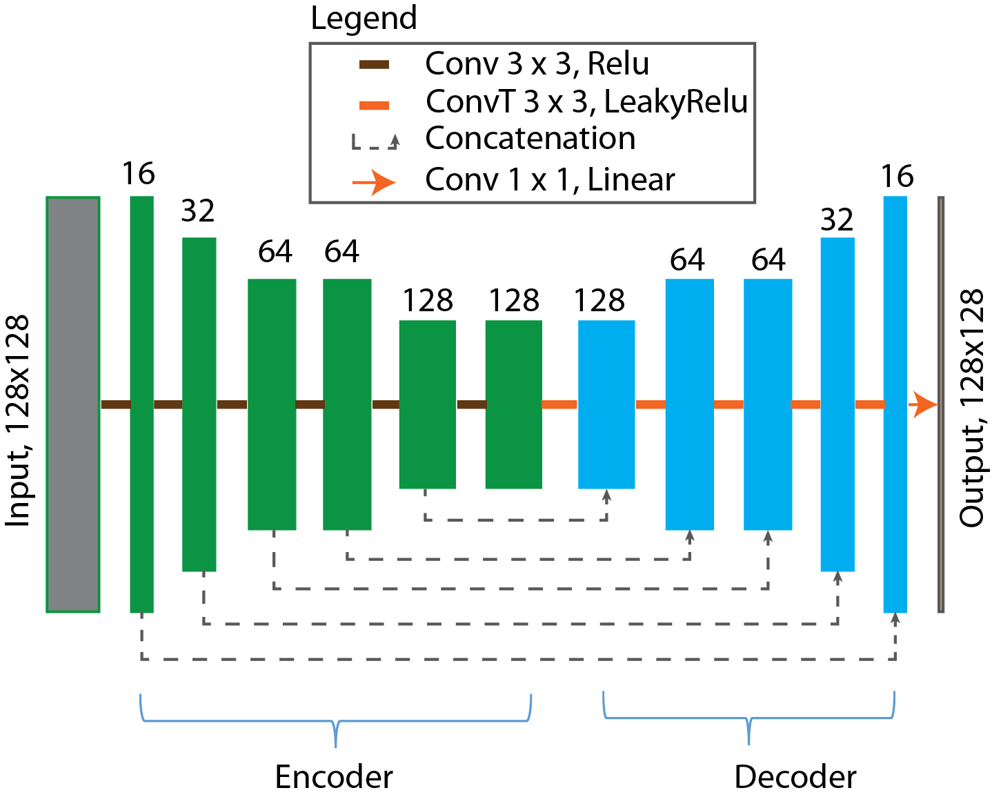
Segnet is also a class of encoder-decoder architecture that was originally introduced to solve image segmentation problems (Badrinarayanan et al., 2015). Similar to the Unet architecture, it includes an encoding path and a decoding path. The main difference between the design of the original Segnet and Unet is that the decoder in Segnet uses pooling indices computed in the max-pooling step of the corresponding encoder to perform non-linear upsampling, while in Unet the concatenation step is done before the pooling step. Thus, the number of parameters of Segnet is smaller than that in the Unet. In this work, we use a variant of the Segnet architecture, in which the pooling layers are removed and the upsampling layers in the decoder are replaced by transpose convolution layers, which may be regarded as performing the reverse of convolutional operations (Zeiler et al., 2010). Different from upsampling, transpose convolution layers have trainable parameters. The model design is shown in Appendix A3, which we shall refer to as the SegnetLite in the rest of this discussion. Similar to Unet, SegnetLite also uses concatenation steps to combine feature maps from encoding and decoding steps. The SegnetLite model has a significantly smaller number of trainable parameters (~700 thousand) than Unet (7.8 million) and VGG16 (~134 million ), and can be trained more efficiently.
For Unet and SegnetLite models, Stage I shallow learning (Figure 3) includes a single convolutional layer with 16 filters for each type of predictors, the outputs of which are then merged and provided as inputs to the respective deep learning model. In the case of VGG16, the maximum number of filters that can be used in Stage I is 3. This is because the trained VGG16 is designed to process images, which only allow 3 color channels (RGB).
3.3 Training and testing of CNN models
The open-source Python package Keras with the Tensorflow backend (Chollet et al., 2015) is used to develop all CNN models presented in this work. Unless otherwise specified, the stochastic gradient descent optimizer is used to train the CNN models with a learning rate of 0.01, decay rate of , and momentum of 0.9. Out of a total of 177 monthly data available for the study period, 125 months or 70% is used for training and the rest for testing. The loss or objective function used for network training is the weighted sum of two fitting criteria
| (7) |
in which and are the predicted and observed mismatch at grid cell and month , denotes temporal average at cell , is the number of grid cells in the study area, is the number of training samples in the training period, and the summation is taken both spatially and temporally. Criterion 1 is the commonly used mean square error (MSE) and Criterion 2 is a modified form of the Nash-Sutcliff efficiency (NSE) that is more sensitive to over- or underprediction than the L2 forms used in NSE (Krause et al., 2005; Sun and Sun, 2015). The weight between two criteria is a hyperparameter and is set to 0.5 in this work.
The performance of trained models is evaluated against the observed GRACE TWSA using correlation coefficient and NSE. For spatially averaged time series, the NSE is defined as
| (8) |
in which (°) denotes spatially-averaged quantities and denotes the temporal mean of observed values, and is the number of samples used for evaluation. The range of NSE is 1].
All experiments are carried out on a Linux machine (Dell PowerEdge R730 server) running with GPU (NVIDIA Tesla K80 GPU, 24Gb RAM total). Training typically takes 4s, 3s, and <1s per epoch for VGG16, Unet, and SegnetLite, respectively. Epoch is a deep learning term that refers to a full pass through a given training dataset and each epoch may include several iterations as determined by the batch size (i.e., the number of samples passed to the neural network during each training iteration).
4 Results
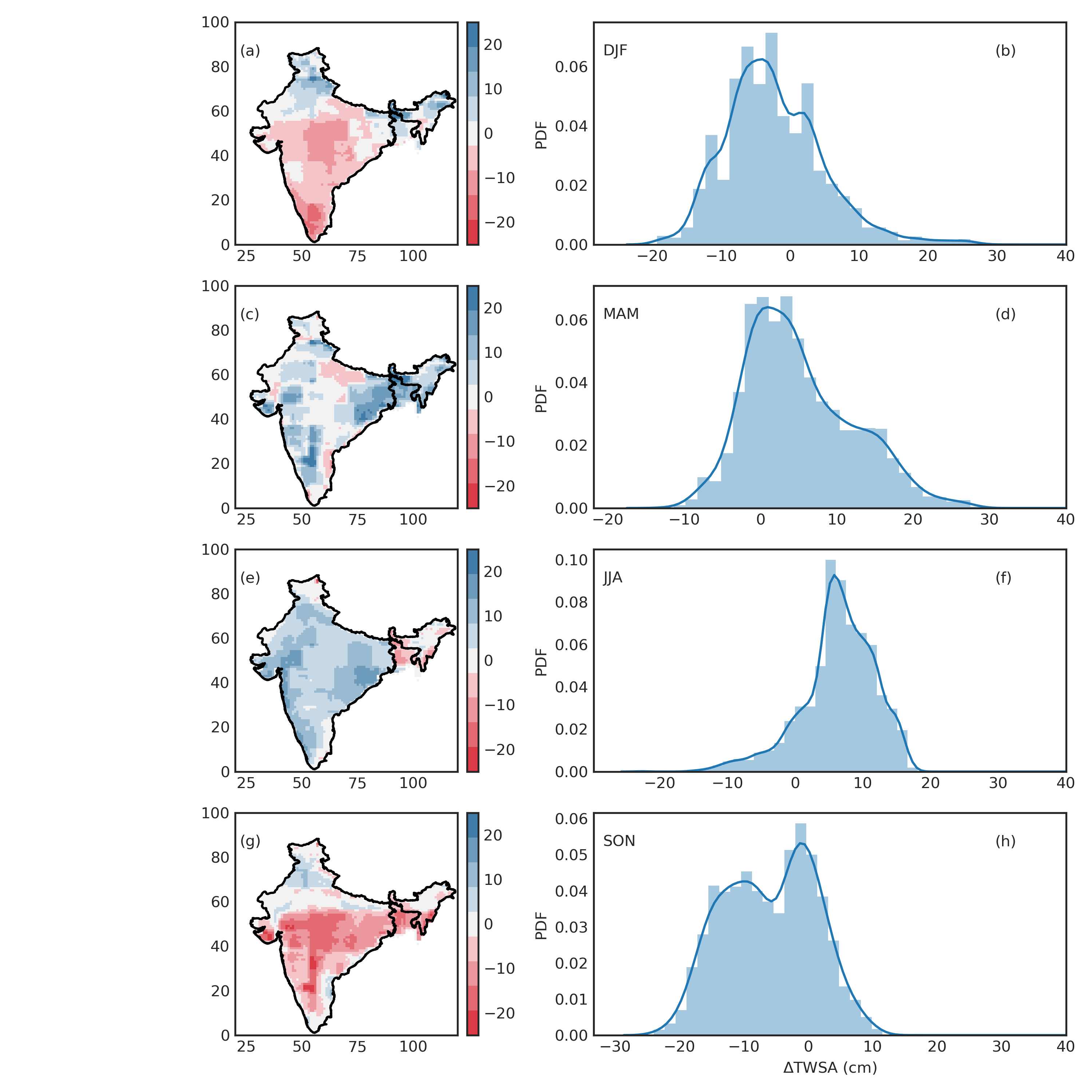
Figure 4 shows the seasonal patterns of , obtained by averaging the grid values over seasons Dec-Jan-Feb (DJF), Mar-Apr-May (MAM), Jun-Jul-Aug (JJA), and Sep-Oct-Nov (SON). Recall that represents the mismatch between NOAH and GRACE TWSA which, according to its definition in Eq. 2, tends to be negative in wet seasons and positive in dry seasons because of the missing SWS and GWS components in NOAH. Significant spatial and temporal variability can be observed in Figure 4. In particular, the histograms plotted on the right panel of Figure 4 suggest that in MAM (pre-monsoon dry season) and JJA (first part of monsoon season) is dominated by positive values with a mean value of 5.1 cm and 6.3 cm, respectively. The distribution in MAM is positively skewed, while it is negatively skewed in JJA, suggesting a transition from dry to wet season. In SON (late in monsoon season) and DJF (post-monsoon wet season), the pattern of is dominated by negative values with a mean of -6.0 cm and -2.3 cm. The negative values cover most of the regions in central and southern India. The distribution of in SON is also distinctively bimodal.
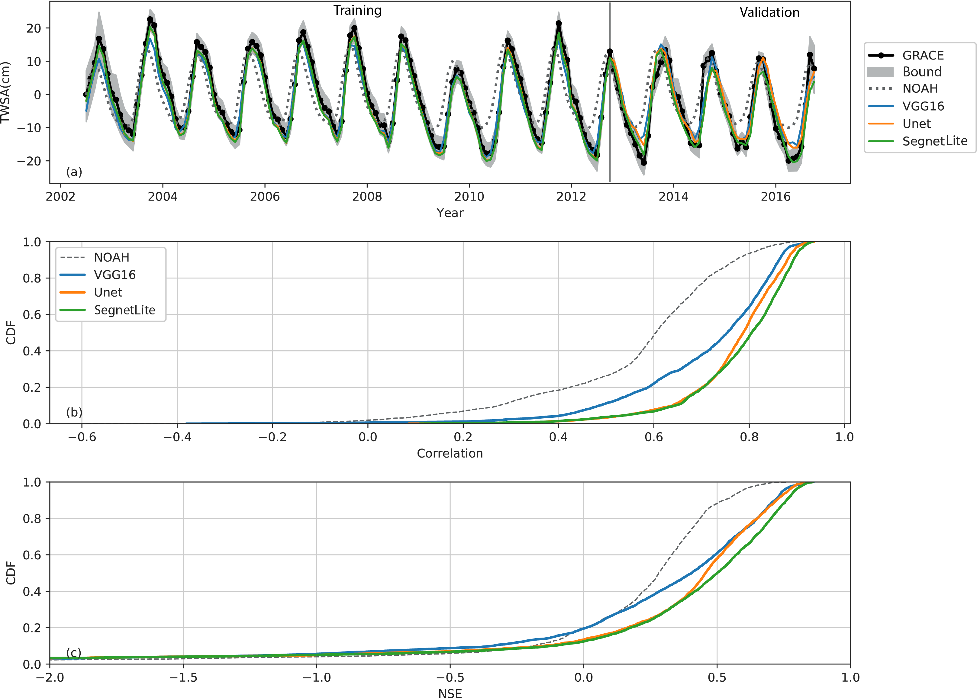
In the base case, we test the performance of VGG16, Unet, and SegnetLite models using only NOAH TWSA as the predictor (Table 1). The CNN-corrected TWSA is obtained by subtracting the predicted time series from the NOAH-simulated TWSA using Eq. 2. For comparison purposes, all models are trained over 60 epochs with a batch size of 5. Increasing the number of epochs further did not improve the results in our experiments. For each of the three CNN models, the correlation coefficient and NSE between the predicted and GRACE TWSA at both the country level and grid level are compared. This is because the GRACE research community is mostly interested on large-scale averaged results. Note that the actual training is done at the grid or pixel level, while the country-level statistics are calculated using grid-averaged TWSA time series. The country-level results are summarized in Table 1. For comparison, the metrics between the original NOAH TWSA and GRACE TWSA are reported in the first row.
At the country level, all CNN models achieved high correlation (>0.98) during training, which are all significantly higher than the correlation between the original NOAH TWSA and GRACE TWSA (0.78). For the testing period, the correlation values decrease slightly to about 0.94 on average, but are still higher than the correlation between the original NOAH and GRACE (0.83), or a 14% improvement on average. Because NOAH TWSA, GRACE TWSA, and are correlated, we applied Williams significance test (Williams, 1959) to test the improvement in correlation due to deep learning. The p-value of the Williams test is <0.002 for all three models (see Supporting Information (SI) S1), suggesting statistically significant improvement. It is worth noting that the correlation results obtained in this study are comparable to that obtained by Girotto et al. (2017), who reported that data assimilation increased the correlation between their model-simulated TWSA and GRACE to a country average of 0.96. Correlation coefficient measures the degree to which model and observations are related in phase, while NSE, a measure of predictive power, is sensitive to matches (or mismatches) of both magnitude and phase between the predicted and observed time series. In this case, the NSE value of the original NOAH TWSA is relatively low (0.6) for the training period. Figure 5a plots the base case results (solid lines in color), the GRACE TWSA (dark solid line with filled circles) and its error bound (shaded area), and the uncorrected NOAH TWSA (gray dashed line). For the training period, the plot suggests that the uncorrected NOAH TWSA underestimates most of the wet and dry events. In contrast, both Unet (orange line) and SegnetLite (green line) fit the wet and dry events well and are within the extent of the GRACE data uncertainty. The VGG16 model (dark blue solid line) underestimates the magnitudes of some wet events in 2002, 2003, and 2007.
During the testing period, we see several dry events, for example, the severe droughts in 2013 and 2016. In the literature, the dry events in 2014 and 2015 were attributed to monsoon rainfall deficits (Mishra et al., 2016). Again, the uncorrected NOAH underestimates the dry and wet events, especially the dry events. The SegnetLite model captures all dry events in 2013–2016 well, but slightly underestimates the 2014 and 2015 wet peaks. On the other hand, the VGG16 model captures most of the wet events, but underestimates dry events. The performance of Unet is in between. The average NSE improvement in the testing period is 0.87, or 52% improvement over the uncorrected NOAH TWSA. Figure 5a also suggests that even though the CNN models are trained at the grid level, they conserve mass at the country level. This is encouraging and may be attributed to the strong ability of CNN to learn multiscale spatial features and, therefore, preserve spatial continuity inherent in the input.
Figures 5b and 5c show the cumulative distribution function (CDF) of the pixel-wise, or grid-scale correlation coefficient and NSE between modeled TWSA and GRACE TWSA. The CDFs of all CNN-corrected results (solid lines in color) show a clear improvement over the original NOAH model (dashed line). Both Unet and SegnetLite give better performance than VGG16 and, in particular, the performance of SegnetLite is slightly better in the upper range of the correlation coefficient and NSE CDFs. The results thus far suggest that the mismatch pattern learned using NOAH TWSA as the base predictor can already help to correct the NOAH results significantly, both in magnitude and phase. On the basis of Table 1 and Figure 5, the SegnetLite model shows the best performance for the base case. The VGG16 model gives slightly worse results than the other two, probably because of the limited number of input feature maps it allows.
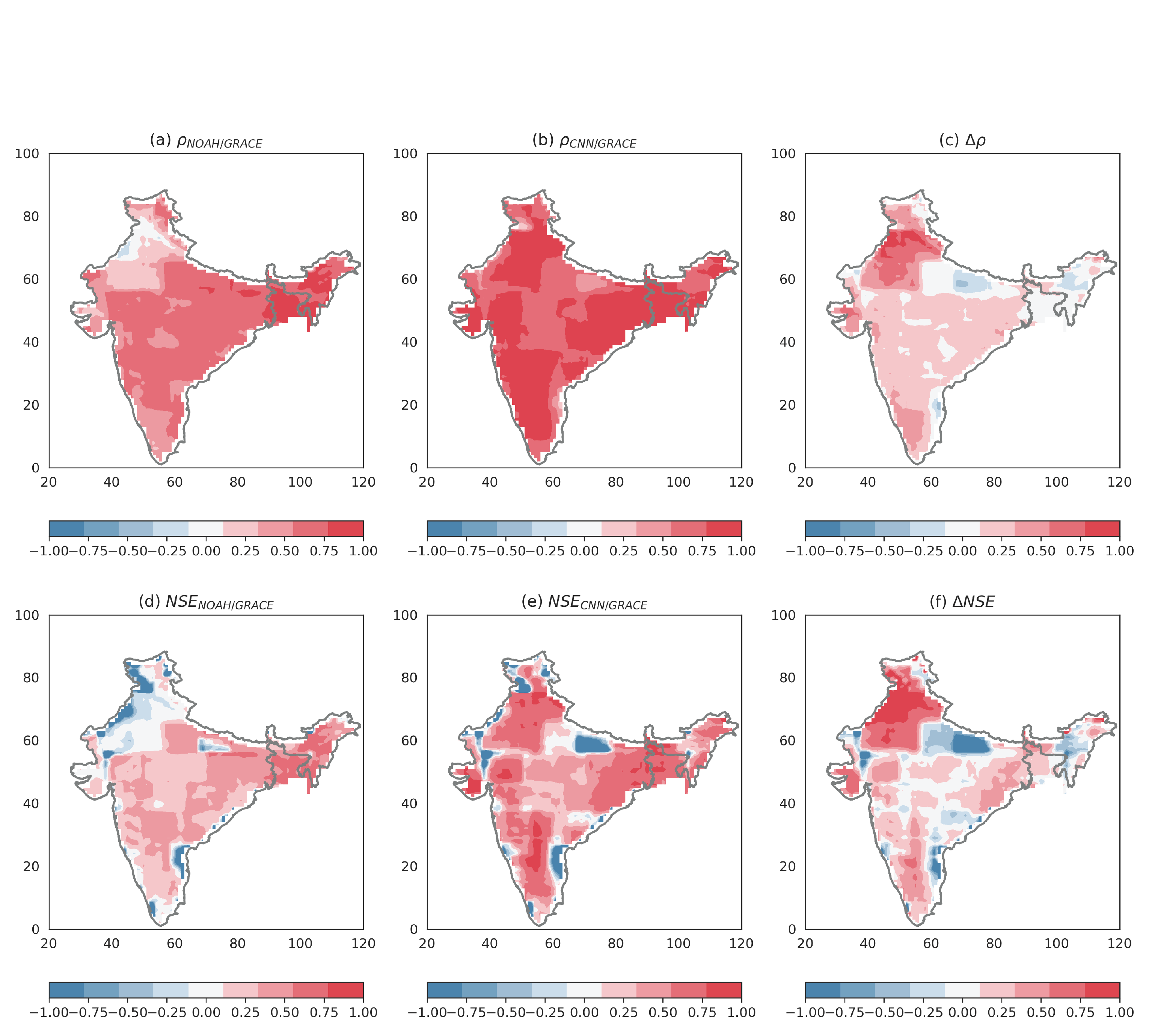
To help interpret the learned spatial patterns further, in Figure 6 we plot correlation and NSE maps corresponding to the uncorrected NOAH TWSA (6a, 6d), the SegnetLite model (6b, 6e), and improvements due to CNN correction, for the period 2002/04–2016/12 (6c, 6f). In general, higher correlation and NSE values are observed in southcentral and central India. The correlation improvement is the greatest in northwest and south India. The drier northwest India has been significantly affected by anthropogenic activities related to irrigation, whereas the wetter southmost part of the country is subject to bimodal precipitation pattern (Girotto et al., 2017), both are not resolved well in the current NOAH model. On the other hand, regional groundwater impact related to water withdrawal in northwest India has been confirmed by a number of previous GRACE studies (e.g., Rodell et al., 2009; Chen et al., 2014). Thus, the TWSA correction benefits the most in those areas. Nevertheless, isolated weak spots, especially on NSE maps, are found near the India-Nepal border (part of Ganges River Basin) and also in the Brahmaputra River Basin, where NOAH already gives good performance and the improvements by CNN are either insignificant or even deteriorated. The Himalayas region outside India’s north border may have negative impact on the learning because of sharp discontinuity in patterns. Similarly, the isolated weak spots along the Indian coast may also be related to the lack of continuity in patterns. Additional data may be necessary to constrain the CNN learning in those isolated spots. To give a sense of fitting quality, we show grid-level time series of NOAH TWSA, GRACE TWSA, and SegnetLite corrected TWSA at four selected pixel locations in SI S2. Two examples correspond to locations of significant NSE improvement (northwest India and southcentral India) and the other two examples show locations of performance deterioration (India-Nepal border and southern coastal area). SI S2 suggests that at the northwest India location, deep learning helps to improve the match of a downward trend observed by GRACE. SI S3 plots the same maps as shown in Figure 6 but for the testing period 2012/09–2016/12. In general, the same improvement patterns (i.e., and ) are observed over most of the region, except for north India where the effect due to correlation correction is little or none. The absolute NSE over northwest India is lower than that in Figure 6, although the NSE correction is still significant over most of the study region.
We performed additional tests for each type of CNN models by adding precipitation (P) and temperature (T) as predictors (Table 1). Results show that the additional predictors have little improvement over the base case (SI S4). Although P and T may include additional information (e.g., on SWS) not already included in the model, their effect may be limited by the resolutions of CNN models and GRACE observations, and by the strong seasonality of the study area. Nevertheless, P and T forcing may still be useful for reconstructing the TWS for other parts of the world.
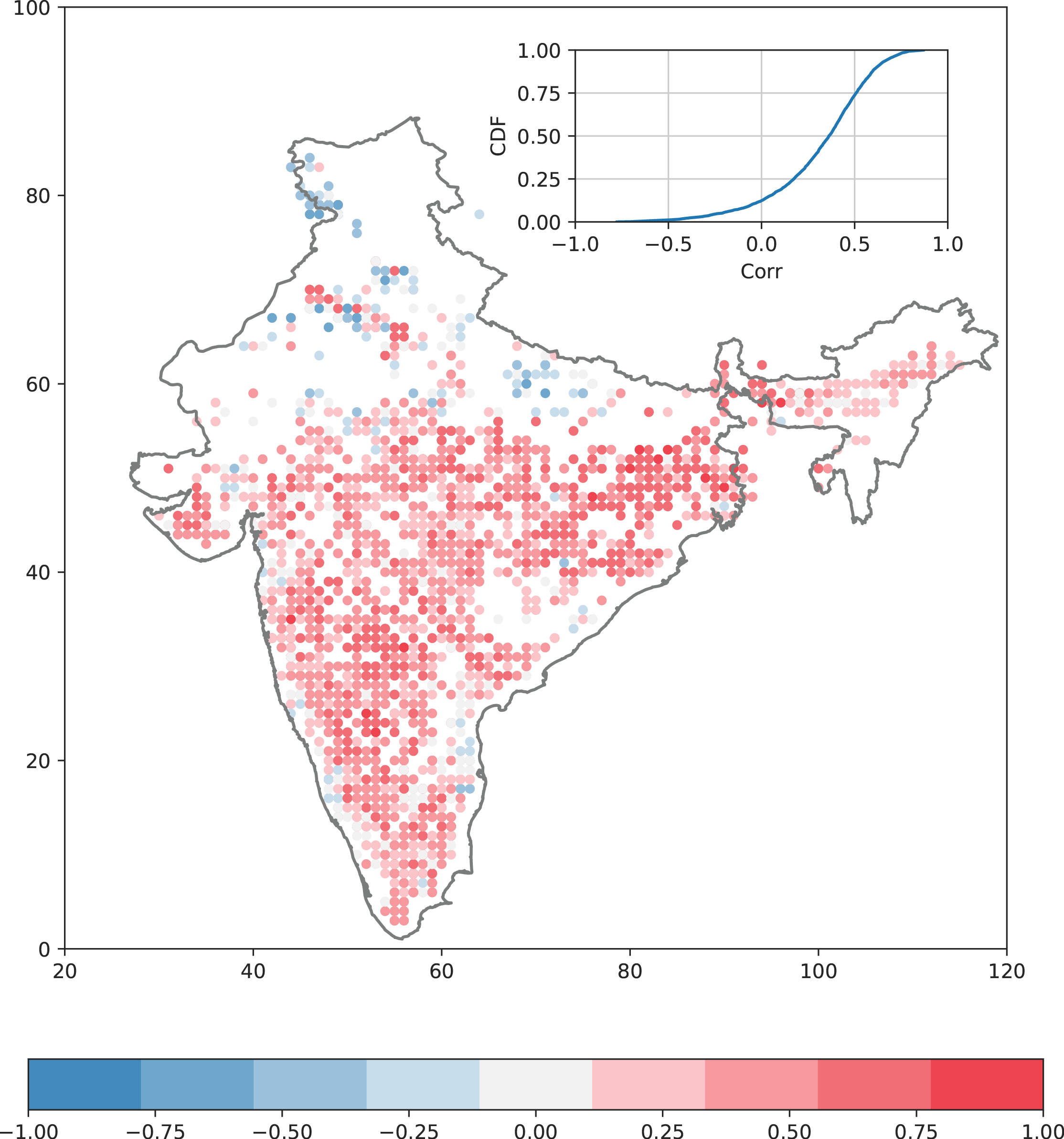
To further corroborate the learned patterns, we now compare to in situ groundwater storage anomalies (GWSA). As mentioned before, NOAH does not include SWS and GWS, while GRACE observes the total water column in space. Thus, the mismatch pattern should reflect the missing components, and is expected to correlate well with in situ GWSA wherever the TWSA is dominated by GWS. We assign groundwater wells to the nearest CNN model grid cells and then calculate the correlation coefficient between estimated by SegnetLite and in situ GWSA. Results are shown in Figure 7. Spatially, positive correlations are observed for most parts of India. The 50th percentile of correlation is about 0.4 (inset of Figure 7). The correlation is weaker in northwest India, the India-Nepal border, and along the southern coastal areas. The weaker correlation in northwest India is intriguing, given the dominance of groundwater in that region and strong correlation between the corrected NOAH and GRACE TWSA obtained for the same area, as shown in Figure 6b. One possible explanation is given by Girotto et al. (2017), who pointed out that groundwater used for irrigation in northwest India is “extracted primarily from deep aquifers, which are observed by GRACE, but not by the shallow in situ groundwater measurements.” Thus, the limitation of the in situ dataset needs to be kept in mind when interpreting the comparison results in Figure 7. For areas along the Indus River and Ganges River, the impact of surface water is relatively high (Getirana et al., 2017), which limits the proportion of GWSA in and weakens the correlation between and in-situ GWSA. Note in this comparison with the in situ GWSA, we mainly focus on analyzing the phase agreement because of the uncertainty of in situ GWSA magnitudes related to the uncertain specific yield.
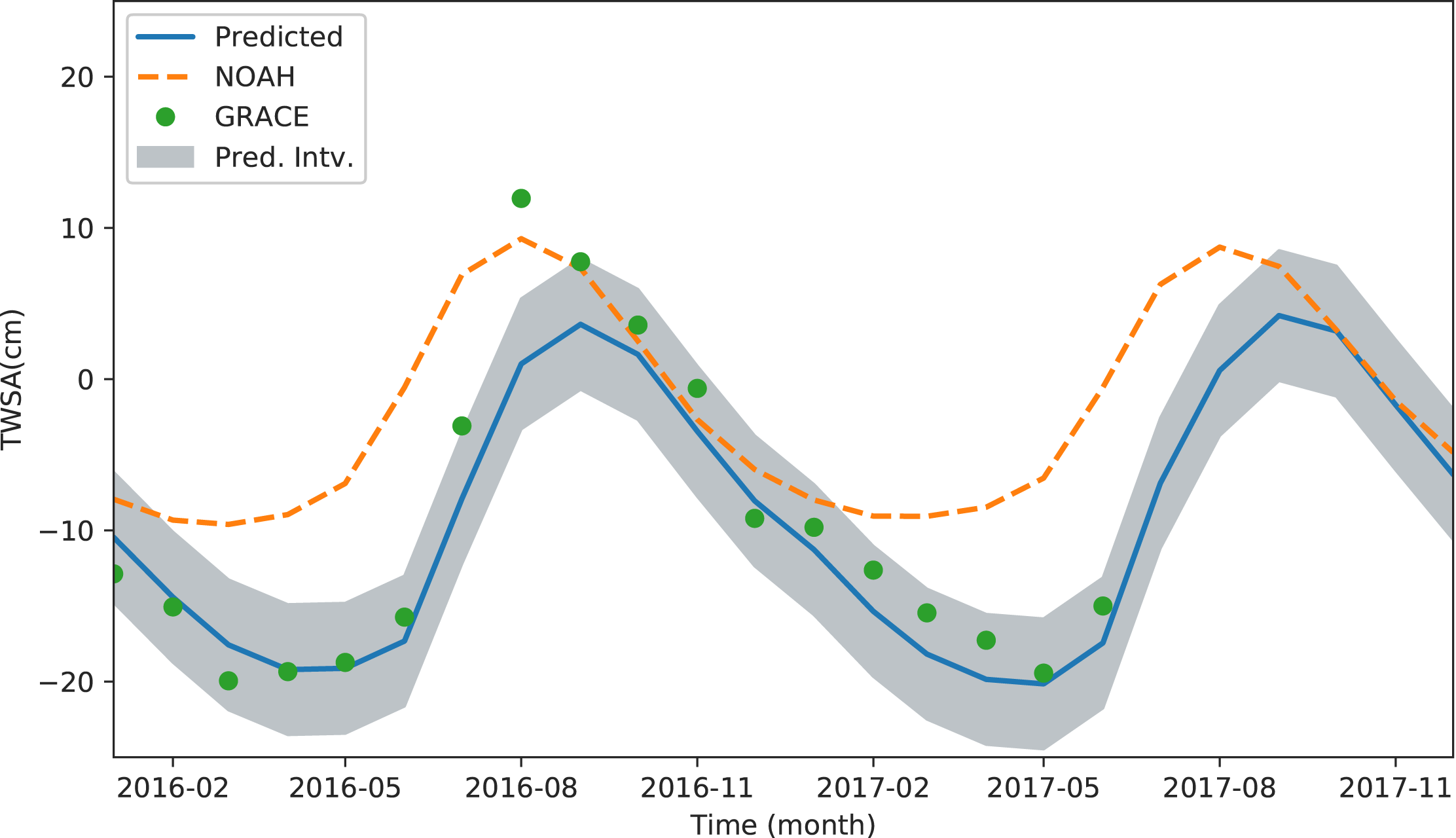
Finally, we apply the trained SegnetLite model to predict TWSA. Figure 8 shows the country-averaged TWSA for the period 2016–2017. The GRACE data (green filled circles) becomes unavailable after June 2017. Also, the GRACE data from 2017 is not part of the model training and testing. The 95% prediction interval is estimated using 1.96 RMSE, where the RMSE (~ 2.20 cm) is calculated by using the misfit of SegnetLite model on the training data. The plot suggests that the SegnetLite model captures the GRACE data well during the 2017 months that are not part of Figure 5a, demonstrating the potential use of this method for filling data gaps between GRACE and GRACE-FO.
5 Conclusion
In this study, we present a hybrid approach that combines physically-based modeling and deep learning to predict the spatial and temporal variations of TWS anomaly (TWSA). This is done by training CNN-based deep learning models (VGG16, Unet, and SegnetLite) to learn the spatial and temporal mismatch pattern between the TWSA simulated by a land surface model, NOAH, and that observed by GRACE, using which the NOAH-simulated TWSA is then corrected. The hybrid modeling approach is systematically demonstrated over India by using various performance metrics. In general, all deep learning models considered in this study are able to improve the NOAH TWSA significantly at both the country- and grid level, which is encouraging because we deal with a much smaller training sample size than those typically used in image classification problems. A correlation analysis between the learned patterns and the in situ groundwater storage anomaly (GWSA) shows good correlation between the two, suggesting the learned patterns effectively compensate for the missing groundwater storage in NOAH for many parts of the study area.
Our method presents an alternative for extrapolating TWSA time series outside the GRACE period. Our results also indicate the feasibility of using deep learning to perform spatial and temporal interpolation, which has long been a challenging problem in the geoscience literature. Compared to the conventional 4D variational or ensemble-based data assimilation techniques for fusing hydroclimatic data, major strengths of our hybrid approach include (1) the relatively few assumptions involved, especially with regard to parameterization of the spatial and temporal error distributions; (2) the capability to extract useful features at multiple scales, and (3) the capability to handle multiple data types with relative ease.
Deep learning algorithms evolve rapidly. In this study, we mainly considered three variants of CNN. In the literature, long short-term memory (LSTM) and recurrent neural networks (RNN) have been combined with CNN for spatiotemporal prediction problems (Shi et al., 2015; Fang et al., 2017). In addition, the grid resolution of our networks is relatively coarse. Finer resolution grids may be tested in the future to improve model fits.
Appendix
A.1 VGG-16
The pre-trained VGG16 model (i.e., weights) is obtained from the Keras package (Chollet et al., 2015). The VGG16 model design consists of a series of downsampling convolutional layers (3×3 filter, ReLU activation function), interlaced with max pooling layers (2×2) (Figure A.1). The number of filters increases gradually from 64 to 512, while the size of the feature map decreases from 128 to 8 (in pixels). At the end, the convolutional layers are flattened and connected to a fully connected layer before reshaped to the dimensions of the output layer (i.e., 128×128). Linear activation function is used for the output layer.
A.2 Unet model
The Unet model used in this work is adapted from the original design of Ronneberger et al. (2015), with modifications in the number of filters used. The model design belongs to a class of encoder-decoder architectures. The encoder part includes 5 consecutive downsampling steps, and the decoder part includes an equal number of upsampling steps. Each downsampling step involves 2 convolutional layers (using 3×3 filter and ReLU activation function), followed by a max pooling layer (2×2). For the encoder part, the number of filters in the convolutional layers increases from 32 to 512, while the dimensions of the feature maps decrease from 128×128 to 8×8. Each upsampling step involves (a) an upsampling step (2×2), (b) a concatenation step in which the feature maps from the same level of downsampling and upsampling paths are combined (dashed line in Figure A.2), and (c) two convolutional layers (using 3×3 filter and ReLU activation function). In its simplest form, upsampling repeats rows and columns to create a larger image (no trainable parameters). The inputs to the model include image stacks corresponding to one or more predictors, and the output of the model is the predicted mismatch, . A convolutional layer with linear activation function is used to generate the output.
A.3 SegnetLite model
Segnet is a deep CNN architecture introduced to perform semantic segmentation (Badrinarayanan et al., 2015). SegnetLite used in this work is a variant of the original Segnet, which uses a smaller number of encoding and decoding steps. In addition, no max-pooling is used and the upsampling layers in the original design are replaced by transpose convolution layers, which can be regarded as the reverse of convolutional operations and which increase the input dimensions like the upsampling does. However, transpose convolution layers introduce trainable parameters to learn the optimal upsampling parameters. The encoder part of SegnetLite consists of six convolution layers, with the number of filters increasing from 16 to 128, while the decoding part is symmetric and includes alternating concatenation and transpose convolution layers (Figure A.3). Similar to Unet, SegnetLite uses concatenation steps to combine feature maps from encoding and decoding steps at the same level. To generate the output layer, an upsampling layer is used to increase the decoder outputs to the output dimensions ( and is then passed through a convolutional layer as in the other two models.
Acknowledgments
The GRACE mascon product used in this study was downloaded from JPL (www.grace.jpl.nasa.gov). NOAH data were downloaded from NASA Earthdata site (http://earthdata.nasa.gov). Processing and numerical experiments were carried out on the Chameleon Cloud hosted by Texas Advanced Computing Center. A. Y. Sun and B. R. Scanlon were partially supported by funding from Jackson School of Geosciences, UT Austin. The authors are grateful to the Associate Editor and four anonymous reviewers for their constructive comments.
References
- Badrinarayanan et al. (2015) Badrinarayanan, V., A. Kendall, and R. Cipolla (2015), Segnet: A deep convolutional encoder-decoder architecture for image segmentation, arXiv preprint arXiv:1511.00561.
- Bhanja et al. (2016) Bhanja, S. N., A. Mukherjee, D. Saha, I. Velicogna, and J. S. Famiglietti (2016), Validation of grace based groundwater storage anomaly using in-situ groundwater level measurements in india, Journal of Hydrology, 543, 729–738.
- Bookhagen and Burbank (2010) Bookhagen, B., and D. W. Burbank (2010), Toward a complete himalayan hydrological budget: Spatiotemporal distribution of snowmelt and rainfall and their impact on river discharge, Journal of Geophysical Research: Earth Surface, 115(F3).
- Chen et al. (2014) Chen, J., J. Li, Z. Zhang, and S. Ni (2014), Long-term groundwater variations in northwest india from satellite gravity measurements, Global and Planetary Change, 116, 130–138.
- Chollet et al. (2015) Chollet, F., et al. (2015), Keras (2015).
- Ek et al. (2003) Ek, M., K. Mitchell, Y. Lin, E. Rogers, P. Grunmann, V. Koren, G. Gayno, and J. Tarpley (2003), Implementation of noah land surface model advances in the national centers for environmental prediction operational mesoscale eta model, Journal of Geophysical Research: Atmospheres, 108(D22).
- Fang et al. (2017) Fang, K., C. Shen, D. Kifer, and X. Yang (2017), Prolongation of smap to spatiotemporally seamless coverage of continental us using a deep learning neural network, Geophysical Research Letters, 44(21).
- Getirana et al. (2017) Getirana, A., S. Kumar, M. Girotto, and M. Rodell (2017), Rivers and floodplains as key components of global terrestrial water storage variability, Geophysical Research Letters, 44(20).
- Girotto et al. (2016) Girotto, M., G. J. De Lannoy, R. H. Reichle, and M. Rodell (2016), Assimilation of gridded terrestrial water storage observations from grace into a land surface model, Water Resources Research, 52(5), 4164–4183.
- Girotto et al. (2017) Girotto, M., G. J. De Lannoy, R. H. Reichle, M. Rodell, C. Draper, S. N. Bhanja, and A. Mukherjee (2017), Benefits and pitfalls of grace data assimilation: A case study of terrestrial water storage depletion in india, Geophysical Research Letters, 44(9), 4107–4115.
- Goodfellow et al. (2016) Goodfellow, I., Y. Bengio, A. Courville, and Y. Bengio (2016), Deep learning, vol. 1, MIT press Cambridge.
- Gupta and Nearing (2014) Gupta, H. V., and G. S. Nearing (2014), Debate—the future of hydrological sciences: A (common) path forward? using models and data to learn: A systems theoretic perspective on the future of hydrological science, Water Resources Research, 50(6), 5351–5359.
- He et al. (2016) He, K., X. Zhang, S. Ren, and J. Sun (2016), Deep residual learning for image recognition, in Proceedings of the IEEE conference on computer vision and pattern recognition, pp. 770–778.
- Houborg et al. (2012) Houborg, R., M. Rodell, B. Li, R. Reichle, and B. F. Zaitchik (2012), Drought indicators based on model-assimilated gravity recovery and climate experiment (grace) terrestrial water storage observations, Water Resources Research, 48(7).
- Humphrey et al. (2017) Humphrey, V., L. Gudmundsson, and S. I. Seneviratne (2017), A global reconstruction of climate-driven subdecadal water storage variability, Geophysical Research Letters, 44(5), 2300–2309.
- India Central Ground Water Board (2014) India Central Ground Water Board (2014), Ground water year book–india 2013-14, 76pp., Report.
- Jean et al. (2016) Jean, N., M. Burke, M. Xie, W. M. Davis, D. B. Lobell, and S. Ermon (2016), Combining satellite imagery and machine learning to predict poverty, Science, 353(6301), 790–794.
- Karpatne et al. (2017) Karpatne, A., G. Atluri, J. H. Faghmous, M. Steinbach, A. Banerjee, A. Ganguly, S. Shekhar, N. Samatova, and V. Kumar (2017), Theory-guided data science: A new paradigm for scientific discovery from data, IEEE Transactions on Knowledge and Data Engineering, 29(10), 2318–2331.
- Khaki et al. (2017) Khaki, M., I. Hoteit, M. Kuhn, J. Awange, E. Forootan, A. van Dijk, M. Schumacher, and C. Pattiaratchi (2017), Assessing sequential data assimilation techniques for integrating grace data into a hydrological model, Advances in Water Resources, 107, 301–316.
- Krause et al. (2005) Krause, P., D. Boyle, and F. Bäse (2005), Comparison of different efficiency criteria for hydrological model assessment, Advances in geosciences, 5, 89–97.
- LeCun (1989) LeCun, Y. (1989), Generalization and network design strategies, Connectionism in perspective, pp. 143–155.
- LeCun and Bengio (1995) LeCun, Y., and Y. Bengio (1995), Convolutional networks for images, speech, and time series, The handbook of brain theory and neural networks, 3361(10), 1995.
- LeCun et al. (2015) LeCun, Y., Y. Bengio, and G. Hinton (2015), Deep learning, nature, 521(7553), 436.
- Li et al. (2012) Li, B., M. Rodell, B. F. Zaitchik, R. H. Reichle, R. D. Koster, and T. M. van Dam (2012), Assimilation of grace terrestrial water storage into a land surface model: Evaluation and potential value for drought monitoring in western and central europe, Journal of Hydrology, 446, 103–115.
- Lo et al. (2010) Lo, M.-H., J. S. Famiglietti, P.-F. Yeh, and T. Syed (2010), Improving parameter estimation and water table depth simulation in a land surface model using grace water storage and estimated base flow data, Water Resources Research, 46(5).
- Long et al. (2014) Long, D., Y. Shen, A. Sun, Y. Hong, L. Longuevergne, Y. Yang, B. Li, and L. Chen (2014), Drought and flood monitoring for a large karst plateau in southwest china using extended grace data, Remote Sensing of Environment, 155, 145–160.
- Long et al. (2016) Long, D., X. Chen, B. R. Scanlon, Y. Wada, Y. Hong, V. P. Singh, Y. Chen, C. Wang, Z. Han, and W. Yang (2016), Have grace satellites overestimated groundwater depletion in the northwest india aquifer?, Scientific reports, 6, 24,398.
- MacDonald et al. (2016) MacDonald, A., H. Bonsor, K. Ahmed, W. Burgess, M. Basharat, R. Calow, A. Dixit, S. Foster, K. Gopal, D. Lapworth, et al. (2016), Groundwater quality and depletion in the indo-gangetic basin mapped from in situ observations, Nature Geoscience, 9(10), 762–766.
- Milzow et al. (2011) Milzow, C., P. E. Krogh, and P. Bauer-Gottwein (2011), Combining satellite radar altimetry, sar surface soil moisture and grace total storage changes for hydrological model calibration in a large poorly gauged catchment, Hydrology and Earth System Sciences, 15(6), 1729–1743.
- Miro and Famiglietti (2018) Miro, M. E., and J. S. Famiglietti (2018), Downscaling grace remote sensing datasets to high-resolution groundwater storage change maps of california’s central valley, Remote Sensing, 10(1), 143.
- Mishra et al. (2016) Mishra, V., S. Aadhar, A. Asoka, S. Pai, and R. Kumar (2016), On the frequency of the 2015 monsoon season drought in the indo-gangetic plain, Geophysical Research Letters, 43(23).
- Mooley and Parthasarathy (1984) Mooley, D., and B. Parthasarathy (1984), Fluctuations in all-india summer monsoon rainfall during 1871–1978, Climatic Change, 6(3), 287–301.
- Mukherjee et al. (2015) Mukherjee, A., D. Saha, C. F. Harvey, R. G. Taylor, K. M. Ahmed, and S. N. Bhanja (2015), Groundwater systems of the indian sub-continent, Journal of Hydrology: Regional Studies, 4, 1–14.
- Rodell and Famiglietti (2001) Rodell, M., and J. Famiglietti (2001), An analysis of terrestrial water storage variations in illinois with implications for the gravity recovery and climate experiment (grace), Water Resources Research, 37(5), 1327–1339.
- Rodell et al. (2004) Rodell, M., P. Houser, U. Jambor, J. Gottschalck, K. Mitchell, C. Meng, K. Arsenault, B. Cosgrove, J. Radakovich, and M. Bosilovich (2004), The global land data assimilation system, Bulletin of the American Meteorological Society, 85(3), 381–394.
- Rodell et al. (2009) Rodell, M., I. Velicogna, and J. S. Famiglietti (2009), Satellite-based estimates of groundwater depletion in india, Nature, 460(7258), 999.
- Ronneberger et al. (2015) Ronneberger, O., P. Fischer, and T. Brox (2015), U-net: Convolutional networks for biomedical image segmentation, in International Conference on Medical image computing and computer-assisted intervention, pp. 234–241, Springer.
- Russakovsky et al. (2015) Russakovsky, O., J. Deng, H. Su, J. Krause, S. Satheesh, S. Ma, Z. Huang, A. Karpathy, A. Khosla, and M. Bernstein (2015), Imagenet large scale visual recognition challenge, International Journal of Computer Vision, 115(3), 211–252.
- Scanlon et al. (2018) Scanlon, B. R., Z. Zhang, H. Save, A. Y. Sun, H. M. Schmied, L. P. van Beek, D. N. Wiese, Y. Wada, D. Long, and R. C. Reedy (2018), Global models underestimate large decadal declining and rising water storage trends relative to grace satellite data, Proceedings of the National Academy of Sciences, p. 201704665.
- Schmidhuber (2015) Schmidhuber, J. (2015), Deep learning in neural networks: An overview, Neural networks, 61, 85–117.
- Schumacher et al. (2016) Schumacher, M., J. Kusche, and P. Döll (2016), A systematic impact assessment of grace error correlation on data assimilation in hydrological models, Journal of Geodesy, 90(6), 537–559.
- Seneviratne et al. (2004) Seneviratne, S. I., P. Viterbo, D. Lüthi, and C. Schär (2004), Inferring changes in terrestrial water storage using era-40 reanalysis data: The mississippi river basin, Journal of climate, 17(11), 2039–2057.
- Seyoum and Milewski (2017) Seyoum, W. M., and A. M. Milewski (2017), Improved methods for estimating local terrestrial water dynamics from grace in the northern high plains, Advances in Water Resources, 110, 279–290.
- Shi et al. (2015) Shi, X., Z. Chen, H. Wang, D.-Y. Yeung, W.-K. Wong, and W.-c. Woo (2015), Convolutional lstm network: A machine learning approach for precipitation nowcasting, in Advances in neural information processing systems, pp. 802–810.
- Simonyan and Zisserman (2014) Simonyan, K., and A. Zisserman (2014), Very deep convolutional networks for large-scale image recognition, arXiv preprint arXiv:1409.1556.
- Sun (2013) Sun, A. Y. (2013), Predicting groundwater level changes using grace data, Water Resources Research, 49(9), 5900–5912.
- Sun et al. (2012) Sun, A. Y., R. Green, S. Swenson, and M. Rodell (2012), Toward calibration of regional groundwater models using grace data, Journal of Hydrology, 422, 1–9.
- Sun and Sun (2015) Sun, N.-Z., and A. Sun (2015), Model calibration and parameter estimation: for environmental and water resource systems, Springer.
- Swenson et al. (2003) Swenson, S., J. Wahr, and P. Milly (2003), Estimated accuracies of regional water storage variations inferred from the gravity recovery and climate experiment (grace), Water Resources Research, 39(8).
- Szegedy et al. (2015) Szegedy, C., W. Liu, Y. Jia, P. Sermanet, S. Reed, D. Anguelov, D. Erhan, V. Vanhoucke, and A. Rabinovich (2015), Going deeper with convolutions, in Proceedings of the IEEE conference on computer vision and pattern recognition, pp. 1–9.
- van Dijk et al. (2014) van Dijk, A. I., L. J. Renzullo, Y. Wada, and P. Tregoning (2014), A global water cycle reanalysis (2003–2012) merging satellite gravimetry and altimetry observations with a hydrological multi-model ensemble, Hydrology and Earth System Sciences, 18(8), 2955.
- Watkins et al. (2015) Watkins, M. M., D. N. Wiese, D. Yuan, C. Boening, and F. W. Landerer (2015), Improved methods for observing earth’s time variable mass distribution with grace using spherical cap mascons, Journal of Geophysical Research: Solid Earth, 120(4), 2648–2671.
- Werth and Güntner (2010) Werth, S., and A. Güntner (2010), Calibration analysis for water storage variability of the global hydrological model wghm, Hydrology and Earth System Sciences, 14(1), 59.
- Wiese et al. (2016) Wiese, D. N., F. W. Landerer, and M. M. Watkins (2016), Quantifying and reducing leakage errors in the jpl rl05m grace mascon solution, Water Resources Research, 52(9), 7490–7502.
- Williams (1959) Williams, E. J. (1959), Regression analysis, John Wiley & Sons, Incorporated.
- Zeiler et al. (2010) Zeiler, M. D., D. Krishnan, G. W. Taylor, and R. Fergus (2010), Deconvolutional networks.
- Zhang et al. (2016) Zhang, D., Q. Zhang, A. D. Werner, and X. Liu (2016), Grace-based hydrological drought evaluation of the yangtze river basin, china, Journal of Hydrometeorology, 17(3), 811–828.
| Model | Performance Metrics | |||
| Training | Testing | |||
| Corr | NSE | Corr | NSE | |
| 0.776 | 0.600 | 0.825 | 0.568 | |
| Base Case, only | ||||
| VGG16 | 0.986 | 0.925 | 0.944 | 0.862 |
| Unet | 1.0 | 0.948 | 0.938 | 0.868 |
| Segnet | 1.0 | 0.952 | 0.946 | 0.875 |
| and P | ||||
| VGG16-2 | 0.986 | 0.909 | 0.928 | 0.861 |
| Unet-2 | 1.0 | 0.969 | 0.941 | 0.880 |
| Segnet-2 | 1.0 | 0.961 | 0.943 | 0.880 |
| , P, and T | ||||
| VGG16-3 | 0.985 | 0.906 | 0.936 | 0.864 |
| Unet-3 | 1.0 | 0.961 | 0.939 | 0.876 |
| Segnet-3 | 1.0 | 0.977 | 0.945 | 0.889 |
Figure Captions
Figure 1. Map of study area (latitude: 7.75–47.75°, longitude: 60–100°), where India is bounded by the dark solid line. During training, data corresponding to the entire square area is used to reduce potential boundary effects and increase information content for training.
Figure 2. Illustration of the flow of information from GLDAS-NOAH and GRACE to the deep learning model. Here the observed mismatch is only used to train the CNN deep learning model and is no longer required after the model is trained. NOAH TWSA is the base predictor. Other predictors may include precipitation and temperature. The dashed arrow indicates that the same is also used for GRACE data assimilation studies.
Figure 3. General CNN model architecture used in this study. The input layer consists of the NOAH TWSA as the base input stack. Auxiliary predictors include precipitation and temperature. Each stack of input images include data from multiple time steps, . The operations include two stages for shallow and deep learning. The output is the predicted having the same dimensions as the input.
Figure 4. Spatial distribution (left panel) and histogram (right panel) of NOAH-GRACE mismatch, averaged over 4 seasons: (a), (b) DJF; (c), (d) MAM; (e), (f) JJA; and (g), (h) SON. Solid lines on histograms correspond to fitted PDFs. Map colors are scaled between (-25, 25) cm for visualization.
Figure 5.Comparison of (a) GRACE (dark solid line with filled circles), NOAH (gray dashed line), and CNN-corrected TWSA time series by VGG16 (blue), Unet (orange), and SegnetLite (green) for training and testing periods (separated by the thin vertical bar) at the country level; (b) and (c) CDFs of correlation coefficient and NSE between modeled TWSA (including both NOAH and CNN-corrected results) and GRACE at the grid level. Shaded area in (a) represents the total error bound of GRACE TWSA.
Figure 6. Grid-scale correlation coefficient maps between (a) NOAH-simulated TWSA and GRACE, (b) SegnetLite-corrected TWSA and GRACE, and (c) their differences; (d)—(f) the same maps but for NSE. For plotting purposes, all maps are scaled to [-1,1].
Figure 7. Correlation map between in situ GWSA and learned by SegnetLite model. Inset shows the CDF of correlation coefficient. The map coordinates are grid cell indices (from 0 to 127).
Figure 8. Country averaged TWSA (blue solid line) predicted for 2016–2017 by using the trained base SegnetLite model. Dashed line (orange) is the NOAH TWSA output, and also the input to the SegnetLite model. Filled circles (green) represent GRACE monthly data, and shaded area corresponds to 95% prediction intervals.
Figure A1. VGG16 model architecture.
Figure A2. Unet model architecture.
Figure A3. SegnetLite model architecture.