Same, Same But Different - Recovering Neural Network Quantization Error Through Weight Factorization

Abstract

Quantization of neural networks has become common practice, driven by the need for efficient implementations of deep neural networks on embedded devices. In this paper, we exploit an oft-overlooked degree of freedom in most networks - for a given layer, individual output channels can be scaled by any factor provided that the corresponding weights of the next layer are inversely scaled. Therefore, a given network has many factorizations which change the weights of the network without changing its function. We present a conceptually simple and easy to implement method that uses this property and show that proper factorizations significantly decrease the degradation caused by quantization. We show improvement on a wide variety of networks and achieve state-of-the-art degradation results for MobileNets. While our focus is on quantization, this type of factorization is applicable to other domains such as network-pruning, neural nets regularization and network interpretability.

1 Introduction

Early efforts in the field of deep learning have focused mostly on the training aspect of neural networks. The success of these efforts has led to widespread deployment of trained neural networks in data-centers (Park et al., 2018; Jouppi et al., 2017) and on embedded devices (Ignatov et al., 2018) where they are used for inference which in turn emphasized the need to make the inference phase more efficient. Quantization, which means conversion of the arithmetic used within the net from high-precision floating-points to low-precision integers, is an essential step for efficient deployment, however, quantization degrades network performance. Here, we follow the commonly used quantization scheme described in Jacob et al. (2017) but note that other schemes exist (Vanhoucke et al., 2011; Gupta et al., 2015; Courbariaux et al., 2014) to which our results apply as well. Briefly, integer quantization consists of approximating real values with intergers according to $x_{Q}=x/scale$ where $scale=(max(x)-min(x))/2^{N}$ and N is the number of bits used in the approximation. Each layer’s weights and activations are given a different scale according to their extremum values. The noise introduced by this limited precision approximation encapsulates a fundamental dynamic range-precision trade-off.

Existing approaches to decreasing induced degradation are ‘quantization-aware’ training (Jacob et al., 2017; Banner et al., 2018a; Zhou et al., 2017, 2018; McKinstry et al., 2018) and reducing the dynamic range of activations by clipping outliers (Migacz, 2017; Choi et al., 2018; Banner et al., 2018b). Training is a powerful method but it is time-consuming, hard to implement, and requires access to the original training dataset which might not always be available (e.g. when the user wishes to use an off-the-shelf pre-trained model). Clipping has limited effect since it only addresses noise from activation quantization.

In this paper, we propose a different approach. Instead of focusing on improving the quantization process itself, we explore equivalent weight arrangement that make the net less sensitive to quantization. An equivalent weight arrangements is a factorization that changes the weights of the networks without changing its function - i.e. for a given input, the network output remains the same. During quantization, the range of each layer is set by the channel with the largest absolute activation which we term the dominant channel. This single channel determines the noise in all other channels, many of which have smaller values. Therefore, amplifying these channels to match the dominant channel while compensating the change at the next layer can reduce the effect of the noise.

We begin by analyzing the noise introduced by quantization of weights and activations in terms of signal-to-quantization-noise ratio (SQNR). We inspect the effect of channel-scaling on SQNR and introduce an equalization procedure which, under some constraints, tries to scale each output channel such that its range matches that of the dominant channel. We show that equalization reduces the layer SQNR and then apply equalization iteratively layer-by-layer and empirically show that the overall post-quantization degradation of the network decreases. Since our approach can be a pre-processing step prior to quantization, it is fully compatible with other approaches that improve the quantization process. Nevertheless, an appealing aspect of our scheme is that for most nets it reduces the quantization induced degradation enough as to make quantization-aware training unnecessary and thus facilitates rapid deployment of quantized models.

The main contributions of this paper are:

• Inversely proportional factorization: we show the utility of weight factorization for the task of quantization. Future work can benefit by exploiting these factorizations in other settings. To the best of our knowledge this work is the first to both highlight and show the usefulness of inversely proportional factorizations.

• Equalization: we show that layers which have channels with similar ranges are less affected by quantization and we show how to transform a network closer to this ideal. We also perform a quantitative analysis of the effect of equalization on quantization noise and quantization induced degradation for a wide range of network architectures.

2 Previous Work

Equalization. Having channels with similar dynamic ranges motivated (Jacob et al., 2017) to use of Relu6 activations which were subsequently used in MobileNets (Howard et al., 2017). However, in practice, many channels remain un-clamped and the dynamic range strongly varies within a layer (Sheng et al., 2018). It was also observed (Krishnamoorthi, 2018) that having a scale for each channel of a layer greatly improves quantization performance. While effective for networks where most of the degradation stems from the quantization of weights, it doesn’t improve performance of networks that are degraded by the quantization of activation such as DenseNets (Huang et al., 2016).

Quantization Noise Analysis. The properties of noise induced by the quantization of both activations and weights were analyzed in Lin et al. (2015) focusing on the optimal bit width assignment to each layer across the network. We follow a similar analysis but focus on the dynamic ranges of individual channels within a layer. Sakr et al. (2017) gives an upper bound on the relationship between SQNR and network accuracy. An empirical disambiguation of the contributions of activation and weight noise to total degradation was given in Krishnamoorthi (2018) for several networks. The consensus of previous works seems to be that weight quantization is responsible for the bulk of degradation but we show the opposite for some common networks.

3 Theoretical Foundation

For a given network architecture there exist many weight assignments that result in networks that realize the same mapping from input to output. Thus, we are afforded with an important degree of freedom enabling us to choose assignments that have desirable properties for the task at hand. We show, that for a family of networks it is possible to gradually switch between equivalent assignments through the use of inversely proportional factorizations. These factorizations enable us to scale individual channels within a layer by any positive factor. We then analyze the source of quantization noise and show that by scaling channels we can improve the SQNR withing a layer. Our analysis is done for Convolutional Neural Networks (CNNs) but the same principles can apply to other types of nets as well. Since our focus is on trained networks we assume that batch-normalization (Ioffe & Szegedy, 2015) layers are always folded back to the preceding layer and we ignore them.

3.1 Channel scaling through inversely-proportional factorization

Consider a convolutional layer with kernel W, bias B, input X, and output Y. For notional simplicity we eschew convolutions and consider matrix multiplication. To this end we denote $X^{i,j}_{1\times(K_{x}\cdot K_{y}\cdot F_{in})},Y^{i,j}_{1\times F_{out}}$, the channel vectors when the kernel is centered on spatial position i,j within X,Y. We can then write the kernel as a matrix $W_{(K_{x}\cdot K_{y}\cdot F_{in})\times F_{out}}$ and the bias as a vector $B_{1\times F_{out}}$. The following two factorizations hold:

$$Y^{i,j} =(X^{i,j}C_{1})(C_{1}^{-1}W)+B$$ (1)

$$Y^{i,j}C_{2} =X^{i,j}(WC_{2})+(BC_{2})$$ (2)

where for both cases $C_{i}$ is a diagonal matrix with positive entries and $C_{i}^{-1}$ is its the inverse diagonal matrix. The first factorization scales the channels of the layer’s input and the second factorization scale the channels of layer’s output. We now consider a simple setting where $L1$ and $L2$ are two consecutive convolutionalal layers in a network. We assume that the activation function of $L1$, $A(\cdot)$, is homogeneous with degree 1 for positive numbers. That is, it satisfies equation 3.

$$A(\alpha\cdot x)=\alpha\cdot A(x)\ \ \ \forall\alpha>0$$ (3)

With this assumption, if $Y_{1}$ is the output of $L1$ and $X_{2}$ is the input to $L2$, the scaling of $Y_{1}$ results in a corresponding scaling of $X_{2}$. Combining all of the above we arrive to our main result - the post-activation output channels of $L1$ can be scaled by any positive factors by scaling the weights in the kernel and bias of $L1$ (1) and the output of the network will remain unchanged if we inversely scale the corresponding weight in $L2$ (2). We term this endomorphism an inversely-proportional factorization and it is shown schematically in Figure 1.

Figure 1: A schematic showing inversely proportional factorization in a pair of convolutional layers. An output channel $i$ in $K_{1}$, the kernel of $L1$, is scaled by a positive factor $c_{i}$. Assuming the activation function $A(\cdot)$ is homogeneous, the post activation channel is also scaled by $c_{i}$. All the weights in $K_{2}$, the kernel of $L2$ that interact with channel $i$ are inversely scaled. $Y_{2}$, the output of $L2$ remains unchanged. The bias terms were omitted for clarity.

With the exception of the last layer, we can scale the individual channels withing each layer in a full network by iteratively factorizing pairs of layers. Finally, we note that the commonly used ReLU(Nair & Hinton, 2010), PRelu(He et al., 2015a) and linear activations all satisfy the homogeneous property from equation (3). Thus our scheme is applicable to most commonly used CNNs.

3.2 Quantization Noise Analysis

Understanding the formation and propagation of quantization noise across the network is an essential step in the design of better quantization algorithms. In this section we analyze the effects of weight and activations quantization using the same two-layers setting depicted in Figure 1. We model the effect of limited precision by adding noise terms $\Delta W_{1}\in{\rm I\!R}^{K_{1}\times K_{1}\times F_{in1}\times F_{out1}}$, $\Delta W_{2}\in{\rm I\!R}^{K_{2}\times K_{2}\times F_{in2}\times F_{out2}}$, and $\Delta Y_{1}\in{\rm I\!R}^{F_{out1}}$ to $W_{1}$, $W_{2}$, and $Y_{1}$ respectively. The noisy model is shown in Figure 2. For simplicity we also assume that all the biases are zero and that all activations are linear.

Figure 2: A simple model showing the effects of quantization on two layers model. $\Delta W_{1}$, $\Delta W_{2}$, and $\Delta Y_{1}$ emulate the quantization effect.

We now show how each noise term affects the overall noise at the output of each layer. For a given tensor $T$ we denote $\hat{T}$ the noisy version of that tensor. In addition, we denote with $\tilde{T}^{\Delta N}$ the additive noise source to $T$ due to $\Delta N$. We start by calculating the output of the first layer

$$\begin{split}&\hat{Y_{1}}=X_{1}\circledast(W_{1}+\Delta W_{1})+\Delta Y_{1}\\ &=X_{1}*W_{1}+X_{1}\circledast\Delta W_{1}+\Delta Y_{1}\\ &\equiv Y_{1}+\tilde{Y_{1}}^{\Delta W_{1}}+\tilde{Y_{1}}^{\Delta Y_{1}}\end{split}$$ (4)

The output of the first layer has two noise sources. $\tilde{Y_{1}}^{\Delta W_{1}}$ is due to the interaction of the weight quantization noise with the input $X_{1}$ and $\tilde{Y_{1}}^{\Delta Y_{1}}$ is the intrinsic quantization noise. Assuming the noises are independent, their variance is:

$$\begin{split}E\left\{(\tilde{Y}_{1}^{\Delta W_{1}})^{2}\right\}&=K_{1}^{2}\cdot F_{in1}\cdot E\{(X_{1})^{2}\}\cdot E\{\Delta(W_{1})^{2}\}\\ E\left\{(\tilde{Y_{1}}^{\Delta Y_{1}})^{2}\right\}&=E\{\Delta Y_{1}^{2}\}\end{split}$$ (5)

For uniform quantization, the noise terms $\Delta W1,\Delta Y1$ distribution can be approximated as uniform, zero-centered, i.i.d processes (Lin et al., 2015; Marco & Neuhoff, 2005). Denoting by $W_{1}^{r}$, $Y_{1}^{r}$ the dynamic ranges of $W_{1}$, $Y_{1}$ we get

$$\Delta W1\sim U(-\frac{W_{1}^{r}}{2^{N+1}},\frac{W_{1}^{r}}{2^{N+1}})$$ (6)

$$\Delta Y1\sim U(-\frac{Y_{1}^{r}}{2^{N+1}},\frac{Y_{1}^{r}}{2^{N+1}})$$

The dynamic range of a tensor is determined by the extreme values across all the channels within it and so the noise distribution is determined by, at most, two channels - the channel with the largest value and the channel with smallest value. We term these channels the dominant channels and note that there is substantial variance between the extermum values of different channels. Next, we calculate the output of the second layer. Explicit calculation of $Y_{2}$ shows four noise sources, three are due to the quantization of $\Delta W_{1}$, $\Delta W_{2}$, $\Delta Y_{1}$, and one rooted in the multiplication of $Y_{1}^{\Delta W_{1}}$, $Y_{1}^{\Delta Y_{1}}$ by $\Delta W_{2}$. The last component can be neglected in most practical scenarios and the variances of the others are

$$\begin{split}E\left\{(\tilde{Y_{2}}^{\Delta W_{1}})^{2}\right\}&=\left(\sum W_{2}^{2}\right)\cdot E\left\{(\tilde{Y_{1}}^{\Delta W_{1}})^{2}\right\}\\ E\left\{(\tilde{Y_{2}}^{\Delta Y_{1}})^{2}\right\}&=\left(\sum W_{2}^{2}\right)\cdot E\left\{(\tilde{Y_{1}}^{\Delta Y_{2}})^{2}\right\}\\ E\left\{(\tilde{Y_{2}}^{\Delta W_{2}})^{2}\right\}&=K_{2}^{2}\cdot F_{in2}\cdot E\{(Y_{1})^{2}\}\cdot E\{(\Delta W_{2})^{2}\}\\ \end{split}$$ (7)

3.3 Effect of inversely-proportional factorization on SQNR

We use SQNR to quantify the effect of the quantization noise.

$$SQNR_{Y}\equiv\frac{E\left\{Y^{2}\right\}}{E\left\{(Y-\hat{Y})^{2}\right\}}=\frac{E\left\{Y^{2}\right\}}{E\left\{\tilde{Y}^{2}\right\}}$$ (8)

We calculate $SQNR_{Y1}$ and $SQNR_{Y2}$, the SQNRs at the outputs of layer 1 and 2 respectively, by plugging (5),(7) into (8).

$$SQNR_{Y1}=\frac{E\left\{Y_{1}^{2}\right\}}{E\left\{(\tilde{Y_{1}}^{\Delta W_{1}}+\tilde{Y_{1}}^{\Delta Y_{1}})^{2}\right\}}$$ (9)

$$SQNR_{Y2}=\frac{E\left\{Y_{1}^{2}\right\}}{E\left\{(\tilde{Y_{2}}^{\Delta W_{1}}+\tilde{Y_{2}}^{\Delta Y_{1}}+\tilde{Y_{2}}^{\Delta W_{2}})^{2}\right\}}$$

We now show how inversely proportional factorization affects the SQNR of both layers. We start by looking at the effect on the signal components. We denote the scaling vector with $C\in{\rm I\!R}^{F_{out1}}$ and the scaled version of tensor $T$ by $T^{\prime}$. For simplicity, since scaling the whole layer by a constant has no effect on the SQNR, we can assume without loss of generality that $C\geq 1$. Therefore, we can say that all channels in $Y_{1}$ are either amplified or unchanged. In addition, we showed in Section 3.1 that the factorization has no effect on $Y_{2}$. Thus for the signal components we have

$$E\{(Y_{1}^{\prime})^{2}\} \geq E\{(Y_{1})^{2}\}$$ (10)

$$E\{(Y_{2}^{\prime})^{2}\} =E\{(Y_{2})^{2}\}$$

Amplifying the channels of $Y_{1}$ haphazardly might increase the layer’s extremum values which will increases the variance of the noise sources $\Delta W_{1}$, $\Delta Y_{1}$ (6). On the other hand, amplification $Y_{1}$ is compensated by attenuation of $W_{2}$ which may only decrease the variance of $\Delta W_{2}$ if it results in a reduction of $W_{2}$’s extremum values. Thus for the noise sources we have

$$E\{(\Delta W_{1}^{\prime})^{2}\} \geq E\{(\Delta W_{1})^{2}\}$$ (11)

$$E\{(\Delta Y_{1}^{\prime})^{2}\} \geq E\{(\Delta Y_{1})^{2}\}$$

$$E\{(\Delta W_{2}^{\prime})^{2}\} \leq E\{(\Delta W_{2})^{2}\}$$

We now make the crucial assumption that the channels of $Y_{1}$ are amplified in such a manner that the variances of $\Delta W_{1}$, $\Delta Y_{1}$ remain unchanged while the variance of $\Delta W_{2}$ decreases. Under these assumptions, $\tilde{Y_{1}}^{\Delta W_{1}}$, $\tilde{Y_{1}}^{\Delta Y_{1}}$ are unaffected by the amplification of $Y_{1}$ and we get that

$$SQNR^{\prime}_{Y1}\geq SQNR_{Y1}$$ (12)

The effect on $SQNR_{Y2}$ (9) is more tricky. $E\left\{(\tilde{Y2}^{\Delta W1})^{2}\right\}$, $E\left\{(\tilde{Y2}^{\Delta Y1})^{2}\right\}$ are decreased by the attenuation of $W_{2}$. What happens to $E\left\{(\tilde{Y_{2}}^{\Delta W_{2}})^{2}\right\}$ depends on $E\{(Y_{1})^{2}\}\cdot E\{(\Delta W_{2})^{2}\}$, i.e. whether the amplification of $Y_{1}$ is more dominant than the attenuation of $\Delta W_{2}$. Thus there is no guarantee that $SQNR_{Y2}$ improves. Undaunted, in the next section we present a greedy algorithm that through iterative application of inversely-proportional factorization improves the SQNR across the network and reduces the post-quantization degradation.

4 Equalization Algorithm

Building on the analysis in Section 3 we propose two algorithms designed around the idea of applying a pre-quantization factorization that increases the energy of channels without changing the variance of the noise. This is achieved by amplifying non-dominant channels such that their extremum values are matched with those of the dominant channels. As shown in Figure 3, these algorithms tends to equalize the channels’ energy and therefore got the name channel equalization.

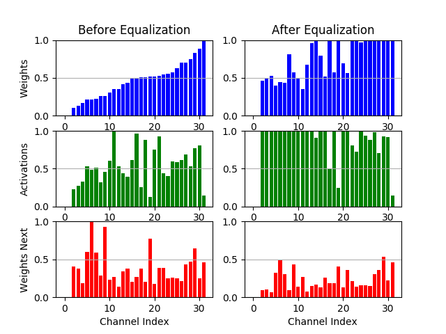
(a) One Step Equalization

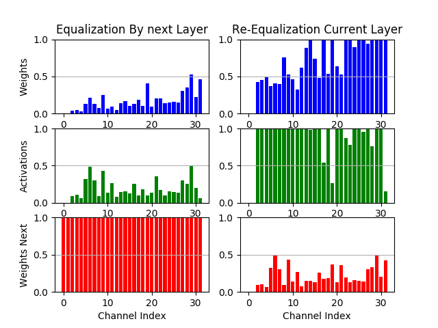
(b) Two Steps Equalization

Figure 3: Example of the effect of channel equalization on the two layers model. Each bar indicates the maximum values of a channel. The blue graphs show the data for weights, the green for the activations, and the red the weights of the successor layer. Figure (a) demonstrates the one step algorithm. On the left is the initial state and on the right is the state after equalization. Figure (b) demonstrates the two steps algorithm. On the left is the state after is the next layer weights equalization and on the right is the final state

4.1 One-Step Equalization

Algorithm 1 One Step Equalization

1:  while 1 do

2:     $layer\leftarrow getNextLayer()$

3:     if layer is last layer then

4:        return

5:     end if

6:     $kerOutChMax\leftarrow getKerOutChMax(layer)$

7:     $actOutChMax\leftarrow getActOutChMax(layer)$

8:     $kerOutMax\leftarrow max(kerOutChMax)$

9:     $actOutMax\leftarrow max(actOutChlMax)$

10:     $kerScale\leftarrow\frac{kerOutMax}{kerOutChMax}$

11:     $actScale\leftarrow\frac{actOutMax}{actOutChMax}$

12:     $scale\leftarrow min(kerScale,actScale,S_{max})$

13:     $scaleLayer(layer,scale)$

14:  end while

Algorithm 1 explains a simple, one-step channel equalization method. We assume that the network can be represented as direct acyclic graph with layers being represnted by nodes and that it is topologicaly sorted. The algorithm is then applied iteratively beginning at the first layer(node) and continues until we reach all of the network’s output layers. At each iteration the layer’s channels are equalized by employing inversely-proportional factorization with its successor layers. A layer is eligible to be equalized only once all of its predecessor layers were equalized. The function $getNextLayer()$ returns the next layer. The functions $getKerOutChMax(layer)$ and $getActOutChMax(layer)$ return the maximum values per channel for the weights and activation respectively. Each one of them results in a vector of length $F_{out}$. For each channel, we calculate the ratio between the layer’s extermum and the channel’s extremum for the activations and weights, these ratios are defined as the activation and weight scales. When a layer is scaled, each channel is scaled by the minimum between the activation and weight scales. We further limit the scale by a pre-defined maximum to prevent the over-scaling of channels with small activation values. $scaleLayer(layer,scale)$ is the scaling of the layer and its successors according to (1), (2). It is easy to see that the maximum values of the weights and the activation post equalization won’t change and that all the scales are $\geq 1$.

An example of the results of one-step equalization on the channel scales within a layer is shown in Figure 3(a). We see that, post equalization, channels have much less variance in scales which in turn implies that they tend to have similar energy. As explained in section 3.3 for each iteration there is no guarantee that $SQNR_{Y2}$ improves but in most cases we witnessed that it did. Moreover, even if the $SQNR_{Y2}$ decreases it will improved in next iteration when the channel of $Y_{2}$ will be equalized.

4.2 Two Steps Equalization

We define optimal equalization (OE) as the state where the extremum values of all the channels are equal. OE can be done in terms of weights only, activations only or both. OE for activations or weights can always be achieved but equalization of one will be sub-optimal for the other. OE for both, on the other hand, is out of reach in most cases because we have only one scale per channel. The two steps equalization tries to make a step toward the optimal OE.

Algorithm 2 Two Steps Equalization

1:  while 1 do

2:     $layer\leftarrow getNextLayer()$

3:     if layer is last layer then

4:        return

5:     end if

6:     $sucInChMax\leftarrow getSucInChMax(layer)$

7:     $sucInMax\leftarrow max(sucInChMax)$

8:     $kerOutChMax\leftarrow getKerOutChMax(layer)$

9:     $actOutChMax\leftarrow getActOutChMax(layer)$

10:     $kerOutMax\leftarrow max(kerOutChMax)$

11:     $actOutMax\leftarrow max(actOutChMax)$

12:     $kerScale\leftarrow\frac{KerOutMax}{kerOutChMax}\cdot\frac{sucInChMax}{sucInMax}$

13:     $actScale\leftarrow\frac{actOutMax}{actOutChMax}\cdot\frac{sucInChMax}{sucInMax}$

14:     $scale=min(kerScale,actScale,S_{max})$

15:     $scale=scale/min(scale)$

16:     $scaleLayer(layer,scale)$

17:  end while

Algorithm 2 explains the two steps equalization process. The basic idea is to diminish the layers extremum values before the equalization. This is done by applying proportionally-inverse factorization in reverse - we attenuate the channels of the first layer and compensate by amplifying the values of the second layer. To avoid increasing the weight noise in the second layer the compensating amplification is not allowed to change the extremum values of the second layer. This is done by using the function $getSucInChMax$ that returns the maximum per input channel of the successor layer weights. Dividing each channel by $\frac{sucInChMax}{sucInMax}$ will equalize the next layer and attenuate all the channels in the current layer. The second step of the algorithm is the same as in the one-step equalization. At the end of the algorithm we normalized all the scales so they will all be $\geq 1$. Figure 3(b) shows an example of two steps equalization. We can see that the channels are equalized a little bit better and that the maximum value of the next layer is lower. Therefore, we can expect the noise in the network after this equalization will be attenuated and indeed our tests showed that this algorithm can produce better channel equalization. Our intuition is that if a dominant channel can be attenuated than it means that the weights of second layer multiplying it are small. In other words - before the factorization the second layer was ”naturally” attenuating the channel, signaling that its scale is too large compared to the other channels. In a limited precision setting it is important that this ”gain control” be done beforehand since quantization is adversely affected by channels with outlier scales.

5 Experiments and Results

In this section we perform experiments analyzing the performance of our proposed algorithms. We first verify our analysis in previous sections by measuring the noise across test networks with and without equalization. We then show that a reduction in noise translates to a reduction in the post-quantization degradation of classifier networks trained on the ImageNet dataset(Russakovsky et al., 2015) and finally we show that our algorithm can also be applied to MobileNets(Howard et al., 2017) with some modifications. In all our tests we used layer wise quantization. Activations were encoded using 8-bit unsigned integers and weights were encoded using 8-bit integers. Biases were encoded using 16-bits integers. We used passive quantization, meaning that no retrain was used and there is no need for labeled data. For all experiments we extract the activation extremum values using 64 images.

5.1 SQNR measurements

We designed a test that shows the noise of each layer separately. Moreover, the test can differentiate between activations and weights noises. For each layer we measured three quantities: the layer output where only the weights are quantized ($Y_{1}+\tilde{Y_{1}}^{\Delta W_{1}}$), the layer output where only the activations are quantized($Y_{1}+\tilde{Y_{1}}^{\Delta Y1}$), and the layer output where both are quantized ($\hat{Y_{1}}$). To measure the noise we compared these quantities to those of the original full precision layer output.

We measured the SQNR of each layer and compared it to the one predicted by (5) to verify our assumptions. The results of this experiment are shown in in Figure 4 for ResNet-152(He et al., 2015b) and Inception-V3(Szegedy et al., 2015). The results show good agreement between predicted and measured noise.

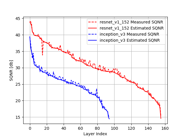
Figure 4: Noise estimation verification, A Comparison between the estimated SQNR according to (5) and measured SQNR. The layer index is sorted by the estimated SQNR from largest to smallest.

We now analyze the quality of our two-steps equalization algorithm. To that end we look at a simple setting where only the weight or only the activations are quantized. For weight quantization, we compare $SQNR_{W1}\equiv\sum(W_{1})^{2}/\sum(\Delta W_{1})^{2}$, a measure of how well the layers weights are equalized to the weight OE. And for activation quantization, we compare $SQNR_{Y1}\equiv\sum(Y_{1})^{2}/\sum(\Delta Y_{1})^{2}$ , a measure of how well the layers output channels are equalized, to the activation OE. This gives us an idea how far we are from the overall OE of both activations and weights. Figure 5 shows the results of this comparison on Inception-V3. We see that the method improves significantly the SQNR of the activations and almost reached the performance of the OE. For weights, the effect is smaller and the gap to the OE is larger.

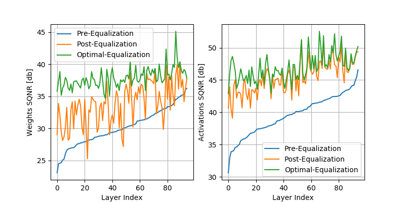
Figure 5: A comparison to the optimal SQNR. Demonstrating the effect of equalization algorithm on the SQNR for inception-V3. The figure shows how the algorithm tries to close the gap between the original state and optimal equalization. In these graphs the energy of the signal is measured and noise is estimated based on a uniform distribution assumption. The layer index is sorted by the estimated SQNR from largest to smallest.

Finally, we measured the effect of equalization on noises throughout the network. We measured the SQNR in three cases: without equalization, with one- and two-steps equalization. Observing the results, as shown on Figure 6, several conclusions can be drawn:(1) overall the SQNR is improved by equalization (2) The greedy nature of the algorithm means that for some intermediate layers the weight induced SQNR decreases. This is due to the fact that weight induced noise is increased when the layer input is amplified.

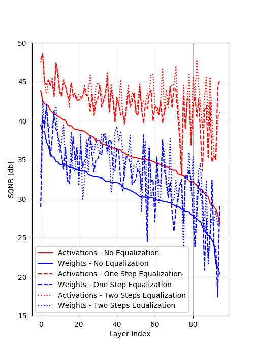
(a) Matched

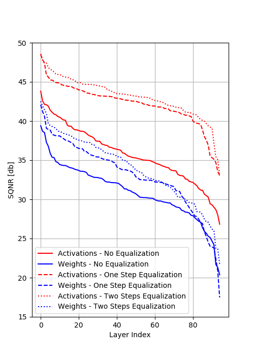
(b) Sorted

Figure 6: Noise measurement across the network for Inception-V3. Measure the activation SQNR $\sum(Y_{1})^{2}/\sum(\tilde{Y}_{1}^{\Delta Y_{1}})^{2}$ and weights SQNR $\sum(Y_{1})^{2}/\sum(\tilde{Y}_{1}^{\Delta W_{1}})^{2}$ for three cases: pre-equalization, post one step equalization, and post two steps equalization. In figure (a), for better visibility, the layers are sorted by pre-equalization SQNR values. In figure (b), for even better visibility, the post equalization lines are sorted as well.

5.2 ImageNet Quantization Performance

We now show that the overall reduction in SQNR achieved by the equalization algorithms results in improved performance of the quantized networks. Table 1 summarizes our results. We compared the classification performances of the quantized networks to their floating point version. Equalization improves quantization performance for almost all nets and for some, like inception-V1 (Szegedy et al., 2014) and DenseNet121 , a considerable improvement is observed. An examination of these networks revealed layers which suffer from an extreme imbalance between the channels. As we showed, this significantly increase the noise within the layer, triggering an avalanche effect throughout the network. Equalization eliminates this effect and enables good performance post quantization. Overall we see that two-steps equalization gives better performance than one-step equalization.

Figure 6 shows that the noise stemming from activation quantization is always reduced while the noise stemming from weight quantization occasionally increases after equalization. To quantify the effect we have on both noise sources we repeated the performance measurements for weights-only and activations-only quantization. We see that equalization has a positive effect for both scenarios and that which noise term is dominant is network dependent. For example, for the Inception architectures, weights quantization is dominant, while for ResNet-152 and DenseNet activation quantization is dominant. In addition, our results indicate that the total degradation $\approx$ weight degradation + activation degradation.

MobileNet is a challenging architecture for quantization and many passive quantization schemes result in large degradation (Jacob et al., 2017; Lee et al., 2018). It also employs ReLU6(Jacob et al., 2017) activations which require special treatment for the equalization algorithm to work since it does not satisfy (3).

Table 1: A comparison of the performance of the two proposed algorithms. For each network we tabulate the post-quantization degradation without equalization and with one- and two-steps equalization. The degradation is measured relative to the networks top-1 accuracy which is estimated using the full ILSCRC2015 validation set of 50K images. For Resnet-152 and Inception-V3 we also measure the degradation when only the weights or activations are quantized. To facilitate reproducibility we used open source pre-trained networks. All networks are taken from TF-slim models (TF-slim, ) with the exception of DenseNet(GitHub, )

Network Name	Original Top-1 accuracy	No Equal	One Step Equal	Two Steps Equal
Weights and Activations Quantization
ResNet-V1-50	$75.2\%$	$0.25\%$	$0.38\%$	$0.25\%$
ResNet-V1-152	$76.8\%$	$1.27\%$	$0.80\%$	$0.78\%$
Inception-V3	$77.9\%$	$0.66\%$	$0.47\%$	$0.35\%$
Inception-V1	$69.8\%$	$2.23\%$	$0.41\%$	$0.39\%$
DenseNet-121	$74.3\%$	$5.78\%$	$0.42\%$	$0.35\%$
Weights Quantization Only
ResNet-V1-152	$76.8\%$	$0.23\%$	$0.19\%$	$0.16\%$
Inception-V3	$77.9\%$	$0.55\%$	$0.36\%$	$0.32\%$
Activations Quantization Only
ResNet-V1-152	$76.8\%$	$0.98\%$	$0.66\%$	$0.62\%$
Inception-V3	$77.9\%$	$0.09\%$	$0.03\%$	$0.05\%$

One-step equalization can be used almost without change if it only amplifies channels with extremum activation value below 6. One-step equalization gives limited improvement (Table 2). To enable Two-steps equalization we disable the division by $min(scale)$ at the end of algorithm 2 and in doing so allow the algorithm to attenuate channels ($C<1$). However, to prevent significant modification to the full-precision network results, we limit the attenuation to 70% of the original range. This method shows negligible effect on the full-precision network but shows a significant improvement for the quantized network (Table 2).

In addition, we found that due to the use of depthwise convolutions which have a small number of weights in each kernel the mean of the quantized weights might be different from the original value which results in a shift of the distribution. As a remedy to this problem we use knowledge distillation (Hinton et al., 2015) and fine-tune only the biases to compensate for the shift so that the distribution means are the same for both the original and quantized network. Since only the biases are being updated 1000 unlabeled images are all that is needed and the fine-tuning process is very short. Used in conjunction with equalization we get competitive results (Table 2) with the state-of-the art (Jacob et al., 2017; Lee et al., 2018; Krishnamoorthi, 2018; Sheng et al., 2018; Google, ). However, our result is unique in the following regards: it doesn’t require channel-wise quantization which has significant overhead for hardware implementation as well as additional storage requirements. It uses only $\sim 1000$ unlabeled images allowing it to be used with off-the-shelf pre-trained models and the quantization process is simple and very fast to implement.

Table 2: MobileNet degradation of the different quantization schemes compared to the floating point implementation. All networks are taken from TF-slim models (TF-slim, ).

Net Version	No Equal	One Step Equal	Two Steps Equal	Bias Only	Equal+ Bias
V1-1.0	$7.89\%$	$6.12\%$	$3.2\%$	$1.3\%$	$0.95\%$
V2-1.0	$42.68\%$	$4.07\%$	$2.1\%$	$1.5\%$	$0.61\%$
V2-1.4	$8.06\%$	$6.21\%$	$1.9\%$	$1.4\%$	$0.55\%$

6 Discussion

This paper highlights a property of convolutional neural networks that is often overlooked which allows inversely-proportional factorization. We showed methods to harness this property to generate equivalent networks that are much more robust to quantization noises. Our intuition was that networks have implicit ”gain control” mechanisms that can be made explicit through channel equalization. When the channel are equalized, outliers are removed and quantization performance is improved. Given the same constrains of 8bits quantization, layer-wise scaling, and without re-training our algorithms reached state-of-the-art performance.

Our focus was on passive quantization allowing rapid deployment, however, equalization should benefit other quantization methods. When fine tuning or quantization-aware training are used, equalization can be integrated as a pre-processing step to reduce noise prior to training. We believe that most current quantization methods will benefit from applying proper equalization.

There is much more to explore towards realizing the full potential of inversely proportional factorizations. We suggested a greedy equalization algorithm that performs well but advanced equalization algorithms can push the improvement even further. For example, we showed that the impact of weights and activations quantization might change between layers. This property can be exploited for better equalization. In addition, advanced prediction methods of the noise’s effect on the network performance like those suggested in Sakr et al. (2017) or Choi et al. (2016) can be used for equalization optimization.

More generally, this work is a first attempt to utilize equivalent net factorizations. The approach should find merit in other applications as well. For pruning, activation only equalization can be employed to make the interpretation of weight importance more natural. After equalization, small weights have less effect on the network and therefore are more likely to be pruned by methods that rely on the relative weight size(Han et al., 2015). During training, inversely-proportional factorization can be used to scale the gradients of different channels within a layer allowing for faster convergence or avoiding vanishing/exploding gradients.

References

- Banner et al. (2018a) Banner, R., Hubara, I., Hoffer, E., and Soudry, D. Scalable Methods for 8-bit Training of Neural Networks. may 2018a. URL http://arxiv.org/abs/1805.11046.
- Banner et al. (2018b) Banner, R., Nahshan, Y., Hoffer, E., and Soudry, D. ACIQ: Analytical Clipping for Integer Quantization of neural networks. oct 2018b. URL http://arxiv.org/abs/1810.05723.
- Choi et al. (2018) Choi, J., Wang, Z., Venkataramani, S., Chuang, P. I.-J., Srinivasan, V., and Gopalakrishnan, K. PACT: Parameterized Clipping Activation for Quantized Neural Networks. may 2018. URL http://arxiv.org/abs/1805.06085.
- Choi et al. (2016) Choi, Y., El-Khamy, M., and Lee, J. Towards the limit of network quantization. CoRR, abs/1612.01543, 2016. URL http://arxiv.org/abs/1612.01543.
- Courbariaux et al. (2014) Courbariaux, M., Bengio, Y., and David, J.-P. Training deep neural networks with low precision multiplications. dec 2014. URL http://arxiv.org/abs/1412.7024.
- (6) GitHub, I. pudae/tensorflow-densenet. https://github.com/pudae/tensorflow-densenet.
- (7) Google. Tensorflow lite. URL https://www.tensorflow.org/lite/performance/model_optimization.
- Gupta et al. (2015) Gupta, S., Agrawal, A., Gopalakrishnan, K., and Narayanan, P. Deep Learning with Limited Numerical Precision. feb 2015. URL https://arxiv.org/abs/1502.02551.
- Han et al. (2015) Han, S., Mao, H., and Dally, W. J. Deep Compression: Compressing Deep Neural Networks with Pruning, Trained Quantization and Huffman Coding. oct 2015. URL http://arxiv.org/abs/1510.00149.
- He et al. (2015a) He, K., Zhang, X., Ren, S., and Sun, J. Delving Deep into Rectifiers: Surpassing Human-Level Performance on ImageNet Classification. feb 2015a. URL http://arxiv.org/abs/1502.01852.
- He et al. (2015b) He, K., Zhang, X., Ren, S., and Sun, J. Deep residual learning for image recognition. CoRR, abs/1512.03385, 2015b. URL http://arxiv.org/abs/1512.03385.
- Hinton et al. (2015) Hinton, G., Vinyals, O., and Dean, J. Distilling the Knowledge in a Neural Network. mar 2015. URL https://arxiv.org/abs/1503.02531.
- Howard et al. (2017) Howard, A. G., Zhu, M., Chen, B., Kalenichenko, D., Wang, W., Weyand, T., Andreetto, M., and Adam, H. MobileNets: Efficient Convolutional Neural Networks for Mobile Vision Applications. apr 2017. URL http://arxiv.org/abs/1704.04861.
- Huang et al. (2016) Huang, G., Liu, Z., van der Maaten, L., and Weinberger, K. Q. Densely Connected Convolutional Networks. aug 2016. URL http://arxiv.org/abs/1608.06993.
- Ignatov et al. (2018) Ignatov, A., Timofte, R., Chou, W., Wang, K., Wu, M., Hartley, T., and Van Gool, L. AI Benchmark: Running Deep Neural Networks on Android Smartphones. oct 2018. URL http://arxiv.org/abs/1810.01109.
- Ioffe & Szegedy (2015) Ioffe, S. and Szegedy, C. Batch normalization: Accelerating deep network training by reducing internal covariate shift. CoRR, abs/1502.03167, 2015. URL http://arxiv.org/abs/1502.03167.
- Jacob et al. (2017) Jacob, B., Kligys, S., Chen, B., Zhu, M., Tang, M., Howard, A., Adam, H., and Kalenichenko, D. Quantization and Training of Neural Networks for Efficient Integer-Arithmetic-Only Inference. 2017. doi: 10.1109/CVPR.2018.00286.
- Jouppi et al. (2017) Jouppi, N. P., Young, C., Patil, N., Patterson, D., Agrawal, G., Bajwa, R., Bates, S., Bhatia, S., Boden, N., Borchers, A., Boyle, R., Cantin, P.-l., Chao, C., Clark, C., Coriell, J., Daley, M., Dau, M., Dean, J., Gelb, B., Ghaemmaghami, T. V., Gottipati, R., Gulland, W., Hagmann, R., Ho, C. R., Hogberg, D., Hu, J., Hundt, R., Hurt, D., Ibarz, J., Jaffey, A., Jaworski, A., Kaplan, A., Khaitan, H., Koch, A., Kumar, N., Lacy, S., Laudon, J., Law, J., Le, D., Leary, C., Liu, Z., Lucke, K., Lundin, A., MacKean, G., Maggiore, A., Mahony, M., Miller, K., Nagarajan, R., Narayanaswami, R., Ni, R., Nix, K., Norrie, T., Omernick, M., Penukonda, N., Phelps, A., Ross, J., Ross, M., Salek, A., Samadiani, E., Severn, C., Sizikov, G., Snelham, M., Souter, J., Steinberg, D., Swing, A., Tan, M., Thorson, G., Tian, B., Toma, H., Tuttle, E., Vasudevan, V., Walter, R., Wang, W., Wilcox, E., and Yoon, D. H. In-Datacenter Performance Analysis of a Tensor Processing Unit. apr 2017. URL http://arxiv.org/abs/1704.04760.
- Krishnamoorthi (2018) Krishnamoorthi, R. Quantizing deep convolutional networks for efficient inference: A whitepaper. Technical report, 2018.
- Lee et al. (2018) Lee, J. H., Ha, S., Choi, S., Lee, W., and Lee, S. Quantization for rapid deployment of deep neural networks. CoRR, abs/1810.05488, 2018. URL http://arxiv.org/abs/1810.05488.
- Lin et al. (2015) Lin, D. D., Talathi, S. S., and Annapureddy, V. S. Fixed Point Quantization of Deep Convolutional Networks. nov 2015. URL https://arxiv.org/abs/1511.06393.
- Marco & Neuhoff (2005) Marco, D. and Neuhoff, D. L. The validity of the additive noise model for uniform scalar quantizers. IEEE Transactions on Information Theory, 51(5):1739–1755, May 2005. ISSN 0018-9448. doi: 10.1109/TIT.2005.846397.
- McKinstry et al. (2018) McKinstry, J. L., Esser, S. K., Appuswamy, R., Bablani, D., Arthur, J. V., Yildiz, I. B., and Modha, D. S. Discovering Low-Precision Networks Close to Full-Precision Networks for Efficient Embedded Inference. sep 2018. URL http://arxiv.org/abs/1809.04191.
- Migacz (2017) Migacz, S. 8-bit Inference with TensorRT. 2017. URL http://on-demand.gputechconf.com/gtc/2017/presentation/s7310-8-bit-inference-with-tensorrt.pdf{%}0Ahttp://on-demand.gputechconf.com/gtc/2017/video/s7310-szymon-migacz-8-bit-inference-with-tensorrt.mp4.
- Nair & Hinton (2010) Nair, V. and Hinton, G. E. Rectified linear units improve restricted boltzmann machines. In Proceedings of the 27th International Conference on International Conference on Machine Learning, ICML’10, pp. 807–814, USA, 2010. Omnipress. ISBN 978-1-60558-907-7. URL http://dl.acm.org/citation.cfm?id=3104322.3104425.
- Park et al. (2018) Park, J., Naumov, M., Basu, P., Deng, S., Kalaiah, A., Khudia, D., Law, J., Malani, P., Malevich, A., Nadathur, S., Pino, J., Schatz, M., Sidorov, A., Sivakumar, V., Tulloch, A., Wang, X., Wu, Y., Yuen, H., Diril, U., Dzhulgakov, D., Hazelwood, K., Jia, B., Jia, Y., Qiao, L., Rao, V., Rotem, N., Yoo, S., and Smelyanskiy, M. Deep Learning Inference in Facebook Data Centers: Characterization, Performance Optimizations and Hardware Implications. nov 2018. URL http://arxiv.org/abs/1811.09886.
- Russakovsky et al. (2015) Russakovsky, O., Deng, J., Su, H., Krause, J., Satheesh, S., Ma, S., Huang, Z., Karpathy, A., Khosla, A., Bernstein, M., Berg, A. C., and Fei-Fei, L. ImageNet Large Scale Visual Recognition Challenge. International Journal of Computer Vision (IJCV), 115(3):211–252, 2015. doi: 10.1007/s11263-015-0816-y.
- Sakr et al. (2017) Sakr, C., Kim, Y., and Shanbhag, N. Analytical guarantees on numerical precision of deep neural networks. In Precup, D. and Teh, Y. W. (eds.), Proceedings of the 34th International Conference on Machine Learning, volume 70 of Proceedings of Machine Learning Research, pp. 3007–3016, International Convention Centre, Sydney, Australia, 06–11 Aug 2017. PMLR. URL http://proceedings.mlr.press/v70/sakr17a.html.
- Sheng et al. (2018) Sheng, T., Feng, C., Zhuo, S., Zhang, X., Shen, L., and Aleksic, M. A Quantization-Friendly Separable Convolution for MobileNets. mar 2018. doi: 10.1109/EMC2.2018.00011. URL http://arxiv.org/abs/1803.08607http://dx.doi.org/10.1109/EMC2.2018.00011.
- Szegedy et al. (2014) Szegedy, C., Liu, W., Jia, Y., Sermanet, P., Reed, S. E., Anguelov, D., Erhan, D., Vanhoucke, V., and Rabinovich, A. Going deeper with convolutions. CoRR, abs/1409.4842, 2014. URL http://arxiv.org/abs/1409.4842.
- Szegedy et al. (2015) Szegedy, C., Vanhoucke, V., Ioffe, S., Shlens, J., and Wojna, Z. Rethinking the inception architecture for computer vision. CoRR, abs/1512.00567, 2015. URL http://arxiv.org/abs/1512.00567.
- (32) TF-slim, G. Tensorflow slim models. URL https://github.com/tensorflow/models/tree/master/research/slim.
- Vanhoucke et al. (2011) Vanhoucke, V., Senior, A., and Mao, M. Improving the speed of neural networks on CPUs. Technical report, 2011. URL http://research.google.com/pubs/archive/37631.pdf.
- Zhou et al. (2017) Zhou, A., Yao, A., Guo, Y., Xu, L., and Chen, Y. Incremental Network Quantization: Towards Lossless CNNs with Low-Precision Weights. feb 2017. URL https://arxiv.org/abs/1702.03044.
- Zhou et al. (2018) Zhou, A., Yao, A., Wang, K., and Chen, Y. Explicit loss-error-aware quantization for low-bit deep neural networks. In The IEEE Conference on Computer Vision and Pattern Recognition (CVPR), June 2018.