Wall turbulence with constrained energy extraction from the mean flow

1 Motivation and objectives

Turbulence is the primary example of a highly nonlinear phenomenon. However, there is evidence that some processes of shear turbulence are controlled by linear dynamics, in particular the mechanism by which energy is transferred from the mean velocity component of the flow to the spatially and temporally evolving perturbations (e.g., Farrell & Ioannou, 1998; Kim & Lim, 2000; Jiménez, 2013). The goal of the present work is to investigate the mechanism dominating the energy transfer from the mean flow to the fluctuating field in wall-bounded turbulence.

It is agreed that the streamwise rolls and streaks are ubiquitous in wall-shear flow (Klebanoff et al., 1962; Kline et al., 1967) and that they are involved in a quasi-periodic regeneration cycle (Panton, 2001; Adrian, 2007; Smits et al., 2011; Jiménez, 2012, 2018). The space-time structure of rolls and streaks is believed to play an important role in sustaining and carrying shear-driven turbulence (e.g., Kim et al., 1971; Jiménez & Moin, 1991; Hamilton et al., 1995; Waleffe, 1997; Schoppa & Hussain, 2002; Jiménez, 2012). The ultimate cause maintaining this self-sustaining cycle, and hence turbulence, is the energy extraction from the flow mean shear. Within the fluid mechanics community, there have been several mechanisms proposed as plausible scenarios for how this energy extraction occurs. Conceptually, we can divide these mechanisms into three categories: (i) modal inflectional instability of the mean cross-flow, (ii) non-modal transient growth, and (iii) non-modal transient growth assisted by parametric instability of the time-varying mean cross-flow.

In the first mechanism, it is hypothesized that the energy is transferred from the cross-flow mean profile $U(y,z,t)$ ($y$ and $z$ are the wall-normal and spanwise directions, respectively) to the flow fluctuations through a modal inflectional instability (Waleffe, 1997) in the form of a corrugated vortex sheet (Kawahara et al., 2003) or of intense localized patches of low-momentum fluid (Hack & Moin, 2018). The second mechanism involves the collection of fluid near the wall by streamwise vortices that is subsequently organized into streaks via the lift-up mechanism (Landahl, 1975; Butler & Farrell, 1992; Jiménez, 2012). In this case, the mean flow, while modally stable, it is able to support the growth of perturbations for a transient time owing to the non-normality of the linear operator that governs the evolution of fluctuations. This process is referred to as non-modal transient growth (e.g., Schmid, 2007). Additional studies suggest that the generation of streaks are due to the structure-forming properties of the linearized Navier–Stokes operator, independent of any organized vortices (Chernyshenko & Baig, 2005), but the non-modal transient growth is still invoked. The transient growth scenario gained even more popularity since the work by Schoppa & Hussain (2002), who argued that transient growth may be the most relevant mechanism not only for streak formation but also for their eventual breakdown. Schoppa & Hussain (2002) showed that most streaks detected in actual wall-turbulence simulations are indeed modally stable. Instead, the loss of stability of the streaks is better explained by transient growth of perturbations that leads to vorticity sheet formation and nonlinear saturation. Finally, a third mechanism has been proposed in recent years by Farrell & Ioannou (2012) and Farrell et al. (2016). Farrell and co-workers adopted the perspective of statistical state dynamics (SSD) to develop a theory for the maintenance of wall turbulence. Through the SSD framework, it is revealed that the perturbations are maintained by an essentially time-dependent, parametric, non-normal interaction with the streak, rather than by the inflectional instability of the streaky flow discussed above (see also Farrell & Ioannou, 2017).

The three different mechanisms, each capable of leading to the observed turbulence structure, are rooted in theoretical or conceptual arguments. Whether the energy transfer from the mean cross-flow to fluctuations in wall-bounded turbulence occurs through any or a combination of these mechanisms remains unclear. Most of the theories stem from linear stability theory, which has proven very successful in providing a theoretical framework to explain the lengths and time scales observed in the flow. However, an appropriate base flow for the linearization must be selected a-priori depending on the flow state of interest; this introduces some degree of arbitrariness. Moreover, quantitative results are known to be sensitive to the details of the base state (Vaughan & Zaki, 2011). For example, there have been considerable efforts to explain and control turbulent structure and length scales by linearizing around the turbulent mean profile obtained by averaging in homogeneous directions and time (e.g., Högberg et al., 2003; del Álamo & Jiménez, 2006; Hwang & Cossu, 2010). However, the turbulent mean profile is known to be always modally stable, and thus mechanisms (i) and (iii) are precluded. The self-sustained turbulent state is intimately related to the roll–streak structure (e.g., Waleffe, 1997), and this suggests that the rolls–streaks should be part of the base flow, as pointed out by the SSD theory.

Another criticism of linear studies is that turbulence is a highly nonlinear phenomenon, and a full self-sustained cycle cannot be uncovered from a single set of linearized equations. For example, in turbulent channel flows, the classic linearization around the mean velocity profile does not account for the redistribution of energy from the streamwise velocity component to the cross-flow, which is the prevailing energy transfer on average (Mansour et al., 1988). In order to capture different energy transfer mechanisms, the base state for linearization should be selected accordingly. In this regard, eigenmodes or optimal solutions should not be taken as representative of the actual flow and, if they are considered valid, the time and length scales for which linearization remains meaningful become relevant issues that are barely discussed in the literature.

Here, we attempt to assess the relative importance of the three proposed mechanisms for energy extraction from the mean flow in wall turbulence. For now, we mainly focus on whether we can obtain a self-sustained turbulent-like flow when a particular mechanism is inhibited. First, we present some diagnostics from direct numerical simulations of wall turbulence. Second, we designed three numerical experiments each of which is dominated by the energy extraction from modal instability, non-modal transient growth, or transient growth with parametric instability. The proposed experiments are fully nonlinear systems to close the feedback loop between mean cross-flow and perturbations, enabling in this manner the possibility of sustained turbulence. The experiments are accompanied by some preliminary results.

The Brief is organized as follows: Section 2 contains the numerical details of the simulations and the stability analysis of the mean cross-flow. The results are presented in Section 3, which is further subdivided into three subsections describing the details of the flow set-up and the corresponding results. Finally, conclusions and future directions are offered in Section 4.

2 Numerical experiments of turbulent channel flow

2.1 Numerical setup

The baseline case is a plane turbulent channel flow at $Re_{\tau}=184$, with streamwise, wall-normal, and spanwise domain sizes equal to $L_{x}^{+}\approx 337$, $L_{y}^{+}\approx 368$, and $L_{z}^{+}\approx 168$, respectively, where $+$ denotes wall units defined in terms of the kinematic viscosity $\nu$ and friction velocity at the wall $u_{\tau}$. The channel half-height is denoted by $h$. Jiménez & Moin (1991) showed that simulations in this domain constitute an elemental structural unit containing a single streamwise streak and a pair of staggered quasi-streamwise vortices, which reproduce fairly well the statistics of the flow in larger domains. We refer to this case as CH180.

We consider three additional numerical set-ups by solving

$$\frac{\partial u_{i}}{\partial t}=-\frac{\partial u_{i}u_{j}}{\partial x_{j}}-\frac{\partial p}{\partial x_{i}}+\nu\frac{\partial^{2}u_{i}}{\partial x_{k}\partial x_{k}}+f_{i},\quad\frac{\partial u_{i}}{\partial x_{i}}=0,$$ (1)

where repeated indices imply summation, $(u_{1},u_{2},u_{3})=(u,v,w)$ are streamwise, wall-normal, and spanwise velocities with respective coordinates $(x_{1},x_{2},x_{3})=(x,y,z)$, $p$ is the pressure, and $f_{i}=f_{i}(x,y,z,t)$ is a forcing term aiming to prevent one or several of the proposed energy injection mechanisms. The functional form of $f_{i}$ is discussed below for each particular case.

The simulations are performed with a staggered, second-order, finite differences scheme (Orlandi, 2000) and a fractional-step method (Kim & Moin, 1985) with a third-order Runge-Kutta time-advancing scheme (Wray, 1990). The solution is advanced in time using a constant time step such that the Courant–Friedrichs–Lewy condition is below 0.5. The streamwise and spanwise resolutions are $\Delta x^{+}\approx 6.5$ and $\Delta z^{+}\approx 3.3$, respectively, and the minimum and maximum wall-normal resolutions are $\Delta y_{\mathrm{min}}^{+}\approx 0.2$ and $\Delta y_{\mathrm{max}}^{+}\approx 6.1$. All the simulations were run for at least $100h/u_{\tau}$ after transients. The code has been validated in previous studies in turbulent channel flows (Lozano-Durán & Bae, 2016; Bae et al., 2018a, b), and flat-plate boundary layers (Lozano-Durán et al., 2018).

We introduce the averaging operators $\langle\,\cdot\,\rangle_{x}$, $\langle\,\cdot\,\rangle_{xz}$, and $\langle\,\cdot\,\rangle_{xzt}$ which denote averaging in $x$ direction, $x$ and $z$ directions, and $x$, $z$ and $t$, respectively. The mean velocity profile is defined as $\langle u\rangle_{xzt}$, the mean cross-flow velocity profile as $U=\langle u\rangle_{x}$, and the fluctuating velocities (or perturbations) as $u_{1}^{\prime}=u_{1}-U$, $u_{2}^{\prime}=u_{2}$, and $u_{3}^{\prime}=u_{3}$.

2.2 Linear stability of the mean cross-flow for case CH180

We investigate the stability of $A(U)$ that governs the linear evolution of the fluctuating velocity $\boldsymbol{u}^{\prime}=(u^{\prime},v^{\prime},w^{\prime})$, i.e.,

$$\frac{\partial\boldsymbol{u}^{\prime}}{\partial t}=A(U)\boldsymbol{u}^{\prime}.$$ (2)

The analysis is performed for different times $t_{0}$ by assuming a constant-in-time mean cross-flow $U(y,z,t_{0})$. Occasionally, we refer to the stability of operator $A(U)$ simply as the stability of $U$. The details of the analysis are provided in the Appendix.

Figure 1(a) shows the time evolution of the maximum growth rate of $A$ denoted by $\sigma_{\mathrm{max}}$ (largest real part of the eigenvalues of $A$). The flow is modally unstable 90% of the time ($\sigma_{\mathrm{max}}>0$). Since we have assumed that $U$ does not evolve in time, it is pertinent to discuss the validity of such an assumption. The time auto-correlation of $U$ is plotted in Figure 1(b), which reveals that 50% and 100% de-correlation times are attained about $h/u_{\tau}$ and $4h/u_{\tau}$, respectively. Rigorously, only growth rates with characteristic times $1/\sigma_{\mathrm{max}}$ much shorter than the characteristic de-correlation time of the mean cross-flow should be taken as representative of the linear stability of $U$. The results in Figure 1 show that the flow is modally unstable 80% of the time history if we account for growth rates larger than $u_{\tau}/(4h)$, and 40% of the time for growth rates larger than $u_{\tau}/h$. A complementary metric to assess the validity of frozen-in-time $U$ is the characteristic growth rate of $U$ defined as $\sigma_{U}=(\mathrm{d}E_{U}/\mathrm{d}t)/(2E_{U})$ with $E_{U}=\langle U^{2}/2\rangle_{yz}$. The ratio $\sigma_{\mathrm{max}}/\sigma_{U}$ was found to be on average $\approx 10$, i.e., the rate of change of $U$ is on average ten times slower than the maximum growth rate predicted by linear stability analysis. A tentative conclusion is that the stability analysis of $U$ may not be quantitatively valid, but the observed stability trends are probably correct and, hence, $U$ supports exponential growth of disturbances for a non-negligible fraction of the flow history.

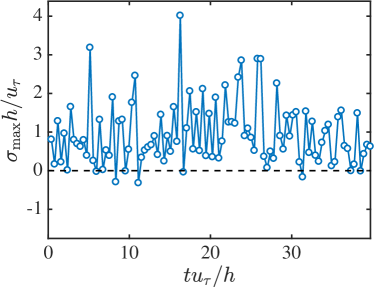
(a)

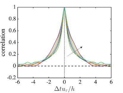
(b)

Figure 1: (a) The evolution of the maximum growth rate of the mean cross-flow $U(y,z,t)$. (b) The auto-correlation of the cross-flow $\langle U(y,z,t)\rangle_{z}$. The different lines are for $y/h=0.01,0.04,0.10,0.22,0.45,0.80$. The arrow indicates increasing $y/h$.

3 Experiments for discerning energy transfer mechanisms and preliminary results

3.1 Primary energy injection by modal instability

The effect of modal instability is assessed by freezing in time the mean cross-flow for case CH180 at time $t_{0}$ when $U(y,z,t)$ is modally unstable. At each time step, $f_{1}$ is computed such that $U(y,z,t)=U(y,z,t_{0})$ with $f_{2}=f_{3}=0$. Additionally, $\langle u\rangle_{xzt}$ is set to the same value as in case CH180. The lack of time evolution in $U$ eliminates the ability of energy extraction through parametric instability. The cross-flow can still support transient growth, but the algebraic growth of perturbations is expected to be overcome by the faster exponential growth provided by the modal instability of $U$. A total number of 100 uncorrelated flow fields with modally unstable $U(y,z,t_{0})$ were selected to run simulations. Note that as the base flow is frozen in time, the assumption of constant $U$ invoked for the stability analysis is rigorously satisfied. As an example, Figure 3 shows the instantaneous velocity field for one case after transients.

The resulting root-mean-squared (rms) fluctuating velocities for the statistical steady state are shown in Figure 3(a), together with those from CH180. Unsurprisingly, turbulent channel flows with persistent modally unstable mean cross-flow are capable of sustaining turbulence. The new flow reaches statistical equilibrium at a higher level of turbulence intensities owing to the additional mean tangential stress introduced by $f_{1}$, but the trends observed in Figure 3(a) are consistent with CH180 in terms of relative magnitude and wall-normal behavior. The transition to the new steady state is evidenced by Figure 3(b), which shows the time evolution of a selection of streamwise Fourier components before and after freezing the mean cross-flow. The adaptation time of turbulence upon imposition of constant $U$ is roughly $h/u_{\tau}$, consistent with the lifespan of large eddies in the flow (Lozano-Durán & Jiménez, 2014).

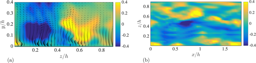
Figure 2: Experiment with fixed, unstable $U$: (a) Instantaneous velocity field in a $z-y$ plane at $x=0h$. (b) Instantaneous streamwise velocity in a $x-z$ plane at $y=0.1h$. Colors represent streamwise velocity and arrows are cross-flow velocities. Velocities are scaled in wall units of the baseline case.

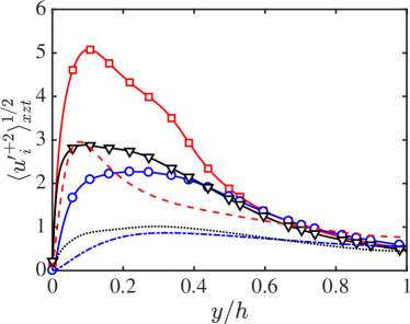
(a)

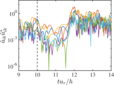
(b)

Figure 3: Experiment with fixed, unstable $U$: (a) Root-mean-squared fluctuating velocities for case CH180 (lines) and channel with frozen-in-time modally unstable mean cross-flow (symbols). Lines and symbols are: dashed and squares, streamwise; dash-dotted and circles, wall-normal; dotted and triangles, spanwise velocity fluctuations. (b) Time evolution of the energy associated with streamwise Fourier modes, $\hat{u}_{ik}\hat{u}^{*}_{ik}$, for $i=1,2,3$ and $k=0,1,2$ at $y=0.1h$, where $*$ denotes complex conjugation. The mean cross-flow is frozen at $tu_{\tau}/h=10$ (dashed black line).

The results reported above correspond to one particular $U(y,z,t_{0})$, but the conclusions are found to be robust for all mean cross-flows examined. Finally, it is important to highlight that while maintaining mean cross-flow in a modally unstable state does lead to sustained turbulence, whether this new state is similar in nature to unforced wall turbulence is an important question that is not investigated here and should be carefully addressed in future studies.

3.2 Energy injection by transient growth

The effect of non-modal transient growth as a main cause for energy injection is assessed by following a similar approach to that in Section 3.1. In this case, the cross-flow $U$ from CH180 is frozen at the instant $t_{0}$, when the flow is modally stable. The mean flow $\langle u\rangle_{xzt}$ is set to the same value as in case CH180. The set-up disposes of energy transfers that are due to both modal and parametric instabilities, while maintaining the transient growth of perturbations. The expected scenario consistent with sustained turbulence (e.g., Schoppa & Hussain, 2002) is the non-modal amplification of perturbations until saturation followed by nonlinear scattering and generation of new disturbances. However, plain visual inspection of the velocity field in Figure 5 reveals that this is not the case, and turbulence is distinctly lessened.

The rms fluctuating velocities for one experiment are shown in Figure 5(a). Turbulence reaches a quasi-laminar state with residual cross-flow turbulence intensities and non-negligible streamwise fluctuations required to support the prescribed $U(y,z,t_{0})$. The exponential decay of Fourier modes after freezing the mean cross-flow is clearly seen in Figure 5(b). The simulation was repeated for 20 different modally stable mean cross-flows $U(y,z,t_{0})$ and all cases decayed similarly to the example discussed above.

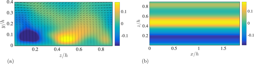
Figure 4: Experiment with fixed, stable $U$: (a) Instantaneous velocity field in a $z-y$ plane at $x=0h$. (b) Instantaneous streamwise velocity in a $x-z$ plane at $y=0.1h$. Colors represent streamwise velocity and arrows are cross-flow velocities. Velocities are scaled in wall units of the baseline case. Arrows in panel (a) are amplified by a factor of 10.

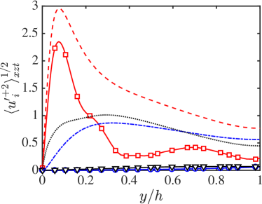
(a)

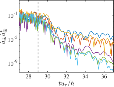
(b)

Figure 5: Experiment with fixed, stable $U$: (a) Root-mean-squared fluctuating velocities for case CH180 (lines) and channel with frozen-in-time modally stable mean cross-flow (symbols). Lines and symbols are: dashed and squares, streamwise; dash-dotted and circles, wall-normal; dotted and triangles, spanwise velocity fluctuations. (b) Time evolution of the energy associated to streamwise Fourier modes, $\hat{u}_{ik}\hat{u}^{*}_{ik}$, for $i=1,2,3$ and $k=0,1,2$ at $y=0.1h$, where $*$ denotes complex conjugate. The mean cross-flow is frozen in time at $tu_{\tau}/h=29$ (dashed black line).

3.3 Energy injection by transient growth with parametric instability

The maintenance of turbulence exclusively by transient growth with parametric instability is analyzed by a time-dependent mean cross-flow that is altered to be free of modal instabilities. To that end, we introduce the linear damping $f_{1}=-\mu(U-\langle u\rangle_{xz})$, $f_{2}=f_{3}=0$, where the parameter $\mu$ is a coefficient to be determined such that $U$ is modally stable for all times. The goal is to investigate the existence of self-sustained wall turbulence without any energy extraction from the mean cross-flow via modal instabilities.

Ideally, if $\partial\boldsymbol{u}^{\prime}\big{/}\partial t=A(\mu)\boldsymbol{u}^{\prime}$ is the linear equation governing the fluctuating velocities, the drag coefficient $\mu$ should be adjusted at each time step to bring the most unstable eigenvalue of $A$ to neutrality. In the present preliminary version of the work, we adopted a simplified approach where the value of $\mu$ is set constant in time. Then, a campaign of channel flow simulations driven by a constant streamwise mass flux was performed for values of $\mu$ ranging from $0$ up to $\mu_{c}\approx 1.3u_{\tau}/h$, above which the flow laminarizes.

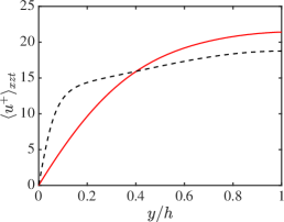
(a)

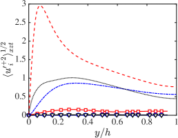
(b)

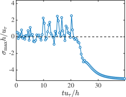
(c)

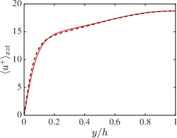
(d)

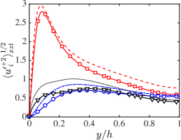
(e)

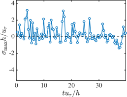
(f)

Figure 6: Experiment with linear drag on $U$: (a,d) Mean velocity profile for case CH180 (black dashed line) and channel with linear damping $-\mu(U-\langle u\rangle_{xz})$ (solid red line). (b,e) Root-mean-squared fluctuating velocities for case CH180 (lines) and channel with $-\mu(U-\langle u\rangle_{xz})$ (symbols). Lines and symbols are: dashed and squares, streamwise; dashed-dotted and circles, wall-normal; dotted and triangles, spanwise velocity fluctuations. (c,g) Time evolution of the maximum growth rate of $A$ for channel flow with linear damping $-\mu(U-\langle u\rangle_{xz})$. (a,b,c) are for $\mu=1.4u_{\tau}/h>\mu_{c}$ and (d,e,f) are for $\mu=1.2u_{\tau}/h<\mu_{c}$.

The mean and rms velocity profiles for $\mu=1.4u_{\tau}/h>\mu_{c}$ are shown in Figures 6(a,b). The flow is laminar with zero velocity fluctuations. Figure 6(c) shows the time history of the most unstable growth rate of $A$, which is constant and negative after transients. Figures 6(d,e,f) are equivalent to Figures 6(a,b,c) but for $\mu=1.2u_{\tau}/h<\mu_{c}$, which is the maximum value of $\mu$ that allows for sustained turbulence in a statistical steady state. The rms velocities are weaker with respect to case CH180, but they still resemble qualitatively those encountered in real turbulence. Although not shown, the de-correlation times for $U$ are similar to those for case CH180. Figure 6(f) shows that $U(z,y,t)$ is modally unstable $\sim$60% of the time based on $\sigma_{\mathrm{max}}>u_{\tau}/h/4$. The percentage is below the value obtained for case CH180 ($\sim$80%), which suggests that not all the modal instabilities are necessary to maintain turbulence with realistic one-point statistics.

Finally, a different numerical experiment is performed by including a linear damping into the equation for the fluctuating velocities, i.e., $f_{i}=-\mu^{\prime}u_{i}^{\prime}$, $i=1,2,3$. In this new set-up, we directly target the eigenvalues of $A$, whose real parts are reduced exactly by $\mu^{\prime}$ compared to the eigenvalues of $A$ for CH180. The maximum value of $\mu^{\prime}$ that allows for sustained turbulence is found to be $\mu^{\prime}_{c}\approx 1u_{\tau}/h$. The resulting flow statistics for $\mu^{\prime}$ that is marginally above and marginally below $\mu^{\prime}_{c}$ (Figure 7) yield similar conclusions as those reported above: turbulence only survives when $A$ is modally unstable (based on $\sigma_{\mathrm{max}}>u_{\tau}/h/4$) for a substantial fraction of the time simulated, in this case for $\sim$50% of the time when $\mu^{\prime}=0.9h/u_{\tau}<\mu^{\prime}_{c}$.

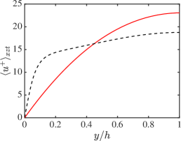
(a)

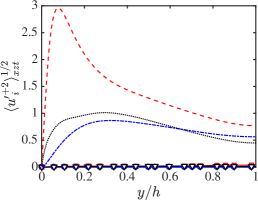
(b)

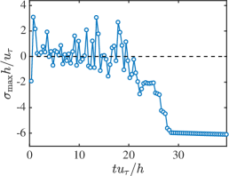
(c)

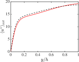
(d)

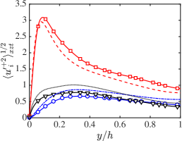
(e)

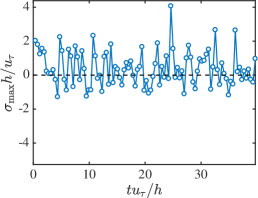
(f)

Figure 7: Experiment with linear drag on $\boldsymbol{u}^{\prime}$: (a,d) Mean velocity profile for case CH180 (black dashed line) and channel with linear damping $-\mu^{\prime}u^{\prime}_{i}$ (solid red line). (b,e) Root-mean-squared fluctuating velocities for case CH180 (dashed lines) and channel with $-\mu^{\prime}u^{\prime}_{i}$ (symbols). Lines and symbols are: dashed and squares, streamwise; dashed-dotted and circles, wall-normal; dotted and triangles, spanwise velocity fluctuations. (c,g) Time evolution of the maximum growth rate of $A$ for channel flow with linear damping $-\mu^{\prime}u^{\prime}_{i}$. (a,b,c) are for $\mu^{\prime}=1.1u_{\tau}/h>\mu_{c}^{\prime}$ and (d,e,f) are for $\mu^{\prime}=0.9u_{\tau}/h<\mu_{c}^{\prime}$.

4 Conclusions

We have studied the mechanism of energy injection from the mean flow to the fluctuating velocity necessary to maintain wall turbulence. This process is believed to be correctly represented by the linearized Navier–Stokes equations, and three potential linear mechanisms have been considered, namely, modal instability of the streamwise mean cross-flow $U(y,z,t)$, non-modal transient growth, and non-modal transient growth supported by parametric instability.

We have designed three numerical experiments of plane turbulent channel flow with additional forcing terms aiming to neutralize one or various linear mechanisms for energy extraction. To assess the effect of modal instabilities and non-modal transient growth of $U(y,z,t)$, we have computed turbulent channel flows with prescribed modally stable/unstable mean cross-flows frozen in time. In addition, transient growth with parametric instability was evaluated by adding a linear damping to the momentum equation of the mean cross-flow or to the fluctuation equations. This additional linear damping was chosen accordingly to render any modal instabilities stable and thus preclude energy transfer to the fluctuations from modal instabilities.

From our preliminary experiments, only cases with mean cross-flows capable of supporting modal instabilities were found to sustain turbulence. However, the question whether such a new turbulence complies with the same physical mechanisms as those occurring in actual (unforced) turbulence remains unanswered. On the other hand, cases exclusively supported by transient growth decayed until laminarization. For this preliminary study, this outcome should not be taken as a demonstration that transient growth alone aided or not by parametric instability is unable to maintain turbulence in actual flows, but just as an indication that we could not find a self-sustained turbulent system without the contribution of modal instabilities.

Future work will be devoted to the careful design of modified turbulent channel flows providing clear causal inference and quantification of the energy injection mechanisms in wall turbulence. Moreover, if indeed modal instability (or other) is the dominant mechanism responsible for transferring energy from the mean flow to the fluctuations, it should be detectable from unforced wall-turbulence simulation (e.g., CH180), and additional efforts will be carried on to analyze DNS data using non-intrusive techniques.

Appendix: Stability analysis

This appendix describes the linear stability analysis of a base mean cross-flow, which is inhomogeneous in two spatial directions. We assume the following velocity field

$${\mbox{\boldmath$u$}}=\left(U(y,z),0,0\right)+\varepsilon{\mbox{\boldmath$u$}}_{d},$$ (A 1)

where the base flow $U$ is assumed parallel, steady, and streamwise independent, and ${\mbox{\boldmath$u$}}_{d}$ is the disturbance. Substituting the velocity field into the incompressible Navier–Stokes equations and neglecting the nonlinear terms, we obtain

$$\frac{\partial u_{d}}{\partial x}+\frac{\partial v_{d}}{\partial y}+\frac{\partial w_{d}}{\partial z} =0,$$ (A 2a)

$$\frac{\partial u_{d}}{\partial t}+U\frac{\partial u_{d}}{\partial x}+v_{d}\frac{\partial U}{\partial y}+w_{d}\frac{\partial U}{\partial z} =-\frac{\partial p_{d}}{\partial x}+\nu\nabla^{2}u_{d},$$ (A 2b)

$$\frac{\partial v_{d}}{\partial t}+U\frac{\partial v_{d}}{\partial x} =-\frac{\partial p_{d}}{\partial y}+\nu\nabla^{2}v_{d},$$ (A 2c)

$$\frac{\partial w_{d}}{\partial t}+U\frac{\partial w_{d}}{\partial x} =-\frac{\partial p_{d}}{\partial z}+\nu\nabla^{2}w_{d},$$ (A 2d)

where $p_{d}$ is the disturbance pressure. The boundary conditions are no slip and impermeability on the channel walls. In the current study, the stability analysis has been performed only on a half-channel. Therefore, no slip and impermeability were imposed on the channel center, as we are interested only in the instabilities close to the wall.

The base flow is periodic along the spanwise direction, and it is often useful to describe it in terms of a truncated Fourier expansion. In such cases, a Floquet analysis is performed with respect to the span (see, e.g., Karp & Cohen, 2014). Nevertheless, for an arbitrary base flow, such as the one considered here, it is not beneficial to invoke Floquet theory. Therefore, we assume the following form for the disturbance,

$${\mbox{\boldmath$q$}}_{d}=\hat{{\mbox{\boldmath$q$}}}_{d}(y,z)e^{\lambda t+i\alpha x},$$ (A 3)

where ${\mbox{\boldmath$q$}}_{d}=(u_{d},v_{d},w_{d},p_{d})^{\mathsf{T}}$, $\alpha$ is the streamwise wavenumber, and $\lambda$ is the temporal complex eigenvalue. The eigenvalue can be written as $\lambda=\sigma+i\omega$, where $\sigma$ is the growth rate and $\omega$ is the frequency. The linearized equations above are discretized along both inhomogeneous directions using spectral methods. Along the wall-normal direction, a Chebyshev grid is used for $y\in[0,h]$, and along the spanwise direction a Fourier grid is used for $z\in[0,L_{z}]$.

Substituting the disturbance into the linearized equations, they can be rearranged as a generalized eigenvalue problem for the calculation of $\lambda$,

$$\begin{pmatrix}\mathsfbi{D_{x}}~{}&\mathsfbi{D_{y}}~{}&\mathsfbi{D_{z}}~{}&\mathsfbi{O}\\ \mathsfbi{C}~{}&\mathsfbi{U_{y}}~{}&\mathsfbi{U_{z}}~{}&\mathsfbi{D_{x}}\\ \mathsfbi{O}~{}&\mathsfbi{C}~{}&\mathsfbi{O}~{}&\mathsfbi{D_{y}}\\ \mathsfbi{O}~{}&\mathsfbi{O}~{}&\mathsfbi{C}~{}&\mathsfbi{D_{z}}\end{pmatrix}\begin{pmatrix}\begin{array}[]{c}\tilde{u}_{d}\\ \tilde{v}_{d}\\ \tilde{w}_{d}\\ \tilde{p}_{d}\end{array}\end{pmatrix}=\lambda\begin{pmatrix}\mathsfbi{O}~{}&\mathsfbi{O}~{}&\mathsfbi{O}~{}&\mathsfbi{O}\\ -\mathsfbi{I}~{}&\mathsfbi{O}~{}&\mathsfbi{O}~{}&\mathsfbi{O}\\ \mathsfbi{O}~{}&-\mathsfbi{I}~{}&\mathsfbi{O}~{}&\mathsfbi{O}\\ \mathsfbi{O}~{}&\mathsfbi{O}~{}&-\mathsfbi{I}~{}&\mathsfbi{O}\end{pmatrix}\begin{pmatrix}\tilde{u}_{d}\\ \tilde{v}_{d}\\ \tilde{w}_{d}\\ \tilde{p}_{d}\end{pmatrix}.$$ (A 4)

Here, $\mathsfbi{I}$ is the identity matrix, $\mathsfbi{O}$ is a zero matrix, $\tilde{u}_{d}$ (and similarly $\tilde{v}_{d},\tilde{w}_{d},\tilde{p}_{d}$) is a one-dimensional representation of a two-dimensional vector

$$\tilde{u}_{d}=\big{(}\hat{u}_{d}(y,z_{1}),\hat{u}_{d}(y,z_{2}),\dots,\hat{u}_{d}(y,z_{N_{z}})\big{)}^{\mathsf{T}},$$ (A 5)

and the matrices $\mathsfbi{C}$, $\mathsfbi{U_{y}}$, $\mathsfbi{U_{z}}$, $\mathsfbi{D_{x}}$, $\mathsfbi{D_{y}}$, and $\mathsfbi{D_{z}}$ are given by

$$\mathsfbi{C} =i\alpha\;\textnormal{diag}\left(\mathsfbi{U}\right)-\nu\left(\mathsfbi{\bar{I}_{z}}\otimes\mathsfbi{\bar{D}^{2}_{y}}+\mathsfbi{\bar{D}^{2}_{z}}\otimes\mathsfbi{\bar{I}_{y}}-\alpha^{2}\mathsfbi{\bar{I}_{z}}\otimes\mathsfbi{\bar{I}_{y}}\right),$$ (A 6a)

$$\mathsfbi{U_{y}} =\textnormal{diag}\left\{\left(\mathsfbi{\bar{I}_{z}}\otimes\mathsfbi{\bar{D}_{y}}\right)\mathsfbi{U}\right\},$$ (A 6b)

$$\mathsfbi{U_{z}} =\textnormal{diag}\left\{\left(\mathsfbi{\bar{D}_{z}}\otimes\mathsfbi{\bar{I}_{y}}\right)\mathsfbi{U}\right\},$$ (A 6c)

$$\mathsfbi{D_{x}} =i\alpha\;\mathsfbi{\bar{I}_{z}}\otimes\mathsfbi{\bar{I}_{y}},$$ (A 6d)

$$\mathsfbi{D_{y}} =\mathsfbi{\bar{I}_{z}}\otimes\mathsfbi{\bar{D}_{y}},$$ (A 6e)

$$\mathsfbi{D_{z}} =\mathsfbi{\bar{D}_{z}}\otimes\mathsfbi{\bar{I}_{y}},$$ (A 6f)

where $\otimes$ is the Kronecker product and $\mathsfbi{U}$ is a one-dimensional representation of $U$ (similarly to $\tilde{u}_{d}$). The matrices $\mathsfbi{\bar{I}_{y}}$ and $\mathsfbi{\bar{I}_{z}}$ are identity matrices of dimensions $N_{y}\times N_{y}$ and $N_{z}\times N_{z}$, respectively, and $\mathsfbi{\bar{D}_{y}}$ and $\mathsfbi{\bar{D}_{z}}$ are matrices that represent derivation with respect to the $y$ and $z$ coordinates, respectively. The eigenvalue problem is solved numerically using the software Matlab, with $N_{y}=101$ and $N_{z}=32$. All the calculations were conducted for $\alpha=2\pi/L_{x}$.

References

- Adrian (2007) Adrian, R. J. 2007 Hairpin vortex organization in wall turbulence. Phys. Fluids 19, 041301.
- del Álamo & Jiménez (2006) del Álamo, J. C. & Jiménez, J. 2006 Linear energy amplification in turbulent channels. J. Fluid Mech. 559, 205–213.
- Bae et al. (2018a) Bae, H. J., Lozano-Durán, A., Bose, S. T. & Moin, P. 2018a Dynamic slip wall model for large-eddy simulation. J. Fluid Mech. 859, 400–432.
- Bae et al. (2018b) Bae, H. J., Lozano-Durán, A., Bose, S. T. & Moin, P. 2018b Turbulence intensities in large-eddy simulation of wall-bounded flows. Phys. Rev. Fluids 3, 014610.
- Butler & Farrell (1992) Butler, K. M. & Farrell, B. F. 1992 Optimal perturbations and streak spacing in wall-bounded turbulent shear flow. Phys. Fluids A 5, 774.
- Chernyshenko & Baig (2005) Chernyshenko, S. I. & Baig, M. F. 2005 The mechanism of streak formation in near-wall turbulence. J. Fluid Mech. 544, 99–131.
- Farrell & Ioannou (1998) Farrell, B. F. & Ioannou, P. J. 1998 Perturbation structure and spectra in turbulent channel flow. Theor. Comput. Fluid Dyn. 11, 215–227.
- Farrell & Ioannou (2012) Farrell, B. F. & Ioannou, P. J. 2012 Dynamics of streamwise rolls and streaks in turbulent wall-bounded shear flow. J. Fluid Mech. 708, 149–196.
- Farrell & Ioannou (2017) Farrell, B. F. & Ioannou, P. J. 2017 Statistical state dynamics-based analysis of the physical mechanisms sustaining and regulating turbulence in Couette flow. Phys. Rev. Fluids 2, 084608.
- Farrell et al. (2016) Farrell, B. F., Ioannou, P. J., Jiménez, J., Constantinou, N. C., Lozano-Durán, A. & Nikolaidis, M.-A. 2016 A statistical state dynamics-based study of the structure and mechanism of large-scale motions in plane Poiseuille flow. J. Fluid Mech. 809, 290–315.
- Hack & Moin (2018) Hack, M. J. P. & Moin, P. 2018 Coherent instability in wall-bounded shear. J. Fluid Mech. 844, 917–955.
- Hamilton et al. (1995) Hamilton, J. M., Kim, J. & Waleffe, F. 1995 Regeneration mechanisms of near-wall turbulence structures. J. Fluid Mech. 287, 317–348.
- Högberg et al. (2003) Högberg, M., Bewley, T. R. & Henningson, D. S. 2003 Linear feedback control and estimation of transition in plane channel flow. J. Fluid Mech. 481, 149–175.
- Hwang & Cossu (2010) Hwang, Y. & Cossu, C. 2010 Linear non-normal energy amplification of harmonic and stochastic forcing in the turbulent channel flow. J. Fluid Mech. 664, 51–73.
- Jiménez (2012) Jiménez, J. 2012 Cascades in wall-bounded turbulence. Annu. Rev. Fluid Mech. 44, 27–45.
- Jiménez (2013) Jiménez, J. 2013 How linear is wall-bounded turbulence? Phys. Fluids 25, 110814.
- Jiménez (2018) Jiménez, J. 2018 Coherent structures in wall-bounded turbulence. J. Fluid Mech. 842, P1.
- Jiménez & Moin (1991) Jiménez, J. & Moin, P. 1991 The minimal flow unit in near-wall turbulence. J. Fluid Mech. 225, 213–240.
- Karp & Cohen (2014) Karp, M. & Cohen, J. 2014 Tracking stages of transition in Couette flow analytically. J. Fluid Mech. 748, 896–931.
- Kawahara et al. (2003) Kawahara, G., Jiménez, J., Uhlmann, M. & Pinelli, A. 2003 Linear instability of a corrugated vortex sheet – a model for streak instability. J. Fluid Mech. 483, 315–342.
- Kim et al. (1971) Kim, H. T., Kline, S. J. & Reynolds, W. C. 1971 The production of turbulence near a smooth wall in a turbulent boundary layer. J. Fluid Mech. 50, 133–160.
- Kim & Lim (2000) Kim, J. & Lim, J. 2000 A linear process in wall bounded turbulent shear flows. Phys. Fluids 12, 1885–1888.
- Kim & Moin (1985) Kim, J. & Moin, P. 1985 Application of a fractional-step method to incompressible Navier-Stokes equations. J. Comp. Phys. 59, 308–323.
- Klebanoff et al. (1962) Klebanoff, P. S., Tidstrom, K. D. & Sargent, L. M. 1962 The three-dimensional nature of boundary-layer instability. J. Fluid Mech. 12, 1–34.
- Kline et al. (1967) Kline, S. J., Reynolds, W. C., Schraub, F. A. & Runstadler, P. W. 1967 The structure of turbulent boundary layers. J. Fluid Mech. 30, 741–773.
- Landahl (1975) Landahl, M. T. 1975 Wave breakdown and turbulence. SIAM J. Appl. Math 28, 735–756.
- Lozano-Durán & Bae (2016) Lozano-Durán, A. & Bae, H. J. 2016 Turbulent channel with slip boundaries as a benchmark for subgrid-scale models in LES. Annual Research Briefs, Center for Turbulence Research, pp. 97–103.
- Lozano-Durán et al. (2018) Lozano-Durán, A., Hack, M. J. P. & Moin, P. 2018 Modeling boundary-layer transition in direct and large-eddy simulations using parabolized stability equations. Phys. Rev. Fluids 3, 023901.
- Lozano-Durán & Jiménez (2014) Lozano-Durán, A. & Jiménez, J. 2014 Time-resolved evolution of coherent structures in turbulent channels: characterization of eddies and cascades. J. Fluid Mech. 759, 432–471.
- Mansour et al. (1988) Mansour, N. N., Kim, J. & Moin, P. 1988 Reynolds-stress and dissipation-rate budgets in a turbulent channel flow. J. Fluid Mech. 194, 15–44.
- Orlandi (2000) Orlandi, P. 2000 Fluid Flow Phenomena: A Numerical Toolkit. Springer.
- Panton (2001) Panton, R. L. 2001 Overview of the self-sustaining mechanisms of wall turbulence. Prog. Aerosp. Sci. 37, 341–383.
- Schmid (2007) Schmid, P. J. 2007 Nonmodal stability theory. Annu. Rev. Fluid Mech. 39, 129–162.
- Schoppa & Hussain (2002) Schoppa, W. & Hussain, F. 2002 Coherent structure generation in near-wall turbulence. J. Fluid Mech. 453, 57–108.
- Smits et al. (2011) Smits, A. J., McKeon, B. J. & Marusic, I. 2011 High-Reynolds number wall turbulence. Annu. Rev. Fluid Mech. 43, 353–375.
- Vaughan & Zaki (2011) Vaughan, N. J. & Zaki, T. A. 2011 Stability of zero-pressure-gradient boundary layer distorted by unsteady Klebanoff streaks. J. Fluid Mech. 681, 116–153.
- Waleffe (1997) Waleffe, F. 1997 On a self-sustaining process in shear flows. Phys. Fluids 9, 883–900.
- Wray (1990) Wray, A. A. 1990 Minimal-storage time advancement schemes for spectral methods. Tech. Rep. MS 202 A-1. NASA Ames Research Center.