Emergent hydrodynamics in non-equilibrium quantum systems

Abstract

A tremendous amount of recent attention has focused on characterizing the dynamical properties of periodically driven many-body systems. Here, we use a novel numerical tool termed ‘density matrix truncation’ (DMT) to investigate the late-time dynamics of large-scale Floquet systems. We find that DMT accurately captures two essential pieces of Floquet physics, namely, prethermalization and late-time heating to infinite temperature. Moreover, by implementing a spatially inhomogeneous drive, we demonstrate that an interplay between Floquet heating and diffusive transport is crucial to understanding the system’s dynamics. Finally, we show that DMT also provides a powerful method for quantitatively capturing the emergence of hydrodynamics in static (un-driven) Hamiltonians; in particular, by simulating the dynamics of generic, large-scale quantum spin chains (up to $L=100$), we are able to directly extract the energy diffusion coefficient.

Understanding the non-equilibrium dynamics of strongly correlated quantum systems represents a central challenge at the interface of condensed matter, atomic physics and quantum information science. This challenge stems in part from the fact that such systems can be taken out of equilibrium in a multitude of different ways, each with its own set of expectations and guiding intuition.

For example, under a quench, one typically expects a many-body system to quickly evolve toward local thermal equilibrium Deutsch (1991); Srednicki (1994); Rigol et al. (2008); D’Alessio et al. (2016); Calabrese et al. ; Gogolin and Eisert (2016). At first sight, this suggests a simple description. However, capturing both the microscopic details of short-time thermalization as well as the cross-over to late-time hydrodynamics remains an open challenge Potter et al. (2015); Vosk et al. (2015); Agarwal et al. (2015); Žnidarič et al. (2016); Luitz et al. (2016); Khait et al. (2016); Luitz and Bar Lev (2016); Sahu et al. (2018); Bohrdt et al. (2017). Indeed, despite nearly a century of progress, no general framework exists for perhaps the simplest question: How does one derive a classical diffusion coefficient from a quantum many-body Hamiltonian?

Alternatively, a many-body system can also be taken out of equilibrium via periodic (Floquet) driving — a strategy which has received a tremendous amount of recent attention in the context of novel Floquet phases of matter Else et al. (2016); Khemani et al. (2016); von Keyserlingk and Sondhi (2016a, b); von Keyserlingk et al. (2016); Lindner et al. (2011); Kitagawa et al. (2010); Yao et al. (2017); Choi et al. (2017); Zhang et al. (2017). In this case, the non-equilibrium system is generically expected to absorb energy from the driving field (so-called Floquet heating) until it approaches a featureless infinite temperature state Prosen (1998, 1999); Lazarides et al. (2014); D’Alessio and Rigol (2014); Bukov et al. (2015a); Machado et al. (2019).

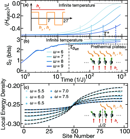
Figure 1: Floquet thermalization of an $L=100$ spin chain. (a) Average energy density measured with respect to $H_{\text{static}}\approx D_{\mathrm{eff}}$ under a global drive. The heating timescale $\tau^{*}$ is extracted from the energy’s exponential approach to its infinite-temperature value, and depends exponentially on the driving frequency (for explicit scaling, see Fig. 4a.) (b) The second Rényi entropy of the leftmost three sites. The dashed lines are computed using the prethermal Gibbs ensemble SM . (c) Spatial profiles of energy density under a half-system drive with $\langle H_{\text{static}}\rangle/L=-0.25$. Insets: the drive’s time dependence (a) and schematics of the global drive (b) and the half-system drive (c).

While these questions are naturally unified under the umbrella of non-equilibrium dynamics fn (1), understanding the interplay between Floquet heating, emergent hydrodynamics and microscopic thermalization represents a crucial step toward the characterization and control of non-equilibrium many-body systems Abanin et al. (2015); Mori et al. (2016); Abanin et al. (2017a); Kuwahara et al. (2016); Abanin et al. (2017b); Else et al. (2017); Bukov et al. (2015b); Weidinger and Knap (2017). That one expects such connections can already been seen in certain limits; for example, in the limit of a high-frequency Floquet drive, energy absorption is set by an extremely slow heating rate. Thus, one anticipates a relatively long timescale where the system’s stroboscopic dynamics can be captured by an effective static prethermal Hamiltonian. These expectations immediately lead to the following question: How do the late-time dynamics of driven quantum systems account for both the prethermal Hamiltonian’s hydrodynamics and the energy absorption associated with Floquet heating?

Until now, such questions have remained largely unexplored owing to the fact that they sit in a region of phase space where neither theoretical techniques nor numerical methods easily apply. However, a number of recently proposed numerical methods White et al. (2018); Leviatan et al. ; Wurtz et al. (2018); Wurtz and Polkovnikov ; Zaletel and Pollmann promise to bridge this gap and directly connect microscopic models to emergent macroscopic hydrodynamics. Here, we will focus on one such method — density matrix truncation (DMT) White et al. (2018) — which modifies time-evolving block decimation (TEBD) by representing states as matrix product density operators (MPDOs) and prioritizing short-range (over long-range) correlations.

Working with a generic, one-dimensional spin model, in this Letter, we use DMT to investigate a broad range of non-equilibrium phenomena ranging from Floquet heating to emergent hydrodynamics. Our main results are three fold. First, we find that DMT accurately captures two essential pieces of Floquet physics: prethermalization and heating to infinite temperature (Fig. 1). Crucially, the truncation step intrinsic to DMT enables us to efficiently explore the late-time dynamics of large-scale quantum systems (up to $L=100$), at the cost of imperfectly simulating the system’s early-time dynamics.

This trade-off hinges on DMT’s efficient representation of local thermal states, making it a natural tool for studying emergent hydrodynamics. Our latter two results illustrate this in two distinct contexts: 1) directly measuring the energy diffusion coefficient for a static Hamiltonian, and 2) demonstrating the interplay between Floquet heating and diffusion in an inhomogeneously driven spin chain. We hasten to emphasize that such calculations are fundamentally impossible for either exact diagonalization based methods (owing to the size of the Hilbert space) or conventional TEBD methods (owing to the large amount of entanglement at late times).

Model and phenomenology—We study the dynamics of a one-dimensional spin-$1/2$ chain whose evolution is governed by a time periodic Hamiltonian $H(t)=H_{\text{static}}+H_{\mathrm{drive}}(t)$, where

$$\begin{split}H_{\text{static}}&=\sum^{L-1}_{i=1}[J\sigma^{z}_{i}\sigma^{z}_{i+1}+J_{x}\sigma^{x}_{i}\sigma^{x}_{i+1}]+h_{x}\sum_{i=1}^{L}\sigma^{x}_{i}~{},\end{split}$$ (1)

with $\sigma^{\alpha}_{i}$ being the Pauli operators acting on site $i$ fn (2). The drive, $H_{\mathrm{drive}}(t)=H_{\mathrm{drive}}(t+T)$, exhibits a period $T=2\pi/\omega$ and corresponds to an oscillating field in the $\hat{y}$ and $\hat{z}$ directions:

$$H_{\mathrm{drive}}(t)=\sum_{i=1}^{L}v_{i}(t)~{}(h_{y}\sigma^{y}_{i}+h_{z}\sigma^{z}_{i})~{}.$$ (2)

In this work we will consider two different driving protocols (Fig. 1 insets) a global drive, with all spins driven [$v_{i}(t)=\operatorname{sgn}\cos(\omega t)$], and a half-system drive, with only the right half driven [$v_{i\leq L/2}(t)=0$ and $v_{i>L/2}(t)=\operatorname{sgn}\cos(\omega t)$]. Throughout the letter, we work in the high-frequency regime with $\omega\geq 5J$, and choose the parameters to be $\{J,J_{x},h_{x},h_{y},h_{z}\}=\{1,0.75,0.21,0.17,0.13\}$. We expect our choice of the model and parameters to be generic as we observe the same phenomenology upon varying both the parameters and the interaction Hamiltonian SM .

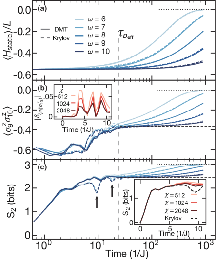
Figure 2: Comparison between DMT and Krylov of the time evolution of an $L=20$ spin chain under a global drive (at fixed bond dimension $\chi=64$). (a) Average energy density $\langle H_{\text{static}}\rangle/L$. (b) A typical local observable $\sigma^{z}_{9}\sigma^{z}_{10}$. (c) The second Rényi entropy $S_{2}$ of the leftmost three sites. The arrows mark resonance-like dips, which DMT fails to capture SM . The dashed lines are computed using the prethermal Gibbs ensemble. Insets (early-time behavior at frequency $\omega=10$): (b) errors in the local observable $\delta_{\langle\sigma^{z}_{9}\sigma^{z}_{10}\rangle}=\langle\sigma^{z}_{9}\sigma^{z}_{10}\rangle_{\mathrm{DMT}}-\langle\sigma^{z}_{9}\sigma^{z}_{10}\rangle_{\mathrm{Kry}}$, (c) errors in $S_{2}$.

The quenched dynamics of a high-frequency driven system is characterized by two timescales. The heating timescale, $\tau^{*}$ (Fig. 1a), determines the rate of energy absorption from the drive and is proven to be at least exponential in the frequency of the drive, $\tau^{*}\geq\mathcal{O}(e^{\omega/J_{\mathrm{local}}})$, where $J_{\text{local}}$ is a local energy scale  Abanin et al. (2015); Mori et al. (2016); Kuwahara et al. (2016); Abanin et al. (2017a, b); Else et al. (2017). Up until $\tau^{*}$, the stroboscopic dynamics of the system is well described by the static prethermal Hamiltonian $D_{\mathrm{eff}}=H_{\mathrm{static}}+\mathcal{O}(\omega^{-1})$, which can be obtained as the truncation of the Floquet-Magnus expansion of the evolution operator Kuwahara et al. (2016); Abanin et al. (2017a, b). The prethermalization timescale, $\tau_{D_{\mathrm{eff}}}$ (Fig. 1a,b), determines the time at which the system approaches an equilibrium state with respect to $D_{\mathrm{eff}}$. When $\tau_{D_{\mathrm{eff}}}\ll\tau^{*}$, the system exhibits a well defined, long-lived prethermal regime.

In Figs. 1a,b, we illustrate these two timescales by computing the dynamics of an $L=100$ Floquet spin chain using DMT fn (3). The average energy density $\langle H_{\text{static}}(t)\rangle/L$ exhibits the expected phenomenology (Fig. 1a): it remains constant (up to $\omega^{-1}$ corrections) until $\tau^{*}$, after which it begins to approach its infinite temperature value $\langle H_{\text{static}}\rangle_{T=\infty}=0$.

To probe the prethermalization timescale $\tau_{D_{\mathrm{eff}}}$, a different diagnostic is needed. In particular, we compute the second Rényi entropy, $S_{2}=-\log_{2}\operatorname{Tr}[\rho^{2}_{\mathrm{s}}]$, where $\rho_{\mathrm{s}}$ is the reduced density matrix of the three leftmost spins. While the system begins in a product state with $S_{2}=0$, its entropy quickly approaches a prethermal plateau, consistent with the Gibbs state of $D_{\mathrm{eff}}$ at a temperature that matches the initial energy density (Fig. 1b) SM . The timescale at which this occurs corresponds to $\tau_{D_{\mathrm{eff}}}$ and, indeed, we observe $\tau_{D_{\mathrm{eff}}}\sim 1/J_{\mathrm{local}}$ independent of the driving frequency $\omega$. Similar to the energy density, at late times $t>\tau^{*}$, $S_{2}$ begins to approach its infinite temperature value, $S_{2}^{T=\infty}=3$ bits.

Benchmarking DMT—To confirm the reliability of DMT in the simulation of Floquet dynamics, we compare it with Krylov subspace methods fn (8); Hernandez et al. (2005); Roman et al. (2016); Balay et al. (1997). This analysis not only gauges the applicability of DMT, but also leads to insights into the nature of the Floquet heating process.

Time evolution with DMT proceeds via two repeating steps: a TEBD-like approximation of the time evolution unitary and a truncation of the MPDO. In the TEBD-like step, we Trotter decompose the time evolution operator into a series of local gates which we then apply to the MPDO White et al. (2018). Because each local gate application increases the bond dimension of the corresponding tensors, we must truncate them back to a fixed maximum bond dimension, which we call $\chi$. During this truncation step, a conventional TEBD method will discard the terms which contribute the least to the entanglement Schollwöck (2005); Orús and Vidal (2008). As a result, this truncation is agnostic to the locality of the discarded correlations. By contrast, in DMT we explicitly prioritize the preservation of short-range correlations White et al. (2018). To this end, DMT separates $\chi$ into two contributions: $\chi=\chi^{\mathrm{preserve}}+\chi^{\mathrm{extra}}$. $\chi^{\mathrm{preserve}}=2^{\ell}$ is used to store the information of all observables on $\ell$ contiguous sites around the truncated tensor—we call $\ell$ the preservation diameter SM ; fn (4). $\chi^{\mathrm{extra}}$ is then used to preserve the remaining correlations with largest magnitude. Crucially, the preservation of short-range correlations allows DMT to conserve (up to Trotter errors) the instantaneous energy density White et al. (2018). To be more specific, in Floquet systems, DMT conserves $H(t)$ at each instant, but it does not explicitly conserve $D_{\mathrm{eff}}$.

We utilize three diagnostics to compare the time evolution between DMT and Krylov: the average energy density (Fig. 2a), local two-point correlation functions (Fig. 2b), and the second Rényi entropy (Fig. 2c).

At early times ($t<\tau_{D_{\mathrm{eff}}}$), one observes substantial disagreements between DMT and Krylov (Fig. 2b,c). This is to be expected. Indeed, the accurate description of early-time thermalization dynamics depends sensitively on the details of long-range correlations which DMT does not capture. An exception to this is the energy density, whose changes are expected to be exponentially small in frequency Abanin et al. (2015); Mori et al. (2016); Kuwahara et al. (2016); Abanin et al. (2017a). This is indeed born out by the numerics where one finds that $\langle H_{\mathrm{static}}\rangle/L$ remains quasi-conserved and in excellent agreement with Krylov (Fig. 2a).

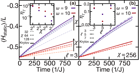
Figure 3: Energy density at (a) bond dimension $\chi=32,64,128$ and (b) the preservation diameter $\ell=3,5,7$. Insets: relative error in the heating rate $\eta_{\Gamma}=|\Gamma_{\mathrm{DMT}}-\Gamma_{\mathrm{Krylov}}|/\Gamma_{\mathrm{Krylov}}$, where $\Gamma=1/\tau^{*}_{E}$ is defined by $\frac{d}{dt}\langle H_{\text{static}}\rangle=-\Gamma\langle H_{\text{static}}\rangle.$

One might naively expect the early-time disagreements to lead to equally large intermediate-time ($\tau_{D_{\mathrm{eff}}}<t<\tau^{*}$) deviations. This is not what we observe. Indeed, all three diagnostics show excellent agreement between DMT and Krylov (Fig. 2). This arises from a confluence of two factors. First, as aforementioned, DMT accurately captures the system’s energy density, which in turn, fully determines the prethermal Gibbs state; second, DMT can efficiently represent such a Gibbs state. Thus, although DMT fails to capture the approach to the prethermal Gibbs state, it nevertheless reaches the same equilibrium state at $t\sim\tau_{D_{\mathrm{eff}}}$. Afterwards (for $t>\tau_{D_{\mathrm{eff}}}$), the system is simply evolving between different Gibbs states of $D_{\mathrm{eff}}$, wherein one expects agreement between DMT and Krylov even at relatively low bond dimension (Fig. 2).

Small disagreements between DMT and Krylov, however, re-emerge at very late times ($t>\tau^{*}$) and large frequencies, reflecting the physical nature of Floquet heating (Fig. 2a). In particular, as the frequency increases, absorbing an energy quantum from the drive requires the correlated rearrangement of a greater number of spins Abanin et al. (2015); Mori et al. (2016); Abanin et al. (2017a). However, these longer-ranged correlations are not strictly preserved by DMT, leading to an artificial (truncation-induced) suppression of heating at large frequencies (Fig. 3).

This raises the question: How does the accuracy of DMT converge with both bond dimension and preservation diameter? As expected, increasing $\chi$ at fixed $\ell$ improves the accuracy of DMT since the amount of information preserved during each truncation step is greater, Fig. 3a. Curiously, tuning $\ell$ at fixed $\chi$ can also affect the accuracy, despite not changing the amount of information preserved, Fig. 3b. This suggests the tantalizing possibility that one can achieve high accuracy at relatively low bond dimension by carefully choosing the operators which are preserved.

Floquet heating dynamics—As a first demonstration of DMT’s potential for extracting quantitative information about the Floquet dynamics, we directly measure the heating rate. We find that both $\langle H_{\text{static}}\rangle/L$ and $S_{2}$ exhibit an exponential approach toward their infinite-temperature values: $|\langle H_{\text{static}}\rangle/L|\propto e^{-t/\tau^{*}_{E}}$ and $(S_{2}^{T=\infty}-S_{2})\propto e^{-2t/\tau^{*}_{S}}$. To this end, we extract $\tau^{*}_{E}$ and $\tau^{*}_{S}$ as independent measures of the Floquet heating timescale SM . Crucially, they agree with one another across all system sizes studied ($L=20$–$100$), as shown in Fig. 4a. Varying the frequency of the drive further allows us to extract the effective local energy scale which controls the heating dynamics: $J_{\mathrm{local}}^{E}=1.21\pm 0.04$ and $J_{\text{local}}^{S}=1.16\pm 0.04$. This is consistent with the microscopic onsite energy scale, $\|H_{\text{static}}\|/L\simeq 1.26$ fn (5).

Observing emergent hydrodynamics—Having established that DMT accurately captures the late-time thermalization of Floquet systems, we now apply it to the study of a much broader question: the emergent hydrodynamics of large (undriven) quantum spin chains ($L=100$). In particular, our main goal here is to measure the diffusion coefficient as a function of temperature.

Our setup is the following. On top of an initial thermal state with respect to $H_{\text{static}}$, we add a small spatial inhomogeneity in the energy density (taken to be a Fourier mode) SM . As the system evolves under $H_{\text{static}}$, one finds that the amplitude of this spatial variation decays exponentially, with a rate that scales as $q^{2}$, where $q$ is the wave-vector of the Fourier mode. This quadratic scaling is characteristic of diffusion and confirms the emergence of hydrodynamics from our microscopic quantum Hamiltonian SM . By further varying the temperature of the initial Gibbs ensemble, one can also study the diffusion coefficient, $D(\epsilon)$, as a function of the energy density $\epsilon$ (Fig. 4b) fn (6).

We emphasize that such a numerical observation of emergent hydrodynamics is well beyond the reach of conventional numerics and fundamentally leverages DMT’s ability to prepare and evolve highly-entangled states near thermal equilibrium. Moreover, we note that our procedure can also be applied to the study of integrable systems, where different types of anomalous transport can occur Ljubotina et al. (2017); Bulchandani et al. (2018); Gopalakrishnan and Vasseur (2019); Castro-Alvaredo et al. (2016); Bertini et al. (2016); Misguich et al. (2017); Gobert et al. (2005). We highlight this by computing spin transport in the XXZ model and observing ballistic, super-diffusive and diffusive exponents as a function of the Ising anisotropy (for details see SM ).

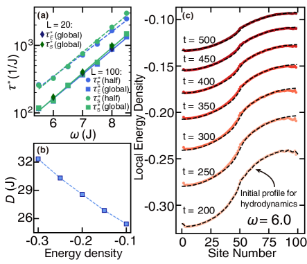
Figure 4: (a) Heating timescale, $\tau^{*}$, extracted in energy density ($E$) and subsystem entropy ($S_{2}$) for $L=20,100$. In agreement with theoretical prediction, $\tau^{*}$ depends exponentially on $\omega$. For both driving protocols, we extract the same local energy scale $J_{local}^{E}\approx 1.21$. However, the half-system drive exhibits a heating timescale twice as large as the global drive. (b) Energy dependence of the diffusion coefficient in the undriven spin chain. (c) Dynamics of the energy density with half-system drive. Solid curves are computed using DMT. Dashed black curves are computed using a hydrodynamical equation, Eq. 3, where one feeds in the DMT-calculated energy-density profile at time $t=200$. Subsequent time evolution under the differential equation quantitatively reproduces the exact results from DMT.

Interplay between driving and hydrodynamics—Taking things one step further, we now combine the two previous settings and explore a situation where the interplay between Floquet heating and diffusive transport is crucial for understanding the system’s thermalization dynamics. In particular, let us consider the time evolution of a spin chain where only the right half of the system is periodically driven (inset, Fig. 1c). At time $t=0$, the system is initialized in a Néel state with a domain wall every four spins fn (3).

After an initial period of local equilibration, the combination of inhomogenous driving and interactions leads to three distinct features in the dynamics of the local energy density, as illustrated in Fig. 4c. First, the local energy density on the right half of the spin chain is larger, reflecting the location where driving, and thus Floquet heating, is occurring. Second, the energy density across the entire chain gradually increases in time as energy from the right half is transported toward the left half. Third, as the system approaches its infinite temperature state, the overall energy-density inhomogeneity between the left and right halves of the system is reduced.

Leveraging our previous characterizations of both heating and transport, we combine them into such a single hydrodynamical description. The only missing element is a small correction to the transport due to the inhomogeneity of the drive, whose strength we characterize by a small, frequency dependent parameter $\eta$.

We now ask the following question: Can all three of these behaviors be quantitatively captured using a simple hydrodynamical equation? If so, one might naturally posit the following modified diffusion equation SM :

$$\partial_{t}\epsilon(x,t)=D(\epsilon)\partial^{2}_{x}\Big{(}[1+\eta g(x)]\epsilon(x,t)\Big{)}-g(x)\frac{\epsilon(x,t)}{\tau^{*}_{E}}.$$ (3)

Here, $g(x)$ is a step-like spatial profile which accounts for the fact that only half the spin chain is being driven fn (7). The term proportional to $\eta$ corresponds to the aforementioned correction to the transport owing to the inhomogeneity of the drive, while the final term in the equation captures the Floquet heating. Note that for the heating rate and the diffusion coefficient, we utilize the previously (and independently) determined values $1/\tau^{*}_{E}$ and $D(\epsilon)$, respectively (Fig. 4a,b).

In order to test our hydrodynamical description, we feed in the energy density profile computed using DMT (at time $t=200$) into Eq. 3 and check whether the differential equation can quantitatively reproduce the remaining time dynamics (Fig. 4c). Our only fitting parameter is $\eta$, and we take it to be constant across the entire evolution. We find that $\eta\ll 1$ and decreases as frequency increases, consistent with our expectation that for larger driving frequencies, $D_{\mathrm{eff}}$ is more homogenous across the chain SM . Remarkably, we observe excellent agreement for the remaining time evolution across all frequencies tested (Fig. 1c and 4c)! To this end, our results confirm that only a few coarse-grained observables are relevant to the late-time evolution of an interacting quantum system, even under a periodic drive SM .