Global convergence of neuron birth-death dynamics

Abstract

Neural networks with a large number of parameters admit a mean-field description, which has recently served as a theoretical explanation for the favorable training properties of “overparameterized” models. In this regime, gradient descent obeys a deterministic partial differential equation (PDE) that converges to a globally optimal solution for networks with a single hidden layer under appropriate assumptions. In this work, we propose a non-local mass transport dynamics that leads to a modified PDE with the same minimizer. We implement this non-local dynamics as a stochastic neuronal birth-death process and we prove that it accelerates the rate of convergence in the mean-field limit. We subsequently realize this PDE with two classes of numerical schemes that converge to the mean-field equation, each of which can easily be implemented for neural networks with finite numbers of parameters. We illustrate our algorithms with two models to provide intuition for the mechanism through which convergence is accelerated.

1 Introduction

As a consequence of the universal approximation theorems, sufficiently wide single layer neural networks are expressive enough to accurately represent a broad class of functions [Cyb89, Bar93, PS91]. The existence of a neural network function arbitrarily close to a given target function, however, is not a guarantee that any particular optimization procedure can identify the optimal parameters. Recently, using mathematical tools from optimal transport theory and interacting particle systems, it was shown that gradient descent [RVE18, MMN18, SS18, CB18b] and stochastic gradient descent converge asymptotically to the target function in the large data limit.

This analysis relies on taking a “mean-field” limit in which the number of parameters $n$ tends to infinity. In this setting, gradient descent optimization dynamics is described by a partial differential equation (PDE), corresponding to a Wasserstein gradient flow on a convex energy functional. While this PDE provides a powerful conceptual framework for analyzing the properties of neural networks evolving under gradient descent dynamics, the formula confers few immediate practical advantages. Nevertheless, analysis of this Wasserstein gradient flow motivates the interesting possibility of altering the dynamics to accelerate convergence.

In this work, we propose a dynamical scheme involving a parameter birth/death process. It can be defined on systems of interacting (e.g., neural network optimization) or non-interacting particles. We prove that the resulting modified transport equation converges to the global minimum of the loss in both interacting and non-interacting regimes (under appropriate assumptions), and we provide an explicit rate of convergence in the latter case for the mean-field limit. Interestingly—and unlike the gradient flow—the only fixed point of the dynamics is the global minimum of the loss function. We study the fluctuations of finite particle dynamics around this mean-field convergent solution, showing that they are of the same order throughout the dynamics and therefore providing algorithmic guarantees directly applicable to finite single-layer neural network optimization. Finally, we derive algorithms that converge to the birth-death PDEs and verify numerically that these schemes accelerate convergence even for finite numbers of parameters.

Summarily, we describe:

Global convergence and monotonicity of the energy with birth-death dynamics — We propose in Section 3 two distinct modifications of the original gradient flow that can be interpreted as birth-death processes. In this sense, the processes we describe amount to non-local mass transport in the equation governing the parameter distribution. We prove that the schemes we introduce guarantee global convergence and increase the rate of contraction of the energy compared to gradient descent and stochastic gradient descent for fixed $\mu$. We also derive asymptotic rates of convergence (Section 4).

Analysis of fluctuations and self-quenching — The birth-death dynamics introduces additional fluctuations that are not present in gradient descent dynamics. In Section 5 we calculate these fluctuations using tools from the theory of measure-valued Markov processes. We show that these fluctuations, for $n$ sufficiently large, are of order $O(n^{-1/2})$ and “self-quenching” in the sense that they diminish in magnitude as the quality as the optimization dynamics approaches the optimum.

Algorithms for realizing the birth-death schemes — In Section 6 we detail numerical schemes (and provide implementations in PyTorch) of the birth-death schemes described below. In the particular case of neural networks, the computational cost of implementing our procedure is minimal because no additional gradient computations are required. We demonstrate the efficacy of these algorithms on simple, illustrative examples in Section 7.

2 Related Works

Non-local update rules appear in various areas of machine learning and optimization. Derivative-free optimization [RS13] offers a general framework for optimizing complex non-convex functions using non-local search heuristics. Some notable examples include Particle Swarm Optimization [Ken11] and Evolutionary Strategies, such as the Covariance Matrix Adaptation method [Han06]. These approaches have found some renewed interest in the optimization of neural networks in the context of Reinforcement Learning [SHC⁺17, SMC⁺17] and hyperparameter optimization [JDO⁺17].

Our setup of non-interacting potentials is closely related to the so-called Estimation of Distribution Algorithms [BC95, LL01], which define update rules for a probability distribution over a search space by querying the values of a given function to be optimized. In particular, Information Geometric Optimization Algorithms [OAAH17] study the dynamics of parametric densities using ordinary differential equations, focusing on invariance properties. In contrast, our focus in on the combination of transport (gradient-based) and birth/death dynamics.

Dropout [SHK⁺14] is a regularization technique popularized by the AlexNet CNN [KSH12] reminiscent of a birth/death process, but we note that its mechanism is very different: rather than killing a neuron and replacing it by a new one with some rate, Dropout momentarily masks neurons, which become active again at the same position; in other words, Dropout implements a purely local transport scheme, as opposed to our non-local dynamics.

Finally, closest to our motivation is [WLLM18], who, building on the recent body of works that leverage optimal transport techniques to study optimization in the large parameter limit [RVE18, CB18b, MMN18, SS18], proposed a modification of the dynamics that replaced traditional stochastic noise by a resampling of a fraction of neurons from a base, fixed measure. Our model has significant differences to this scheme, namely we show that the dynamics preserves the same global minimizers and accelerates the rate of convergence. Finally, our interpretation of the modified dynamics in terms of a generalized gradient flow is related to the unbalanced optional transport setups of [KMV16, LMS18, CPSV18].

3 Mean-field PDE and Birth-death Dynamics

3.1 Mean-Field Limit and Liouville dynamics

Gradient descent propagates the parameters locally in proportion to the gradient of the objective function. In some cases, an optimization algorithm can benefit from nonlocal dynamics, for example, by allowing new parameters to appear at favorable values and existing parameters to be removed if they diminish the quality of the representation. In order to exploit a nonlocal dynamical scheme, it is useful to interpret the parameters as a system of $n$ particles, $\boldsymbol{\theta}_{i}\in D$, a $k$-dimensional differentiable manifold, which for $i=1,\ldots,n$ evolve on a landscape determined by the objective function $\ell(\boldsymbol{\theta}_{1},\dots,\boldsymbol{\theta}_{n})$. Here we will focus on situations where the objective function may involve interactions between pairs of parameters:

$$\ell(\boldsymbol{\theta}_{1},\dots,\boldsymbol{\theta}_{n})=\sum_{i=1}^{n}F(\boldsymbol{\theta}_{i})+\frac{1}{2n}\sum_{i,j=1}^{n}K(\boldsymbol{\theta}_{i},\boldsymbol{\theta}_{j})$$ (1)

where $F:D\to\mathbb{R}$ is a single particle energy function and $K:D\times D\to\mathbb{R}$ is a symmetric semi-positive definite interaction kernel. Interestingly, optimizing neural networks with the mean-squared loss function fits precisely this framework [RVE18, MMN18, CB18b]. Consider a supervised learning problem using a neural network with nonlinearity $\varphi$. If we write the neural network as

$$f_{n}(\boldsymbol{x};\boldsymbol{\theta}_{1},\dots,\boldsymbol{\theta}_{n})=\frac{1}{n}\sum_{i=1}^{n}\varphi(\boldsymbol{x},\boldsymbol{\theta}_{i})$$ (2)

and expand the loss function,

$$\ell(\boldsymbol{\theta}_{1},\dots,\boldsymbol{\theta}_{n})=\tfrac{1}{2}\mathbb{E}_{y,\boldsymbol{x}}\left|y-f_{n}(\boldsymbol{x};\boldsymbol{\theta}_{1},\dots,\boldsymbol{\theta}_{n})\right|^{2},$$ (3)

we see that, up to an irrelevant constant depending only on the data distribution, we arrive at (1) with

$$F(\boldsymbol{\theta})=-\mathbb{E}_{y,\boldsymbol{x}}\bigl{[}y\varphi(\boldsymbol{x},\boldsymbol{\theta})\bigr{]},$$ (4)

and,

$$K(\boldsymbol{\theta},\boldsymbol{\theta}^{\prime})=\mathbb{E}_{\boldsymbol{x}}\bigl{[}\varphi(\boldsymbol{x},\boldsymbol{\theta})\varphi(\boldsymbol{x},\boldsymbol{\theta}^{\prime})\bigr{]}.$$ (5)

We also consider non-interacting objective functions in which $K=0$ in (1). Optimization problems that fit this framework include resource allocation tasks in which, e.g., weak performers are eliminated, Evolution Strategies, and Information Geometric Optimization [OAAH17].

In the case of gradient descent dynamics, the evolution of the particles $\boldsymbol{\theta}_{i}$ is governed for $i=1,\ldots,n$ by

$$\dot{\boldsymbol{\theta}_{i}}=-\nabla_{\boldsymbol{\theta}_{i}}\ell(\boldsymbol{\theta}_{1},\dots,\boldsymbol{\theta}_{n}).$$ (6)

To analyze the dynamics of this particle system, we consider the “mean-field” limit $n\to\infty$. As the number of particles becomes large, the empirical distribution of particles

$$\mu^{(n)}_{t}(d\boldsymbol{\theta})=\frac{1}{n}\sum_{j=1}^{n}\delta_{\boldsymbol{\theta}_{j}(t)}(d\boldsymbol{\theta})$$ (7)

leads to a deterministic partial differential equation at first order [RVE18, MMN18, CB18b, SS18],

$$\partial_{t}\mu_{t}=\nabla\cdot\left(\mu_{t}\nabla V\right),$$ (8)

where $\mu_{t}$ is the weak limit of $\mu^{n}_{t}$ and $\mu_{0}$ is some distribution from which the initial particle positions $\boldsymbol{\theta}_{i}(0)$ are drawn independently. The potential $V:D\to\mathbb{R}$ is specified by the objective function $\ell$ as

$$V(\boldsymbol{\theta},[\mu])=F(\boldsymbol{\theta})+\int_{D}K(\boldsymbol{\theta},\boldsymbol{\theta}^{\prime})\mu(d\boldsymbol{\theta}^{\prime}).$$ (9)

and (8) should be interpreted in the weak sense in general:

$$\forall\phi\in C^{\infty}_{c}(D)\ :\qquad\partial_{t}\int_{D}\phi(\boldsymbol{\theta})\mu_{t}(d\boldsymbol{\theta})=-\int_{D}\nabla\phi(\boldsymbol{\theta})\cdot\nabla V(\boldsymbol{\theta},[\mu_{t}])\mu_{t}(d\boldsymbol{\theta}),$$ (10)

where $C^{\infty}_{c}(D)$ denotes the space of smooth functions with compact support on $D$.

Interestingly, $V$ is the gradient with respect to $\mu$ of an energy functional $\mathcal{E}[\mu]$,

$$\mathcal{E}[\mu]=\int_{D}F(\boldsymbol{\theta})\mu(d\boldsymbol{\theta})+\tfrac{1}{2}\int_{D\times D}K(\boldsymbol{\theta},\boldsymbol{\theta}^{\prime})\mu(d\boldsymbol{\theta})\mu(d\boldsymbol{\theta}^{\prime}).$$ (11)

As a result, the nonlinear Liouville equation (8) is the Wasserstein gradient flow with respect to the energy functional $\mathcal{E}[\mu]$. Local minima of $V$ (where $\nabla V=0$) are clearly fixed points of this gradient flow, but these fixed points may not always be minimizers of the energy when $\operatorname{supp}\mu\subset D$. When the initial distribution of parameters has full support, neural networks evolving with gradient descent avoid these spurious fixed points under appropriate assumptions about their nonlinearity [CB18b, RVE18, MMN18].

3.2 Birth-Death augmented Dynamics

Here we consider a more general dynamical scheme that involves nonlocal transport of particle mass. As we shall see in Section 4, this dynamics avoids spurious fixed points and local minima, and converges asymptotically to the global minimum. Consider the following modification of the Wasserstein gradient flow above:

$$\partial_{t}\mu_{t}=\nabla\cdot\left(\mu_{t}\nabla V\right)-\alpha V\mu_{t}\qquad(\alpha>0).$$ (12)

The additional term $-\alpha V\mu_{t}$ is a birth/death term that modifies the mass of $\mu$. If $V$ is positive, this mass will decrease, corresponding to the removal or “death” of parameters. If $V$ is negative, this mass will increase, which can be implemented as duplication or “cloning” of parameters. For a finite number of parameters, this dynamics could lead to changes in the architecture of the network. In many applications it is preferable to fix the total population, achieved by simply adding a conservation term to the dynamics,

$$\partial_{t}\mu_{t}=\nabla\cdot\left(\mu_{t}\nabla V\right)-\alpha V\mu_{t}+\alpha\bar{V}\mu_{t},$$ (13)

where $\bar{V}\equiv\int_{D}Vd\mu_{t}$. This equation (like (12)) should in general be interpreted in the weak sense. Here we will focus on solutions of (13) for the initial condition $\mu_{0}\in\mathcal{M}(D)$, the space of probability measures on $D$, that satisfy

$$\int_{D}\phi(\boldsymbol{\theta})\mu_{t}(d\boldsymbol{\theta})=C^{-1}(t)\int_{D}\phi(\boldsymbol{\Theta}(t,\boldsymbol{\theta}))e^{-\alpha\int_{0}^{t}V(\boldsymbol{\Theta}(s,\boldsymbol{\theta}),\mu_{s}])ds}\mu_{0}(d\boldsymbol{\theta})$$ (14)

where $\phi:D\to\mathbb{R}$ is any bounded differentiable function with bounded gradient, $C(t)$ is given by

$$C(t)=e^{-\alpha\int_{0}^{t}\bar{V}[\mu_{s}]ds}\equiv\int_{D}e^{-\alpha\int_{0}^{t}V(\boldsymbol{\Theta}(s,\boldsymbol{\theta}),[\mu_{s}])ds}\mu_{0}(d\boldsymbol{\theta}),$$ (15)

and $\boldsymbol{\Theta}(t,\boldsymbol{\theta})$ satisfies

$$\dot{\boldsymbol{\Theta}}(t,\boldsymbol{\theta})=-\nabla V(\boldsymbol{\Theta}(t,\boldsymbol{\theta}),[\mu_{t}]),\qquad\boldsymbol{\Theta}(0,\boldsymbol{\theta})=\boldsymbol{\theta}.$$ (16)

Formula (14) can be formally established by solving (13) by the method of characteristics. In the non-interacting case, since $V(\boldsymbol{\theta},[\mu_{t}])=F(\boldsymbol{\theta})$, (14) is explicit and well-posed under appropriate assumptions on $F$ (see Assumption 4.1 below). In the interacting case, (14) is implicit since the right hand side depends on $\mu_{t}$. Following Chizat & Bach [CB18b], we know that under appropriate assumptions on $F$ and $K$ (see Assumption 4.4 below), solutions to (14) exist for all $t>0$ for appropriate initial $\mu_{0}$ that are compactly supported in $D$. Here we will assume global existence of solutions to this equation for $\mu_{0}$ such that $\operatorname{supp}\mu_{0}=D$ with $D$ open: if $\mu_{0}$ decays sufficiently fast at infinity, this assumption is supported by the alternative derivation of (12) based on a proximal gradient formulation given in Sec. 3.3.

Note that solutions of (12) that satisfy (14) are probability measures since they are positive by definition and we can set $\phi=1$ in (14) to deduce that $\mu_{t}(D)=1$. We can also show that the birth-death terms improve the rate of energy decay, as stated in the following proposition:

Proposition 3.1

Let $\mu_{t}$ be a solution of (13) for the initial condition $\mu_{0}\in\mathcal{M}(D)$ that satisfies (14) for all $t\geq 0$. Then, $\mu_{t}(D)=1$ for all $t\geq 0$, and $E(t)=\mathcal{E}[\mu(t)]$ satisfies

$$\dot{E}(t)=-\int_{D}|\nabla V(\boldsymbol{\theta},[\mu_{t}])|^{2}\mu_{t}(d\boldsymbol{\theta})-\alpha\int_{D}\left(V(\boldsymbol{\theta},[\mu_{t}])-\bar{V}[\mu_{t}]\right)^{2}\mu_{t}(d\boldsymbol{\theta})\leq 0.$$ (17)

Proof: (17) can be formally obtained by testing (13) against $V(\boldsymbol{\theta},[\mu_{t}])$ and using the chain rule to deduce that $d\mathcal{E}[\mu_{t}]/dt=\int_{D}V(\boldsymbol{\theta},[\mu_{t}])\partial_{t}\mu_{t}(d\boldsymbol{\theta})$. To complete the proof, we need to show that this testing is legitimate and the terms at the right hand side of (17) are well-defined; this is done in Appendix D by differentiating $C(t)$. $\square$

The birth-death term thus contributes to increase the rate of decay of the energy at all times. A natural question is whether such improved energy decay can lead to global convergence of the dynamics to the global minimum of the energy. As it turns out, the answer is yes: the fixed points of the birth-death PDEs (12) and (13) are the global minimizers of the energy $\mathcal{E}[\mu]$, as we prove in Section 4. How to implement a particle dynamics consistent with (13) is discussed in Sections 5 and 6.

We also note that there are several ways in which we can modify (13) to certain advantages: this is discussed in Appendix A.

3.3 Proximal formulation of birth-death dynamics

Following the frame of Ref. [JKO98], we can give an alternative interpretation to the birth-death PDE (13). First, we recall that the PDE (8) can be obtained as the time-continuous limit $(\tau\to 0)$ of the proximal optimization scheme (also known as minimizing movement scheme [San17]) in which a sequence of distributions $\{\mu_{k}\}_{k\in\mathbb{N}_{0}}$ is constructed via the iteration: given an initial $\mu_{0}$ such that $\mathcal{E}[\mu_{0}]<\infty$, set

$$\mu_{k+1}\in\operatorname{argmin}\left(\mathcal{E}[\mu]+\tfrac{1}{2}\tau^{-1}W_{2}^{2}(\mu,\mu_{k})\right),\qquad k=0,1,2,\ldots,$$ (18)

where $W_{2}(\mu,\mu_{k})$ denotes the $2$-Wasserstein distance between the probability measures $\mu$ and $\mu_{k}$. Interestingly, the birth-death PDE relies on a different measure of “distance”: the PDE

$$\partial_{t}\mu_{t}=-\alpha V\mu_{t}+\alpha\bar{V}\mu_{t},$$ (19)

can be obtained as the time-continuous limit of the proximal optimization scheme: given an initial $\mu_{0}$ such that $\mathcal{E}[\mu_{0}]<\infty$, set

$$\mu_{k+1}\in\operatorname{argmin}\left(\mathcal{E}[\mu]+(\alpha\tau)^{-1}D_{\text{KL}}(\mu||\mu_{k})\right),\qquad k=0,1,2,\ldots,$$ (20)

where the minimum is taken over all probability measures $\mu\in\mathcal{M}(D)$ and $D_{\text{KL}}(\mu||\mu_{k})$ is the Kullback-Leibler divergence

$$D_{\text{KL}}(\mu||\mu_{k})=\int_{D}\log\left(\frac{d\mu}{d\mu_{k}}\right)d\mu~{}.$$ (21)

We verify this claim formally; notice that the Euler-Lagrange equation for the minimizer $\mu_{k+1}$, obtained by zeroing the first variation of the objective function in (20), reads

$$V(\boldsymbol{\theta},[\mu_{k+1}])+(\alpha\tau)^{-1}\log\left(\frac{d\mu_{k+1}}{d\mu_{k}}\right)+\lambda=0$$ (22)

where $\lambda$ is a Lagrange multiplier added to enforce $\int_{D}d\mu_{k+1}=1$. (22) can be reorganized into

$$\mu_{k+1}=C^{-1}\mu_{k}\exp\left(-\alpha\tau V(\boldsymbol{\theta},[\mu_{k+1}])\right)$$ (23)

where $C$ is adjusted so that $\int_{D}d\mu_{k+1}=1$. (23) is the discrete equivalent of (14) If $\tau$ is small, we can expand the exponential to arrive at

$$\mu_{k+1}=C^{-1}\left(\mu_{k}-\alpha\tau V(\boldsymbol{\theta},[\mu_{k+1}])\mu_{k}+O(\tau^{2})\right)$$ (24)

Setting $\mu_{k+1}=\mu_{k}+O(\tau)$ in $V$ and expanding again gives

$$\mu_{k+1}=\mu_{k}-\alpha\tau V(\boldsymbol{\theta},[\mu_{k}])\mu_{k}+\alpha\tau\left(\int_{D}V(\boldsymbol{\theta},[\mu_{k}])d\mu_{k}\right)\mu_{k}+O(\tau^{2})$$ (25)

where we have also expanded $C$ and solved for it explicitly at leading order in $\tau$. Subtracting $\mu_{k}$ for both sides, dividing by $\tau$, and letting $\tau\to 0$ gives (19). The full PDE (13) can be obtained by alternating (18) and (20).

Note that, under Assumption 4.4 below, the energy $\mathcal{E}[\mu]$ is convex and bounded below. As a result the augmented functionals to minimize in both (18) and (20) are strictly convex, which means that they admit a unique minimizer. This shows that the measures in the sequence $\{\mu_{k}\}_{k\in\mathbb{N}_{0}}$ are well-defined and such that $\mathcal{E}[\mu_{k+1}]\leq\mathcal{E}[\mu_{k}]$ whether we use (18), (20), or alternate between both. Because we discretize time in practice, solutions of (13) satisfying (14) for all $t>0$ can be interpreted as implementations of the proximal scheme. Taking the limit $\tau\to 0$ with $k\tau$ large, however, requires ensuring well-definedness of the terms on the right hand side of (13). This proximal interpretation also enables the design of distinct algorithms for implementing this PDE at particle level.

4 Convergence of Transport Dynamics with Birth-death

Here, we compare the solutions of the original PDE (8) with those of the PDE (13) with birth-death. We restrict ourselves to situations where $F$ and $K$ in (11) are such that $\mathcal{E}[\mu]$ is bounded from below. Our main technical contributions are results about convergence towards global energy minimizer as well as convergence rates as the dynamics approaches these minimizers. We consider separately the non-interacting and the interacting cases.

Under gradient descent dynamics, global convergence can be established with appropriate assumptions on the initialization and architecture of the neural network. [MMN18] establishes global convergence and provides a rate for neural networks with bounded activation functions evolving under stochastic gradient descent. Similar results were obtained in [CB18b, RVE18], in which it is proven that gradient descent converges to the globally optimal solution for neural networks with particular homogeneity conditions on the activation functions and regularizers. Closely related to the present work, [WLLM18] provides a convergence rate for a “perturbed” gradient flow in which uniform noise is added to the PDE (8). It should be emphasized that, unlike our formulation, the addition of uniform noise changes the fixed point of the PDE and convergence to only an approximate global solution can be obtained in that setting.

4.1 Non-interacting Case

We consider first the non-interacting case with $V=F$ and $D=\mathbb{R}^{k}$, under

Assumption 4.1

$F\in C^{2}(\mathbb{R}^{k})$ is a Morse function, coercive, and with a single global minimum located at $\boldsymbol{\theta}^{*}$.

With no loss of generality we set $F(\boldsymbol{\theta}^{*})=0$ since adding an offset to $F$ in (13) does not affect the dynamics. We also denote by $H^{*}=\nabla\nabla F(\boldsymbol{\theta}^{*})$ the Hessian of $F$ at $\boldsymbol{\theta}^{*}$: recall that a Morse function is such that its Hessian is nondegenerate at all its critical points (where $\nabla F=0$) and it is coercive if $\lim_{\boldsymbol{\theta}\to\infty}F(\boldsymbol{\theta})=\infty$. Our main result is

Theorem 4.2 (Global Convergence and Rate: Non-interacting Case)

Assume that the initial condition $\mu_{0}$ of the PDE (12) has a density $\rho_{0}$ positive everywhere in $\mathbb{R}^{k}$ and is such that $\mathcal{E}[\mu_{0}]<\infty$. Then under Assumption 4.1 the solution of (12) satisfies

$$\mu_{t}\rightharpoonup\delta_{\boldsymbol{\theta}^{*}}\qquad\text{as \ \ $t\to\infty$.}$$ (26)

In addition we can quantify the convergence rate: if $\bar{F}(t)=\int_{\mathbb{R}^{k}}F(\boldsymbol{\theta})\mu_{t}(\boldsymbol{\theta})$, then $\exists C>0$ such that $\forall\epsilon>0$, the time $t_{\epsilon}$ needed to reach $\mathcal{E}[\mu_{t_{\epsilon}}]\leq\epsilon$ satisfies

$$t_{\epsilon}\leq C\epsilon^{-(d+2)/2}.$$ (27)

Furthermore the rate of convergence becomes exponential in time asymptotically: for all $\delta>0$, $\exists t_{\delta}$ such that

$$\bar{F}(t)\leq\alpha^{-1}\operatorname{tr}\left(H^{*}e^{-2H^{*}(t-\delta)}\right)\quad\text{if \ \ $t\geq t_{\delta}$}.$$ (28)

In fact we show that

$$\lim_{t\to\infty}\frac{\alpha\bar{F}(t)}{\operatorname{tr}\left(H^{*}e^{-2H^{*}t}\right)}=1.$$ (29)

The theorem is proven in Appendix B This proof shows that the additional birth-death terms in the PDE (12) allow the measure to concentrate rapidly in the vicinity of $\boldsymbol{\theta}^{*}$; subsequently, the transport term takes over and leads to the exponential rate of energy decay in (28). The proof also shows that, if we remove the transportation term $\nabla\cdot\left(\mu_{t}\nabla V\right)$ in the PDE (12), the energy only decreases linearly in time asymptotically. This means that the combination of the transportation and the birth-death terms accelerates convergence. A similar theorem can be proven for the PDE (55).

4.2 Interacting Case

Let us now consider the interacting case, when $V$ is given by (9) with $K\not=0$. We make

Assumption 4.3

The set $D$ is a $k$-dimensional differentiable manifold which is either closed (i.e. compact, with no boundaries), or open (i.e. with no closed subset), or the Cartesian product of a closed and an open manifold.

Assumption 4.4

The kernel $K$ is symmetric, positive semi-definite, and twice differentiable in its arguments, $K\in C^{2}(D\times D)$; $F\in C^{2}(D)$; and $F$ and $K$ are such that the energy is bounded from below, i.e. $\exists m\in\mathbb{R}$ such that $\forall\mu\in\mathcal{M}(D)$ : $\mathcal{E}[\mu]\geq m$.

This technical assumption typically holds for neural networks. Assumption 4.4 guarantees that the quadratic energy $\mathcal{E}[\mu]$ in (11) has a (unique) minimum value. While we cannot guarantee in general that this minimum is reached only by minimizers, below we will work under the assumption that minimizers exist. These are solutions in $\mathcal{M}(D)$ of following Euler-Lagrange equations:

$$\left\{\begin{aligned} V(\boldsymbol{\theta},[\mu_{*}])&=\bar{V}[\mu_{*}]\qquad&&\forall\boldsymbol{\theta}\in\operatorname{supp}\mu_{*}\\ V(\boldsymbol{\theta},[\mu_{*}])&\geq\bar{V}[\mu_{*}]\qquad&&\forall\boldsymbol{\theta}\in D.\end{aligned}\right.$$ (30)

where $\bar{V}[\mu]\equiv\int_{D}V(\boldsymbol{\theta},[\mu])\mu(d\boldsymbol{\theta})$. These equations are well-known [Ser15]: for the reader’s convenience we recall their derivation in Appendix C.

Minimizers of the energy should not be confused with fixed points of the dynamics. In particular, a well-known issue with the PDE (8) is that it potentially has many more fixed points than $\mathcal{E}[\mu]$ has minimizers: Indeed, rather than (30), these fixed points only need to satisfy

$$\nabla V(\boldsymbol{\theta},[\mu])=0\qquad\forall\boldsymbol{\theta}\in\operatorname{supp}\mu.$$ (31)

It is therefore remarkable that, if we pick an initial condition $\mu_{0}$ for the birth-death PDE (13) that has full support, the solution to this equation converges to a global minimizer of $\mathcal{E}[\mu]$:

Theorem 4.5 (Global Convergence to Global Minimizers: Interacting Case)

Let $\mu_{t}$ denote the solution of (13) that satisfies (14) for the initial condition $\mu_{0}$ with $\operatorname{supp}\mu_{0}=D$. If $\mu_{t}\rightharpoonup\mu_{*}$ as $t\to\infty$ for some probability measure $\mu_{*}\in\mathcal{M}(D)$, then under Assumptions 4.3 and 4.4 $\mu_{*}$ is a global minimizer of $\mathcal{E}[\mu]$.

This theorem is proven in Appendix D. Note that the theorem holds under the assumption that $\mu_{t}$ converges to a fixed point $\mu_{*}$, which we cannot guarantee a priori but should be true for a wide class of $F$ and $K$ and initial conditions $\mu_{0}$ satisfying properties like $\mathcal{E}[\mu_{0}],\infty$—for more details on these conditions see the proof in Appendix D. One aspect of this proof is based on the evolution equation (17) for $\mathcal{E}[\mu_{t}]$. Since $d\mathcal{E}[\mu_{t}]/dt\leq 0$ and since $\mathcal{E}[\mu_{t}]$ is bounded from below by Assumption 4.4, by the bounded convergence theorem, the evolution must stop eventually. By assumption, this involves $\mu_{t}$ converging weakly towards some $\mu_{*}$. This happens when both integrals in (17) are zero, i.e. $\mu_{*}$ must satisfy the first equation in (30) as well as (31). What remains to be shown is that $\mu_{*}$ must also satisfy the second equation in (30), which we check in Appendix D.

Regarding the rate of convergence, we have the following result:

Theorem 4.6 (Asymptotic Convergence Rate: Interacting Case)

Under the same conditions as in Theorem 4.5, $\exists C>0$ and $t_{C}>0$ such that $E(t)=\mathcal{E}[\mu_{t}]-\mathcal{E}[\mu_{*}]\geq 0$ satisfies

$$E(t)\leq Ct^{-1}\quad\text{if \ \ $t\geq t_{C}$}$$ (32)

The proof of this theorem is given in Appendix E where we show that

$$\lim_{t\to\infty}tE(t)\leq C\in(0,\infty].$$ (33)

5 From Mean-field to Particle Dynamics with Birth-Death

In practice the number of parameters $n$ is finite, so we must verify that we can implement dynamics at finite particle numbers that is consistent with the PDEs with birth-death terms introduced in Sec. 3 in the mean-field limit $n\to\infty$. We must also ensure that the fluctuations arising from the discrete particles do not pose a problem for the optimization dynamics. In this section, we carry out this program in the context of the PDE (13). Analogous calculations can be performed in the case of (55). These results rely on the theory of measure-valued Markov processes [Daw06], and are detailed in Appendix F.

The dynamics of the particles $\{\boldsymbol{\theta}_{i}(t)\}_{i=1}^{n}$ is specified by a Markov process defined as follows: the birth-death part of the evolution is realized by equipping each particle $\boldsymbol{\theta}_{i}$ with an independent exponential clock with (signed) rate

$$\tilde{V}(\boldsymbol{\theta}_{i})=F(\boldsymbol{\theta}_{i})+\frac{1}{n}\sum_{j=1}^{n}K(\boldsymbol{\theta}_{i},\boldsymbol{\theta}_{j})-\frac{1}{n}\sum_{j=1}^{n}\left(F(\boldsymbol{\theta}_{j})+\frac{1}{n}\sum_{k=1}^{n}K(\boldsymbol{\theta}_{j},\boldsymbol{\theta}_{k})\right)$$ (34)

such that:

1. If $\tilde{V}(\boldsymbol{\theta}_{i}(t))>0$, the particle $\boldsymbol{\theta}_{i}$ is duplicated with instantaneous rate $\alpha\tilde{V}(\boldsymbol{\theta}_{i}(t))$, and a particle $\boldsymbol{\theta}_{j}$ chosen at random in the stack is killed to preserve the population size.

2. If $\tilde{V}(\boldsymbol{\theta}_{i}(t))<0$, the particle $\boldsymbol{\theta}_{i}$ is killed with instantaneous rate $\alpha|\tilde{V}(\boldsymbol{\theta}_{i}(t))|$, and a particle $\boldsymbol{\theta}_{j}$ chosen at random in the stack is duplicated to preserve the population size.

Between these birth events the particles evolve by the GD flow (6).

Due to the interchangeability of the particles, the evolution of their empirical distribution $\mu^{(n)}_{t}$ defined in (7) is also Markovian: it is referred to in the probability literature as a measured-valued Markov process [Daw06]. We can write down the generator of this process, which specifies the evolution of the expectation of functionals of $\mu^{(n)}_{t}$, and analyze its behavior as $n\to\infty$. These calculations are performed in Appendix F, and they lead to:

Proposition 5.1 (Law of Large Numbers)

Let the empirical distribution of the initial position of the particles be $\mu_{0}^{(n)}=n^{-1}\sum_{i=1}^{n}\delta_{\boldsymbol{\theta}_{i}(0)}$ and assume that $\mu^{(n)}_{0}\rightharpoonup\mu_{0}$ as $n\to\infty$. Then, for all for $t\in[0,\infty)$, $\mu_{t}^{(n)}=n^{-1}\sum_{i=1}^{n}\delta_{\boldsymbol{\theta}_{i}(t)}\rightharpoonup\mu_{t}$ in law as $n\to\infty$, where $\mu_{t}$ satisfies (13) with the initial condition $\mu_{t=0}=\mu_{0}$.

This statement verifies that, to leading order, the large particle limit recovers the mean-field PDE (13).

While the limit gives rise to the birth-death term of the PDE as expected, we can also quantify the scale and asymptotic behavior of the higher order fluctuations at finite $n$. This computation ensures that finite $n$ fluctuations do not overcome the convergence expected from the mean-field analysis. To do so, we we introduce the discrepancy distribution defined by the difference, scaled by $\sqrt{n}$, between the empirical distribution and its mean-field limit

$$\omega^{(n)}_{t}\equiv\sqrt{n}\left(\mu^{(n)}_{t}-\mu_{t}\right)$$ (35)

where $\mu^{(n)}_{t}$ is the empirical distribution defined in (7) and $\mu_{t}$ is limit satisfying (54). We can then analyze the generator of the joint process $(\mu_{t},\omega^{(n)}_{t})$ and deduce the following proposition:

Proposition 5.2 (Central Limit Theorem)

In the limit as $n\to\infty$, we have

$$\omega^{(n)}_{t}\rightharpoonup\omega_{t}\qquad\textrm{in law}$$ (36)

where $\omega_{t}$ is Gaussian random distribution with zero mean and whose covariance satisfies a linear equation with a source term proportional to $\alpha|\tilde{V}(\boldsymbol{\theta},[\mu_{t}])|\mu_{t}$, see (151) in Appendix F.

The key consequence of this proposition is that it specifies the scale of the fluctuations of $\mu^{(n)}_{t}$ above its mean field limit $\mu_{t}$. First it shows that these fluctuations are on a scale $O(\sqrt{\alpha/n})$. This is why $\alpha$ should be kept $O(1)$ relative to $n$. While it may appear that increasing $\alpha$ accelerates the rate of convergence at mean-field level, the fluctuations would grow and the $n\to\infty$ and $\alpha\to\infty$ limit do not commute. Second, the relation between the scale of the noise and the magnitude of $|\tilde{V}|\mu_{t}$ has an important consequence for the convergence of the dynamics: because $|\tilde{V}|\mu_{t}\to 0$ as $t\to\infty$, the fluctuations are “self-quenching” in the sense that their amplitude diminishes and eventually vanishes as $\mu_{t}\to\mu_{*}$. In particular, for both the interacting and non-interacting cases, the only stable fixed point of the equation for the covariance of $\omega_{t}$ is zero.

We should emphasize that these conclusions rely on $n$ being large enough that both the LLN and the CLT apply. In practical situations, it may be difficult to determine the threshold value of $n$ to reach this regime—it may grow with the dimension of $D$. At finite $n$, we also cannot rule out the possibility of some distinct dynamical regime in which the fluctuations grow with time—our results simply indicate that, in the regime where the LLN and CLT apply, the timescale for such a phenomenon would be diverging with $n$. These concerns are partially placated by the fact that our experiments show no signs of any such distinct dynamical regime and clearly indicate that birth-death helps accelerating convergence at moderate values of $n$.

Finally we want to stress that, while the calculations above indicate convergence with the birth-death dynamics alone when $n$ is large enough, the gradient flow probably plays a crucial part in accelerating the underlying optimization procedure, especially at moderate values of $n$. Without the transport term, the birth-death dynamics can only adjust the weight of existing neurons, which is clearly inefficient in some cases. That is, we do not advocate the use of birth-death dynamics alone, but rather to combine it with GD.

6 Algorithms

Numerical schemes that converge to the PDEs presented in Sec. 3 are both straightforward to design and easy to implement. In absence of the GD part of the dynamics, we could use Kinetic Monte Carlo (also called the Gillespie algorithm) to simulate birth-death without time-discretization error. However, in the large parameter regime, this would be computationally expensive: every particle has its own exponential clock, and the time between successive birth-death events scales like $1/n$. Because we must time-discretize the GD flow, we carry out the birth-death dynamics using the same time-discretization.

Denote by $\{\boldsymbol{\theta}_{i}\}_{i=1}^{n}$ the current configuration of $n$ particles in the interacting potential $\ell$ in (1). To update the state of these particles, we first consider the effect of the GD flow alone, using a time-discretized approximation of this flow with step of size $\Delta t>0$. With the forward Euler scheme, this amounts to updating the particle positions as

$$\boldsymbol{\theta}_{i}\leftarrow\boldsymbol{\theta}_{i}-\nabla F(\boldsymbol{\theta}_{i})\Delta t-\frac{1}{n}\sum_{j=1}^{n}\nabla K(\boldsymbol{\theta}_{i},\boldsymbol{\theta}_{j})\Delta t$$ (37)

While this type of update is standard in machine learning, more accurate integration schemes could be used.

To implement the birth-death part of the dynamics, we calculate the probability of survival of the particles assuming that their position was fixed at the current values $\{\boldsymbol{\theta}_{i}\}_{i=1}^{n}$ using the empirical value $\tilde{V}(\boldsymbol{\theta}_{i})$ given in (34) for the rate $V-\bar{V}$. If $\tilde{V}(\boldsymbol{\theta}_{i})>0$ the probability that particle $\boldsymbol{\theta}_{i}$ be killed in the time interval of size $\Delta t$ is

$$1-\exp(\tilde{V}(\boldsymbol{\theta}_{i})\Delta t)$$ (38)

Similarly, the probability that it is duplicated in that time interval if $\tilde{V}(\boldsymbol{\theta}_{i})<0$ is

$$1-\exp(|\tilde{V}(\boldsymbol{\theta}_{i})|\Delta t)$$ (39)

Particles are killed and duplicated in a loop according to this rule. Since $\sum_{i=1}^{n}\tilde{V}(\boldsymbol{\theta}_{i})=0$ by construction, this operation preserves the number of particles on average. To enforce strict population control, we add an additional loop that guarantees the total population remains fixed after the dynamics above. The details are given in Algorithm 1.

The corresponding particle system is a discretized version, both in particle number and time, of the PDE (13) and it converges to this equation as $n\to\infty$ and $\Delta t\to 0$. The error we make at finite $n$ is analyzed in Sec. 5; the error we make at finite $\Delta t$ can be deduced from standard results about time discretization of differential equations: with the Euler scheme used above, this error scales as $O(\Delta t)$.

Algorithm 1 Parameter birth-death dynamics consistent with (13)

$\Delta t$, initial $\{\boldsymbol{\theta}_{i}\}_{i=1}^{n}$ given

$\epsilon=\epsilon_{\rm tol}$, the tolerance

while $\epsilon\geq\epsilon_{\rm tol}$ do

     for $i=1:n$ do

         set $\boldsymbol{\theta}_{i}\leftarrow\boldsymbol{\theta}_{i}-\nabla F(\boldsymbol{\theta}_{i})\Delta t-\frac{1}{n}\sum_{j=1}^{n}\nabla K(\boldsymbol{\theta}_{i},\boldsymbol{\theta}_{j})\Delta t$

         calculate $\tilde{V}(\boldsymbol{\theta}_{i})=F(\boldsymbol{\theta}_{i})+n^{-1}\sum_{j=1}^{n}K(\boldsymbol{\theta}_{i},\boldsymbol{\theta}_{j})-n^{-1}\sum_{j=1}^{n}\left(F(\boldsymbol{\theta}_{j})+n^{-1}\sum_{k=1}^{n}K(\boldsymbol{\theta}_{j},\boldsymbol{\theta}_{k})\right)$

         if  $\tilde{V}(\boldsymbol{\theta}_{i})>0$  then

               kill $\boldsymbol{\theta}_{i}$ w/ prob $1-\exp(-\alpha\tilde{V}(\boldsymbol{\theta}_{i})\Delta t)$

         else if  $\tilde{V}(\boldsymbol{\theta}_{i})<0$

               duplicate $\boldsymbol{\theta}_{i}$ w/ prob $1-\exp(-\alpha|\tilde{V}(\boldsymbol{\theta}_{i})|\Delta t)$

         end if

     end for

     $N_{1}$: total number of particles after the loop

     if $N_{1}>N$ then

         kill $N_{1}-N$ randomly selected particles

     else if  $N_{1}<N$

          duplicate $N-N_{1}$ randomly selected particles

     end if

end while

In the case of neural network parameter optimization, the birth-death algorithm does not incur any significant computational cost beyond regular stochastic gradient descent. Denoting the parameters $\boldsymbol{\theta}_{i}=(c_{i},\boldsymbol{y}_{i}).$ and writing the neural network function as

$$f_{n}(\boldsymbol{x};c_{1},\boldsymbol{y}_{1},\dots,c_{n},\boldsymbol{y}_{n})=\frac{1}{n}\sum_{i=1}^{n}c_{i}\phi(\boldsymbol{x},\boldsymbol{y}_{i}),$$ (40)

the potential $V(\boldsymbol{\theta}_{i})=F(\boldsymbol{\theta}_{i})+n^{-1}\sum_{j=1}^{n}K(\boldsymbol{\theta}_{i},\boldsymbol{\theta}_{j})$ is given by

$$V(\boldsymbol{\theta}_{i})=c_{i}\hat{V}(\boldsymbol{y}_{i})\quad\text{with}\quad\hat{V}(\boldsymbol{y}_{i})=\int_{\Omega}\phi(\boldsymbol{x},\boldsymbol{y}_{i})\left(f_{n}(\boldsymbol{x};c_{1},\boldsymbol{y}_{1},\dots,c_{n},\boldsymbol{y}_{n})-f(\boldsymbol{x})\right)\nu(d\boldsymbol{x})$$ (41)

Note that $\hat{V}$ is the gradient of the loss with respect to the linear coefficient vector $\partial_{c_{i}}V=\hat{V}(\boldsymbol{y}_{i}).$ Because we do not typically have access to the exact loss function, the integrals required to compute $\hat{V}$ are estimated using a finite number of data points. Using a batch of $P$ points in an update leads to an estimate $\hat{V}_{P}$ of $\hat{V}$, which is used to determine the rate of killing/duplication. In this particular case, the only change to Algorithm 1 is that the computation of $\tilde{V}$ is replaced with $c_{i}\hat{V}_{P}(\boldsymbol{y}_{i})-n^{-1}\sum_{j=1}^{n}c_{j}\hat{V}_{P}(\boldsymbol{y}_{j})$ with

$$\hat{V}_{P}(\boldsymbol{y}_{i})=\frac{1}{P}\sum_{p=1}^{P}\phi(\boldsymbol{x}_{p},\boldsymbol{y}_{i})\left(f_{n}(\boldsymbol{x}_{p};c_{1},\boldsymbol{y}_{1},\dots,c_{n},\boldsymbol{y}_{n})-f(\boldsymbol{x}_{p})\right)\qquad\{\boldsymbol{x}_{p}\}_{p=1}^{P}=\text{batch}.$$ (42)

Since this quantity is computed in the SGD update, the only additional computation is the sum of $V_{P}$ over the $n$ particles. The cost of the algorithm is $O(nP)$ at every iteration.

For neural networks of the form given in Eq. (40) a particularly simple modification of Algorithm 1 enables particle creation from a prior distribution. The algorithm proceeds through the initial birth-death loop as in Algorithm 1. At the end of the initial loop, if the total population has decreased, then additional particle are sampled with configurations $(c,\boldsymbol{y})$ distributed according to the prior distribution

$$\mu_{\textrm{b}}(dc,d\boldsymbol{y})=\delta_{0}(dc)\bar{\rho}(\boldsymbol{y})d\boldsymbol{y}$$ (43)

so that a reinjected particle has zero contribution to the total energy.

Proximal Optimization:

Finally, let us note that it is possible to design algorithms for the particles that mimic the proximal optimization scheme introduced in (20). For concreteness we focus on the cases of neural networks—the ideas below can be easily adapted to the others situations treated in this paper. Assume that the neural representation at iterate $k$ is

$$f^{(n)}_{k}(\boldsymbol{x})=\frac{1}{n}\sum_{i=1}^{n}w_{i}^{k}\varphi(\boldsymbol{x},\boldsymbol{\theta}_{i}^{k})$$ (44)

where $\boldsymbol{\theta}_{i}^{k}$ denotes the parameter in the network and $w_{i}^{k}\geq 0$ are extra weights satisfying $n^{-1}\sum_{i=1}^{n}w^{k}_{i}=1$—we will define a dynamics for these weights in a moment. Notice that (44) can be written as

$$f^{(n)}_{k}(\boldsymbol{x})=\int_{D}\phi(\boldsymbol{x},\boldsymbol{\theta})d\mu^{(n)}_{k}(\boldsymbol{\theta}),\qquad d\mu^{(n)}_{k}(\boldsymbol{\theta})=\frac{1}{n}\sum_{i=1}^{n}w_{i}^{k}\delta_{\boldsymbol{\theta}_{i}^{k}}(d\boldsymbol{\theta})$$ (45)

and the loss is given by

$$\ell(\boldsymbol{\theta}_{1}^{k},\ldots,\boldsymbol{\theta}_{n}^{k};w_{1}^{k},\ldots,w_{n}^{k}) =\tfrac{1}{2}\mathbb{E}_{y,\boldsymbol{x}}|y-f^{(n)}_{k}(\boldsymbol{x})|^{2}$$ (46)

$$=C_{f}+\frac{1}{n}\sum_{i=1}^{n}w_{i}^{k}F(\boldsymbol{\theta}_{i}^{k})+\frac{1}{2n^{2}}\sum_{i,j=1}^{n}w_{i}^{k}w_{j}^{k}K(\boldsymbol{\theta}_{i}^{k},\boldsymbol{\theta}_{j}^{k})$$

where $C_{f}=\tfrac{1}{2}\mathbb{E}_{y}y^{2}$ and $F(\boldsymbol{\theta})$ and $K(\boldsymbol{\theta},\boldsymbol{\theta}^{\prime})$ given in (4) and (5), respectively. The scheme we propose will update the $\boldsymbol{\theta}_{i}^{k}$ and the $w_{i}^{k}$ separately, the first by usual gradient descent over the loss, the second by proximal gradient. That is, given $\{\boldsymbol{\theta}_{i}^{k}\}_{i=1}^{n}$ and $\{w_{i}^{k}\}_{i=1}^{n}$:

1. Gradient step. Evolve the parameters $\boldsymbol{\theta}_{i}^{k}$ by GD (or SGD if we need to use the empirical loss) with the weights $w_{i}^{k}$ kept fixed. Do this for $m$ steps of size $\Delta t$ to obtain a new set of $\{\boldsymbol{\theta}_{i}^{k+1}\}_{i=1}^{n}$.

2. Proximal step. Evolve the weights $w_{i}^{k}$ with the parameter $\boldsymbol{\theta}_{i}^{k+1}$ fixed using a proximal step based on the particle equivalent of (20), i.e.

$$\{w_{i}^{k+1}\}_{i=1}^{n}\in\operatorname{argmin}\left(\ell(\boldsymbol{\theta}_{1}^{k+1},\ldots,\boldsymbol{\theta}_{n}^{k+1};w_{1},\ldots,w_{n})+\frac{1}{\tau n}\sum_{i=1}^{n}w_{i}\log(w_{i}/w_{i}^{k})\right)$$ (47)

where the minimization is done under the constraint that $n^{-1}\sum_{i=1}^{n}w_{i}=1$. The equation for the minimizer $w_{i}^{k+1}$ is the discrete equivalent of (24)

$$w_{i}^{k+1}=C^{-1}w_{i}^{k}\exp\left(-\tau\tilde{V}_{i}^{k+1}\right)$$ (48)

where $C$ is a constant to be adjusted so that $n^{-1}\sum_{i=1}^{n}w^{k+1}_{i}=1$ and

$$\tilde{V}_{i}^{k+1}=F(\boldsymbol{\theta}_{i}^{k+1})+\frac{1}{n}\sum_{j=1}^{n}w_{j}^{k+1}K(\boldsymbol{\theta}_{i}^{k+1},\boldsymbol{\theta}_{j}^{k+1})$$ (49)

(48) is implicit in $w_{i}^{k+1}$ and should be solved by iteration. Note that this proximal step is guaranteed to decrease the loss. In practice, this step could eventually lead to big variations of the weights. Should this happen, we add the additional step:

3. Resampling step. Resample the weights $\{w_{i}^{k+1}\}_{i=1}^{n}$ so as to keep them roughly equal to $1$ each, that is: eliminate the ones that are too small and transfer their weights to the others: split the remaining (large) weights into bits of size roughly $1$. There are standard ways to do this resampling step that are unbiased and preserve the population size exactly. This resampling step may increase the loss, though not to leading order. This step is the actual birth-death step in the scheme (and it is also the only random component of it if the exact loss is used).

If we set $\tau=\alpha m\Delta t$ and set $\Delta t\to 0$ and $n\to\infty$, the scheme above is formally consistent with the PDE

$$\partial_{t}\mu_{t}=\nabla\cdot\left(\nabla V\mu_{t}\right)-\alpha V\mu_{t}+\alpha\bar{V}\mu_{t}.$$ (50)

However, it is obviously not necessary to take either of these limits explicitly in practice, and, as explained above, the proximal step is guaranteed to decrease the loss. With a strict version of the the resampling step performed at every iteration, in which the weights are taken to be in $\{0,1\}$ the scheme above recovers the one described in Algorithm 1. The main difference is that in Algorithm 1 the proximal step (48) is solved in one iteration, by substituting $w^{k+1}_{i}$ by $w_{i}^{k}$ at the right hand side of (48).

Finally notice that if we were to implement the proximal step only and skip both the gradient and the resampling steps, the scheme above is a naive implementation of the lazy training scheme discussed in [CB18a]. This highlights again why using birth-death alone is not an efficient way to perform network optimization, and it should be combined with standard GD.

7 Numerical Experiments

7.1 Mixture of Gaussians

We take as an illustrative example a mixture of Gaussians in dimension $d$,

$$f(\boldsymbol{x})=\frac{1}{m}\sum_{i=1}^{m}\frac{\bar{c}_{i}}{(2\pi\sigma_{i}^{2})^{d/2}}e^{-|\boldsymbol{x}-\bar{\boldsymbol{y}}_{i}|^{2}/(2\sigma_{i}^{2})},$$ (51)

which we approximate as a neural network with Gaussian nonlinearities with fixed standard deviation $\sigma<\min_{i}\sigma_{i}$,

$$f_{n}(\boldsymbol{x};;c_{1},\boldsymbol{y}_{1},\dots,c_{n},\boldsymbol{y}_{n})=\frac{1}{n}\sum_{i=1}^{n}\frac{c_{i}}{(2\pi\sigma^{2})^{d/2}n}e^{-|\boldsymbol{x}-\boldsymbol{y}_{i}|^{2}/(2\sigma^{2})},$$ (52)

denoting the parameters $\boldsymbol{\theta}_{i}=(c_{i},\boldsymbol{y}_{i}).$ This is a useful test of our results because we can do exact gradient descent dynamics on the mean-squared loss function:

$$\ell(c_{1},\boldsymbol{y}_{1},\dots,c_{n},\boldsymbol{y}_{n})=\frac{1}{2}\int_{\mathbb{R}^{d}}\left|f(\boldsymbol{x})-f_{n}(\boldsymbol{x};c_{1},\boldsymbol{y}_{1},\dots,c_{n},\boldsymbol{y}_{n})\right|^{2}d\boldsymbol{x}$$ (53)

Because all the integrals are Gaussian, this loss can be computed analytically, and so can $\tilde{V}$ and its gradient.

In Fig. 1, we show convergence to the energy minimizer for a mixture of three Gaussians (details and source code are provided in the SM). The non-local mass transport dynamics dramatically accelerates convergence towards the minimizer. While gradient descent eventually converges in this setting—there is no metastability—the dynamics are particularly slow as the mass concentrates near the minimum and maxima of the target function. However, with the birth-death dynamics, this mass readily appears at those locations. The advantage of the birth-death dynamics with a reinjection distribution $\mu_{\textrm{b}}$ is highlighted by choosing an unfavorable initialization in which the particle mass is concentrated around $y=-2.$ In this case, both GD and GD with birth-death (12) do not converge on the timescale of the dynamics. With the reinjection distribution, new mass is created near $y=2$ and convergence is achieved.

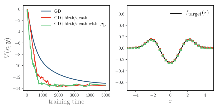
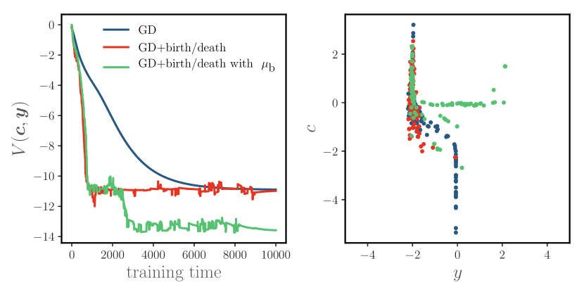
Figure 1: Top left: Convergence of the gradient descent dynamics without birth-death, with birth-death, and using a reinjection distribution. Top right: For appropriate initialization, the three dynamical schemes all converge to the target function. Bottom left: For bad initialization (narrow Gaussian distributed around y=-2), GD and GD+birth-death do not converge on this timescale. Interestingly, with the reinjection via distribution $\mu_{\textrm{b}}$, convergence to the global minimum is rapidly achieved. Bottom right: The configuration of the particles in $\boldsymbol{\theta}=(y,c)$. Only with the reinjection distribution does mass exist near $y=2$.

7.2 Student-Teacher ReLU Network

In many optimization problems, it is not possible to evaluate $\tilde{V}$ exactly. Instead, typically $\tilde{V}$ is estimated as a sample mean over a batch of data. We consider a student-teacher set-up similar to [CB18a] in which we use single hidden layer ReLU networks to approximate a network of the same type with fewer neurons. We use as the target function a ReLU network with 50-$d$ input and 10 hidden units. We approximate the teacher with neural networks with $n=50$ neurons (see SM). The networks are trained with stochastic gradient descent (SGD) and the mini-batch estimate of the gradient of output layer, which is computed at each step of SGD, is used to compute $\tilde{V},$ which determines the rate of birth-death. In experiments with the reinjection distribution, we use (43) with Gaussian $\bar{\rho}.$

As shown in Fig. 2, we find that the birth-death dynamics accelerates convergence to the teacher network. We emphasize that because the birth-death dynamics is stochastic at finite particle numbers, the fluctuations associated with the process could be unfavorable in some cases. In such situations, it is useful to reduce $\alpha$ as a function of time. On the other hand, in some cases we have observed much more dramatic accelerations from the birth-death dynamics.

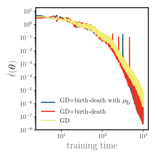
Figure 2: The batch loss as a function of training time for the student-teacher ReLU network described in Sec. 7.2. The birth-death dynamics accelerates convergence, both with and without the reinjection distribution.

8 Conclusions

The success of an optimization algorithm based on gradient descent requires good coverage of the parameter space so that local updates can reach the minima of the loss function quickly. Our approach liberates the parameters from a purely local dynamics and allows rapid reallocation to values at which they can best reduce the approximation error. Importantly, we have constructed the non-local birth-death dynamics so that it converges to the minimizers of the loss function. For a very general class of minimization problems—both interacting and non-interacting potentials—we have established convergence to energy minimizers under the dynamics described by the mean-field PDE with birth-death. Remarkably, for interacting systems with we can guarantee global convergence for sufficiently regular initial conditions. We have also computed the asymptotic rate of convergence with birth-death dynamics.

These theoretical results translate to dramatic reductions in convergence time for our illustrative examples. It is worth emphasizing that the schemes we have described are straightforward to implement and come with little computational overhead. Extending this type of dynamics to deep neural network architectures could accelerate the slow dynamics at the initial layers often observed in practice. Hyperparameter selection strategies based on evolutionary algorithms [SMC⁺17] provide another interesting potential application of our approach.

While we have characterized the basic behavior of optimization under the birth-death dynamics, many theoretical questions remain. First, we did not address generalization; understanding the role of the extra birth/death term in controlling the generalization gap is an important future question, in particular relating it to the lazy-training regime of [CB18a]. Next, we need to assume the existence of weak solutions through (14) with an initial measure $\mu_{0}$ that has full support, yet it may be possible to certify that the dynamics exist for all times if $\mu_{0}$ decays sufficiently fast. Besides, more explicit calculations of global convergence rates for the interacting case and tighter rates for the non-interacting case would be exciting additions. The proper choice of $\mu_{\textrm{b}}$ is another question worth exploring because, as highlighted in our simple example, favorable reinjection distributions can rapidly overcome slow dynamics. Finally, a mean-field perspective on deep neural networks would enable us to translate some of the guarantees here to deep architectures.

Appendix A Generalizations of (13)

Here we mention two ways in which we can modify (13) to certain advantages. For example, we can replace this equation with

$$\partial_{t}\mu_{t}=\nabla\cdot\left(\mu_{t}\nabla V\right)-\alpha f(V-\bar{V})\mu_{t}-\bar{f}\mu_{t},$$ (54)

where $f:\mathbb{R}\to\mathbb{R}$ is some function and $\bar{f}=\int_{D}f(V-\bar{V})d\mu_{t}$. As we will see in Proposition A.1, as long as $zf(z)\geq 0$ for all $z\in\mathbb{R}$, the additional term in (54) increase the rate of decay of the energy.

While the birth-death dynamics described above ensures convergence in the mean-field limit, when $n$ is finite, particles can only be created in proportion to the empirical distribution $\mu^{(n)}.$ In particular, such a birth process corresponds to “cloning” or creating identical replicas of existing particles. In practice, there may be an advantage to exploring parameter space with a distribution distinct from the instantaneous empirical particle distribution (7). To enable this exploration we introduce a birth term proportional to a distribution $\mu_{\textrm{b}}$ which we will assume has full support on $D$. In this case, the time evolution of the distribution is described by

$$\partial_{t}\mu_{t}=\nabla\cdot\left(\mu_{t}\nabla V\right) -\alpha(V-\bar{V})_{+}\mu_{t}+\alpha\left({\textstyle\int_{D}(V-\bar{V})_{+}d\mu_{t}}\right)\frac{\mu_{\textrm{b}}\mathbbm{1}_{V\leq\bar{V}}}{\mu_{b}(V\leq\bar{V})}$$ (55)

$$+\alpha^{\prime}(V-\bar{V})_{-}\mu_{\textrm{b}}-\alpha^{\prime}\left({\textstyle\int_{D}(V-\bar{V})_{-}d\mu_{\text{b}}}\right)\frac{\mu_{t}\mathbbm{1}_{V>\bar{V}}}{\mu_{t}(V>\bar{V})},$$

where $\alpha,\alpha^{\prime}>0$, $(V-\bar{V})_{+}=\max(V-\bar{V},0)\geq 0$, $(V-\bar{V})_{-}=\max(\bar{V}-V,0)\geq 0$. That is, we kill particles in proportion to $\mu_{t}$ in region where $V>\bar{V}$ but create new particles from $\mu_{\textrm{b}}$ in regions where $V\leq\bar{V}$. We could also combine (54) with (55) to obtain other variants.

These alternative birth-death dynamical schemes also satisfy the consistency conditions of Proposition 3.1:

Proposition A.1

Let $\mu_{t}$ be a solution of (54) with $f$ such that $zf(z)\geq 0$ for all $z\in\mathbb{R}$ or (55), with $\mu_{0}\in\mathcal{M}(D)$. Then, $\mu_{t}(D)=1$ for all $t\geq 0$, and ${E}(t)=\mathcal{E}[\mu_{t}]$ satisfies

$$\dot{{E}}(t)\leq-\int_{D}|\nabla V(\boldsymbol{\theta},[\mu_{t}])|^{2}\mu_{t}(d\boldsymbol{\theta})\,.$$ (56)

Proof: By considering again $1$ and $V(\cdot,[\mu_{t}])$ as a test function in (54) or (55), we verify that $\partial_{t}\mu_{t}(D)=0$. In addition, (54) implies that

$$\dot{E}(t) =\int_{D}V(\boldsymbol{\theta},[\mu_{t}])\partial_{t}\mu_{t}(d\boldsymbol{\theta})$$

$$=\int_{D}\left(V(\boldsymbol{\theta},[\mu_{t}])-\bar{V}[\mu_{t}]\right)\partial_{t}\mu_{t}(d\boldsymbol{\theta})$$

$$=-\int_{D}|\nabla V|^{2}d\mu_{t}-\alpha\int_{D}(V-\bar{V})f(V-\bar{V})d\mu_{t}$$

which proves (56) for (54) since all the terms at the right hand side of this equation are negative individually if $zf(z)\geq 0$ for all $z\in\mathbb{R}$. Similarly, (55) implies that

$$\dot{E}(t) =\int_{D}V(\boldsymbol{\theta},[\mu_{t}])\partial_{t}\mu_{t}(d\boldsymbol{\theta})$$

$$=\int_{D}\left(V(\boldsymbol{\theta},[\mu_{t}])-\bar{V}[\mu_{t}]\right)\partial_{t}\mu_{t}(d\boldsymbol{\theta})$$

$$=-\int_{D}|\nabla V|^{2}d\mu_{t}-\alpha\int_{D}(V-\bar{V})^{2}_{+}d\mu_{t}-\alpha\frac{\int_{D}(V-\bar{V})_{+}d\mu_{t}\int_{D}(V-\bar{V})_{-}d\mu_{\textrm{b}}}{\mu_{b}(V\leq 0)}$$

$$\quad-\alpha^{\prime}\int_{D}(V-\bar{V})^{2}_{-}d\mu_{\textrm{b}}-\alpha^{\prime}\frac{\int_{D}(V-\bar{V})_{-}d\mu_{\textrm{b}}\int_{D}(V-\bar{V})_{+}d\mu_{t}}{\mu_{t}(V>0)},$$

which proves (56) for (55) since all the terms at the right hand side of this equation are negative. $\square$

Appendix B Convergence and Rates in the Non-interacting Case

B.1 Non-interacting Case without the Transportation Term

Let us look first at the PDE satisfied by the measure $\mu$ in the non-interacting case, i.e. with $V=F$ satisfying Assumption 4.1, and without the transportation term:

$$\partial_{t}\mu_{t}=-\alpha F(\boldsymbol{\theta})\mu_{t}+\alpha\bar{F}(t)\mu_{t},$$ (57)

where $\bar{F}(t)=\int_{\mathbb{R}^{k}}F(\boldsymbol{\theta})\mu_{t}(d\boldsymbol{\theta})$. This equation can be solved exactly. Assuming that $\mu_{0}$ has a density everywhere positive on $\mathbb{R}^{k}$, $\mu_{t}$ has a density $\rho_{t}$ given by

$$\rho_{t}(\boldsymbol{\theta})=e^{\alpha\int_{0}^{t}\bar{F}(s)ds-\alpha tF(\boldsymbol{\theta})}\rho_{0}(\boldsymbol{\theta}).$$ (58)

The normalization condition $\mu_{t}(\mathbb{R}^{k})=\int_{\mathbb{R}^{k}}\rho_{t}(\boldsymbol{\theta})d\boldsymbol{\theta}=1$ leads to:

$$e^{\alpha\int_{0}^{t}\bar{F}(s)ds}\int_{\mathbb{R}^{k}}e^{-\alpha tF(\bm{\theta^{\prime}})}\rho_{0}(\boldsymbol{\theta}^{\prime})d\boldsymbol{\theta}^{\prime}=1$$

$$\Leftrightarrow\quad e^{-\alpha\int_{0}^{t}\bar{F}(s)ds}=\int_{\mathbb{R}^{k}}e^{-\alpha tF(\bm{\theta^{\prime}})}\rho_{0}(\boldsymbol{\theta}^{\prime})d\boldsymbol{\theta}^{\prime}.$$

Therefore, by plugging this last expression in equation (58), we obtain the explicit expression

$$\rho_{t}(\boldsymbol{\theta})=\frac{e^{-\alpha tF(\boldsymbol{\theta})}\rho_{0}(\boldsymbol{\theta})}{\int_{\mathbb{R}^{k}}e^{-\alpha tF(\boldsymbol{\theta}^{\prime})}\rho_{0}(\boldsymbol{\theta}^{\prime})d\boldsymbol{\theta}^{\prime}}.$$ (59)

We can use this equation to express the energy $\bar{F}(t)=\int_{\mathbb{R}^{k}}F(\boldsymbol{\theta})\rho_{t}(\boldsymbol{\theta})d\boldsymbol{\theta}$:

$$\bar{F}(t)=\frac{\int_{\mathbb{R}^{k}}F(\boldsymbol{\theta})e^{-\alpha tF(\boldsymbol{\theta})}\rho_{0}(\boldsymbol{\theta})d\boldsymbol{\theta}}{\int_{\mathbb{R}^{k}}e^{-\alpha tF(\boldsymbol{\theta})}\rho_{0}(\boldsymbol{\theta})d\boldsymbol{\theta}}=\frac{d}{d\alpha t}G(\alpha t),$$ (60)

where $G(\alpha t)$ is the function defined as:

$$G(\alpha t)=-\log\int_{\mathbb{R}^{k}}e^{-\alpha tF(\boldsymbol{\theta})}\rho_{0}(\boldsymbol{\theta})d\boldsymbol{\theta}.$$ (61)

At late times, the factor $e^{-\alpha tF(\boldsymbol{\theta})}$ focuses all the mass in the vicinity of the global minimum of $F$. Therefore, we can neglect the influence of the density $\rho_{0}$ in this integral. More precisely a calculation using the Laplace method indicates that

$$\int_{\mathbb{R}^{k}}e^{-\alpha tF(\boldsymbol{\theta})}d\boldsymbol{\theta}\sim(2\pi)^{d/2}(\alpha t)^{-d/2}(\det(H^{*}))^{-1/2}.$$ (62)

where $H^{*}=\nabla\nabla F(\boldsymbol{\theta}^{*})$ is the Hessian at the global minimum located at $\boldsymbol{\theta}^{*}$, and $\sim$ indicates that the ratio of both sides of the equation tend to 1 as $\alpha t\to\infty$. This shows that

$$\bar{F}(t)\sim\tfrac{1}{2}d(\alpha t)^{-1}\qquad\text{as \ \ $\alpha t\to\infty$}$$ (63)

B.2 Non-interacting Case with Transportation and Birth-death

B.2.1 Proof of Theorem 4.2

We first prove the following intermediate result

Lemma B.1

Let $\delta>0$ arbitrary, and define

$$\phi_{\delta}(\boldsymbol{\theta})=\max(0,1-\delta^{-1}F(\boldsymbol{\theta}))~{},~{}f_{\delta}=\int_{\mathbb{R}^{k}}\phi_{\delta}(\boldsymbol{\theta})\mu_{0}(d\boldsymbol{\theta})~{}.$$

Then

$$\forall t\ :\quad E(t)\leq\delta+\frac{1}{\alpha tf_{\delta}}~{}.$$ (64)

Proof: By slightly abusing notation, we define

$$f_{\delta}(t)=\int_{\mathbb{R}^{k}}\phi_{\delta}(\boldsymbol{\theta})\mu_{t}(d\boldsymbol{\theta})~{}.$$

We consider the following Lyapunov function:

$$\mathcal{L}_{\delta}(t)=\alpha t(E(t)-\delta)+\frac{1}{f_{\delta}(t)}~{}.$$ (65)

Its time derivative is

$$\dot{\mathcal{L}}_{\delta}(t)=\alpha(E(t)-\delta)+\alpha t\dot{E}(t)-\frac{\dot{f_{\delta}}(t)}{f_{\delta}^{2}(t)}~{}.$$ (66)

By definition, we have

$$\dot{E}(t)=-\int_{\mathbb{R}^{k}}|\nabla F(\boldsymbol{\theta})|^{2}\mu_{t}(d\boldsymbol{\theta})-\alpha\int_{\mathbb{R}^{k}}(F(\boldsymbol{\theta})-F(t))^{2}\mu_{t}(d\boldsymbol{\theta})\leq 0~{}.$$ (67)

We also have

$$\dot{f}_{\delta}(t) =-\int_{\mathbb{R}^{k}}\langle\nabla\phi_{\delta}(\boldsymbol{\theta}),\nabla F(\boldsymbol{\theta})\rangle\mu_{t}(d\boldsymbol{\theta})-\alpha\int_{\mathbb{R}^{k}}\phi_{\delta}(\boldsymbol{\theta})F(\boldsymbol{\theta})\mu_{t}(d\theta)+\alpha E(t)f_{\delta}(t)$$

$$\geq\delta^{-1}\int_{\mathbb{R}^{k}}|\nabla F(\boldsymbol{\theta})|^{2}\mu_{t}(d\boldsymbol{\theta})+\alpha(E(t)-\delta)f_{\delta}(t)$$

$$\geq\alpha(E(t)-\delta)f_{\delta}(t)~{}.$$ (68)

Observe that $0\leq f_{\delta}(t)<1$ because otherwise $F$ would be flat (in which case the energy is $0$). Also, we can assume wlog that $E(t)-\delta>0$, since otherwise the statement of the lemma is trivially verified. By plugging (67) and (B.2.1) into (66) we have

$$\dot{\mathcal{L}}_{\delta}(t)\leq\alpha(E(t)-\delta)-\alpha(E(t)-\delta)f_{\delta}^{-1}(t)=\alpha(E(t)-\delta)(1-f_{\delta}^{-1}(t))\leq 0~{}.$$ (69)

Finally, since $f^{-1}_{\delta}(t)\geq 0$, we have

$$(E(t)-\delta)\leq\frac{\mathcal{L}_{\delta}(t)}{\alpha t}\leq\frac{\mathcal{L}_{\delta}(0)}{\alpha t}=\frac{1}{\alpha tf_{\delta}}~{},$$

which concludes the proof of the Lemma. $\square$

Proof of Theorem 4.2: In order to prove (27), we apply the previous lemma for $\delta\to 0$. Let $\theta^{*}=\arg\min V(\theta)$, We have $F(\boldsymbol{\theta}^{*})=0$, and $\|\nabla\nabla F(\boldsymbol{\theta})\|\leq\beta$ for some $\beta>0$. Then, for $\delta$ sufficiently small, the indicator function $\phi_{\delta}(\boldsymbol{\theta})$ is localized in the set

$$\left\{\boldsymbol{\theta}\in\mathbb{R}^{k};\tfrac{1}{2}\langle(\boldsymbol{\theta}-\boldsymbol{\theta}^{*}),H^{*}(\boldsymbol{\theta}-\boldsymbol{\theta}^{*})\leq\delta\right\}\supseteq\left\{\boldsymbol{\theta}\in\mathbb{R}^{d};\|\boldsymbol{\theta}-\boldsymbol{\theta}^{*}\|^{2}\leq 2\beta^{-1}\delta\right\}~{}.$$

where $H^{*}=\nabla\nabla F(\boldsymbol{\theta}^{*})$. It follows that for sufficiently small $\delta$,

$$f_{\delta} =\int_{\mathbb{R}^{k}}\phi_{\delta}(\boldsymbol{\theta})\mu_{0}(d\boldsymbol{\theta})$$

$$\gtrsim\rho_{0}(\boldsymbol{\theta}^{*})\int_{\|\boldsymbol{\theta}-\boldsymbol{\theta}^{*}\|\leq\sqrt{2\beta^{-1}\delta}}\left(1-\tfrac{1}{2}\delta^{-1}\langle(\boldsymbol{\theta}-\boldsymbol{\theta}^{*}),H^{*}(\boldsymbol{\theta}-\boldsymbol{\theta}^{*})\rangle\right)d\boldsymbol{\theta}$$

$$\sim\rho_{0}(\boldsymbol{\theta}^{*})\left(2\beta^{-1}\delta\right)^{d/2}~{}.$$ (70)

By plugging (B.2.1) into (64) we obtain

$$\forall\,\delta,t>0\ :\qquad~{}E(t)\leq\delta+\frac{1}{\alpha t}\left(\frac{\beta}{2\delta}\right)^{d/2}\sim\delta+C\delta^{-d/2}t^{-1}~{},$$

which implies that in order to reach an error $\epsilon$, we need

$$t_{\epsilon}=O\left(\epsilon^{-(d+2)/2}\right)~{},$$

which shows (27).

To obtain the asymptotic convergence rate in (28), note that by Lemma B.2 below the energy $\bar{F}(t)=\int_{\mathbb{R}^{k}}F(\boldsymbol{\theta})\rho_{t}(\boldsymbol{\theta})d\boldsymbol{\theta}$ can be written in terms of (77) as

$$\bar{F}(t)=\frac{\int_{\mathbb{R}^{k}}F(\boldsymbol{\theta})\exp\left(\int_{-t}^{0}(-\alpha F(\boldsymbol{\Theta}(s,\boldsymbol{\theta}))+\Delta F(\boldsymbol{\Theta}(s,\boldsymbol{\theta})))ds\right)\rho_{0}(\boldsymbol{\Theta}(-t,\boldsymbol{\theta}))d\boldsymbol{\theta}}{\int_{\mathbb{R}^{k}}\exp\left(\int_{-t}^{0}(-\alpha F(\boldsymbol{\Theta}(s,\boldsymbol{\theta}))+\Delta F(\boldsymbol{\Theta}(s,\boldsymbol{\theta})))ds\right)\rho_{0}(\boldsymbol{\Theta}(-t,\boldsymbol{\theta}))d\boldsymbol{\theta}}$$ (71)

For large $t$, we can again use Laplace method to confirm that $\rho(t,\boldsymbol{\theta})$ concentrates near the absolute minimum of $F(\boldsymbol{\theta})$ located at $\boldsymbol{\theta}^{*}$. To see why notice that $\boldsymbol{\Theta}(t,\boldsymbol{\theta})$ converge, as $t\to\infty$, near local minima of $F$. Suppose that these minima are located at $\boldsymbol{\theta}_{1}^{*}=\boldsymbol{\theta}^{*}$, $\boldsymbol{\theta}_{2}^{*}$, etc. At these minima we have $\nabla F(\boldsymbol{\theta}^{*}_{j})=0$, and if in (79) we replace $F(\boldsymbol{\theta})$ by its quadratic approximation around any $\boldsymbol{\theta}_{j}^{*}$, $\tfrac{1}{2}\langle\boldsymbol{\theta}-\boldsymbol{\theta}_{j}^{*},H_{j}^{*}(\boldsymbol{\theta}-\boldsymbol{\theta}_{j}^{*})\rangle$ with $H_{j}^{*}=\nabla\nabla H(\boldsymbol{\theta}_{j}^{*})$ positive definite, the solution to this equation reads

$$\boldsymbol{\Theta}^{j}_{\text{quad}}(t,\boldsymbol{\theta})=\boldsymbol{\theta}_{j}^{*}+e^{-H^{*}t}(\boldsymbol{\theta}-\boldsymbol{\theta}_{j}^{*})$$ (72)

from which we deduce

$$\int_{-t}^{0}\Delta F(\boldsymbol{\Theta}^{j}_{\text{quad}}(s,\boldsymbol{\theta}))ds=\operatorname{tr}(H_{j}^{*})t,$$ (73)

and

$$-\alpha\int_{-t}^{0}F(\boldsymbol{\Theta}^{j}_{\text{quad}}(s,\boldsymbol{\theta}))ds =\alpha F(\boldsymbol{\theta}^{*}_{j})t-\tfrac{1}{2}\alpha\int_{-t}^{0}\langle\tilde{\boldsymbol{\theta}}_{j},e^{-H^{*}s}H^{*}e^{-H^{*}s}\tilde{\boldsymbol{\theta}}_{j}\rangle$$ (74)

$$=\alpha F(\boldsymbol{\theta}^{*}_{j})t-\tfrac{1}{4}\alpha\langle\tilde{\boldsymbol{\theta}}_{j},(e^{2H^{*}t}-\mathrm{Id})\tilde{\boldsymbol{\theta}}_{j}\rangle.$$

where $\tilde{\boldsymbol{\theta}}_{j}=\boldsymbol{\theta}-\boldsymbol{\theta}_{j}^{*}$. Since $F(\boldsymbol{\theta}_{j}^{*})>0$ except for the the global minimum $F(\boldsymbol{\theta}_{1}^{*})=F(\boldsymbol{\theta}_{1}^{*})=0$, for large $t$, the only points that contribute to the integrals in (71) are those in a small region near $\boldsymbol{\theta}^{*}$ where we can replace $\boldsymbol{\Theta}(t,\boldsymbol{\theta})$ by $\boldsymbol{\Theta}^{1}_{\text{quad}}(t,\boldsymbol{\theta})$. As a result we can again neglect $\rho_{0}$ in these integrals, and evaluate them as if $\rho_{t}$ was asymptotically the Gaussian density:

$$\rho_{t}(\boldsymbol{\theta})\sim\mathcal{N}(\boldsymbol{\theta}^{*},2\alpha^{-1}e^{-2H^{*}t}).$$ (75)

This quantifies the late stages of the global convergence to the minimum and confirms the asymptotic decay rate in (28), thereby concluding the proof of Theorem 4.2. $\square$

Lemma B.2

Denote by $\boldsymbol{\Theta}(t,\boldsymbol{\theta})$ the solution of the ODE

$$\dot{\boldsymbol{\Theta}}(t,\boldsymbol{\theta})=-\nabla F(\boldsymbol{\Theta}(t,\boldsymbol{\theta})),\qquad\boldsymbol{\Theta}(0,\boldsymbol{\theta})=\boldsymbol{\theta}$$ (76)

Then under the conditions of Theorem 4.2, the solution $\mu_{t}$ of the PDE (12) has a density $\rho_{t}$ given by

$$\rho_{t}(\boldsymbol{\theta})=\frac{\exp\left(\int_{-t}^{0}G(\Theta(s,\boldsymbol{\theta}))ds\right)\rho_{0}(\boldsymbol{\Theta}(-t,\boldsymbol{\theta}))}{\int_{D}\exp\left(\int_{-t}^{0}G(\Theta(s,\boldsymbol{\theta}^{\prime}))ds\right)\rho_{0}(\boldsymbol{\Theta}(-t,\boldsymbol{\theta}^{\prime}))d\boldsymbol{\theta}^{\prime}}$$ (77)

where $G(\boldsymbol{\theta})=\Delta F(\boldsymbol{\theta})-\alpha F(\boldsymbol{\theta})$.

Proof: Since the initial $\mu_{0}$ has a density $\rho_{0}>0$, so does $\mu_{t}$ for all $t>0$ (but not in the limit as $t\to\infty$) and its density satisfies

$$\partial_{t}\rho_{t} =\nabla\cdot\left(\rho_{t}\nabla F(\boldsymbol{\theta})\right)-\alpha F(\boldsymbol{\theta})\rho_{t}+\alpha\bar{F}(t)\rho(t),$$ (78)

If $\boldsymbol{\Theta}(t,\boldsymbol{\theta})$ satisfies

$$\dot{\boldsymbol{\Theta}}(t,\boldsymbol{\theta})=-\nabla F(\boldsymbol{\Theta}(t,\boldsymbol{\theta}))\qquad\boldsymbol{\Theta}(0,\boldsymbol{\theta})=\boldsymbol{\theta}.$$ (79)

we have

$$\frac{d}{dt}\rho_{t}(\boldsymbol{\Theta}(t,\boldsymbol{\theta})) =\partial_{t}\rho_{t}(\boldsymbol{\Theta}(t,\boldsymbol{\theta}))+\dot{\boldsymbol{\Theta}}(t,\boldsymbol{\theta}))\cdot\nabla\rho_{t}(\boldsymbol{\Theta}(t,\boldsymbol{\theta}))$$ (80)

$$=\Delta F(\boldsymbol{\Theta}(t,\boldsymbol{\theta}))\rho(t,\boldsymbol{\Theta}(t,\boldsymbol{\theta}))-\left(F(\boldsymbol{\Theta}(t,\boldsymbol{\theta}))-\alpha\bar{F}(t)\right)\rho_{t}(\boldsymbol{\Theta}(t,\boldsymbol{\theta})).$$

Therefore

$$\rho_{t}(\boldsymbol{\Theta}(t,\boldsymbol{\theta}))=\exp\left(\int_{0}^{t}(-\alpha F(\boldsymbol{\Theta}(s,\boldsymbol{\theta}))+\alpha\bar{F}(s)+\Delta F(\boldsymbol{\Theta}(s,\boldsymbol{\theta})))ds\right)\rho_{0}(\boldsymbol{\theta}).$$ (81)

By using $\boldsymbol{\Theta}(t,\boldsymbol{\Theta}(s,\boldsymbol{\theta}))=\boldsymbol{\Theta}(t+s,\boldsymbol{\theta})$ and the normalization condition, this implies

$$\rho_{t}(\boldsymbol{\theta})=\frac{\exp\left(\int_{-t}^{0}(-\alpha F(\boldsymbol{\Theta}(s,\boldsymbol{\theta}))+\Delta F(\boldsymbol{\Theta}(s,\boldsymbol{\theta})))ds\right)\rho_{0}(\boldsymbol{\Theta}(-t,\boldsymbol{\theta}))}{\int_{\mathbb{R}^{k}}\exp\left(\int_{-t}^{0}(-\alpha F(\boldsymbol{\Theta}(s,\boldsymbol{\theta}^{\prime}))+\Delta F(\boldsymbol{\Theta}(s,\boldsymbol{\theta}^{\prime})))ds\right)\rho_{0}(\boldsymbol{\Theta}(-t,\boldsymbol{\theta}^{\prime}))d\boldsymbol{\theta}^{\prime}}.$$ (82)

This is (77) and terminates the proof of the lemma. $\square$

Appendix C Derivation of (30)

Let $\mu_{*}$ be a minimizer and compare its energy to that of any other probability measure $\mu$. Since the energy minimum is unique by convexity, we must have $\mathcal{E}[\mu]\geq\mathcal{E}[\mu_{*}]$. A direct calculation shows that

$$\mathcal{E}[\mu] =\mathcal{E}[\mu_{*}]+\int_{D}V(\boldsymbol{\theta},[\mu_{*}])(\mu(d\boldsymbol{\theta})-\mu_{*}(d\boldsymbol{\theta}))$$ (83)

$$\quad+\tfrac{1}{2}\int_{D\times D}K(\boldsymbol{\theta},\boldsymbol{\theta}^{\prime})(\mu(d\boldsymbol{\theta})-\mu_{*}(d\boldsymbol{\theta}))(\mu(d\boldsymbol{\theta}^{\prime})-\mu_{*}(d\boldsymbol{\theta}^{\prime}))$$

The last term at the right hand side is always non-negative. Focusing on the second term, if we denote $\operatorname{supp}\mu_{*}=D_{*}$, we can write it as

$$\int_{D}V(\boldsymbol{\theta},[\mu_{*}])(\mu(d\boldsymbol{\theta})-\mu_{*}(d\boldsymbol{\theta})) =\int_{D}\left(V(\boldsymbol{\theta},[\mu_{*}])-\bar{V}[\mu_{*}])\right)(\mu(d\boldsymbol{\theta})-\mu_{*}(d\boldsymbol{\theta}))$$ (84)

$$=\int_{D_{*}^{c}}\left(V(\boldsymbol{\theta},[\mu_{*}])-\bar{V}[\mu_{*}])\right)\mu(d\boldsymbol{\theta})$$

where we used $V(\boldsymbol{\theta},[\mu_{*}])=\bar{V}[\mu_{*}]$ on $D_{*}$ and $\mu_{*}=0$ on $D_{*}^{c}$. The only possibility to make this term nonnegative for all $\mu$ is to have $V(\boldsymbol{\theta},[\mu_{*}])\geq\bar{V}[\mu_{*}]$ on $D_{*}^{c}$.

Appendix D Proof of Theorem 4.5

We begin by noting that, if (14) holds for al $t>0$, then $\bar{V}[\mu_{t}]=-\alpha^{-1}d\log C(t)/dt$ must be well-defined at all times. From (15), this derivative is given by

$$\bar{V}[\mu_{t}]=-\alpha^{-1}\frac{d}{dt}\log C(t)=\frac{\int_{D}V(\boldsymbol{\Theta}(t,\boldsymbol{\theta}),[\mu_{t}])e^{-\alpha\int_{0}^{t}V(\boldsymbol{\Theta}(s,\boldsymbol{\theta}),[\mu_{s}])ds}\mu_{0}(d\boldsymbol{\theta})}{\int_{D}e^{-\alpha\int_{0}^{t}V(\boldsymbol{\Theta}(s,\boldsymbol{\theta}),[\mu_{s}])ds}\mu_{0}(d\boldsymbol{\theta})}$$ (85)

Differentiating one more times gives

$$\frac{d}{dt}\bar{V}[\mu_{t}] =-\alpha\frac{\int_{D}|V(\boldsymbol{\Theta}(t,\boldsymbol{\theta}),[\mu_{t}])|^{2}e^{-\alpha\int_{0}^{t}V(\boldsymbol{\Theta}(s,\boldsymbol{\theta}),[\mu_{s}])ds}\mu_{0}(d\boldsymbol{\theta})}{\int_{D}e^{-\alpha\int_{0}^{t}V(\boldsymbol{\Theta}(s,\boldsymbol{\theta}),[\mu_{s}])ds}\mu_{0}(d\boldsymbol{\theta})}$$ (86)

$$\quad+\alpha\left(\frac{\int_{D}V(\boldsymbol{\Theta}(t,\boldsymbol{\theta}),[\mu_{t}])e^{-\alpha\int_{0}^{t}V(\boldsymbol{\Theta}(s,\boldsymbol{\theta}),[\mu_{s}])ds}\mu_{0}(d\boldsymbol{\theta})}{\int_{D}e^{-\alpha\int_{0}^{t}V(\boldsymbol{\Theta}(s,\boldsymbol{\theta}),[\mu_{s}])ds}}\right)^{2}$$

$$\quad+\frac{\int_{D}\partial_{t}V(\boldsymbol{\Theta}(t,\boldsymbol{\theta}),[\mu_{t}])e^{-\alpha\int_{0}^{t}V(\boldsymbol{\Theta}(s,\boldsymbol{\theta}),[\mu_{s}])ds}\mu_{0}(d\boldsymbol{\theta})}{\int_{D}e^{-\alpha\int_{0}^{t}V(\boldsymbol{\Theta}(s,\boldsymbol{\theta}),[\mu_{s}])ds}\mu_{0}(d\boldsymbol{\theta})}$$

$$=-\alpha\frac{\int_{D}|V(\boldsymbol{\Theta}(t,\boldsymbol{\theta}),[\mu_{t}])|^{2}e^{-\alpha\int_{0}^{t}V(\boldsymbol{\Theta}(s,\boldsymbol{\theta}),[\mu_{s}])ds}\mu_{0}(d\boldsymbol{\theta})}{\int_{D}e^{-\alpha\int_{0}^{t}V(\boldsymbol{\Theta}(s,\boldsymbol{\theta}),[\mu_{s}])ds}\mu_{0}(d\boldsymbol{\theta})}$$

$$\quad+\alpha\left(\frac{\int_{D}V(\boldsymbol{\Theta}(t,\boldsymbol{\theta}),[\mu_{t}])e^{-\alpha\int_{0}^{t}V(\boldsymbol{\Theta}(s,\boldsymbol{\theta}),[\mu_{s}])ds}\mu_{0}(d\boldsymbol{\theta})}{\int_{D}e^{-\alpha\int_{0}^{t}V(\boldsymbol{\Theta}(s,\boldsymbol{\theta}),[\mu_{s}])ds}}\right)^{2}$$

$$\quad+\frac{\int_{D}\dot{\boldsymbol{\Theta}}(t,\boldsymbol{\theta})\cdot\nabla V(\boldsymbol{\Theta}(t,\boldsymbol{\theta}),[\mu_{t}])e^{-\alpha\int_{0}^{t}V(\boldsymbol{\Theta}(s,\boldsymbol{\theta}),[\mu_{s}])ds}\mu_{0}(d\boldsymbol{\theta})}{\int_{D}e^{-\alpha\int_{0}^{t}V(\boldsymbol{\Theta}(s,\boldsymbol{\theta}),[\mu_{s}])ds}\mu_{0}(d\boldsymbol{\theta})}$$

$$\quad+\frac{\int_{D\times D}K(\boldsymbol{\Theta}(t,\boldsymbol{\theta}),\boldsymbol{\theta}^{\prime})\partial_{t}\mu_{t}(d\boldsymbol{\theta}^{\prime})e^{-\alpha\int_{0}^{t}V(\boldsymbol{\Theta}(s,\boldsymbol{\theta}),[\mu_{s}])ds}\mu_{0}(d\boldsymbol{\theta})}{\int_{D}e^{-\alpha\int_{0}^{t}V(\boldsymbol{\Theta}(s,\boldsymbol{\theta}),[\mu_{s}])ds}\mu_{0}(d\boldsymbol{\theta})}$$

Using (16) to replace $\dot{\boldsymbol{\Theta}}(t,\boldsymbol{\theta})$ by $-\nabla V(\boldsymbol{\Theta}(t,\boldsymbol{\theta}),[\mu_{t}])$ and (14) to express these integral as expectations against $\mu_{t}$ gives

$$\frac{d}{dt}\bar{V}[\mu_{t}] =-\alpha\int_{D}|V(\boldsymbol{\theta},[\mu_{t}])|^{2}\mu_{t}(d\boldsymbol{\theta})+\alpha\left(\int_{D}V(\boldsymbol{\theta},[\mu_{t}])\mu_{t}(d\boldsymbol{\theta})\right)^{2}$$ (87)

$$\quad-\int_{D}|\nabla V(\boldsymbol{\theta},[\mu_{t}])|^{2}\mu_{t}(d\boldsymbol{\theta})-\int_{D\times D}K(\boldsymbol{\theta},\boldsymbol{\theta}^{\prime})\partial_{t}\mu_{t}(d\boldsymbol{\theta}^{\prime})\mu_{t}(d\boldsymbol{\theta})$$

$$=-\alpha\int_{D}\left(V(\boldsymbol{\theta},[\mu_{t}])-\bar{V}[\mu_{t}]\right)^{2}\mu_{t}(d\boldsymbol{\theta})-\int_{D}|\nabla V(\boldsymbol{\theta},[\mu_{t}])|^{2}\mu_{t}(d\boldsymbol{\theta})$$

$$\quad-\tfrac{1}{2}\frac{d}{dt}\int_{D\times D}K(\boldsymbol{\theta},\boldsymbol{\theta}^{\prime})\mu_{t}(d\boldsymbol{\theta}^{\prime})\mu_{t}(d\boldsymbol{\theta})$$

Therefore the terms at right hand side of (17) must be well-defined and we must also have

$$\int_{D}|V(\boldsymbol{\theta},[\mu_{t}])|^{2}\mu_{t}(d\boldsymbol{\theta})<\infty,\qquad\int_{D}|\nabla V(\boldsymbol{\theta},[\mu_{t}])|^{2}\mu_{t}(d\boldsymbol{\theta})<\infty\qquad\int_{D\times D}K(\boldsymbol{\theta},\boldsymbol{\theta}^{\prime})\mu_{t}(d\boldsymbol{\theta}^{\prime})\mu_{t}(d\boldsymbol{\theta})<\infty$$ (88)

Since $\mu_{t}\rightharpoonup\mu_{*}\in\mathcal{M}(D)$ by assumption, we can take the limit as $t\to\infty$ to deduce that

$$\lim_{t\to\infty}\int_{D}V(\boldsymbol{\theta},[\mu_{t}])\mu_{t}(d\boldsymbol{\theta}) =\int_{D}V(\boldsymbol{\theta},[\mu_{*}])\mu_{*}(d\boldsymbol{\theta})$$ (89)

$$\lim_{t\to\infty}\int_{D}|V(\boldsymbol{\theta},[\mu_{t}])|^{2}\mu_{t}(d\boldsymbol{\theta}) =\int_{D}|V(\boldsymbol{\theta},[\mu_{*}])|^{2}\mu_{*}(d\boldsymbol{\theta})$$

$$\lim_{t\to\infty}\int_{D}|\nabla V(\boldsymbol{\theta},[\mu_{t}])|^{2}\mu_{t}(d\boldsymbol{\theta}) =\int_{D}|\nabla V(\boldsymbol{\theta},[\mu_{*}])|^{2}\mu_{*}(d\boldsymbol{\theta})$$

We will use these properties below, along with

$$V(\boldsymbol{\theta},[\mu_{t}])\to V(\boldsymbol{\theta},[\mu_{*}])\quad\text{and}\quad\int_{D}K(\boldsymbol{\theta},\boldsymbol{\theta}^{\prime})\mu_{t}(d\boldsymbol{\theta}^{\prime})\to\int_{D}K(\boldsymbol{\theta},\boldsymbol{\theta}^{\prime})\mu_{*}(d\boldsymbol{\theta}^{\prime})\qquad\text{pointwise in $D$}$$ (90)

which is require in order that both $\bar{V}[\mu_{t}]$ and $\mathcal{E}[\mu_{t}]$ be well-defined at all $t>0$ and in the limit as $t\to\infty$.

With these preliminaries, we now recall that the argument given after Theorem 4.5 implies that any fixed point $\mu_{*}$ of the PDE (13) must satisfy the first equation in (30). That is, we must have

$$V(\boldsymbol{\theta},[\mu_{*}])=\bar{V}[\mu_{*}]\qquad\forall\boldsymbol{\theta}\in\operatorname{supp}\mu_{*}$$ (91)

Therefore, to prove Theorem 4.5, it remains to show that the second equation in (30) must be satisfied as well. We will argue by contradiction: Let $D_{*}=\operatorname{supp}\mu_{*}$, assume $D_{*}^{c}\not=\emptyset$, and suppose that there exists a region $N\subseteq D_{*}^{c}$ where $V(\boldsymbol{\theta},[\mu_{*}])<\bar{V}[\mu_{*}]$. If it exists, this region must have nonzero Hausdorff measure in $D$ since, by Assumption 4.4, $V(\boldsymbol{\theta},[\mu_{t}])\in C^{2}(D)$ for all $t\geq 0$ and $V(\boldsymbol{\theta},[\mu_{*}])\in C^{2}(D)$. $V(\boldsymbol{\theta},[\mu_{*}])-\bar{V}[\mu_{*}]$ must also reach a minimum value inside $D$ even if $D$ is open, for otherwise (16) would eventually carry mass towards infinity, which contradicts $\mu_{t}\rightharpoonup\mu_{*}$. This implies that, if we pick $\delta\in(0,\bar{V}[\mu_{*}]-\min_{\boldsymbol{\theta}}V(\boldsymbol{\theta},[\mu_{*}]))$ and let

$$N_{\delta}=\{\boldsymbol{\theta}:\delta\leq\bar{V}[\mu_{*}]-V(\boldsymbol{\theta},[\mu_{*}])\}\subset N,$$ (92)

then $N_{\delta}$ is not empty. Since $V(\boldsymbol{\theta},[\mu_{*}])$ is twice differentiable in $\boldsymbol{\theta}$, for $\delta$ close enough to $\bar{V}[\mu_{*}]-\min_{\boldsymbol{\theta}}V(\boldsymbol{\theta},[\mu_{*}])$, $N_{\delta}$ is also compact and such that

$$\forall\boldsymbol{\theta}\in\partial N_{\delta}\ :\qquad|\nabla V(\boldsymbol{\theta},[\mu_{*}])|>0.$$ (93)

Given any solution $\mu_{t}$ of the PDE (13) that is supposed to converge to $\mu_{*}$ as $t\to\infty$, consider

$$f_{\delta}(t)=\mu_{t}(N_{\delta})$$ (94)

Since $\mu_{t}$ is positive everywhere at any finite time, we must have $f_{\delta}(t)>0$ for $t\in(0,\infty)$ However, since $\mu_{t}\to\mu_{*}$, we must also have

$$\lim_{t\to\infty}f_{\delta}(t)=0.$$ (95)

From (13), $f_{\delta}(t)$ satisfies

$$\dot{f}_{\delta}(t) =\int_{\partial N_{\delta}}\hat{n}\cdot\nabla Vd\sigma_{t}-\alpha\int_{N_{\delta}}(V-\bar{V})d\mu_{t}$$ (96)

where $\hat{n}(\boldsymbol{\theta})$ is the inward pointing unit normal to $\partial N_{\delta}$ at $\boldsymbol{\theta}$ and $\sigma_{t}$ is the probability measure on $\partial N_{\delta}$ obtained by restricting $\mu_{t}$ on this boundary: If $\phi_{\epsilon}\in C^{\infty}_{c}(D)$ is a sequence of test functions with $\operatorname{supp}\phi_{\epsilon}=N_{\delta}$ and converging towards the indicator set of $N_{\delta}$ as $\epsilon\to 0$, $\sigma_{t}$ is defined as

$$\lim_{\epsilon\to 0}\int_{N_{\delta}}\nabla\phi_{\epsilon}(\boldsymbol{\theta})\cdot\nabla V(\boldsymbol{\theta},[\mu_{t}])\mu_{t}(d\boldsymbol{\theta})=\int_{\partial N_{\delta}}\hat{n}(\boldsymbol{\theta})\cdot\nabla V(\boldsymbol{\theta},[\mu_{t}])d\sigma_{t}(\boldsymbol{\theta})$$ (97)

Since

$$\lim_{t\to\infty}\hat{n}(\boldsymbol{\theta})\cdot\nabla V(\boldsymbol{\theta},[\mu_{t}])=|\nabla V(\boldsymbol{\theta},[\mu_{*}])|>0,$$ (98)

there exists $t_{+}>0$ such that

$$\forall t>t_{+}\ :\qquad\int_{\delta N_{\delta}}\hat{n}\cdot\nabla Vd\nu_{t}>0.$$ (99)

Restricting ourselves to $t>t_{+}$, we therefore have

$$\dot{f}_{\delta}(t)>-\alpha\int_{N_{\delta}}(V-\bar{V})d\mu_{t}$$ (100)

Let us analyze the remaining integral in this equation. Denoting $\tilde{V}(\boldsymbol{\theta},[\mu_{t}])=V(\boldsymbol{\theta},[\mu_{t}])-\bar{V}[\mu_{t}]$, we have

$$-\alpha\int_{N_{\delta}}\tilde{V}(\boldsymbol{\theta},[\mu_{t}])\mu_{t}(d\boldsymbol{\theta}) =-\alpha\int_{N_{\delta}}\tilde{V}(\boldsymbol{\theta},[\mu_{*}])\mu_{t}(d\boldsymbol{\theta})$$ (101)

$$\quad-\alpha\int_{N_{\delta}}\left(\tilde{V}(\boldsymbol{\theta},[\mu_{t}])-\tilde{V}(\boldsymbol{\theta},[\mu_{*}])\right)\mu_{t}(d\boldsymbol{\theta})$$

$$\geq\alpha\delta f_{\delta}(t)-\alpha\int_{N_{\delta}}\left(\tilde{V}(\boldsymbol{\theta},[\mu_{t}])-\tilde{V}(\boldsymbol{\theta},[\mu_{*}])\right)\mu_{t}(d\boldsymbol{\theta})$$

where we used the definition of $N_{\delta}$. Looking at the last term, we can assess its magnitude using

$$\left|\int_{N_{\delta}}\left(\tilde{V}(\boldsymbol{\theta},[\mu_{t}])-\tilde{V}(\boldsymbol{\theta},[\mu_{*}])\right)\mu_{t}(d\boldsymbol{\theta})\right|$$ (102)

$$\leq\tfrac{1}{2}\int_{N_{\delta}}\left|\int_{D}K(\boldsymbol{\theta},\boldsymbol{\theta}^{\prime})\left(\mu_{t}(d\boldsymbol{\theta}^{\prime})-\mu_{*}(d\boldsymbol{\theta}^{\prime})\right)\right|\mu_{t}(d\boldsymbol{\theta})+\left|\bar{V}[\mu_{t}]-\bar{V}(\mu_{*})\right|f_{\delta}(t)$$

$$\leq M(t)f_{\delta}(t)$$

where (using the compactness of $N_{\delta}$)

$$M(t) =\max_{N_{\delta}}\left|\int_{D}K(\boldsymbol{\theta},\boldsymbol{\theta}^{\prime})(\mu_{t}(d\boldsymbol{\theta}^{\prime})-\mu_{*}(d\boldsymbol{\theta}^{\prime}))\right|+|\bar{V}[\mu_{t}]-\bar{V}(\mu_{*})|<\infty$$ (103)

Summarizing, we have deduced that

$$\dot{f}_{\delta}(t)>\alpha\delta f_{\delta}(t)+R(t)$$ (104)

with

$$|R(t)|\leq M(t)f_{\delta}(t)$$ (105)

Since we work under the assumption that $\mu_{t}\rightharpoonup\mu_{*}$, $M(t)$ must tend to $0$ as $t\to\infty$. As a result, $\exists t_{\delta}>0$ such $\forall t>t_{\delta}$ we have $N(t)<\delta$, which, from (104), implies that $\forall t>\max(t_{+},t_{\delta})$ we have $\dot{f}_{\delta}(t)>0$, a contradiction with (95). Therefore the only fixed points accessible by the PDE (13) are those for which both equations in (30) hold, which proves the theorem.

Appendix E Proof of Theorem 4.6

Let $\mu_{*}=\lim_{t\to\infty}\mu_{t}$ be the stationary point reached by the solution of (13) and denote $E(t)=\mathcal{E}[\mu_{t}]-\mathcal{E}[\mu_{*}]\geq 0$. Then

$$\frac{d}{dt}E^{-1} =-E^{-2}\int_{D}V\partial_{t}\mu_{t}$$ (106)

$$=E^{-2}\int_{D}\left(|\nabla V|^{2}+\alpha|V-\bar{V}|^{2}\right)d\mu_{t}$$

$$\geq\alpha E^{-2}\int_{D}|V-\bar{V}|^{2}d\mu_{t}$$

where we used $\int_{D}V^{2}d\mu_{t}-\bar{V}^{2}=\int_{D}|V-\bar{V}|^{2}d\mu_{t}$. By convexity

$$\mathcal{E}[\mu_{*}] \geq\mathcal{E}[\mu]-\int_{D}V(d\mu-d\mu_{*})$$ (107)

$$=\mathcal{E}[\mu]-\bar{V}+\int_{D}Vd\mu_{*}$$

$$=\mathcal{E}[\mu]+\int_{D}(V-\bar{V})d\mu_{*}$$

As a result

$$0\leq E\leq\int_{D}(\bar{V}-V)d\mu_{*}$$ (108)

and hence

$$0\leq E^{2}\leq\left|\int_{D}(V-\bar{V})d\mu_{*}\right|^{2}$$ (109)

Using this inequality in (106) gives

$$\frac{d}{dt}E^{-1}\geq\alpha\frac{\int_{D}|V-\bar{V}|^{2}d\mu_{t}}{\left|\int_{D}(V-\bar{V})d\mu_{*}\right|^{2}}$$ (110)

In Lemma E.1 below we show that $\exists t_{+}>0$ such that

$$\forall t>t_{+}\ :\ \frac{\int_{D}|V-\bar{V}|^{2}d\mu_{t}}{\left|\int_{D}(V-\bar{V})d\mu_{*}\right|^{2}}\geq C>0$$ (111)

As a result, $dE^{-1}/dt\geq\alpha$ for $t>t_{+}$. Integrating this relation in time on $[t_{0},t]$ with $t_{+}<t_{0}\leq t$ gives

$$E^{-1}(t)\geq E^{-1}(t)-E^{-1}(t_{0})\geq\alpha C(t-t_{0})$$ (112)

and hence

$$\lim_{t\to\infty}tE(t)\leq(\alpha C)^{-1}$$ (113)

which proves the theorem. $\square$

Note that the proof only takes into account the effects of birth-death terms; adding transport may accelerate the rate.

Lemma E.1

There exist $t_{+}>0$ such that (111) holds.

Proof: Let $\nu_{t}=\mu_{t}-\mu_{*}$ and for future reference note that $\nu_{t}$ is a signed measure on $D_{*}=\operatorname{supp}\mu_{*}$ but $\nu_{t}\geq 0$ on $D^{*}_{c}$. Denote

$$V=V(\boldsymbol{\theta},[\mu_{t}]),\qquad\bar{V}=\int_{D}V(\boldsymbol{\theta},[\mu_{t}])d\mu_{t},\qquad V_{*}=V(\boldsymbol{\theta},[\mu_{*}]),\qquad\bar{V}_{*}=\int_{D}V(\boldsymbol{\theta},[\mu_{*}])d\mu_{*}$$ (114)

We have

$$V =F(\boldsymbol{\theta})+\int_{D}K(\boldsymbol{\theta},\boldsymbol{\theta}^{\prime})(\mu_{*}(d\boldsymbol{\theta}^{\prime})+\nu_{t}(d\boldsymbol{\theta})^{\prime})$$ (115)

$$=V_{*}+\int_{D}K(\boldsymbol{\theta},\boldsymbol{\theta}^{\prime})\nu_{t}(d\boldsymbol{\theta}^{\prime})$$

and hence

$$\int_{D}Vd\mu_{*}=\bar{V}_{*}+\int_{D\times D}K(\boldsymbol{\theta},\boldsymbol{\theta}^{\prime})\nu_{t}(d\boldsymbol{\theta}^{\prime})\mu_{*}(d\boldsymbol{\theta})$$ (116)

Recall that $V_{*}=\bar{V}_{*}$ on $\operatorname{supp}\mu_{*}$. As a result

$$\bar{V} =\int_{D}F(\boldsymbol{\theta})(\mu_{*}(d\boldsymbol{\theta})+\nu_{t}(d\boldsymbol{\theta}))+\int_{D\times D}K(\boldsymbol{\theta},\boldsymbol{\theta}^{\prime})(\mu_{*}(d\boldsymbol{\theta})+\nu_{t}(d\boldsymbol{\theta}))(\mu_{*}(d\boldsymbol{\theta}^{\prime})+\nu_{t}(d\boldsymbol{\theta}^{\prime}))$$ (117)

$$=\bar{V}_{*}+\int_{D}F(\boldsymbol{\theta})\nu_{t}(d\boldsymbol{\theta})+2\int_{D\times D}K(\boldsymbol{\theta},\boldsymbol{\theta}^{\prime})\mu_{*}(d\boldsymbol{\theta})\nu_{t}(d\boldsymbol{\theta}^{\prime})+\int_{D\times D}K(\boldsymbol{\theta},\boldsymbol{\theta}^{\prime})\nu_{t}(d\boldsymbol{\theta})\nu_{t}(d\boldsymbol{\theta}^{\prime})$$

We can combine these two equations to obtain

$$\int_{D}(\bar{V}-V)d\mu_{*} =\int_{D}F(\boldsymbol{\theta})\nu_{t}(d\boldsymbol{\theta})+\int_{D\times D}K(\boldsymbol{\theta},\boldsymbol{\theta}^{\prime})\mu_{*}(d\boldsymbol{\theta})\nu_{t}(d\boldsymbol{\theta}^{\prime})+\int_{D\times D}K(\boldsymbol{\theta},\boldsymbol{\theta}^{\prime})\nu_{t}(d\boldsymbol{\theta})\nu_{t}(d\boldsymbol{\theta}^{\prime})$$ (118)

$$=\int_{D}V_{*}d\nu_{t}+\int_{D\times D}K(\boldsymbol{\theta},\boldsymbol{\theta}^{\prime})\nu_{t}(d\boldsymbol{\theta})\nu_{t}(d\boldsymbol{\theta}^{\prime})$$

$$=\int_{D}(V_{\star}-\bar{V}_{*})d\nu_{t}+\int_{D\times D}K(\boldsymbol{\theta},\boldsymbol{\theta}^{\prime})\nu_{t}(d\boldsymbol{\theta})\nu_{t}(d\boldsymbol{\theta}^{\prime})$$

$$=\int_{D_{*}^{c}}(V_{\star}-\bar{V}_{*})d\nu_{t}+\int_{D\times D}K(\boldsymbol{\theta},\boldsymbol{\theta}^{\prime})\nu_{t}(d\boldsymbol{\theta})\nu_{t}(d\boldsymbol{\theta}^{\prime})$$

where we used $\int_{D}\bar{V}_{*}d\nu_{t}=\bar{V}_{*}\int_{D}(d\mu_{t}-d\mu_{*})=0$ to get the penultimate equality and $V_{\star}-\bar{V}_{*}=0$ on $D_{*}$ to get the last.

Proceeding similarly using again $V_{*}=\bar{V}_{*}$ on $\operatorname{supp}\mu_{*}$ as well as $\int_{D}d\nu_{t}=\int_{D}(d\mu_{t}-d\mu_{*})=0$, we can also obtain

$$\int_{D}|V-\bar{V}|^{2}d\mu_{*} =\int_{D}\left(\int_{D}K(\boldsymbol{\theta},\boldsymbol{\theta}^{\prime})\nu_{t}(d\boldsymbol{\theta}^{\prime})\right)^{2}\mu_{*}(d\theta)+R^{2}-2R\int_{D\times D}K(\boldsymbol{\theta},\boldsymbol{\theta}^{\prime})\nu_{t}(d\boldsymbol{\theta}^{\prime})\mu_{*}(d\boldsymbol{\theta})$$ (119)

and

$$\int_{D}|V-\bar{V}|^{2}d\mu_{t} =\int_{D_{*}^{c}}|V_{*}-\bar{V}_{*}|^{2}d\nu_{t}+\int_{D}\left(\int_{D}K(\boldsymbol{\theta},\boldsymbol{\theta}^{\prime})\nu_{t}(d\boldsymbol{\theta}^{\prime})\right)^{2}(\mu_{*}(d\theta)+\nu_{t}(d\boldsymbol{\theta}))+R^{2}$$ (120)

$$-2R\int_{D^{c}_{*}}(V_{*}-\bar{V}_{*})d\nu_{t}-2R\int_{D\times D}K(\boldsymbol{\theta},\boldsymbol{\theta}^{\prime})\nu_{t}(d\boldsymbol{\theta}^{\prime})(\mu_{*}(d\boldsymbol{\theta})+\nu_{t}(d\boldsymbol{\theta}))$$

$$+2\int_{D_{*}^{c}\times D}(V_{*}-\bar{V}_{*})\nu_{t}(d\boldsymbol{\theta})K(\boldsymbol{\theta},\boldsymbol{\theta}^{\prime})\nu_{t}(d\boldsymbol{\theta}^{\prime})$$

where we denote

$$R =\bar{V}-\bar{V}_{*}$$ (121)

$$=\int_{D}F(\boldsymbol{\theta})\nu_{t}(d\boldsymbol{\theta})+2\int_{D\times D}K(\boldsymbol{\theta},\boldsymbol{\theta}^{\prime})\mu_{*}(d\boldsymbol{\theta})\nu_{t}(d\boldsymbol{\theta}^{\prime})+\int_{D\times D}K(\boldsymbol{\theta},\boldsymbol{\theta}^{\prime})\nu_{t}(d\boldsymbol{\theta})\nu_{t}(d\boldsymbol{\theta}^{\prime})$$

Let us now compare the square of (118) to (120). Since $V_{*}-\bar{V}_{*}\geq 0$ and $\nu_{t}\geq 0$ on $D_{*}^{c}$, we have

$$\int_{D^{c}_{*}}(V_{\star}-\bar{V}_{*})d\nu_{t}\geq 0.$$ (122)

We distinguish two cases:

Case 1: $\int_{D^{c}_{*}}(V_{*}-\bar{V}_{*})d\nu_{t}>0$ (which requires $D_{*}^{c}\not=\emptyset$). Since $\nu_{t}\rightharpoonup 0$ as $t\to\infty$ the last term in (116) is higher order. As a result, for any $\delta>0$, $\exists t_{1}>0$ such that

$$\forall t>t_{1}\ :\ \int_{D}(\bar{V}-V)d\mu_{*}\leq(1+\delta)\int_{D^{c}_{*}}(V_{\star}-\bar{V}_{*})d\nu_{t}$$ (123)

which also implies that (using again $\nu_{t}\geq 0$ on $D^{c}_{*}$)

$$\forall t>t_{1}\ :\left|\int_{D}(V-\bar{V})d\mu_{*}\right|^{2} \leq(1+\delta)^{2}\left|\int_{D^{*}}(V_{*}-\bar{V}_{*})d\nu_{t}\right|^{2}$$ (124)

$$\leq(1+\delta)^{2}\nu_{t}(D^{c}_{*})\int_{D^{*}}|V_{\star}-\bar{V}_{*}|^{2}d\nu_{t}$$

Similarly, the first term at the right hand side of (120) dominates all the other ones as $t\to\infty$ in the sense that, for any $\delta>0$, $\exists t_{2}>0$ such that

$$\forall t>t_{2}\ :\ \int_{D}|V-\bar{V}|^{2}d\mu_{t}\geq(1-\delta)\int_{D_{*}^{c}}|V_{*}-\bar{V}_{*}|^{2}d\nu_{t}$$ (125)

Taken together, (124) and (125) imply the statement of the lemma with any $C>0$ (since $\nu_{t}(D^{c}_{*})\to 0$ as $t\to\infty$). As a result $\lim_{t\to\infty}tE(t)=0$ in this case since $\int_{D}|V-\bar{V}|^{2}d\mu_{t}/|\int_{D}(V-\bar{V})d\mu_{*}|^{2}\to\infty$.

Case 2: $\int_{D^{c}_{*}}(V_{*}-\bar{V}_{*})d\nu_{t}=0$ (i.e. $D_{*}^{c}=\emptyset$ or $V_{*}=\bar{V}_{*}$ on $D_{*}^{c}$ as well as $D_{*}$). In this case it is easier to use (119) via the inequality

$$\left|\int_{D}(V-\bar{V})d\mu_{*}\right|^{2}\leq\int_{D}|V-\bar{V}|^{2}d\mu_{*}$$ (126)

We also have that (120) reduces to

$$\int_{D}|V-\bar{V}|^{2}d\mu_{t} =\int_{D}\left(\int_{D}K(\boldsymbol{\theta},\boldsymbol{\theta}^{\prime})\nu_{t}(d\boldsymbol{\theta}^{\prime})\right)^{2}(\mu_{*}(d\theta)+\nu_{t}(d\boldsymbol{\theta}))+R^{2}$$ (127)

$$-2R\int_{D\times D}K(\boldsymbol{\theta},\boldsymbol{\theta}^{\prime})\nu_{t}(d\boldsymbol{\theta}^{\prime})(\mu_{*}(d\boldsymbol{\theta})+\nu_{t}(d\boldsymbol{\theta}))$$

$$=\int_{D}\left(\int_{D}K(\boldsymbol{\theta},\boldsymbol{\theta}^{\prime})\nu_{t}(d\boldsymbol{\theta}^{\prime})\right)^{2}(\mu_{*}(d\boldsymbol{\theta})+\nu_{t}(d\boldsymbol{\theta}))-R^{2}$$

where we use the fact that $R$ reduces to (using $V_{*}=\bar{V}_{*}$ and $\int_{D}V_{*}d\nu_{t}=\bar{V}_{*}\int_{D}(d\mu_{t}-d\mu_{*})=0$)

$$R =\int_{D}V_{*}d\nu_{t}+\int_{D\times D}K(\boldsymbol{\theta},\boldsymbol{\theta}^{\prime})\mu_{*}(d\boldsymbol{\theta})\nu_{t}(d\boldsymbol{\theta}^{\prime})+\int_{D\times D}K(\boldsymbol{\theta},\boldsymbol{\theta}^{\prime})\nu_{t}(d\boldsymbol{\theta})\nu_{t}(d\boldsymbol{\theta}^{\prime})$$ (128)

$$=\int_{D\times D}K(\boldsymbol{\theta},\boldsymbol{\theta}^{\prime})\nu_{t}(d\boldsymbol{\theta})(\mu_{*}(d\boldsymbol{\theta}^{\prime})+\nu_{t}(d\boldsymbol{\theta}^{\prime}))$$

Since $\int_{D}K(\boldsymbol{\theta},\boldsymbol{\theta}^{\prime})\nu_{t}(d\boldsymbol{\theta}^{\prime})\not=0$ on $D_{*}$, the leading order terms in $\int_{D}|V-\bar{V}|^{2}d\mu_{*}$ and $\int_{D}|V-\bar{V}|^{2}d\mu_{t}$ are the same and given by

$$A=\int_{D}\left(\int_{D}K(\boldsymbol{\theta},\boldsymbol{\theta}^{\prime})\nu_{t}(d\boldsymbol{\theta}^{\prime})\right)^{2}d\mu_{*}-\left(\int_{D\times D}K(\boldsymbol{\theta},\boldsymbol{\theta}^{\prime})\nu_{t}(d\boldsymbol{\theta}^{\prime})\mu_{*}(d\boldsymbol{\theta})\right)^{2}>0$$ (129)

That is, for any $\delta>0$, $\exists t_{3}>0$ such that

$$\forall t>t_{3}\ :\ \int_{D}|V-\bar{V}|^{2}d\mu_{*}\leq(1+\delta)A,\qquad\int_{D}|V-\bar{V}|^{2}d\mu_{t}\geq(1-\delta)A$$ (130)

Together with (126), this implies the statement of the lemma with $C=1$. $\square$

Appendix F Proof of Propositions 5.1 and 5.2

Here we give formal proofs Propositions 5.1 and 5.2 using tools from the theory of measure-valued Markov processes [Daw06].

To begin, recall that the evolution of $\mu^{(n)}_{t}=n^{-1}\sum_{i=1}^{n}\delta_{\boldsymbol{\theta}_{i}(t)}$ is Markovian since that of the particles $\boldsymbol{\theta}_{i}(t)$ is and these particles are interchangeable. To study this measure-valued Markov process and in particular analyze its properties when $n\to\infty$, it is useful to write its infinitesimal generator, i.e. the operator whose action on a functional $\Phi:\mathcal{M}(\mathbb{R}^{k})\to\mathbb{R}$ evaluated on $\mu^{(n)}$ is defined via

$$({\mathcal{L}}_{n}\Phi)[\mu^{(n)}]=\lim_{t\to 0+}t^{-1}\left(\mathbb{E}^{\mu_{0}^{(n)}=\mu^{(n)}}\Phi[\mu_{t}^{(n)}]-\Phi[\mu^{(n)}]\right)$$ (131)

where $\mathbb{E}^{\mu_{0}^{(n)}=\mu^{(n)}}$ denotes the expectation along the trajectory $\mu^{(n)}_{t}$ taken conditional on $\mu_{0}^{(n)}=\mu^{(n)}$ for some given $\mu^{(n)}$. To compute the limit in (131), notice that if particle $\boldsymbol{\theta}_{i}(t)$ gets killed at time $t$ and particle $\boldsymbol{\theta}_{j}(t)$ gets duplicated, the changes this induces on $\mu^{(n)}_{t}$ is

$$\mu_{t}^{(n)}=\mu^{(n)}_{t-}+n^{-1}\left(\delta_{\boldsymbol{\theta}_{j}}-\delta_{\boldsymbol{\theta}_{i}}\right).$$ (132)

where $\mu^{(n)}_{t-}=\lim_{\epsilon\to 0+}\mu^{(n)}_{t-\epsilon}$ Similarly if particle $\boldsymbol{\theta}_{i}(t)$ gets duplicated at time $t$ and particle $\boldsymbol{\theta}_{j}(t)$ gets killed, the change this induces on $\mu^{(n)}_{t}$ is

$$\mu_{t}^{(n)}=\mu^{(n)}_{t-}-n^{-1}\left(\delta_{\boldsymbol{\theta}_{j}}-\delta_{\boldsymbol{\theta}_{i}}\right).$$ (133)

A particle swap occurs with rates dictated by $\tilde{V}$, so we define

$$\mu^{(n)}_{t}\{\boldsymbol{\theta}\leftrightarrow\boldsymbol{\theta}^{\prime}\}=\mu^{(n)}_{t}+n^{-1}\sigma(\boldsymbol{\theta})\left(\delta_{\boldsymbol{\theta}}-\delta_{\boldsymbol{\theta}^{\prime}}\right)$$ (134)

where $\sigma(\boldsymbol{\theta}_{i})=\operatorname{sign}\tilde{V}(\boldsymbol{\theta}_{i})$ determines the direction of the swap. If we account for the rate at which these events occur, as well as the effect of transport by GD, we can explicitly compute the generator defined in (131) and arrive at the expression

$$({\mathcal{L}}_{n}\Phi)[\mu^{(n)}] =-\frac{1}{n}\sum_{i=1}^{n}\int_{D}\nabla V(\boldsymbol{\theta}_{i},[\mu^{(n)}])\delta_{\boldsymbol{\theta}_{i}}(d\boldsymbol{\theta})\cdot\nabla_{\boldsymbol{\theta}_{i}}D_{\mu^{(n)}}\Phi(\boldsymbol{\theta}_{i})$$ (135)

$$\quad+\frac{\alpha}{n}\sum_{i,j=1}^{n}\int_{D\times D}|\tilde{V}(\boldsymbol{\theta}_{i})|\delta_{\boldsymbol{\theta}_{i}}(d\boldsymbol{\theta})\delta_{\boldsymbol{\theta}_{j}}(d\boldsymbol{\theta}^{\prime})\left(\Phi[\mu^{(n)}_{t}\{\boldsymbol{\theta}_{i}\leftrightarrow\boldsymbol{\theta}_{j}\}]-\Phi[\mu^{(n)}]\right)$$

where the functional derivative $D_{\mu}\Phi$ is the function from $D$ to $\mathbb{R}$ defined via: for any $\omega\in\mathcal{M}_{s}(D)$, the space of signed distributions such that $\int_{D}\omega(d\boldsymbol{\theta})=0$,

$$\lim_{\varepsilon\to 0}\varepsilon^{-1}\left(\Phi[\mu+\epsilon\omega]-\Phi[\mu]\right)=\int_{D}D_{\mu}\Phi(\boldsymbol{\theta})\omega(d\boldsymbol{\theta})$$ (136)

We can use the properties of the Dirac distribution to rewrite the generator in (135) as

$$({\mathcal{L}}_{n}\Phi)[\mu^{(n)}] =-\int_{D}\nabla V(\boldsymbol{\theta},[\mu^{(n)}])\mu^{(n)}(d\boldsymbol{\theta})\cdot\nabla D_{\mu^{(n)}}\Phi(\boldsymbol{\theta})$$ (137)

$$+n\alpha\int_{D\times D}|\tilde{V}(\boldsymbol{\theta},[\mu^{(n)}])|\mu^{(n)}(d\boldsymbol{\theta})\mu^{(n)}(d\boldsymbol{\theta}^{\prime})\left(\Phi[\mu^{(n)}_{t}\{\boldsymbol{\theta}\leftrightarrow\boldsymbol{\theta}^{\prime}\}]-\Phi[\mu^{(n)}]\right)$$

and $\sigma$ in (134) is evaluated on

$$\tilde{V}(\boldsymbol{\theta},[\mu])=F(\boldsymbol{\theta})+\int_{D}K(\boldsymbol{\theta},\boldsymbol{\theta}^{\prime})\mu(d\boldsymbol{\theta}^{\prime})-\int_{D}\left(F(\boldsymbol{\theta}^{\prime})+\int_{D}K(\boldsymbol{\theta}^{\prime},\boldsymbol{\theta}^{\prime\prime})\mu(d\boldsymbol{\theta}^{\prime\prime})\right)\mu(d\boldsymbol{\theta}^{\prime}).$$ (138)

The operator in (137) is now defined for any $\mu\in\mathcal{M}(D)$, and we will use it in this form in our developments below.

The generator (137) can be used to write an evolution equation for the expectation of functionals evaluated on $\mu^{(n)}_{t}$. That is, if we define

$$\Phi_{t}[\mu^{n}]=\mathbb{E}^{\mu_{0}^{(n)}=\mu^{(n)}}\Phi[\mu_{t}^{n}]$$ (139)

then this time-dependent functional satisfies the backward Kolmogorov equation (BKE)

$$\partial_{t}\Phi_{t}[\mu^{n}]=({\mathcal{L}}_{n}\Phi_{t})[\mu^{(n)}],\qquad\Phi_{t=0}[\mu^{n}]=\Phi[\mu^{n}].$$ (140)

The proof of Proposition 5.1 is based on analyzing the properties of this equation in the limit as $n\to\infty$, which we expand upon in Appendix F.1. The proof of Proposition 5.2 is based on writing a similar equation for an extended process in which we magnify the dynamics of $\mu^{(n)}_{t}$ around its limit, as shown in Appendix F.2.

F.1 Proof of Proposition 5.1

If we take the limit of $({\mathcal{L}}_{n}{\Phi})[\mu^{(n)}]$ as $n\to\infty$ on a sequence such that $\mu^{(n)}\rightharpoonup\mu$, we deduce that $({\mathcal{L}}_{n}{\Phi})[\mu^{(n)}]\to({\mathcal{L}}{\Phi})[\mu]$ with

$$({\mathcal{L}}{\Phi})[\mu] =-\int_{D}\nabla V(\boldsymbol{\theta},[\mu])\mu(d\boldsymbol{\theta})\cdot\nabla_{\boldsymbol{\theta}}D_{\mu}\Phi(\boldsymbol{\theta})-\alpha\int_{D}\tilde{V}(\boldsymbol{\theta},[\mu])\mu(d\boldsymbol{\theta})D_{\mu}\Phi(\boldsymbol{\theta})$$ (141)

Correspondingly, in this limit the BKE (140) becomes

$$\partial_{t}\Phi_{t}[\mu]=({\mathcal{L}}\Phi_{t})[\mu],\qquad\Phi_{t=0}[\mu]=\Phi[\mu].$$ (142)

Since (141) is precisely the generator of process defined by the PDE (13), this shows that, if $\mu^{(n)}_{t=0}=\mu^{(n)}\rightharpoonup\mu$ as $n\to\infty$, then

$$\lim_{n\to\infty}\Phi_{t}[\mu^{(n)}]=\Phi_{t}[\mu]\quad\Leftrightarrow\quad\lim_{n\to\infty}\mathbb{E}^{\mu_{0}^{(n)}=\mu^{(n)}}\Phi[\mu_{t}^{n}]=\Phi[\mu_{t}]$$ (143)

where $\mu_{t}$ solves the PDE (13) for the initial condition $\mu_{t=0}=\mu$. This proves the weak version of the LLN stated in Proposition 5.1.

F.2 Proof of Proposition 5.2

To quantify the fluctuations around the LLN, let $\mu_{t}$ be the limit of $\mu^{(n)}_{t}$ (i.e. the solution to the PDE (13)) and define

$$\omega_{t}^{(n)}=\sqrt{n}\left(\mu^{(n)}_{t}-\mu_{t}\right)\in\mathcal{M}_{s}(D)$$ (144)

We can write down the generator of the joint process $(\mu_{t},\omega_{t}^{(n)})$. To do so, we consider its action on a functional, $\hat{\Phi}:\mathcal{M}(D)\times\mathcal{M}_{s}(D)\to\mathbb{R}$ is given by (using $\mu^{(n)}=\mu+n^{-1/2}\omega^{(n)}$)

$$(\hat{\mathcal{L}}_{n}{\hat{\Phi}})[\mu,\omega^{(n)}]$$ (145)

$$=n^{1/2}\int_{D}\nabla V(\boldsymbol{\theta},[\mu+n^{-1/2}\omega^{(n)}]))\left(\mu(d\boldsymbol{\theta})+n^{-1/2}\omega^{(n)}(d\boldsymbol{\theta})\right)\cdot\nabla D_{\omega^{(n)}}\hat{\Phi}(\boldsymbol{\theta})$$

$$+n\alpha\int_{D\times D}\sigma(\boldsymbol{\theta},[\mu+n^{-1/2}\omega^{(n)}])\tilde{V}(\boldsymbol{\theta},[\mu+n^{-1/2}\omega^{(n)}])\left(\mu(d\boldsymbol{\theta})+n^{-1/2}\omega^{(n)}(d\boldsymbol{\theta})\right)\left(\mu(d\boldsymbol{\theta}^{\prime})+n^{-1/2}\omega^{(n)}(d\boldsymbol{\theta}^{\prime})\right)$$

$$\qquad\qquad\times\left(\hat{\Phi}[\mu,\omega^{(n)}+n^{-1/2}\sigma(\boldsymbol{\theta},[\mu+n^{-1/2}\omega^{(n)}])(\delta_{\boldsymbol{\theta}^{\prime}}-\delta_{\boldsymbol{\theta}})]-\hat{\Phi}[\mu,\omega^{(n)}]\right)$$

$$-\int_{D}\nabla V(\boldsymbol{\theta},[\mu]))\mu(d\boldsymbol{\theta})\cdot\nabla_{\boldsymbol{\theta}}\left(D_{\mu}\hat{\Phi}(\boldsymbol{\theta})-n^{1/2}D_{\omega^{(n)}}\hat{\Phi}(\boldsymbol{\theta})\right)$$

$$-\alpha\int_{D}\tilde{V}(\boldsymbol{\theta},[\mu])\mu(d\boldsymbol{\theta})\left(D_{\mu}\hat{\Phi}(\boldsymbol{\theta})-n^{1/2}D_{\omega^{(n)}}\hat{\Phi}(\boldsymbol{\theta})\right).$$

Proceeding similarly as we did to derive (141), we can take the limit of $(\hat{\mathcal{L}}_{n}{\hat{\Phi}})[\mu,\omega^{(n)}]$ as $n\to\infty$ on a sequence such that $\omega^{(n)}\rightharpoonup\omega\in\mathcal{M}_{s}(D)$. A direct calculation using $\int_{D}\tilde{V}(\boldsymbol{\theta},[\mu])d\mu=0$, $\int_{D}d\omega=0$, and $\int_{D}\tilde{V}(\boldsymbol{\theta},[\mu])d\mu=1$ indicates that $(\hat{\mathcal{L}}_{n}{\hat{\Phi}})[\mu,\omega^{(n)}]\to(\hat{\mathcal{L}}{\hat{\Phi}})[\mu,\omega]$ with

$$(\hat{\mathcal{L}}{\hat{\Phi}})[\mu,\omega] =-\int_{D}\nabla V(\boldsymbol{\theta},[\mu])\omega(d\boldsymbol{\theta})\cdot\nabla D_{\omega}\Phi(\boldsymbol{\theta})-\int_{D\times D}\nabla K(\boldsymbol{\theta},\boldsymbol{\theta}^{\prime})\omega(d\boldsymbol{\theta}^{\prime})\mu(d\boldsymbol{\theta})\cdot\nabla D_{\omega}\Phi(\boldsymbol{\theta})$$ (146)

$$\quad-\alpha\int_{D}\tilde{V}(\boldsymbol{\theta},[\mu])\omega(d\boldsymbol{\theta})D_{\omega}\hat{\Phi}(\boldsymbol{\theta})-\alpha\int_{D\times D}K(\boldsymbol{\theta},\boldsymbol{\theta}^{\prime})\omega(d\boldsymbol{\theta}^{\prime})\mu(d\boldsymbol{\theta})D_{\omega}\hat{\Phi}(\boldsymbol{\theta})$$

$$\quad+\alpha\int_{D\times D}\tilde{V}(\boldsymbol{\theta}^{\prime},[\mu])\omega(d\boldsymbol{\theta}^{\prime})\mu(d\boldsymbol{\theta})D_{\omega}\hat{\Phi}(\boldsymbol{\theta})$$

$$\quad+\alpha\int_{D\times D\times D}K(\boldsymbol{\theta}^{\prime},\boldsymbol{\theta}^{\prime\prime})\omega(d\boldsymbol{\theta}^{\prime})\mu(d\boldsymbol{\theta}^{\prime\prime})\mu(d\boldsymbol{\theta})D_{\omega}\hat{\Phi}(\boldsymbol{\theta})$$

$$\quad+\alpha\int_{D\times D}|\tilde{V}(\boldsymbol{\theta},[\mu])|\mu(d\boldsymbol{\theta})\mu(d\boldsymbol{\theta}^{\prime})\left(D_{\omega}^{2}\hat{\Phi}(\boldsymbol{\theta},\boldsymbol{\theta})+D_{\omega}^{2}\hat{\Phi}(\boldsymbol{\theta}^{\prime},\boldsymbol{\theta}^{\prime})-2D_{\omega}^{2}\hat{\Phi}(\boldsymbol{\theta},\boldsymbol{\theta}^{\prime})\right)$$

$$\quad-\int_{D}\nabla V(\boldsymbol{\theta},[\mu])\mu(d\boldsymbol{\theta})\cdot\nabla_{\boldsymbol{\theta}}D_{\mu}\Phi(\boldsymbol{\theta})-\alpha\int_{D}\tilde{V}(\boldsymbol{\theta},[\mu])\mu(d\boldsymbol{\theta})D_{\mu}\Phi(\boldsymbol{\theta})$$

where the second order functional derivative $D^{2}_{\mu}\hat{\Phi}$ is the function from $D\times D$ to $\mathbb{R}$ defined via: for any $\nu,\nu^{\prime}\in\mathcal{M}_{s}(D)$,

$$\lim_{\varepsilon,\varepsilon^{\prime}\to 0}(\varepsilon\varepsilon^{\prime})^{-1}\left(\hat{\Phi}[\mu+\varepsilon\nu+\varepsilon^{\prime}\nu^{\prime},\omega]-\hat{\Phi}[\mu+\varepsilon\nu,\omega]-\hat{\Phi}[\mu+\varepsilon^{\prime}\nu^{\prime},\omega]+\hat{\Phi}[\mu,\omega]\right)$$ (147)

$$\qquad=\int_{D\times D}D^{2}_{\mu}\hat{\Phi}(\boldsymbol{\theta},\boldsymbol{\theta}^{\prime})\nu(d\boldsymbol{\theta})\nu(d\boldsymbol{\theta}^{\prime}),$$

and similarly for $D^{2}_{\omega}\hat{\Phi}$. The operator in $\mu$ in (145) is the same as in (141), confirming the LLN; the operator in $\omega$ is a second order operator, i.e. it is the generator of a stochastic differential equation. That is, we have established that, as $n\to\infty$,

$$\omega^{(n)}_{t}\equiv\sqrt{n}\left(\mu^{(n)}_{t}-\mu_{t}\right)\rightharpoonup\omega_{t}\qquad\text{in law}$$ (148)

where $\omega_{t}(d\boldsymbol{\theta})$ is Gaussian random distribution whose equation can be obtained from the generator in (146) Formally

$$\partial_{t}\omega_{t} =\nabla\cdot\left(\nabla V(\boldsymbol{\theta},[\mu_{t}])\omega_{t}+\int_{D}\nabla K(\boldsymbol{\theta},\boldsymbol{\theta}^{\prime})\omega_{t}(d\boldsymbol{\theta}^{\prime})\mu_{t}\right)$$ (149)

$$\quad-\alpha\tilde{V}(\boldsymbol{\theta},[\mu_{t}])\omega_{t}-\alpha\int_{D}K(\boldsymbol{\theta},\boldsymbol{\theta}^{\prime})\omega_{t}(d\boldsymbol{\theta}^{\prime})\mu_{t}$$

$$\quad+\alpha(\int_{D\times D}K(\boldsymbol{\theta}^{\prime},\boldsymbol{\theta}^{\prime\prime})\mu_{t}(d\boldsymbol{\theta}^{\prime})\omega_{t}(d\boldsymbol{\theta}^{\prime\prime}))\mu_{t}+\sqrt{2}\eta(t),$$

where $\eta(t)$ is a white-noise term with covariance consistent with (146):

$$\mathbb{E}\eta(t)\eta(t^{\prime}) =\alpha|\tilde{V}(\boldsymbol{\theta},[\mu_{t}])|\mu_{t}(d\boldsymbol{\theta})\delta_{\boldsymbol{\theta}}(d\boldsymbol{\theta}^{\prime})\delta(t-t^{\prime})$$ (150)

$$-\alpha\left(|\tilde{V}(\boldsymbol{\theta},[\mu_{t}])|+|\tilde{V}(\boldsymbol{\theta}^{\prime},[\mu_{t}])|\right)\mu_{t}(d\boldsymbol{\theta})\mu_{t}(d\boldsymbol{\theta}^{\prime})\delta(t-t^{\prime})$$

Since $\omega_{t}$ is Gaussian with zero mean, all its information is contained in its covariance $\Sigma_{t}(d\boldsymbol{\theta},d\boldsymbol{\theta}^{\prime})=\mathbb{E}\omega_{t}(d\boldsymbol{\theta})\omega_{t}(d\boldsymbol{\theta}^{\prime})$, for which we can derive the equation

$$\partial_{t}\Sigma_{t} =\nabla_{\boldsymbol{\theta}}\cdot\left(\nabla V(\boldsymbol{\theta},[\mu_{t}])\Sigma_{t}+\int_{D}\nabla K(\boldsymbol{\theta},\boldsymbol{\theta}^{\prime\prime})\Sigma_{t}(d\boldsymbol{\theta},d\boldsymbol{\theta}^{\prime\prime})\mu_{t}(d\boldsymbol{\theta})\right)$$ (151)

$$\quad+\nabla_{\boldsymbol{\theta}^{\prime}}\cdot\left(\nabla V(\boldsymbol{\theta}^{\prime},[\mu_{t}])\Sigma_{t}+\int_{D}\nabla K(\boldsymbol{\theta}^{\prime},\boldsymbol{\theta}^{\prime\prime})\Sigma_{t}(d\boldsymbol{\theta}^{\prime},d\boldsymbol{\theta}^{\prime\prime})\mu_{t}(d\boldsymbol{\theta}^{\prime})\right)$$

$$\quad-\alpha\left(\tilde{V}(\boldsymbol{\theta},[\mu_{t}])+\tilde{V}(\boldsymbol{\theta}^{\prime},[\mu_{t}])\right)\Sigma_{t}$$

$$\quad-\alpha\mu_{t}(d\boldsymbol{\theta})\int_{D}K(\boldsymbol{\theta},\boldsymbol{\theta}^{\prime\prime})\Sigma_{t}(d\boldsymbol{\theta}^{\prime\prime},d\boldsymbol{\theta}^{\prime})-\alpha\mu_{t}(d\boldsymbol{\theta}^{\prime})\int_{D}K(\boldsymbol{\theta}^{\prime},\boldsymbol{\theta}^{\prime\prime})\Sigma_{t}(d\boldsymbol{\theta}^{\prime\prime},d\boldsymbol{\theta})$$

$$\quad+\alpha\mu_{t}(d\boldsymbol{\theta})\int_{D}\tilde{V}(\boldsymbol{\theta}^{\prime\prime},[\mu_{t}])\Sigma_{t}(d\boldsymbol{\theta}^{\prime\prime},d\boldsymbol{\theta})+\alpha\mu_{t}(d\boldsymbol{\theta}^{\prime})\int_{D}\tilde{V}(\boldsymbol{\theta}^{\prime\prime},[\mu])\Sigma_{t}(d\boldsymbol{\theta}^{\prime\prime},d\boldsymbol{\theta}^{\prime})$$

$$\quad+\alpha\mu_{t}(d\boldsymbol{\theta})\int_{D\times D}K(\boldsymbol{\theta}^{\prime\prime\prime},\boldsymbol{\theta}^{\prime\prime})\mu_{t}(d\boldsymbol{\theta}^{\prime\prime\prime})\Sigma_{t}(d\boldsymbol{\theta}^{\prime\prime},d\boldsymbol{\theta}^{\prime})+\alpha\mu_{t}(d\boldsymbol{\theta}^{\prime})\int_{D}K(\boldsymbol{\theta}^{\prime\prime\prime},\boldsymbol{\theta}^{\prime\prime})\mu_{t}(d\boldsymbol{\theta}^{\prime\prime\prime})\Sigma_{t}(d\boldsymbol{\theta}^{\prime\prime},d\boldsymbol{\theta})$$

$$\quad+\alpha|\tilde{V}(\boldsymbol{\theta},[\mu_{t}])|\mu_{t}(d\boldsymbol{\theta})\delta_{\boldsymbol{\theta}}(d\boldsymbol{\theta}^{\prime})-\alpha(|\tilde{V}(\boldsymbol{\theta},[\mu_{t}])|+|\tilde{V}(\boldsymbol{\theta}^{\prime},[\mu_{t}])|)\mu_{t}(d\boldsymbol{\theta})\mu_{t}(d\boldsymbol{\theta}^{\prime})$$

This equation should also be interpreted in the weak sense by testing it against some $\phi\in C_{c}^{\infty}(D\times D)$, and it can be seen that it conserves mass in the sense that $\Sigma_{t}(d\boldsymbol{\theta},D)=\Sigma_{t}(D,d\boldsymbol{\theta}^{\prime})=0$ for all $t>0$ since this is true initially and $\partial_{t}\Sigma_{t}(d\boldsymbol{\theta},D)=\partial_{t}\Sigma_{t}(D,d\boldsymbol{\theta}^{\prime})=0$.

We can also analyze the effect of the fluctuations at long times. Since $|\tilde{V}(\boldsymbol{\theta},[\mu_{t}])|\mu_{t}(d\boldsymbol{\theta})\rightharpoonup 0$ as $t\to\infty$, the noise terms in (149) and (151) converge to zero—a property we refer to as self-quenching—and these equations reduce respectively to

$$\partial_{t}\omega_{t} =\nabla\cdot\left(\nabla V(\boldsymbol{\theta},[\mu_{*}])\omega_{t}+\int_{D}\nabla K(\boldsymbol{\theta},\boldsymbol{\theta}^{\prime})\omega_{t}(d\boldsymbol{\theta}^{\prime})\mu_{*}\right)$$ (152)

$$\quad-\alpha\tilde{V}(\boldsymbol{\theta},[\mu_{*}])\omega_{t}-\alpha\int_{D}K(\boldsymbol{\theta},\boldsymbol{\theta}^{\prime})\omega_{t}(d\boldsymbol{\theta}^{\prime})\mu_{*}$$

$$\quad+\alpha(\int_{D}V(\boldsymbol{\theta}^{\prime},[\mu_{*}])d\omega_{t}(\boldsymbol{\theta}^{\prime}))\mu_{*}+\alpha(\int_{D\times D}K(\boldsymbol{\theta}^{\prime},\boldsymbol{\theta}^{\prime\prime})\mu_{*}(d\boldsymbol{\theta}^{\prime})\omega_{t}(d\boldsymbol{\theta}^{\prime\prime}))\mu_{*}$$

and

$$\partial_{t}\Sigma_{t} =\nabla_{\boldsymbol{\theta}}\cdot\left(\nabla V(\boldsymbol{\theta},[\mu_{*}])\Sigma_{t}+\int_{D}\nabla K(\boldsymbol{\theta},\boldsymbol{\theta}^{\prime\prime})\Sigma_{t}(d\boldsymbol{\theta},d\boldsymbol{\theta}^{\prime\prime})\mu_{*}(d\boldsymbol{\theta})\right)$$ (153)

$$\quad+\nabla_{\boldsymbol{\theta}^{\prime}}\cdot\left(\nabla V(\boldsymbol{\theta}^{\prime},[\mu_{*}])\Sigma_{t}+\int_{D}\nabla K(\boldsymbol{\theta}^{\prime},\boldsymbol{\theta}^{\prime\prime})\Sigma_{t}(d\boldsymbol{\theta}^{\prime},d\boldsymbol{\theta}^{\prime\prime})\mu_{*}(d\boldsymbol{\theta}^{\prime})\right)$$

$$\quad-\alpha\left(\tilde{V}(\boldsymbol{\theta},[\mu_{*}])+\tilde{V}(\boldsymbol{\theta}^{\prime},[\mu_{*}])\right)\Sigma_{t}$$

$$\quad-\alpha\mu_{t}(d\boldsymbol{\theta})\int_{D}K(\boldsymbol{\theta},\boldsymbol{\theta}^{\prime\prime})\Sigma_{t}(d\boldsymbol{\theta}^{\prime\prime},d\boldsymbol{\theta}^{\prime})-\alpha\mu_{*}(d\boldsymbol{\theta}^{\prime})\int_{D}K(\boldsymbol{\theta}^{\prime},\boldsymbol{\theta}^{\prime\prime})\Sigma_{t}(d\boldsymbol{\theta}^{\prime\prime},d\boldsymbol{\theta})$$

$$\quad+\alpha\mu_{*}(d\boldsymbol{\theta})\int_{D}\tilde{V}(\boldsymbol{\theta}^{\prime\prime},[\mu])\Sigma_{t}(d\boldsymbol{\theta}^{\prime\prime},d\boldsymbol{\theta})+\alpha\mu_{*}(d\boldsymbol{\theta}^{\prime})\int_{D}\tilde{V}(\boldsymbol{\theta}^{\prime\prime},[\mu_{*}])\Sigma_{t}(d\boldsymbol{\theta}^{\prime\prime},d\boldsymbol{\theta}^{\prime})$$

$$\quad+\alpha\mu_{*}(d\boldsymbol{\theta})\int_{D\times D^{2}}K(\boldsymbol{\theta}^{\prime\prime\prime},\boldsymbol{\theta}^{\prime\prime})\mu_{*}(d\boldsymbol{\theta}^{\prime\prime\prime})\Sigma_{t}(d\boldsymbol{\theta}^{\prime\prime},d\boldsymbol{\theta}^{\prime})+\alpha\mu_{*}(d\boldsymbol{\theta}^{\prime})\int_{D^{2}}K(\boldsymbol{\theta}^{\prime\prime\prime},\boldsymbol{\theta}^{\prime\prime})\mu_{*}(d\boldsymbol{\theta}^{\prime\prime\prime})\Sigma_{t}(d\boldsymbol{\theta}^{\prime\prime},d\boldsymbol{\theta})$$

Since $\tilde{V}(\boldsymbol{\theta},[\mu_{*}])\geq 0$, the fixed points of these equations are $\omega_{t}=0$ and $\Sigma_{t}=0$. That is, the effect of the fluctuations disappear as $t\to\infty$, and in particular they do not impede in the particle system the convergence observed at mean field level.

References

• [Bar93] A R Barron. Universal approximation bounds for superpositions of a sigmoidal function. IEEE Transactions on Information Theory, 39(3):930–945, May 1993.
• [BC95] Shumeet Baluja and Rich Caruana. Removing the genetics from the standard genetic algorithm. In Machine Learning Proceedings 1995, pages 38–46. Elsevier, 1995.
• [CB18a] Lénaïc Chizat and Francis Bach. A Note on Lazy Training in Supervised Differentiable Programming. working paper or preprint, December 2018.
• [CB18b] Lénaïc Chizat and Francis Bach. On the global convergence of gradient descent for over-parameterized models using optimal transport. In S. Bengio, H. Wallach, H. Larochelle, K. Grauman, N. Cesa-Bianchi, and R. Garnett, editors, Advances in Neural Information Processing Systems 31, pages 3040–3050. Curran Associates, Inc., 2018.
• [CPSV18] Lénaïc Chizat, Gabriel Peyré, Bernhard Schmitzer, and François-Xavier Vialard. Unbalanced optimal transport: Dynamic and kantorovich formulations. Journal of Functional Analysis, 274(11):3090 – 3123, 2018.
• [Cyb89] G Cybenko. Approximation by superpositions of a sigmoidal function. Math. Control Signal Systems, 2(4):303–314, December 1989.
• [Daw06] Donald Dawson. Measure-valued Markov processes. In École d’Été de Probabilités de Saint-Flour XXI—1991, pages 1–260. Springer Berlin Heidelberg, Berlin, Heidelberg, September 2006.
• [Han06] Nikolaus Hansen. The cma evolution strategy: a comparing review. In Towards a new evolutionary computation, pages 75–102. Springer, 2006.
• [JDO+17] Max Jaderberg, Valentin Dalibard, Simon Osindero, Wojciech M Czarnecki, Jeff Donahue, Ali Razavi, Oriol Vinyals, Tim Green, Iain Dunning, Karen Simonyan, et al. Population based training of neural networks. arXiv preprint arXiv:1711.09846, 2017.
• [JKO98] Richard Jordan, David Kinderlehrer, and Felix Otto. The variational formulation of the fokker–planck equation. SIAM Journal on Mathematical Analysis, 29(1):1–17, 1998.
• [Ken11] James Kennedy. Particle swarm optimization. In Encyclopedia of machine learning, pages 760–766. Springer, 2011.
• [KMV16] Stanislav Kondratyev, Léonard Monsaingeon, and Dmitry Vorotnikov. A new optimal transport distance on the space of finite radon measures. Adv. Diff. Eq., 21(11/12):1117–1164, 11 2016.
• [KSH12] Alex Krizhevsky, Ilya Sutskever, and Geoffrey E Hinton. Imagenet classification with deep convolutional neural networks. In Advances in neural information processing systems, pages 1097–1105, 2012.
• [LL01] Pedro Larrañaga and Jose A Lozano. Estimation of distribution algorithms: A new tool for evolutionary computation, volume 2. Springer Science & Business Media, 2001.
• [LMS18] Matthias Liero, Alexander Mielke, and Giuseppe Savaré. Optimal Entropy-Transport problems and a new Hellinger-Kantorovich distance between positive measures. Invent. Math., 211(3):969–1117, March 2018.
• [MMN18] Song Mei, Andrea Montanari, and Phan-Minh Nguyen. A mean field view of the landscape of two-layer neural networks. Proceedings of the National Academy of Sciences, 115(33):E7665–E7671, August 2018.
• [OAAH17] Yann Ollivier, Ludovic Arnold, Anne Auger, and Nikolaus Hansen. Information-geometric optimization algorithms: A unifying picture via invariance principles. Journal of Machine Learning Research, 18(18):1–65, 2017.
• [PS91] J Park and I W Sandberg. Universal Approximation Using Radial-Basis-Function Networks. Neural Computation, 3(2):246–257, June 1991.
• [RS13] Luis Miguel Rios and Nikolaos V Sahinidis. Derivative-free optimization: a review of algorithms and comparison of software implementations. Journal of Global Optimization, 56(3):1247–1293, 2013.
• [RVE18] Grant M. Rotskoff and Eric Vanden-Eijnden. Neural Networks as Interacting Particle Systems: Asymptotic Convexity of the Loss Landscape and Universal Scaling of the Approximation Error. arXiv:1805.00915 [cond-mat, stat], May 2018. arXiv: 1805.00915.
• [San17] Filippo Santambrogio. Euclidean, metric, and Wasserstein gradient flows: an overview. Bulletin of Mathematical Sciences, 7(1):87–154, March 2017.
• [Ser15] Sylvia Serfaty. Coulomb Gases and Ginzburg–Landau Vortices. European Mathematical Society Publishing House, Zuerich, Switzerland, March 2015.
• [SHC+17] Tim Salimans, Jonathan Ho, Xi Chen, Szymon Sidor, and Ilya Sutskever. Evolution strategies as a scalable alternative to reinforcement learning. arXiv preprint arXiv:1703.03864, 2017.
• [SHK+14] Nitish Srivastava, Geoffrey Hinton, Alex Krizhevsky, Ilya Sutskever, and Ruslan Salakhutdinov. Dropout: a simple way to prevent neural networks from overfitting. The Journal of Machine Learning Research, 15(1):1929–1958, 2014.
• [SMC+17] Felipe Petroski Such, Vashisht Madhavan, Edoardo Conti, Joel Lehman, Kenneth O Stanley, and Jeff Clune. Deep neuroevolution: genetic algorithms are a competitive alternative for training deep neural networks for reinforcement learning. arXiv preprint arXiv:1712.06567, 2017.
• [SS18] Justin Sirignano and Konstantinos Spiliopoulos. Mean Field Analysis of Neural Networks. arXiv, May 2018. arXiv: 1805.01053v1.
• [WLLM18] Colin Wei, Jason D. Lee, Qiang Liu, and Tengyu Ma. On the Margin Theory of Feedforward Neural Networks. arXiv:1810.05369 [cs, stat], October 2018. arXiv: 1810.05369.