A Finite Volume Scheme for the Solution of a Mixed Discrete–Continuous Fragmentation Model
Abstract.
This paper concerns the construction and analysis of a numerical scheme for a mixed discrete-continuous fragmentation equation. A finite volume scheme is developed, based on a conservative formulation of a truncated version of the equations. The approximate solutions provided by this scheme are first shown to display conservation of mass and preservation of nonnegativity. Then, by utilising a Dunford–Pettis style argument, the sequence of approximate solutions generated is shown, under given restrictions on the model and the mesh, to converge (weakly) in an appropriate space to a weak solution to the problem. Additionally, by applying the methods and theory of operator semigroups, we are further able to show that weak solutions to the problem are unique and necessarily classical (differentiable) solutions. Finally, numerical simulations are performed to investigate the performance of the scheme and assess its rate of convergence.
Key words and phrases:
Finite volume method, fragmentation models, mixed discrete–continuous fragmentation model, convergence2010 Mathematics Subject Classification:
35L65, 45K05, 65M08, 65R201. Introduction
Fragmentation and coagulation processes occur in many physical systems, with the associated mathematical models receiving much attention in the literature. Example application areas include colloid science [1, 2], population dynamics [3, 4] and astrophysics [5, 6]. However, analytical solutions to these models are only available for a limited number of specific cases, and we often have to resort to approximate solutions generated by an appropriate numerical scheme. A range of numerical techniques have been applied to these problems, and these broadly fall into two categories: those involving a stochastic (Monte Carlo) element, for example [7, 8, 9] and those based around various deterministic approximation schemes [10, 11, 12, 13]. The introductory chapter of [14] and the references therein provide a detailed overview of a number of these approximation methods.
In the earlier work [15], we presented a mixed discrete-continuous model of fragmentation in an attempt to resolve the issue of ‘shattering’ mass-loss observed in some purely continuous models [16]. By modelling the mass distribution amongst the smallest particles using a discrete model, whilst modelling the distribution of larger particle masses with a continuous model, the aim was to introduce a higher degree of physical fidelity thus resolving the shattering mass-loss problem, whilst also retaining the mathematical efficiency of the continuous model.
Given the similarities between this model and those existing in the literature, in addition to the added complexity of the mixed framework, we would expect in most cases to have to rely on numerical methods to obtain a solution. In this paper we present a numerical scheme for the solution of the mixed fragmentation model proposed in [15]. The basis of the scheme is a finite volume discretisation of the continuous regime equation. The use of such a method would appear a reasonable choice in this case, given its conservative nature and the motivation behind the model development. Indeed, finite volume schemes have been commonly applied to the solution of coagulation and fragmentation equations, with the first such use being [17], where the case of pure coagulation was considered. For problems involving fragmentation, the article [18] sees such a scheme employed in approximating the binary coagulation and fragmentation equation, whilst [14] and [19] examine their use for the multiple fragmentation equation, with [20] extending this to include coagulation. Further works have seen these methods applied to a number of coagulation–fragmentation model variants, for example with the inclusion of spacial diffusion [21] and additional nucleation and growth processes [22, 23]. Whilst a number of articles [24, 25, 26] cover the approximation of multi-dimensional coagulation or fragmentation, whereby particles may be classified by additional variables beyond their mass or volume.
1.1. Mixed Discrete-Continuous Model
In the mixed model of [15], a cut-off value is introduced; above this cut-off, particle mass is considered as a continuous variable, whilst below it, the particles are forced to take discrete integer masses. If we denote by the particle mass density within the continuous mass regime (), then the evolution of is governed by the continuous multiple fragmentation equation:
| (1.1) | ||||
This equation is similar in form to the multiple fragmentation equation introduced in [16]. The function provides the fragmentation rate for a particle of mass , whilst represents the distribution of particles of mass resulting from the break-up of a particle of mass . The functions and are assumed to be nonnegative measurable functions, defined on and , respectively. We also require for , since no particle resulting from a fragmentation event can have a mass exceeding the original particle. The initial mass distribution within the continuous regime is given by the nonnegative function .
Letting denote the concentration of discrete mass -mer particles () and the -component vector taking these values as entries, the change in the values , , is governed by the equation:
| (1.2) | ||||
In the case of , the second term becomes an empty sum and is taken to be . The values give the rates at which -mer particles fragment, with . The quantities give the expected number of -mers produced from the fragmentation of a -mer and the functions give the expected number of -mers produced from the fragmentation of a particle of mass . The underlying physics demands that each , and be nonnegative. Finally, is the -component vector of nonnegative values, specifying the initial concentrations within the discrete regime.
During each fragmentation event, mass is simply redistributed from the larger particle to the smaller resulting particles, but the total mass involved should be conserved. This gives rise to the following two conditions to supplement equations (1.1) and (1.2):
| (1.3) | ||||
| (1.4) |
The condition (1.3) is an expression of mass conservation upon the fragmentation of a particle from the continuous mass regime. The equation (1.4) comes from the conservation of mass when a particle from the discrete mass regime breaks up.
1.2. Truncation and Reformulation
When considering the numerical solution of equations (1.1) and (1.2), we encounter an issue in that the range of the continuous mass variable is an unbounded interval, which presents a computational problem. We therefore introduce a truncation parameter , and restrict the continuous mass variable to the range . Therefore, in place of equations (1.1), we consider the truncated version
| (1.5) | ||||
where denotes the characteristic function of the interval . Taking our lead from the aforementioned articles, we now rewrite equation (1.5) in a conservative form, although in our case we must include an additional sink term to account for the mass leaked down to the discrete regime. Therefore we end up with the following equation for the mass quantity :
| (1.6) |
where and are a truncated flux term and sink term, respectively, given by
The equation (1.5) may be recovered from (1.6) by a formal application of Leibniz’s rule for differentiating under the integral. However, the equivalence of the two forms can be seen to be justified rigorously in [27, Appendix C]. Before continuing, we establish a result concerning the behaviour of the flux term at the limits of our domain.
Lemma 1.1.
If the kernels and are assumed to belong to on the domains and respectively, which will be the case in the upcoming analysis, then for the flux term satisfies
Proof.
It is a straightforward matter to bound as follows:
| (1.7) |
which holds for . Recalling the mass conservation condition (1.3), we deduce that
for all . Hence the integrand appearing in (1.7) is bounded above by , which, thanks to and , is integrable.
Considering the limit as first, if we denote by the essential supremum of over , then we have
As such, the integrand in (1.7) converges pointwise to 0 over as we let . An application of the Lebesgue dominated convergence theorem then gives the required convergence of as . Turning now to the limit as , another application of condition (1.3) provides us with
for . Therefore, the integrand from (1.7) must again converge pointwise to 0 over , this time as we let . Another application of the Lebesgue dominated convergence theorem gives the convergence of to 0, as . ∎
This result will be utilised later in a number of arguments, most significantly in approximating within our numerical scheme and in establishing a weak formulation of equation (1.6).
The truncation of the continuous mass interval also has an impact on our discrete regime equation; therefore, instead of equation (1.2), we consider
| (1.8) | ||||
In the case of , the empty sum above is taken to be zero; this convention will be adopted in all similar cases which follow.
This truncation procedure is a standard approach when dealing with fragmentation and coagulation problems, having been applied for example in [28], where the theory and methods of operator semigroups were employed, and [29] where an alternative weak compactness style argument was adopted. The common approach of these works involves establishing the existence of solutions to a sequence of such truncated problems. A limit is then obtained as the truncation point is increased without bound, with this limit then being shown to satisfy the untruncated problem in some sense. Although in this article we restrict our attention to the numerical approximation of the truncated discrete–continuous problem, as given by equations (1.5) and (1.8), it can be shown that the solutions to the truncated problems converge, in an appropriate space, to give the solutions to the untruncated (1.1) and (1.2). The proof of this convergence argument follows similar lines to that set out in [30, Section 8.3.2], with the reader being directed to [27, Chapter 6] for the specific details. Additionally, the reader may find an empirical examination of this convergence in [27, Section 7.5], where the key factors influencing the convergence, and thus the selection of an appropriate are investigated.
2. Preliminaries
Having set out our problem in the previous section, we now present a brief outline of the key results which appear in the upcoming material and which may be considered nonstandard or which are particular to our case.
Theorem 2.1.
In the analysis pursued in subsequent results, we shall be working extensively in spaces of the type . In particular we shall be working in the spaces and , where is a positive integer and is a finite real value. With the associated norms, these form equivalent spaces.
Proof.
First let us suppose that ; then we have
Therefore also, with . Now let us assume that ; then we have
Hence with . Taken together, the above results show us that the spaces and contain the same elements and have equivalent norms. ∎
This result shall prove useful in the forthcoming analysis, allowing us to switch spaces when mathematically convenient whilst retaining convergence.
Given a sequence in a normed vector space , we assume the reader is familiar with the concept of weak convergence and in particular its definition in spaces of the type . In our analysis when handling weakly convergent sequences we will usually find them appearing alongside other factors and we would like the product to converge weakly also. The following theorem gives us sufficient conditions for the product of two sequences to converge weakly and will be used extensively in the convergence proofs for our numerical schemes.
Theorem 2.2.
Let be a measure space with finite. Suppose in , point-wise a.e. in , and , then in .
Proof.
The reader is referred to [31, Proposition 2.61]. ∎
The main part of our convergence argument utilises the Dunford–Pettis theorem, which provides us with sufficient conditions to establish the weak convergence of our sequence of approximations. One such condition is that of equiintegrability. There are a number of equivalent characterisations of equiintegrability, which the reader may find in [31, Theorem 2.29]. For our purposes the most important characterisation of equiintegrability is given by de la Vallée Poussin’s theorem, a refined version of which is given below.
Theorem 2.3.
(de la Vallée Poussin’s Theorem) Let be a bounded subset of , then is equiintegrable if and only if there exists a nonnegative, convex function , with and , such that is concave and
Proof.
The necessity of this condition can be derived easily from [32, Theorem 8], which under the assumption that is equiintegrable provides us with a satisfying all the stated conditions with the exception that the function has derivative at and is not stated to be nonnegative. Given such a , we set . Then retains the required properties of but additionally . Also, by utilising the following standard inequality for convex functions
| (2.1) |
with and we can see that must be nonnegative on . The sufficiency of our conditions comes straight from the standard version of the de la Vallée Poussin theorem [31, Theorem 2.29 (iii)]. ∎
In our analysis we shall require some properties of such a function, which we set out in the following lemma.
Lemma 2.4.
Let be as in Theorem 2.3; then for nonnegative and we have the following:
-
(1)
,
-
(2)
.
Proof.
The first of these inequalities is nonstandard and the proof can be found in [32, Proposition 13 (30)]. For the second property we return to inequality (2.1), with and , which gives us
An obvious rearrangement yields
Now in the case that property (ii) is given by the definition of . Hence we may assume that and divide through by it to obtain the desired result that . ∎
We now come to the Dunford–Pettis theorem, one of the most significant technical tools applied in this work. The theorem provides necessary and sufficient conditions for a subset of an space to be weakly sequentially compact. That is, any sequence in the subset must have a subsequence which is weakly convergent.
Theorem 2.5.
(Dunford–Pettis Theorem) Let be a measure space and let . Then is weakly sequentially compact if and only if the following conditions are satisfied:
-
(1)
is bounded in ;
-
(2)
is equiintegrable;
-
(3)
For every there exists with such that and
We note that in the case that condition (iii) is automatically satisfied by taking for all values of .
Proof.
See [31, Theorem 2.54]. ∎
In the later analysis of this paper we shall be relying heavily on the methods and theory of operator semigroups. In particular the concept of substochastic semigroups, the Kato–Voigt perturbation theorem and the notion of semigroup honesty. For the sake of brevity we refrain from outlining such material here, however the reader may find details of the requisite results in the preliminary sections of [15] or [27] or the text [30].
3. Development of the Numerical Scheme
We now introduce our numerical approximation scheme for the truncated system, (1.6) and (1.8). First we must discretise the continuous mass variable , and so we introduce the mesh on the interval , with
where and is some constant. Additionally we denote the interval by , however the (left-hand-most) interval is taken to be .
For the time variable , if is the final time up to which we wish to compute an approximate solution, then we define the time step where is some large integer. The time points are then given by for with corresponding time intervals for .
We restrict the choice of the mesh by assuming the existence of positive constants and so that the mesh sizes and satisfy
| (3.1) |
The numerical scheme requires representative values for the functions , and over the appropriate intervals. This is done by taking their average value over each interval. Therefore we define
as our approximation of over the interval . We approximate over by
and the functions are approximated over by the values
We note by our initial assumption regarding the nonnegativity of , and , that each of the values introduced above must be nonnegative. If denotes the characteristic function of a set , then we can construct piecewise constant approximations to the functions , and as follows:
Remark 3.1.
This is a standard means of approximation and assuming the choice of kernels is suitably restricted, the approximations will converge pointwise to the desired functions almost everywhere on the appropriate domains. In our case, the kernels and will be assumed to be on and , respectively. In addition, the restriction (1.3) determines each as an element of . Having , and as functions is sufficient to ensure that the approximations , and converge pointwise to , and almost everywhere in their respective domains. This is a standard result, however full details can be found in [27, Lemma 4.2.1].
We are now ready to construct the approximation scheme. Let denote our approximation to over the mass interval for the time interval . The equation (1.6) is then approximated by
where is an approximation of the flux at the point over the time interval , and is given by
for , with , which can be justified by Lemma 1.1. The values approximate the sink term over for the time interval , and are computed by
| (3.2) |
This gives rise to the following numerical method for the computation of the approximations :
| (3.3) |
The sequence of approximations generated by (3.3) requires us to provide an initial set of values to get started. For our starting values we simply average the initial datum over each of the mass intervals; hence
| (3.4) |
Then our approximation to over is constructed as follows:
| (3.5) |
Remark 3.2.
The convergence proof for our numerical scheme requires the initial approximation given by (3.4) and (3.5) to converge strongly in to the restriction of to . Again, that this is the case with our definition of the discretised initial datum is a standard result and details can be found in [27, Lemma 4.2.2].
Now considering the discrete regime, let denote our approximation of over the time interval . Equation (1.8) is then
approximated as
giving rise to the relation
| (3.6) |
The initial values for the discrete approximation are simply given by the initial condition vector , so that for . Then our approximations to for are given by
| (3.7) |
4. Properties of Numerical Solutions: Nonnegativity and Mass Conservation
In the article [15] we proved the existence and uniqueness of a solution to our system (1.1) and (1.2). This solution was shown to possess a number of properties that we would expect given the physical nature of the model, namely the solution preserved nonnegativity and conserved total mass. In the following sections we examine whether the approximate solution provided by (3.5) and (3.7), also displays these properties. These properties, apart from being physically relevant, will also be utilised in the forthcoming proofs of the convergence of the approximations (3.5) and (3.7) to a solution to the system (1.5) and (1.8), and subsequently the uniqueness and differentiability of that solution.
4.1. Nonnegativity of the Numerical Solution
Lemma 4.1.
Proof.
Starting with the approximation for the continuous regime, let us consider equation (3.3). By cancelling common terms we get that
| (4.1) |
for . Therefore we have
Substituting this into (3.3) gives us
| (4.2) |
for . The cases and can be handled similarly to obtain the same result, where the empty sums are taken as 0.
From this it is clear that if each of the approximations is nonnegative, and provided is sufficiently small
such that the term within the outer brackets is nonnegative, then each of the approximations , for the subsequent time step, will also be
nonnegative. Hence to ensure the approximations are nonnegative we can take
| (4.3) |
In the case of the above denominator being zero for some , such that the bound (4.3) is undefined, then can be seen from (4.2) to automatically satisfy the nonnegativity requirement, for any value of .
Turning to the approximation for the discrete regime, it is immediately clear from the form of (3.6) that if all of the values and are nonnegative, then each will be nonnegative if for each we have that is nonnegative. This can be ensured by taking
| (4.4) |
Therefore if we choose a small enough that both (4.3) and (4.4) are satisfied, then our approximate solutions will remain nonnegative. ∎
From now on we shall assume that conditions (4.3) and (4.4) are satisfied and that
and each so that our approximations remain nonnegative.
Remark 4.2.
The bound (4.3) is dependent on the mesh and it is perhaps not immediately apparent how this bounding value might vary as we refine the mesh. In particular, it would be advantageous to confirm that it is indeed possible to find a constant , such that conditions (3.1) and (4.3) can be satisfied simultaneously, whilst . In the upcoming analysis we will place restrictions on the functions and ; these constraints will allow us to guarantee the existence of such a .
The upcoming Theorem 5.3 imposes the restriction on the restricted domains and respectively, with and being the essential suprema for and on said domains. This being the case, we have and for all values of and admissible in (4.3). Furthermore, from (1.3) we may deduce that each , hence . Finally, all mesh midpoints must clearly satisfy . Taken together, these bounds lead, via a simple calculation, to
for . Hence, we have established a possible value for , which ensures (3.1) and (4.3) can be satisfied simultaneously as .
4.2. Mass Conservation by the Numerical Solutions
In [15, Lemma 6.2], the exact solution to our system of equations (1.1) and (1.2) was shown to conserve mass between the two regimes. We now show that this property is shared by our numerical solutions.
Proof.
The mass associated with the approximate continuous regime solution, , is given by
| (4.5) |
whilst the approximate solution has associated mass given by
Summing these two expressions gives the total mass:
| (4.6) |
First let us examine the mass accounted for by the continuous regime. From the relation (3.3) we get
| (4.7) |
The middle summation term is lost in going to the final line as the sum is telescoping with zero end terms. Now we consider the discrete regime mass; the generating relation (3.6) gives us
| (4.8) |
The middle two terms cancel due to the mass conservation condition (1.4). Combining equations (4.2) and (4.2) we obtain
From repeated application of this equality it is easily seen that the bracketed expression appearing in (4.6) is equal for all values of , and hence the total mass remains constant. ∎
5. Convergence of the Scheme to a Weak Solution as
Having determined the nonnegativity and mass conservative properties of the approximate solutions provided by (3.5) and (3.7), in this section we set out to prove that they converge, in some sense, to a limit as the parameter , and by necessity , go to zero, and show that this limit itself is an ‘exact’ solution to our truncated model.
5.1. Continuous Fragmentation Regime: Convergence
Let us start with the continuous regime approximations . In order to prove the (weak) convergence of this family, we employ a weak compactness argument, utilising the Dunford–Pettis theorem (Theorem 2.5), which provides necessary and sufficient conditions for weak compactness in an space. We begin by proving the equiboundedness of the set .
Lemma 5.1.
The family of approximations is equibounded (uniformly bounded) in the space .
Proof.
Recalling equation (4.2), we have for any that
From the analysis of Lemma 4.1, each of the values is nonnegative, and as such the values are nonnegative. Therefore, from the last line of equation (4.2) we deduce that
Repeated application of this inequality yields
| (5.1) |
The quantity can be bounded as follows:
We note this bound as it will appear regularly in subsequent calculations. Substituting this within (5.1) yields
for . Replacing this inequality in our calculation gives us the following, which holds for all :
Integrating this inequality with respect to from to we obtain the required equiboundedness of in the space . ∎
We now move on to prove the second of the two required conditions for the Dunford–Pettis theorem, namely equiintegrability. However, prior to this we collect all the conditions so far imposed on our model via the functions , and , and the initial distributions and , and also on our mesh via the parameters and .
Remark 5.2.
Throughout the remaining analysis, the following conditions shall be assumed to be satisfied.
-
(1)
The initial mass distributions within the continuous and discrete regimes are nonnegative, that is for all and for .
-
(2)
The functions and are nonnegative and belong to the spaces and
, respectively. -
(3)
Each of the functions is assumed to be nonnegative. This nonnegativity in conjunction with condition is sufficient to guarantee that , as per Remark 3.1.
-
(4)
There exist positive constants and such that the mesh parameters and satisfy
-
(5)
To ensure that the approximate solutions remain nonnegative, the time step is assumed to satify the following constraints:
for all cases of the denominator being nonzero, and
-
(6)
There exists a constant such that
where , with and being the essential suprema for and on the restricted domains and , respectively.
Theorem 5.3.
Under the assumptions outlined in Remark 5.2, the family is equiintegrable in .
Proof.
Consider the constant sequence comprising solely of the initial data . Clearly this sequence is convergent, therefore forms a weakly sequentially compact set in . Hence by the de la Vallee Poussin theorem (Theorem 2.3) there exists a nonnegative, convex function , with and such that is concave and satisfies
A standard inequality (2.1), for convex functions gives us
Multiplying this by and summing over all gives
Utilising equation (3.3) we can rewrite this as
| (5.2) |
Recalling the definition of from (3.2), we see that it must be nonnegative. Additionally, Lemma 2.4(ii) and Lemma 4.1 give , hence we can drop the term involving from (5.1) and the inequality will still remain valid, giving us
With some easy modification, equation (4.1) becomes the inequality
which, if placed in the previous inequality, results in
Utilising Lemma 2.4(i) with and and noting that the constants and bound the average values and , we get
As is restricted to be greater than we have for admissible and . This allows us to switch for in the second term and take this within the inner summation. Following this we expand the summation over to give
If we change the index variable from to in the second summation and re-arrange then we obtain
Some further manipulations produce
By the final assumption of Remark 5.2, we have allowing us to divide through to get
Repeated application of this inequality yields
For values of in the interval this gives us
An application of Jensen’s inequality [33, Theorem 2.2] allows us to switch the order of and integration to get
By assumption of Remark 5.2, that , we deduce that
which holds for all . Integrating the inequality with respect to from to confirms the equiintegrability of the family in the space . ∎
By Theorem 2.5 (Dunford–Pettis theorem), the sequence forms a weakly sequentially compact set in the space . This implies the existence of a subsequence and a function such that in as and .
Remark 5.4.
From now on this convergent subsequence will be considered implicitly, unless otherwise stated; as such we now use the notation to denote such a convergent subsequence, the choice of which, we note, may not be unique.
5.2. Continuous Fragmentation Regime: Weak Solution
Having shown that our sequence of approximations converges (weakly) to a limit, we now aim to show that this limit provides a solution to our truncated equation (1.6). Precisely, we intend to show that the function satisfies the following criterion.
Definition 5.5.
The function is a weak solution of equation (1.6), if it satisfies
| (5.3) |
for all functions , which are twice continuously differentiable functions on , such that and each of its derivatives up to order may be continuously extended to , and such that for each fixed , the support of with respect to is a compact subset of . We denote the set of such extended functions by . Finally, we note that the weak formulation (5.5) was obtained from (1.6) in the usual manner, recalling the zero boundary conditions established in Lemma 1.1.
Remark 5.6.
We now make note of a property of the function and its derivatives, which we will make use of in our analysis. As has compact support and is identically zero outwith this support, its derivatives, both first and second, must also be zero outwith the support. Now within this compact support, and its derivatives are continuous and so must be bounded functions.
Definition 5.7.
In the analysis which follows we make use of the following three approximations to over the domain . First we have the left endpoint approximation, defined by
Secondly we consider the midpoint approximation, defined by
and finally we introduce the right endpoint approximation given by
Remark 5.8.
It is a simple exercise to show that the three approximations, introduced above, converge point-wise (uniformly) to over the domain as the mesh parameter goes to . The reader may find details given in [27, Lemma 5.2.3].
We are now in a position to proceed with our proof that is a weak solution to (1.6).
Definition 5.9.
Let , then for sufficiently small , the support of with respect to lies within . We define as an approximation of on by
with for admissible and define for all .
Rearranging equation (3.3), multiplying by and summing over and , gives us
Rearrangement of the summations and utilising the compact support of and the zero boundary flux gives us the following equality:
| (5.4) |
The above equality can be seen as the discrete equivalent of the weak formulation (5.5). Our approach now involves taking the limit as of (5.2) and showing that we do indeed obtain (5.5) with as a weak solution. Observing the terms of (5.5) we see that the integrals are with respect to the measure whilst we have shown that convergence occurs in the space with weighted measure . At this point we highlight the use of Theorem 2.1 to switch spaces but retain convergence.
Theorem 5.10.
Proof.
Looking initially at the first two terms of (5.2), we can express them as follows:
Considering the first of the double integrals, let , then in the case that , Taylor expansions of the terms about the point give us
Simple cancellations and recalling the condition (3.1) relating and give us
| (5.5) |
The expression on the left-hand side of (5.5) can thus be seen to converge pointwise to on as the mesh size goes to 0. Furthermore, since the derivatives of are bounded as per Remark 5.6, we can bound the left-hand side of (5.5) on , with a bound that is uniform w.r.t , as . As noted in Remark 5.8, the functions converge pointwise to on as , and are clearly bounded by for all values of and . Noting that is of measure with respect to the measure , we see that the terms accompanying in our double integral satisfy the conditions for from Theorem 2.2. We have shown previously that in and by Theorem 2.1 this is also the case in and so an application of Theorem 2.2 gives us
| (5.6) |
as the mesh size parameter goes to 0. Next, we consider the second term appearing above. Since is , its derivatives are bounded, allowing us to deduce that
| (5.7) |
for all , as we now demonstrate. Consider the following:
| (5.8) |
Expressing using a Taylor expansion about , and recalling Remark 5.6 about the derivatives of we get
Hence bounding the derivative and noting that gives us
for some constant independent of and . Similarly, expanding about , where , produces
| (5.9) |
for . The use of the notation signifies we are considering the right derivative of with respect to at . The expansion (5.9) then leads to
for some other constant , independent of and . Returning to (5.2) we have
Hence (5.7) does indeed hold for , furthermore the convergence is uniform with respect to . Together with the pointwise convergence of to , and from Remark 3.2, the strong convergence of to the restriction of to , another application of Theorem 2.2 yields
| (5.10) |
Moving on to the third term of equation (5.2), for and we can write the numerical flux as an integral as follows:
Then the third term of equation (5.2) is given by
Expressed in full this gives us the following, after a switch in the order of integration:
| (5.11) |
Due to the boundedness of the partial derivative and the property of the functions and , for almost all fixed , the product is a bounded (uniformly w.r.t. ) function of and . Also, as a consequence of Remarks 3.1 and 5.8, it converges pointwise almost everywhere (w.r.t the measure ) on to as . Since in , an application of Theorem 2.2 gives us
Using the local boundedness of and , along with the boundedness of the partial derivative , and the boundedness of the sequence in , the left–hand side above can be bounded by a constant. It is easily seen that converges pointwise to as and can be bounded by over our domain of interest. Therefore applying the Lebesgue dominated convergence theorem [33, Theorem 1.8], we get that (5.2) converges to
| (5.12) |
Therefore, in the limit as , the third term of (5.2) coincides with the third term of (5.5).
Now the fourth term from equation (5.2) is given fully by
The pointwise convergence of , and along with the continuity of means that
for all and almost all as . Since and are in and is on with compact support (hence is a bounded function), the expressions on either side belong to , with the left-hand side being uniformly bounded w.r.t. . Hence, with in , applying Theorem 2.2, yields
| (5.13) |
Taken together (5.2), (5.10), (5.2) and (5.2) show that satisfies (5.5) for all , and hence is a weak solution, as set out in Definition 5.5. ∎
5.3. Discrete Fragmentation Regime: Convergence
Now let us consider the discrete regime approximations. This is treated by a similar approach to the one we adopted for the continuous regime equation, but as a first step we establish a bound on the values .
Lemma 5.11.
There exists a constant , independent of and , such that for all values of and we have
Proof.
Theorem 5.12.
For each , the family forms a sequentially weakly compact set in , hence must have a weakly convergent subsequence.
Proof.
The bound obtained in Lemma 5.11 allows us to easily establish equiboundedness and equiintegrability in for each of the families as follows:
| (5.14) |
Now let be any function of the nature described in Theorem 2.3. Since is increasing, the established bound for allows us to deduce that
Hence each of the families is equiintegrable. By the Dunford–Pettis theorem (Theorem 2.5), each of the families form a weakly sequentially compact set in . As such, they all contain some weakly convergent subsequence. ∎
Remark 5.13.
We note that what we seek is a collection of values , such that all of the sequences , for , converge weakly, as and . We achieve this by means of a diagonal argument, which we now outline. Knowing that the family has a weakly convergent subsequence, let us denote the corresponding sequence of -values by and consider the family . As this set satisfies the equiboundedness and equiintegrability conditions of the Dunford–Pettis theorem, it too must have a weakly convergent subsequence. Extracting this subsequence and denoting the corresponding -values by , we then have both and converging (weakly) as and . We can continue this process, working through each of the families , until we have a set of common -values, , for which all the subsequences are (weakly) convergent as and .
From now on these convergent subsequences are considered implicitly and we use to denote said subsequences, unless otherwise stated. Let us denote the weak limit of by (note the upper case superscript notation for the limit).
5.4. Discrete Fragmentation Regime: Weak Solution
Having established the convergence of our sequence of approximations we now aim to determine whether the limit produced provides a solution to the equation (1.8) and if so in what sense. As such, following on from Definition 5.5, we introduce
Definition 5.14.
Theorem 5.15.
Proof.
For such a function , let us denote its approximation over by , which is defined as
and . Multiplying (3.6) by and summing over from to , gives us the following equality:
Since is compactly supported, for sufficiently small we have ; then, further manipulation of the first term yields
| (5.16) |
Looking more closely at the first term above we can rewrite it as
Assuming that and , then a Taylor series expansion of about gives
Therefore, we have
| (5.17) |
As such, the left-hand side of (5.17) can be seen to converge pointwise to on , as , and by condition (3.1), goes to . By an analogous argument to that used for and its derivatives, and its derivative must be bounded, therefore we can bound the left-hand side above, with the bound being uniform w.r.t . Then, as in , applying Theorem 2.2, as before, gives us
| (5.18) |
By definition, , and since is with compact support, its derivative must be bounded, from which we deduce that
as goes to 0. Therefore
| (5.19) |
By defining to be , we can combine the third and fourth terms of (5.4), writing them as
and since in , for each , we have
| (5.20) |
giving us the third and fourth terms of our weak formulation (5.14). Rewriting the final term of our discrete relation, we get
From Remark 3.1 we have and converging pointwise to and respectively, and along with are bounded (uniformly with respect to ), a final application of Theorem 2.2 allows us to deduce that
| (5.21) |
as the mesh size parameter . Taking the results (5.18), (5.19), (5.4) and (5.21), we see that by letting in (5.4) we obtain the weak formulation (5.14), hence is indeed a weak solution of (1.8). ∎
In this section we established the weak convergence of a subsequence of our sequence of approximate solutions as the mesh parameter was decreased to zero. The limits were shown to provide a set of weak solutions to the truncated equations (1.6) and (1.8). However, there are a number of questions which remain unanswered which we seek to address in the following section.
6. Uniqueness and Differentiability of Solutions
In the previous section, we formed approximate solutions to a truncated version of our system. A subsequence of these approximations was shown to converge to a weak solution to our problem, as the underlying mesh was refined. This convergence of subsequences, rather than the full sequence, raises the possibility of nonunique solutions, with each convergent subsequence possibly offering a different solution. In this section we seek to address this, showing that any limits must coincide, providing a unique solution. Further, we would like to establish whether this solution may in fact display extra regularity, as we might expect from the results in [15].
6.1. Continuous Regime
Returning to equation (1.5), we introduce the space with the aim of recasting the equation as an abstract Cauchy problem, as was carried out for (1.1) in [15]. Motivated by the terms appearing on the right-hand side, of (1.5) we define the following linear operators and on the space :
with the respective domains
Assuming that the functions and retain the properties imposed in Remark 5.2, in particular and , then, the following property holds for the operators and .
Lemma 6.1.
The operators and are bounded linear operators on the space , with for all .
Proof.
We will first consider the operator . Let ; then we have
Therefore is a bounded operator on the space . The boundedness of in can be seen as follows. Let ; then
The change in the order of integration can be justified by the nonnegativity of the integrand along with Tonelli’s theorem. The inequality in going from the third to the fourth line comes as a result of the mass conservation condition (1.3). ∎
Equation (1.5) is then recast as the following abstract Cauchy problem in the space :
| (6.1) |
Here denotes an -valued function rather than the scalar-valued function of two variables from the previous section. However due to the relationship between the spaces and , we may switch between the two, with each -valued solution to (6.1) providing us with a scalar-valued solution to (1.5) and vice versa.
Lemma 6.2.
The operator generates a uniformly continuous semigroup of positive contractions on .
Proof.
As a bounded linear operator on the space , the sum generates a uniformly continuous semigroup on , [34, Chapter 1, Theorem 3.7 and Chapter 2, Corollary 1.5]. Furthermore, the Kato–Voigt perturbation theorem, [30, Corollary 5.17] as applied in [15, Theorem 3.2], is readily utilised in the case to give us an ‘extension’ of as a generator of a substochastic semigroup. Now as is defined and bounded on all of , this extension must be itself and by [35, Theorem 2.6], the substochastic semigroup generated must be . Hence is a uniformly continuous semigroup of positive contractions. ∎
From standard results concerning strongly continuous semigroups, [36, Theorem 2.40 and Theorem 2.41], the existence of the semigroup on , provides a unique strong solution to equation (6.1), given by . Additionally, by [34, Chapter 2, Proposition 6.4] this is also a unique mild solution, satisfying an equation of the form
| (6.2) |
We are able to take the operator inside the integral as a consequence of its boundedness by applying [37, Proposition 1.1.7.]. Hence our equation (6.2) corresponds with the mild solution form of [38, Definition 1.10]. The article [38] also provides a notion of an -valued weak solution of equations of type (6.1), which we outline here for our specific example.
Definition 6.3.
The function is a weak solution of (6.1), if for all in (the dual space of ), we have that is locally integrable in and
| (6.3) |
for all with compact support, where denotes the duality pairing of and .
Remark 6.4.
The results so far have provided us with the existence of unique strong and mild solutions to (6.1). We now show that, for our case, any mild solution satisfying (6.2) must necessarily be a weak solution as in Definition 6.3 and vice-versa, providing the existence and uniqueness of a weak solution.
Theorem 6.5.
Proof.
From the analysis above we have the semigroup providing a unique mild (strong) solution to equation (6.1). The result [38, Theorem 1.20] tells us that if the right-hand side of (6.1) is integrable then, given either a weak or mild solution to our evolution equation (6.1), the solution can be modified on a set of measure zero to obtain a solution of the other form. Therefore in our case, if the conditions of [38, Theorem 1.20] hold, the existence of a unique mild solution will provide a unique weak solution (as given in Definition 6.3) on each finite time interval , with this solution being given by the semigroup .
Let ; and let us consider the following integral:
In going to the final line, the bounding of the inner integral of the second term from the previous line comes from the mass conservation condition (1.3), whilst the subsequent norm inequality relies on the fact that the semigroup consists of contractions.
By [39, Chapter 2, Theorem 2 and Theorem 4], the above bound implies that the right-hand side of equation (6.1) is integrable over the interval and so by [38, Theorem 1.20], any mild or weak solutions must agree (up to sets of measure zero). Therefore equation (6.1) has a unique weak solution given by , which is in fact a strong solution. ∎
Let be a scalar representation of the semigroup solution . Then applying Definition 6.3 to our example and noting the equivalence of (1.5) and (1.6) as detailed fully in [27, Appendix C], we get that equation (6.3) is equivalent to
| (6.4) |
for all of the form where and , due to the weak- density of in , via Remark 6.4.
Having determined a one-to-one correspondence between scalar-valued weak solutions satisfying (6.1) and -valued strong solutions of the abstract Cauchy problem (6.1), we are now in a position to establish the uniqueness and differentiability of the weak solutions of the previous section.
Theorem 6.6.
Proof.
It is easily seen that any scalar-valued function satisfying Definition 5.5 will immediately satisfy the equation (6.1) above. From any such scalar-valued function we may define a function via , for almost all . Since the scalar function satisfies equation (6.1), the -valued function must provide a weak solution, as defined in Definition 6.3, to the abstract Cauchy problem (6.1). By Theorem 6.5, this weak solution must necessarily also be the unique (up to sets of measure zero) strong solution of (6.1). Hence for each scalar weak solution satisfying Definition 5.5 there is a unique corresponding -valued strong solution to the associated abstract Cauchy problem, whereby the original function is one scalar representation of the strong solution. Since the strong solution is unique, as are its scalar representations (up to measure zero), it follows that the weak solution must be unique, up to a set of measure zero. Further, as a representation of a strongly differentiable -valued function, by [30, Theorem 2.40], is continuously differentiable with respect to , except perhaps on a set of zero measure. Further, by a similar argument as applied at the end of [30, Theorem 8.3] or directly as in [27, Theorem 3.2.7.], can be seen to directly satisfy equation (1.5) almost everywhere. ∎
This result greatly strengthens those of the previous section, where before we had only the existence of a (weakly) convergent subsequence and the possibility of the numerical scheme converging to multiple weak solutions. We now know that the limit solution must necessarily be unique, continuously differentiable with respect to and a solution, in the classical sense, of the truncated fragmentation equation.
6.2. Discrete Regime
Recalling the truncated discrete regime equation (1.8), we have for :
| (6.5) | ||||
With the aim of recasting these equations as an inhomogeneous abstract Cauchy problem as in [15], we introduce the space , equipped with the weighted norm:
The equations (6.5) then become
| (6.6) |
where and are defined on , by
is the truncated semigroup solution of (6.1) and where is given by
for . The fact that is a consequence of the boundedness of and each . Recall that since the space is finite-dimensional, the operators and are bounded and therefore by [34, Chapter 1, Theorem 3.7 and Chapter 2, Corollary 1.5] their sum must generate a uniformly continuous semigroup on . We then consider the term as a perturbation and (6.6) as an inhomogeneous abstract Cauchy problem. The following lemma establishes the differentiability of this perturbation term, a property that we will require in showing the existence of solutions of equation (6.6), along with determining their nature.
Lemma 6.7.
The term from (6.6) is strongly differentiable (in the space ) with respect to , at almost all points of . Furthermore its derivative is given by .
Proof.
Recalling the boundedness of and the bound for each , which is easily derived from (1.3), we have that
where is the essential supremum of over . From the differentiability of , by letting on both sides of the above calculation, we may deduce that is differentiable (in the space ) at almost all points of , with derivative . ∎
Having shown the differentiability of the perturbation term , we now look at its derivative more closely, showing that it is integrable, belonging to the space and in doing so establish the existence of a unique strong solution to equation (6.6).
Theorem 6.8.
The derivative of belongs to the space . As such equation (6.6) has a unique strong solution, which is given by
| (6.7) |
Proof.
If we take the -norm of the derivative established in the previous lemma and integrate from to , then we obtain
| (6.8) |
Recalling the abstract Cauchy problem (6.1), since the operators and are bounded and since is given by a contraction semigroup, we have
where is a constant such that . Inserting this into (6.2) gives us
Therefore the derivative of belongs to the space ; hence, by [35, Chapter 4, Corollary 2.2 and Corollary 2.10], the equation (6.6) has a unique strong solution given by (6.7). ∎
Having established the existence of a unique strong solution to equation (6.6) given by (6.7), this solution must also provide us with a unique mild solution to our equation. Now we consider the possibility of weak solutions, as defined in Definition 6.3. We aim to show that any weak solution of equation (6.6) must also be a mild solution (permitting changes on sets of measure zero), and hence the weak solution must be unique and differentiable.
Theorem 6.9.
Proof.
Considering the right-hand side of equation (6.6), taking the norm in and integrating from to gives us
The assumption that is integrable and [39, Chapter 2, Theorem 2 and Theorem 4] allow us to deduce that the first of these integrals must be finite, whilst recalling that was given by a contraction semigroup immediately enables us to bound the second integral above. Hence, [39, Chapter 2, Theorem 2 and Theorem 4], the right-hand side of equation (6.6) is integrable and therefore [38, Theorem 1.20] tells us that the weak solution (allowing for changes on sets on measure zero) must also be a mild solution. Since, by Theorem 6.8, equation (6.6) has a unique mild solution which is in fact a strong solution, the weak solution we started with must agree with the strong solution (up to sets of measure zero) and therefore is unique and differentiable. ∎
Having established that any integrable weak solution of equation (6.6), in the sense of Definition 6.3, is also a strong solution, we now set out to prove that the solutions of equation (6.5) obtained previously as the limit of our numerical scheme, provide us with such a weak solution and in the process establish their uniqueness and differentiability.
Lemma 6.10.
The weak solutions to the equations (6.5), obtained from our numerical scheme, when taken as the components of , produce a which is integrable.
Proof.
The weak solutions to the equations (6.5), constructed in the previous section, were obtained as the weak limits in of the sequences as we let . By the weak lower semicontinuity of the norm [33, Theorem 2.11], and using the bound (5.14), we obtain
where denotes the constant from (5.14). If we take the components of the function to be given by for then we get
Therefore the function formed by taking as its component is integrable. ∎
Theorem 6.11.
Proof.
Let us consider our abstract equation (6.6) with the aim of rewriting it in a weak formulation as in (6.3). First let us note that the dual space of is and the duality pairing appearing in (6.3) is given by the standard inner product on . Let be a weak solution of equation (6.6) with the components for . Then, in this case, the function appearing in (6.3) is given componentwise by
for . Therefore the weak formulation of equation (6.6) becomes:
for any and , where is the (unique) real-valued representation of the -valued .
Comparing this with equation (5.14) of the previous section, it is easily seen that the obtained there provide us with a solution to the above equation and so taking these , as the components of an -valued function provides us with an integrable weak solution to equation (6.6). As any such must be unique and differentiable in , the components must be unique (up to sets of measure zero) and differentiable in the traditional sense. ∎
In this article we have shown the convergence of our approximate solutions to a weak solution of the truncated problem given by equations (1.5) and (1.8), and the equivalence of this weak solution to the unique strong/classical solution of the truncated problem. However, it is possible using standard arguments along the lines of [30, Section 8.3.2] to show these truncated solutions converge, in the sense of the appropriate space, to the unique strong/classical solution of the untruncated problem as given by (1.1) and (1.2), whose existence was established in [15]. For further details of this convergence in the specific case of the mixed discrete-continuous model, the reader is directed to consult [27, Chapter 6]. Furthermore, for an experimental study of this convergence, the factors influencing it and therefore the selection of a suitable value for the truncation parameter , the reader is directed to [27, Section 7.5].
7. Numerical Experiments
To assess the efficacy of our numerical scheme, we tested it on the power law model as set out in [15, Section 7], where the continuous equation was defined by
The discrete equation was specified by the following values for and
and the continuous to discrete distribution functions were given by
It can be easily verified that conditions (1.3) and (1.4) are satisfied by these choices. The parameters and were set at and respectively, and an initial state assumed, with
and being the vector consisting entirely of s. The parameters and were varied, taking all possible combinations of and , with the final time selected in each case to allow the system to reach a near equilibrium state.
The approximate solutions generated by the numerical scheme were compared to the exact solutions derived in [15, Section 7.1], with the discrepancy being measured by taking the relative error with respect to the norm on . That is, supposing is our approximation of an exact solution , then we measure the error via
where the norm , is given by
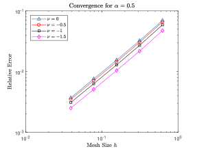
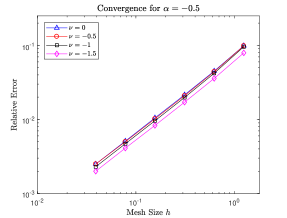
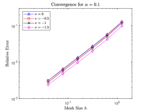
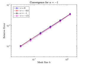
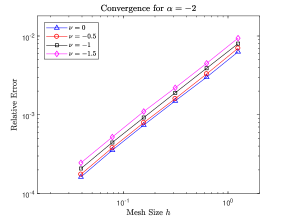
For each model configuration, we computed approximate solutions over a sequence of uniform meshes, refining at each step by halving the mesh parameter . The charts in Figure 1 plot the observed relative error against the mesh parameter , for all possible parameter configurations. From even the briefest examination of the charts it is clear that as the mesh is refined, the relative error of the approximations is reduced. Whilst if we were to examine the gradients of the lines appearing in Figure 1, then they appear generally to be getting closer to 1, as the mesh is refined. With the gradients between the most refined mesh pairings having a mean value of 1.0301, across all configurations. This would suggest that our numerical scheme has order , with the error in the approximations being . The full numerical details of the errors and the associated convergence rates underlying Figure 1 may be found in [27, Appendix A].
8. Conclusions
In this article we introduced a numerical scheme for the approximate solution of a truncated version of a mixed discrete-continuous fragmentation model. The scheme was based upon a finite volume discretisation of the modelling equation for the continuous component.
The resulting numerical approximations were first shown to be nonnegative and to conserve mass, provided the underlying mesh satisfied certain constraints. Following which we established the weak convergence of a subsequence of our approximations, as the mesh size parameter was decreased to zero. The resulting limits were then shown to provide a weak solution to the truncated model.
By relating the scalar-valued weak formulation of our truncated model to an equivalent weak formulation within a Banach space setting, we were able to establish a one-to-one relationship between any scalar and Banach-space-valued weak solutions. Under suitable constraints, these Banach-space-valued weak solutions were shown to provide the unique strong solution to the associated abstract Cauchy problem, in the process establishing the uniqueness of the original scalar-valued weak solutions. Additionally, as a further consequence of this linkage, the scalar weak solutions were shown to be differentiable classical solutions.
Finally, by conducting a range of experiments with a test model, under varying model parameter choices and mesh refinements, we experimentally established that the error in our numerical solutions was .
Acknowledgments
This work was supported by the UK Engineering and Physical Sciences Research Council [EP/J500495/1 03].
References
- [1] R. Ziff, Kinetics of polymerization, Journal of Statistical Physics 23 (2) (1980) 241–263.
- [2] M. Costas, M. Moreau, L. Vicente, Some analytical and numerical solutions for colloidal aggregation with fragmentation, Journal of Physics A: Mathematical and General 28 (11) (1995) 2981–2994.
- [3] P. Degond, J.-G. Liu, R. Pego, Coagulation–fragmentation model for animal group-size statistics, Journal of Nonlinear Science 27 (2) (2017) 379–424.
- [4] P. Degond, M. Engel, Numerical approximation of a coagulation–fragmentation model for animal group size statistics, Networks & Heterogeneous Media 12 (2) (2017) 217–243.
- [5] A. Johansen, F. Brauer, C. Dullemond, H. Klahr, A coagulation–fragmentation model for the turbulent growth and destruction of preplanetesimals, Astronomy & Astrophysics 486 (2) (2008) 597–611.
- [6] J. Drazkowska, F. Windmark, C. Dullemond, Modeling dust growth in protoplanetary disks: The breakthrough case, Astronomy & Astrophysics 567 (2014) A38.
- [7] F. Guias, A Monte Carlo approach to the Smoluchowski equations, Monte Carlo Methods and Applications 3 (1997) 313–326.
- [8] H. Babovsky, On a Monte Carlo approach to the Smoluchowski equations, Monte Carlo Methods and Applications 5 (1999) 1–18.
- [9] A. Eibeck, W. Wagner, An efficient stochastic algorithm for studying coagulation dynamics and gelation phenomena, SIAM Journal on Scientific Computing 22 (3) (2000) 802–821.
- [10] S. Kumar, D. Ramkrishna, On the solution of population balance equations by discretization–I. A fixed pivot technique, Chemical Engineering Science 51 (8) (1996) 1311–1332.
- [11] M. Nicmanis, M. Hounslow, A finite element analysis of the steady state population balance equation for particulate systems: Aggregation and growth, Computers & Chemical Engineering 20 (1996) S261–S266.
- [12] J. Barrett, J. Jheeta, Improving the accuracy of the moments method for solving the aerosol general dynamic equation, Journal of Aerosol Science 27 (8) (1996) 1135–1142.
- [13] A. Smirnov, S. Matveev, D. Dmitry A. Zheltkov, E. Tyrtyshnikov, Fast and accurate finite-difference method solving multicomponent Smoluchowski coagulation equation with source and sink terms, Procedia Computer Science 80 (2016) 2141–2146.
-
[14]
R. Kumar,
Numerical
analysis of finite volume schemes for population balance equations, Ph.D.
thesis, Otto-von-Guericke University Magdeburg (2010).
URL https://www.researchgate.net/publication/50870176_Numerical_analysis_for_finite_volume_schemes_for_population_balance_equations - [15] G. Baird, E. Süli, A mixed discrete–continuous fragmentation model, Journal of Mathematical Analysis and Applications 473 (1) (2019) 273–296.
- [16] E. McGrady, R. Ziff, Shattering transition in fragmentation, Phys. Rev. Lett. 58 (1987) 892–895.
- [17] F. Filbet, P. Laurençot, Numerical simulation of the Smoluchowski coagulation equation, SIAM Journal on Scientific Computing 25 (6) (2004) 2004–2028.
- [18] J. Bourgade, F. Filbet, Convergence of a finite volume scheme for coagulation–fragmentation equations, Math. Comp. 77 (2008) 851–882.
- [19] J. Kumar, J. Saha, E. Tsotsas, Development and convergence analysis of a finite volume scheme for solving breakage equation, SIAM Journal on Numerical Analysis 53 (4) (2015) 1672–1689.
- [20] R. Kumar, J. Kumar, G. Warnecke, Convergence analysis of a finite volume scheme for solving non-linear aggregation-breakage population balance equations, Kinetic & Related Models 7 (2014) 713–737.
- [21] F. Filbet, An asymptotically stable scheme for diffusive coagulation–fragmentation models, Communications in Mathematical Sciences 6 (2) (2008) 257–280.
- [22] S. Qamar, G. Warnecke, M. Elsner, On the solution of population balances for nucleation, growth, aggregation and breakage processes, Chemical Engineering Science 64 (9) (2009) 2088–2095.
- [23] R. Kumar, J. Kumar, G. Warnecke, Moment preserving finite volume schemes for solving population balance equations incorporating aggregation, breakage, growth and source terms, Mathematical Models and Methods in Applied Sciences 23 (07) (2013) 1235–1273.
- [24] S. Qamar, G. Gerald Warnecke, Solving population balance equations for two-component aggregation by a finite volume scheme, Chemical Engineering Science 62 (3) (2007) 679–693.
- [25] L. Forestier-Coste, S. Mancini, A finite volume preserving scheme on nonuniform meshes and for multidimensional coalescence, SIAM Journal on Scientific Computing 34 (6) (2012) B840–B860.
- [26] J. Saha, N. Das, J. Kumar, A. Bück, Numerical solutions for multidimensional fragmentation problems using finite volume methods, Kinetic & Related Models 12 (2019) 79–103.
-
[27]
G. Baird,
Mixed
discrete–continuous fragmentation equations, Ph.D. thesis, University of
Oxford (2017).
URL https://ora.ox.ac.uk/objects/uuid:311da0da-6801-4120-9129-d95786a153b6 - [28] D. McLaughlin, W. Lamb, A. McBride, A semigroup approach to fragmentation models, SIAM J. Math. Anal. 28 (1997) 1158–1172.
- [29] I. Stewart, E. Meister, A global existence theorem for the general coagulation–fragmentation equation with unbounded kernels, Mathematical Methods in the Applied Sciences 11 (5) (1989) 627–648.
- [30] J. Banasiak, L. Arlotti, Perturbations of Positive Semigroups with Applications, Springer-Verlag, London, 2006.
- [31] I. Fonseca, G. Leoni, Modern Methods in the Calculus of Variations: Spaces, Springer New York, 2007.
- [32] P. Laurençot, Weak compactness techniques and coagulation equations, in: Evolutionary equations with applications in natural sciences, Vol. 2126 of Lecture Notes in Math., Springer International Publishing, 2015, pp. 199–253.
- [33] E. Lieb, M. Loss, Analysis, Graduate Studies in Mathematics, American Mathematical Society, 2001.
- [34] K. Engel, R. Nagel, One-Parameter Semigroups for Linear Evolution Equations, Springer, New York, 2000.
- [35] A. Pazy, Semigroups of Linear Operators and Applications to Partial Differential Equations, Springer, New York, 1983.
- [36] A. Belleni-Morante, A. McBride, Applied Nonlinear Semigroups, Wiley, Chichester, 1998.
- [37] W. Arendt, C. Batty, M. Hieber, F. Neubrander, Vector-Valued Laplace Transforms and Cauchy Problems, Monographs in mathematics, Birkhauser Verlag, 2001.
-
[38]
J. Canizo, Evolution equations in a
Banach space (2006).
URL http://canizo.org/tex/evolution.pdf - [39] J. Diestel, J. Uhl, Vector Measures, Mathematical surveys and monographs, American Mathematical Society, 1977.