Optimal common resource in majorization-based resource theories

We address the problem of finding the optimal common resource for an arbitrary family of target states in quantum resource theories based on majorization, that is, theories whose conversion law between resources is determined by a majorization relationship, such as it happens with entanglement, coherence or purity. We provide a conclusive answer to this problem by appealing to the completeness property of the majorization lattice. We give a proof of this property that relies heavily on the more geometric construction provided by the Lorenz curves, which allows to explicitly obtain the corresponding infimum and supremum. Our framework includes the case of possibly non-denumerable sets of target states (i.e., targets sets described by continuous parameters). In addition, we show that a notion of approximate majorization, which has recently found application in quantum thermodynamics, is in close relation with the completeness of this lattice. Finally, we provide some examples of optimal common resources within the resource theory of quantum coherence.

Keywords: quantum resource theories, majorization lattice, optimal common resource

1 Introduction

Quantum resource theories (QRTs) are a very general and powerful framework for studying different phenomena in quantum theory from an operational point of view (see Ref. [1] for a recent review of the topic). Indeed, all QRTs are built from three basics components: free states, free operations and resources. These components are not independent among each other, and they are defined in a way that depends on the physical properties that one wants to describe. In general, for a given QRT, one defines the set of free sates $\mathcal{F}$, formed by those states that can be generated without too much effort. Then, an operation $\mathcal{E}$ is said to be free, if it satisfies the condition of mapping free states into free states: $\mathcal{E}$ is free if and only if $\mathcal{E}(\rho)\in\mathcal{F}\ \forall\ \rho\in\mathcal{F}$. Thus, free operations can be interpreted as the ones that are easy to implement in the lab. Finally, quantum resources are defined as those states that do not belong to the set of free states (i.e., $\rho\notin\mathcal{F}$). These states are the useful ones for doing the corresponding quantum tasks. As an illustration, consider the task of transmitting an arbitrary quantum state from one lab to another distant one, where the allowed free operations are the so-called local operations and classical communication (LOCC). In this typical scenario, entanglement arises as the necessary quantum resource to perform this task (as it can be seen from the quantum teleportation protocol [2]).

Clearly, it is not possible to convert free states into resources by appealing to free operations alone. This is the reason why the term resource theory was coined. In fact, one of the main concerns of the QRTs is the characterization of transformations between resources by means of free operations. Here, we are focused on QRTs for which these transformations are fully characterized by a kind of majorization law between the resources. Precisely, we are interested in QRTs for which $\rho\underset{\mathrm{free}}{\rightarrow}\sigma$ is equivalent to $x(\rho)\succeq x(\sigma)$ or $x(\sigma)\succeq x(\rho)$, where $x(\rho)$ and $x(\sigma)$ are probability vectors associated to $\rho$ and $\sigma$, respectively, and $\succeq$ means a majorization relation (see e.g.  [3] for an introduction to majorization theory). In addition to the characterization of the convertibility of free states by means of free operations [4, 5, 6, 7, 8, 9, 10], majorization theory has been applied to different problems in quantum information such as entanglement criteria [11, 12], majorization uncertainty relations [14, 13, 15, 16, 17], quantum entropies [18, 19, 20] and quantum algorithms [21], among others [22, 23, 24, 25, 26].

We restrict to QRTs based on majorization mainly for two reasons. As we have already mentioned, there are several examples of QRTs that satisfy a majorization law (see Table 1 and Refs. [4, 5, 6, 7, 8, 9, 10]). Thus, the results obtained which are based in the properties of majorization are of great generality, providing a unifying framework for several physical problems. On the other hand, majorization induces a lattice structure [27, 28, 29]. We will show that this allows to introduce the notion of optimal common resource in a very natural way. Before doing that, we stress that the lattice theoretical aspects of majorization theory have not been sufficiently exploited in comparison with other features of it in the area of quantum information. Indeed, the first applications were given in Refs. [30, 31]; only recently, new applications of the majorization lattice have been found [32, 33, 34, 35, 36, 37, 38, 39].

QRT	Free operations	Resources	Probability vector
Entanglement (pure) [4]	LOCC	$\ket{\psi}=\sum_{i}\sqrt{\psi_{i}}\ket{i^{A}}\ket{i^{B}}\in\mathbb{C}^{d_{A}}\otimes\mathbb{C}^{d_{B}}$ (Schmidt decomposition)	$x(\psi)\equiv[\psi_{1},\ldots,\psi_{d}]$ with $d=\min\{d_{A},d_{B}\}$
Coherence (pure) [5, 6, 7, 8]	IO	$\ket{\psi}=\sum_{i}\psi_{i}\ket{i}\in\mathbb{C}^{d}$ ($\{\ket{i}\}$ incoherent basis)	$x(\psi)\equiv[|\psi|^{2}_{1},\ldots,|\psi|^{2}_{d}]$
Purity [9, 10]	Unital	$\rho\neq\frac{I}{d}$ acting on $\mathbb{C}^{d}$	$x(\rho)\equiv[\rho_{1},\ldots,\rho_{d}]$ with $\rho_{i}$ eigenvalues of $\rho$

Table 1: Quantum resource theories where the transformations between resources by means of free operations are given by a majorization relation. For each QRT, the corresponding free operations are: local operations and classical communication (LOCC), incoherent operations (IO) and unital, respectively.

Here, we aim to address the following problem. Let us suppose that one wants to have a set of target resources $\mathcal{T}$. For obvious practical reasons, it is very useful to find a resource $\rho$, such that it can be converted by means of free operations to any other resource belonging to the target set, that is, $\rho\underset{\mathrm{free}}{\rightarrow}\sigma$ for all $\sigma\in\mathcal{T}$. By definition, the maximal resource (if it exists) has to perform this task for any target set in a given QRT. But a more interesting question is whether there exists a state that can carry out the same task, but using the least amount of resources as possible. More precisely, one aims to find a resource $\rho^{\mathrm{ocr}}$ such that $\rho^{\mathrm{ocr}}\underset{\mathrm{free}}{\rightarrow}\sigma\ \forall\sigma\in\mathcal{T}$, and for any other $\rho$ satisfying $\rho\underset{\mathrm{free}}{\rightarrow}\sigma\ \forall\sigma\in\mathcal{T}$, then either $\rho\underset{\mathrm{free}}{\rightarrow}\rho^{\mathrm{ocr}}$ or $\rho\underset{\mathrm{free}}{\nleftrightarrow}\rho^{\mathrm{ocr}}$. If this state exists, we refer to it as the optimal common resource (ocr). In this work, we provide a solution for the problem of finding the optimal common resources for arbitrary target sets of all QRTs based on majorization. This problem was already posed and (partially) solved in Ref. [37], for possibly infinite (but denumerable) target sets of bipartite pure entangled states. Let us stress that our proposal is a twofold extension of that previous work. In the first place, we provide a unifying framework for arbitrary QRTs based on majorization, which includes not only entanglement resource theory, but also the important cases of coherence and purity resource theories. In the second place, we consider the most general case of possibly non-denumerable sets of target resources. This is a powerful extension of previous works, because it allows to apply this technique to target sets which are described by a continuous family of parameters. We provide the answer to this general problem by appealing to the completeness of the majorization lattice [27, 28]. In particular, our construction relies on the geometrical properties of Lorenz curves associated to the corresponding target set of probability vectors, which allow us to provide an explicit algorithm for the computation not only of the infimum (as in [27]) but also of the supremum. We also describe, for convex polytopes, the relationship between the infimum and supremum and their extreme points.

2 Majorization lattice

Here, we introduce the majorization lattice and present its most salient order-theoretic features.

Let us consider probability vectors whose entries are sorted in non-increasing order, that is, vectors belonging to the set:

$$\Delta_{d}^{\downarrow}\equiv\left\{\left[x_{1},\ldots,x_{d}\right]:x_{i}\geq x_{i+1}\geq 0\ \mbox{and}\ \sum_{i=1}^{d}x_{i}=1\right\}.$$ (1)

Geometrically, this set is a convex polytope embedded in the $d-1$-probability simplex.

Let us now introduce the notion of majorization between probability vectors (see, e.g. [3]).

Definition 1.

For given $x,y\in\Delta_{d}^{\downarrow}$, it is said that $x$ majorizes $y$, denoted as $x\succeq y$, if and only if,

$$\sum_{i=1}^{k}x_{i}\geq\sum_{i=1}^{k}y_{i}\ \forall\,k=1,\ldots,d-1.$$ (2)

Notice that $\sum_{i=1}^{d}x_{k}=\sum_{i=1}^{d}y_{k}$ is trivially satisfied, because $x$ and $y$ are probability vectors (so we can discard this condition from the definition of majorization).

The intuitive idea of majorization is that a probability distribution majorizes another one, whenever the former is more concentrated than the latter. In this sense, majorization provides a quantification of the notion of non-uniformity. To fix ideas, let us observe that any probability vector $x\in\Delta_{d}^{\downarrow}$ trivially satisfies the majorization relations: $e_{d}\equiv[1,0,\dots,0]\succeq x\succeq\left[\frac{1}{\mathrm{rank}x},\ldots,\frac{1}{\mathrm{rank}x},0,\ldots,0\right]\succeq\left[\frac{1}{d},\ldots,\frac{1}{d}\right]\equiv u_{d}$, where $\mathrm{rank}x$ is the number of positives entries of $x$, and $e_{d}$ and $u_{d}$ are the extreme $d$-dimensional probability vectors in the sense of maximum non-uniformity ($e_{d}$) and minimum non-uniformity ($u_{d}$, i.e. the uniform probability vector), respectively. Let us remark that there are several equivalent definitions of majorization that connect it with the notions of double stochastic matrices, Schur-concave functions and entropies, among others (see e.g. [3]).

Here we are interested in the order-theoretic properties of majorization. Indeed, it can be shown that the set $\Delta_{d}^{\downarrow}$ together with the majorization relation is a partially ordered set (POSET, see e.g.  [40] for an introduction to order theory). This means that that, for every $x,y,z\in\Delta_{d}^{\downarrow}$ one has

1. reflexivity: $x\succeq x$,

2. antisymmetry: $x\succeq y$ and $y\succeq x$, then $x=y$, and

3. transitivity: $x\succeq y$ and $y\succeq z$, then $x\succeq z$.

Notice that if one leaves the constraint that the entries of the probability vectors are sorted in non-increasing order, then condition (ii) is not valid in general. Instead of this, a weaker version holds, where $x$ and $y$ differ only by a permutation of its entries. In such case, majorization gives a preorder because condition (i) and (iii) remain valid.

In general, majorization does not yields a total order for probability vectors belonging to $\Delta_{d}^{\downarrow}$. This is because there exist $x,y\in\Delta_{d}^{\downarrow}$ such that $x\nsucceq y$ and $y\nsucceq x$ for any $d>2$. In this situation, we say that the probability vectors are incomparable. For instance, it is straightforward to check that $x=[0.6,0.16,0.16,0.08]$ and $y=[0.5,0.3,0.1,0.1]$ are incomparable.

There is a visual way to address majorization that consists in appealing to the notion of Lorenz curve [41]. More precisely, for a given $x\in\Delta_{d}^{\downarrow}$ one introduces the set of points $\left\{(k,\sum_{i=1}^{k}x_{i})\right\}_{k=0}^{d}$ (with the convention $(0,0)$ for $k=0$). Then, the Lorenz curve of $x$, say $L_{x}(\omega)$ with $\omega\in[0,d]$, is obtained by the linear interpolation of these points. At the end, one obtains a non-decreasing and concave polygonal curve from $(0,0)$ to $(d,1)$. In this way, given two Lorenz curves of $x$ and $y$, if the Lorenz curve of $x$ is greater (or equal) than the one of $y$, it implies that $x$ majorizes $y$, and vice versa. On the other hand, if two different Lorenz curves intersect at least at one point in the interval $(1,d)$, it means that $x$ and $y$ are incomparable. See for example Fig. 1, where the Lorenz curve of $e_{4},u_{4},x=[0.6,0.16,0.16,0.08]$ and $y=[0.5,0.3,0.1,0.1]$ are plotted. It is clear that $e_{4}\succeq x\succeq u_{4}$ and $e_{4}\succeq y\succeq u_{4}$, but $x\nsucceq y$ and $y\nsucceq x$. However, in such case, one can easily realize that there are infinite Lorenz curves below the ones of $x$ and $y$, and among of all them, there is one which is the greatest one. In the same vein, there are infinitely many Lorenz curves above those of $x$ and $y$, and there is one which is the lowest one.

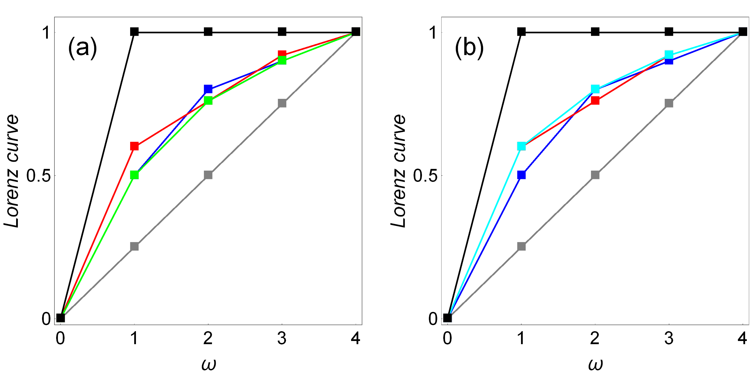
Figure 1: Lorenz curves of of $e_{4}$ (black), $u_{4}$ (gray), $x=[0.6,0.16,0.16,0.08]$ (red) and $y=[0.5,0.3,0.1,0.1]$ (blue). (a) Among all Lorenz curves below the ones of $x$ and $y$, there exists the greatest Lorenz curve that corresponds to the probability vector $x\wedge y=[0.5,0.26,0.14,0.1]$ (green). (b) Among all Lorenz curves above the ones of $x$ and $y$, there exists the lowest Lorenz curve that corresponds to the probability vector $x\vee y=[0.6,0.2,0.12,0.08]$ (cyan).

These intuitions can be formalized and allow to formulate a notion of infimum and supremum in the general case [29, 27, 28]. Consequently, the definition of majorization lattice is introduced as follows:

Definition 2.

The quadruple $\mathcal{L}=\langle\Delta_{d}^{\downarrow},\succeq,e_{d},u_{d}\rangle$ defines a bounded lattice order structure, where $e_{d}=[1,0,\ldots,0]$ is the top element, $u_{d}=\left[\frac{1}{d},\ldots,\frac{1}{d}\right]$ is the bottom element and for all $x,y\in\Delta_{d}^{\downarrow}$ the infimum $x\wedge y$ and the supremum $x\vee y$ are expressed as in [29] (or see below).

Precisely, the components of the infimum are given by iteration of the formula

$$(x\wedge y)_{k}=\min\left\{\sum^{k}_{i=1}x_{i},\sum^{k}_{i=1}y_{i}\right\}-\min\left\{\sum^{k-1}_{i=1}x_{i},\sum^{k-1}_{i=1}y_{i}\right\},$$ (3)

for $k=1,\ldots,d$ and the convention that summations with the upper index smaller than the lower index are equal to zero. For the supremum, one has to proceed in two steps. First, one has to calculate the probability vector, say $z$, with components given by

$$z_{k}=\max\left\{\sum^{k}_{i=1}x_{i},\sum^{k}_{i=1}y_{i}\right\}-\max\left\{\sum^{k-1}_{i=1}x_{i},\sum^{k-1}_{i=1}y_{i}\right\}.$$ (4)

In general, this vector does not belong to $\Delta_{d}^{\downarrow}$, because its components are not in a decreasing order. If it is the case that $z\in\Delta_{d}^{\downarrow}$, then $z=x\vee y$. Otherwise, one has to apply the flatness process (see [29, Lemma 3]) in order to get the supremum, as follows. For a probability vector $w=[w_{1},\ldots,w_{d}]^{t}$, let $j$ be the smallest integer in $[2,d]$ such that $w_{j}>w_{j-1}$ and let $k$ be the greatest integer in $[1,j-1]$ such that

$$w_{k-1}\geq\frac{\sum_{l=k}^{j}w_{l}}{j-k+1}=a,$$ (5)

with $w_{0}>1$. Then, a flatness probability vector $w^{\prime}$ is given by

$$w^{\prime}_{l}=\left\{\begin{array}[]{cc}a&\mbox{for}\ l=k,k+1,\ldots,j\\ w_{l}&\mbox{otherwise}.\end{array}\right.$$ (6)

Then, the supremum is obtained in no more than $d-1$ iterations, by iteratively applying the above transformations with the input probability vector $z$ given by (4), until one obtains a probability vector in $\Delta_{d}^{\downarrow}$.

Let us consider a finite set of probability vectors, that is, $\mathcal{P}=\{x^{1},\ldots,x^{N}\}$ with $\ x^{i}\in\Delta_{d}^{\downarrow}$. By appealing to the algebraic properties of the definition of lattice, it is straightforward to show that the infimum and the supremum of $\mathcal{P}$ always exist, and are given by $\bigwedge\mathcal{P}=x^{1}\wedge x^{2}\wedge\ldots\wedge x^{N}$ and $\bigvee\mathcal{P}=x^{1}\vee x^{2}\vee\ldots\vee x^{N}$. However, if one considers an arbitrary set of probability vectors (which could be infinite), the lattice properties are not strong enough to guarantee the existence of infimum and supremum. If the infimum and supremum exist for arbitrary families, the lattice is said to be complete. It has been shown that the majorization lattice is indeed complete [27, 28]. For the sake of completeness, we reproduce the demonstration here and extend it in the following sense: we provide an explicit algorithm for computing the supremum.

Proposition 1.

Let $\mathcal{P}$ an arbitrary set of probability vectors such that $\mathcal{P}\subseteq\Delta_{d}^{\downarrow}$. Then, there exist the infimum $x^{\inf}\equiv\bigwedge\mathcal{P}$ and the supremum $x^{\sup}\equiv\bigvee\mathcal{P}$ of $\mathcal{P}$.

In addition, the components of the $x^{\inf}$ are given by

$$x^{\inf}_{k}=\inf\left\{\mathcal{S}_{k}\right\}-\inf\left\{\mathcal{S}_{k-1}\right\},$$ (7)

where $\mathcal{S}_{k}=\{S_{k}(x):x\in\mathcal{P}\}$ with $S_{k}(x)\equiv\sum^{k}_{i=1}x_{i}$ for $k\in\{1,\ldots,d\}$ and $S_{0}(x)\equiv 0$.

On the other hand, to obtain the components of the $x^{\sup}$, we have first to define the probability vector with components given by

$$\bar{x}_{k}=\sup\left\{\mathcal{S}_{k}\right\}-\sup\left\{\mathcal{S}_{k-1}\right\}.$$ (8)

Then, we compute the upper envelope of the polygonal given by the linear interpolation of the points $\{(k,S_{k}(\bar{x}))\}_{k=0}^{d}$, say $\bar{L}(\omega)$, by using the algorithm 1. Finally, the components of the supremum are given by:

$$x^{\sup}_{k}=\bar{L}(k)-\bar{L}(k-1).$$ (9)

The proof of Proposition 1 is given in A.1. Clearly, when the set is given by two probability vectors in $\Delta_{d}^{\downarrow}$, that is $\mathcal{P}=\{x,y\}$, the calculus of infimum and supremum of the Proposition 1 reduces to the procedure given in Ref. [29] (see Eqs. (3)–(6)).

Infimum and supremum over convex polytopes

Let us illustrate the meaning and relevance of the infimum and supremum discussed above with an interesting example. First, let us note that if $\mathcal{P}\subseteq\Delta_{d}^{\downarrow}$ is a convex polytope, then the corresponding infimum and supremum can be computed as the infimum and supremum of the set of vertices, $\mathrm{vert}(\mathcal{P})$.

Lemma 1.

Let $\mathcal{P}$ be a convex polytope contained in $\Delta_{d}^{\downarrow}$, and $\mathrm{vert}(\mathcal{P})$ the set of vertices, $\mathrm{vert}(\mathcal{P})=\{v^{n}\}^{N}_{n=1}$. Then, the infimum $x^{\inf}\equiv\bigwedge\mathcal{P}$ and the supremum $x^{\sup}\equiv\bigvee\mathcal{P}$ of $\mathcal{P}$ are given by the infimum and supremum elements of $\mathrm{vert}(\mathcal{P})$, namely

$$x^{\inf}=\bigwedge\{v^{n}\}^{N}_{n=1}\quad\mbox{and}\quad x^{\sup}=\bigvee\{v^{n}\}^{N}_{n=1}.$$ (10)

The proof of Lemma 1 is given in A.2. Notice that, although the problem is reduced to the calculation of the infimum and supremum among the extreme points of the convex polytope, $x^{\inf}$ and $x^{\sup}$ do not necessarily belong to it (see e.g. , Fig. 2.(a)). However, we will see an interesting example where the infimum and supremum do belong to the given convex polytope (see e.g. , Fig. 2.(b)).

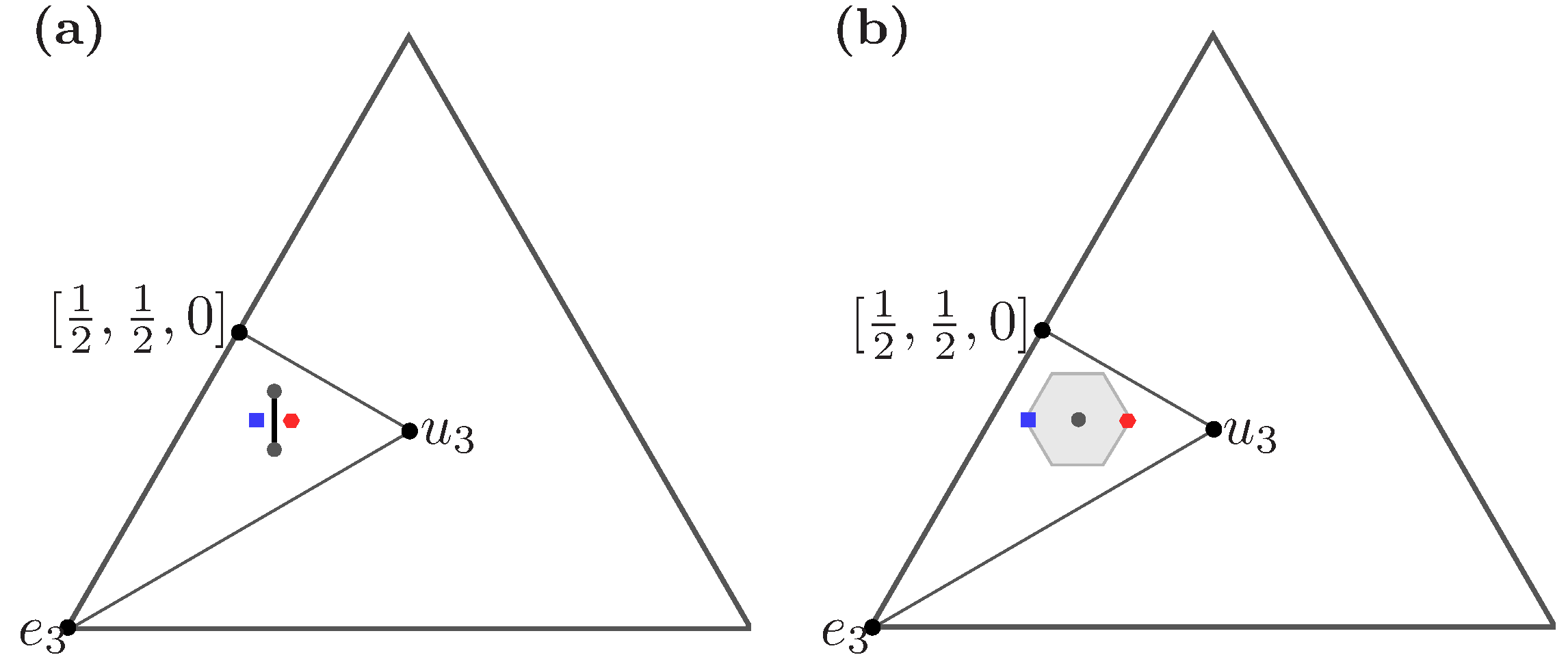
Figure 2: Infimum and supremum of convex polytopes in $\Delta^{\downarrow}_{3}$ (region formed by the convex hull of $e_{3}$, $u_{3}$ and $\left[\frac{1}{2},\frac{1}{2},0\right]$) for (a) $\mathcal{P}=\left\{x\in\Delta^{\downarrow}_{3}:x=p[0.5,0.4,0.1]+(1-p)[0.55,0.3,0.15]\,\mbox{with}\,p\in[0,1]\right\}$ (black line), where $\bigwedge\mathcal{P}=[0.5,0.35,0.15]$ (red hexagon) and $\bigvee\mathcal{P}=[0.55,0.35,0.1]$ (blue square); and (b) $\mathcal{P}=B_{0.15}([0.525,0.35,0.125])$ (light gray region), where $\bigwedge\mathcal{P}=[0.45,0.35,0.2]$ (red hexagon) and $\bigvee\mathcal{P}=[0.6,0.35,0.05]$ (blue square).

Let us consider the $\ell_{1}$–norm $\epsilon$–ball centered in $x^{0}\in\Delta_{d}^{\downarrow}$ intersected with $\Delta_{d}^{\downarrow}$, that is, $B_{\epsilon}(x^{0})=\{x^{\prime}\in\Delta_{d}^{\downarrow}:||x^{\prime}-x^{0}||_{1}\leq\epsilon\}$, where $||x||_{1}\equiv\sum^{d}_{i=1}|x_{i}|$ denotes the $\ell_{1}$–norm of a probability vector. Let us first note that $\{x^{\prime}\in\mathbb{R}^{d}:||x^{\prime}-x^{0}||_{1}\leq\epsilon\}$ is a convex polytope (see Ref. [20]). Then, $B_{\epsilon}(x^{0})$ is also a convex polytope, because it is the intersection of that convex polytope with $\Delta_{d}^{\downarrow}$. Therefore, by applying Lemma 1, $\bigwedge B_{\epsilon}(x^{0})$ and $\bigvee B_{\epsilon}(x^{0})$ reduces to finding the infimum and supremum of the vertices of $B_{\epsilon}(x^{0})$.

Interestingly enough, the lattice-theoretic property of majorization can be posed in strong connection with the notion of approximate majorization [20, 42], which has recently found application in quantum thermodynamics [43]. More precisely, the steepest $\epsilon$-approximation, $\bar{x}^{0(\epsilon)}\in B_{\epsilon}(x^{0})$, and the flattest $\epsilon$-approximation, $\underline{x}^{0(\epsilon)}\in B_{\epsilon}(x^{0})$, of $x^{0}$ given in [20, 42] satisfy that, $\bar{x}^{0(\epsilon)}\succeq x\succeq\underline{x}^{0(\epsilon)}$ for all $x\in B_{\epsilon}(x^{0})$. Using the definition of infimum and supremum of a given family, it follows that $\bar{x}^{0(\epsilon)}=x^{\sup}$ and $\underline{x}^{0(\epsilon)}=x^{\inf}$, although the algorithms to obtain them are different to the ones presented here. Thus, we see that the notion of approximate majorization is in strong connection with the property of completeness of the majorization lattice. Furthermore, we have shown that it can be reduced to the application of the algorithm of infimum and supremum to the set of vertices of $B_{\epsilon}(x^{0})$.

3 Optimal common resource

Now, we are ready to apply the Proposition 1 to the problem of finding the optimal common resource in QRTs based on majorization.

In the first place, we have to distinguish between two possible cases of QRTs based on majorization. We call direct majorization-based QRTs to those QRTs such that $\rho\underset{\mathrm{free}}{\rightarrow}\sigma$ iff $x(\rho)\succeq x(\sigma)$, whereas we call reversed majorization-based QRTs to those that reverse the majorization relation (that is, $\rho\underset{\mathrm{free}}{\rightarrow}\sigma$ iff $x(\sigma)\succeq x(\rho)$). Notice that purity is of the former type, whereas entanglement and coherence are of the latter one (see Table 1). For such QRTs, let us remark that $\rho^{\mathrm{ocr}}$ is an optimal common resource if $\rho^{\mathrm{ocr}}\underset{\mathrm{free}}{\rightarrow}\sigma\ \forall\sigma\in\mathcal{T}$, and for any other $\rho$ satisfying $\rho\underset{\mathrm{free}}{\rightarrow}\sigma\ \forall\sigma\in\mathcal{T}$ one has $\rho\underset{\mathrm{free}}{\rightarrow}\rho^{\mathrm{ocr}}$. Let us observe that all states $\rho$ such that $\rho^{\mathrm{ocr}}\underset{\mathrm{free}}{\leftrightarrow}\rho$ are equivalent in the sense that all of them are optimal common resources.

For a given set of target resources $\mathcal{T}$, let us consider its corresponding set of probability vectors $\mathcal{P}$, which depends on the majorization-based QRT that one is dealing with. We show now that the problem of finding an optimal common resource within a QRT based on majorization, can be reduced to an application of the completeness of the majorization lattice. Indeed, by directly applying Proposition 1, one finds that an optimal common resource of $\mathcal{T}$ for direct majorization-based QRTs can be obtained from the supremum of the corresponding set of probability vectors $\mathcal{P}$. On the other hand, for reversed majorization-based QRTs, it can be obtained from the infimum of the corresponding set of probability vectors $\mathcal{P}$.

In this way, the completeness of the majorization lattice is of the essence in dealing with the optimal common resources in QRTs based on majorization. As we have already stressed in the Introduction, this is a twofold extension of the proposal of Ref. [37].

Optimal common resource within the resource theory of quantum coherence

In the following, we illustrate how to obtain an optimal common resource within the resource theory of quantum coherence introduced in Ref. [46].

Deterministic transformations between pure sates by means of incoherent operations (free operations) have been addressed in several works [5, 6, 7, 8]. In particular, we consider two pure sates $\ket{\psi}=\sum_{i=1}^{d}\psi_{i}\ket{i}$ and $\ket{\phi}=\sum_{i=1}^{d}\phi_{i}\ket{i}$, where $\{\ket{i}\}_{i=1}^{d}$ is a fixed orthonormal basis (the incoherent basis) of a $d$-dimensional Hilbert space. The coefficients $\{\psi_{i}\}$ and $\{\phi_{i}\}$ are complex numbers in general, satisfying $\sum_{i=1}^{d}|\psi_{i}|^{2}=\sum_{i=1}^{d}|\phi_{i}|^{2}=1$. Let $x(\psi)$ and $x(\phi)$ be the probability vectors in $\Delta_{d}^{\downarrow}$ associated to these pure states, that is, $x_{i}(\psi)=|\psi_{[i]}|^{2}$ and $x_{i}(\phi)=|\phi_{[i]}|^{2}$, where $|\psi_{[i+1]}|\geq|\psi_{[i]}|$ and $|\phi_{[i+1]}|\geq|\phi_{[i]}|$ for all $i$. It has be shown that $\ket{\psi}$ can be converted into $\ket{\phi}$ by means of incoherent operations (IO), denoted as $\ket{\psi}\underset{\mathrm{IO}}{\rightarrow}\ket{\phi}$, if and only if $x(\phi)\succeq x(\psi)$ (see e.g. Ref. [47] and references therein). This result can be seen as the analog of the celebrated Nielsen’s theorem [4] for quantum coherence.

Let us recall that $\sum_{i=1}^{d}\frac{1}{\sqrt{d}}\ket{i}$ is a maximally coherent state, since it can be converted into any other state by means of incoherent operations [46]. We are going to discuss two cases in which the optimal common resource is not a maximally coherent one.

As a first example, if we consider a subset of pure states given by $\mathcal{T}=\left\{\ket{\phi}\in\mathbb{C}^{d}:|\phi_{[1]}|\geq\alpha\right\}$ with $1/\sqrt{d}<\alpha\leq 1$, to find an optimal common resource of $\mathcal{T}$ we have to calculate the infimum of the set $\mathcal{P}=\{x\in\Delta_{d}^{\downarrow}:x_{1}\geq\alpha^{2}\}$. It can be shown that $\bigwedge\mathcal{P}=\left[\alpha^{2},\frac{1-\alpha^{2}}{d-1},\ldots,\frac{1-\alpha^{2}}{d-1}\right]$, so that an optimal common resource has the form $\ket{\psi^{\mathrm{ocr}}}=\alpha\ket{1}+\sum_{i=2}^{d}\sqrt{\frac{1-\alpha^{2}}{d-1}}\ket{i}$. Clearly this optimal common resource is not a maximally coherent state.

As a second example, motivated by the study of coherence of quantum superpositions [48], let us consider a more subtle target set formed by superpositions of given two orthogonal states. More precisely, let $\mathcal{T}=\left\{\ket{\phi}\in\mathbb{C}^{d}:\ket{\phi}=\alpha\ket{\mu}+\beta\ket{\nu}\right\}$, where $\ket{\mu}=\sum_{i=1}^{d_{1}}\frac{1}{\sqrt{d_{1}}}\ket{i}$, $\ket{\nu}=\sum_{i=d_{1}+1}^{d}\frac{1}{\sqrt{d-d_{1}}}\ket{i}$ and $\alpha^{2}+\beta^{2}=1$ (with $\alpha,\beta\in\mathbb{R}$ for simplicity). If we do not impose any other restriction over $\alpha$, then $\mathcal{T}$ contains the maximally coherent state, which is trivially the optimal common resource. In order to exclude that possibility, let us consider that $\alpha^{2}\neq d_{1}/d$. In particular, let us suppose that $\alpha^{2}>d_{1}/d$, so that there is $\alpha^{2}_{\min}$ such that $\alpha^{2}_{\min}\leq\alpha^{2}\leq 1$, with $\alpha^{2}_{\min}$ strictly greater than $d_{1}/d$ (the other case, with $\alpha^{2}<d_{1}/d$, is completely analogous). The corresponding set of probability vectors is

$$\mathcal{P}=\bigg{\{}x\in\Delta_{d}^{\downarrow}:x=\Big{[}\overbrace{\frac{\alpha^{2}}{d_{1}},\ldots,\frac{\alpha^{2}}{d_{1}}}^{d_{1}},\frac{1-\alpha^{2}}{d-d_{1}},\ldots,\frac{1-\alpha^{2}}{d-d_{1}}\Big{]}\bigg{\}},$$

and the infimum of $\Delta_{d}^{\downarrow}$ is shown to be

$$\bigwedge\mathcal{P}=\Big{[}\overbrace{\frac{\alpha^{2}_{\min}}{d_{1}},\ldots,\frac{\alpha^{2}_{\min}}{d_{1}}}^{d_{1}},\frac{1-\alpha^{2}_{\min}}{d-d_{1}},\ldots,\frac{1-\alpha^{2}_{\min}}{d-d_{1}}\Big{]}.$$

Therefore, an optimal common resource of $\mathcal{T}$ is of the form

$$\ket{\psi^{\mathrm{ocr}}}=\sum_{i=1}^{d_{1}}\sqrt{\frac{\alpha^{2}_{\min}}{d_{1}}}\ket{i}+\sum_{i=d_{1}+1}^{d}\sqrt{\frac{1-\alpha^{2}_{\min}}{d-d_{1}}}\ket{i}.$$

Notice that in this example $\ket{\psi^{\mathrm{ocr}}}\notin\mathcal{T}$.

4 Concluding remarks

In this paper we gave a solution for the problem of finding an optimal common resource for an arbitrary family of target states of a given a QRT based on majorization like entanglement, coherence or purity (see Table 1). Our method relies on the completeness properties of the majorization lattice. We provided concrete algorithms for computing the infimum and supremum of an arbitrary family of states (Proposition 1). Our contribution improves previous works (e.g. [27, 28, 29, 37]), in the sense that our algorithm works for target sets of arbitrary cardinality (i.e., we provide an expression for the supremum for possibly non-denumerable families of states). Also, for convex polytopes, we include a study of the relationship between the infimum and supremum, and their extreme points (Lemma 1).

In addition, we showed that the notion of approximate majorization is in strong connection with the property of completeness of the majorization lattice [20, 42]. Indeed, the flattest and steepest approximations are nothing more than the infimum and supremum of the corresponding set, respectively, and they can be calculated only from their vertices.

Finally, the fact that completeness of the majorization lattice is of the essence in dealing with the optimal common resources is illustrated with some examples within the resource theory of quantum coherence [46].

Appendix

A.1 Proof of Proposition 1

For the sake of completeness, we show here that the majorization lattice is complete. We stress that this has been proved in previous works [27, 28]. However, we give an alternative proof that relies heavily on the more geometric construction provided by the Lorenz curves. This allow us to provide an explicit algorithm for the computation not only of the infimum but also of the supremum (Proposition 1).

Let us first introduce some notations and definitions. Let us define the partial sum of the first $k$ components of a given vector $x$ as $S_{k}(x)\equiv\sum^{k}_{i=1}x_{i}$ with the convention $S_{0}(x)\equiv 0$. Now, let us consider the set formed by all partial sums up to $k$ that come from probability vectors in $\mathcal{P}$, that is, $\mathcal{S}_{k}=\{S_{k}(x)\,:\,x\in\mathcal{P}\}$ and its infimum $\underaccent{\bar}{S}_{k}\equiv\inf\mathcal{S}_{k}$ and supremum $\bar{S}_{k}\equiv\sup\mathcal{S}_{k}$. Notice that, for each $k=0,\ldots d$, both $\underaccent{\bar}{S}_{k}$ and $\bar{S}_{k}$ exist, since each $\mathcal{S}_{k}$ is a set of real numbers bounded from below by $\frac{k}{d}$ and above by $1$. Finally, let us consider the probability vectors $\underaccent{\bar}{x}=[\underaccent{\bar}{S}_{1},\underaccent{\bar}{S}_{2}-\underaccent{\bar}{S}_{1},\ldots,\underaccent{\bar}{S}_{i}-\underaccent{\bar}{S}_{i-1},\ldots\underaccent{\bar}{S}_{d}-\underaccent{\bar}{S}_{d-1}]$ and $\bar{x}=[\bar{S}_{1},\bar{S}_{2}-\bar{S}_{1},\ldots,\bar{S}_{i}-\bar{S}_{i-1},\ldots\bar{S}_{d}-\bar{S}_{d-1}]$. Let us prove that from these probability vectors one can obtain the infimum and the supremum, respectively.

A.1.1 Infimum

Let us now prove that $\underaccent{\bar}{x}=x^{\inf}$. To prove that, we appeal to the description of majorization in terms of Lorenz curves. First we show that the curve $L_{\underaccent{\bar}{x}}(\omega)$ with $\omega\in[0,d]$, formed by the linear interpolation of the points $\left\{(k,\underaccent{\bar}{S}_{k})\right\}_{k=0}^{d}$ (notice that $\underaccent{\bar}{S}_{0}=0$ and $\underaccent{\bar}{S}_{d}=1$) is a Lorenz curve. This is equivalent to prove that $\underaccent{\bar}{x}\in\Delta_{d}^{\downarrow}$. We proceed in two steps: (a) $L_{\underaccent{\bar}{x}}(\omega)$ is non-decreasing i.e. , $L_{\underaccent{\bar}{x}}(k)\leq L_{\underaccent{\bar}{x}}(k+1)$ for all $k\in\{0,\ldots,d-1\}$ (b) $L_{\underaccent{\bar}{x}}(\omega)$ is concave i.e. , $L_{\underaccent{\bar}{x}}(k)\geq\frac{1}{2}\left(L_{\underaccent{\bar}{x}}(k-1)+L_{\underaccent{\bar}{x}}(k+1)\right)$ for all $k\in\{1,\ldots,d-1\}$. The proofs of both points are given by reductio ad absurdum.

Let us proceed with the proof of (a) $L_{\underaccent{\bar}{x}}(k)\leq L_{\underaccent{\bar}{x}}(k+1)$ for all $k\in\{0,\ldots,d-1\}$. Let us assume that there exists $k^{\prime}$ such that $L_{\underaccent{\bar}{x}}(k^{\prime})>L_{\underaccent{\bar}{x}}(k^{\prime}+1)$. By construction, there exists a sequence, say $\{L_{x^{i}}(k^{\prime}+1)\}_{i\in\mathbb{N}}$ with $x^{i}\in\mathcal{P}$, of elements of $\mathcal{S}_{k^{\prime}+1}$, that converges to $\underaccent{\bar}{S}_{k^{\prime}+1}=L_{\underaccent{\bar}{x}}(k^{\prime}+1)$. Let us choose $i^{\prime}$ big enough such that $L_{x^{i}}(k^{\prime}+1)-L_{\underaccent{\bar}{x}}(k^{\prime}+1)\leq\frac{1}{2}\left(L_{\underaccent{\bar}{x}}(k^{\prime})-L_{\underaccent{\bar}{x}}(k^{\prime}+1)\right)$ for all $i\geq i^{\prime}$. Let us pick one of them, say $i_{0}$. On the other hand, by definition of $\underaccent{\bar}{x}$, one has $L_{x^{i_{0}}}(k^{\prime})\geq L_{\underaccent{\bar}{x}}(k^{\prime})$. Finally, one has $L_{x^{i_{0}}}(k^{\prime})\geq L_{\underaccent{\bar}{x}}(k^{\prime})>L_{\underaccent{\bar}{x}}(k^{\prime}+1)+\frac{1}{2}\left(L_{\underaccent{\bar}{x}}(k^{\prime})-L_{\underaccent{\bar}{x}}(k^{\prime}+1)\right)\geq L_{x^{i_{0}}}(k^{\prime}+1)$. But this is in contradiction with the fact that $L_{x^{i_{0}}}(k)\leq L_{x^{i_{0}}}(k+1)$ for all $k\in\{0,\ldots,d-1\}$, which is true by definition of Lorenz curve. Then, (a) holds.

Now, we proceed with the proof of (b): $L_{\underaccent{\bar}{x}}(k)\geq\frac{1}{2}\left(L_{\underaccent{\bar}{x}}(k-1)+L_{\underaccent{\bar}{x}}(k+1)\right)$ for all $k\in\{1,\ldots,d-1\}$ Assume that there exists $k^{\prime}$ such that $L_{\underaccent{\bar}{x}}(k^{\prime})<\frac{1}{2}\left(L_{\underaccent{\bar}{x}}(k^{\prime}-1)+L_{\underaccent{\bar}{x}}(k^{\prime}+1)\right)$. By construction, there exists a sequence, say $\{L_{x^{i}}(k^{\prime})\}_{i\in\mathbb{N}}$ with $x^{i}\in\mathcal{P}$, of elements of $\mathcal{S}_{k^{\prime}}$, that converges to $\underaccent{\bar}{S}_{k^{\prime}}=L_{\underaccent{\bar}{x}}(k^{\prime})$. Let us choose $i^{\prime}$ big enough such that $L_{x^{i}}(k^{\prime})<\frac{1}{2}\left(L_{\underaccent{\bar}{x}}(k^{\prime}-1)+L_{\underaccent{\bar}{x}}(k^{\prime}+1)\right)$ for all $i\geq i^{\prime}$. Let us pick one of them, say $i_{0}$. By definition of $\underaccent{\bar}{x}$, $L_{x^{i_{0}}}(k^{\prime}-1)\geq L_{\underaccent{\bar}{x}}(k^{\prime}-1)$ and $L_{x^{i_{0}}}(k^{\prime}+1)\geq L_{\underaccent{\bar}{x}}(k^{\prime}+1)$. This implies that $L_{x^{i_{0}}}(k^{\prime})<\frac{1}{2}\left(L_{\underaccent{\bar}{x}}(k^{\prime}-1)+L_{\underaccent{\bar}{x}}(k^{\prime}+1)\right)\leq\frac{1}{2}\left(L_{x^{i_{0}}}(k^{\prime}-1)+L_{x^{i_{0}}}(k^{\prime}+1)\right)$. But this is in contradiction with the fact $L_{x^{i_{0}}}(k)\geq\frac{1}{2}\left(L_{x^{i_{0}}}(k-1)+L_{x^{i_{0}}}(k+1)\right)$ for all $k\in\{1,\ldots,d-1\}$, which is true by definition of Lorenz curve. Then, (b) holds.

Up to now, we have proved that $L_{\underaccent{\bar}{x}}(\omega)$ is a Lorenz curve that, by construction, satisfies $L_{\underaccent{\bar}{x}}(\omega)\leq L_{x}(\omega)\ \forall\omega\in[0,d]$ and $\forall x\in\mathcal{P}$. In other words, we obtain that $\underaccent{\bar}{x}\in\Delta_{d}^{\downarrow}$ and $x\succeq\underaccent{\bar}{x}\ \forall x\in\mathcal{P}$. It remains to be proved that for any $x^{\prime}\in\Delta_{d}^{\downarrow}$ such that $x\succeq x^{\prime}\ \forall x\in\mathcal{P}$, one has $\underaccent{\bar}{x}\succeq x^{\prime}$. In order to do this, we appeal again to the reductio ad absurdum and the notion of Lorenz curve. Let us assume that there exist $x^{\prime}$ such that $x\succeq x^{\prime}\ \forall x\in\mathcal{P}$, but $\underaccent{\bar}{x}\not\succeq x^{\prime}$. This happens if at least one partial sum of $x^{\prime}$ is greater than the one of the $\underaccent{\bar}{x}$, say the $k^{\prime}$ partial sum. In other words, $L_{x^{\prime}}(k^{\prime})>L_{\underaccent{\bar}{x}}(k^{\prime})$. Choose again a sequence $\{L_{x^{i}}(k^{\prime})\}_{i\in\mathbb{N}}$ of elements of $\mathcal{S}_{k^{\prime}}$ that converges to $\underaccent{\bar}{S}_{k^{\prime}}$. Choose $i^{\prime}$ big enough such that $L_{x^{i}}(k^{\prime})<L_{\underaccent{\bar}{x}}(k^{\prime})+\frac{1}{2}\left(L_{x^{\prime}}(k^{\prime})-L_{\underaccent{\bar}{x}}(k^{\prime})\right)$ for all $i\geq i^{\prime}$. Let us pick one of them, say $i_{0}$, so $L_{x^{i_{0}}}(k^{\prime})<L_{\underaccent{\bar}{x}}(k^{\prime})+\frac{1}{2}\left(L_{x^{\prime}}(k^{\prime})-L_{\underaccent{\bar}{x}}(k^{\prime})\right)$. But, by hypothesis, one has $L_{x^{\prime}}(k)\leq L_{x^{i_{0}}}(k)$ for all $k\in\{0,\ldots,d\}$, which is in contradiction with the previous inequality. Thus, there does not exist such $x^{\prime}$. Therefore, $\underaccent{\bar}{x}=x^{\inf}$.

A.1.2 Supremum

Notice that, according to lattice theory, the arbitrary supremum can be expressed in terms of the arbitrary infimum, and vice versa [45]. This means that our proof of the existence of the infimum for an arbitrary set $\mathcal{P}$ of probability vectors (whose components are arranged in non-increasing order), automatically implies the existence of its supremum $x^{\sup}=\bigwedge\{x^{\prime}\in\Delta_{d}^{\downarrow}:x^{\prime}\succeq x\ \forall x\in\mathcal{P}\}$. With this observation we finish our proof that the majorization lattice is complete. Notice that the mere proof of the existence of a supremum, does not guarantee the existence of an algorithm to compute it. Thus, in the sequel, we focus our efforts in providing such an algorithm.

Consider the polygonal curve $L_{\bar{x}}(\omega)$, with $\omega\in[0,d]$, formed by the linear interpolation of the points $\left\{(k,\bar{S}_{k})\right\}_{k=0}^{d}$ (notice that $\bar{S}_{0}=0$ and $\bar{S}_{d}=1$). By construction, $L_{\bar{x}}(\omega)$ is non-decreasing and satisfies that $L_{\bar{x}}(\omega)\geq L_{x}(\omega),\,\forall\omega\in[0,d]$ and $\forall x\in\mathcal{P}$. But, alike $L_{\underaccent{\bar}{x}}(\omega)$, $L_{\bar{x}}(\omega)$ is not necessarily a Lorenz curve. Thus, it cannot be used to construct the (ordered) probability vector associated to the supremum of the given family. Instead, let us show that the upper envelope of $L_{\bar{x}}(\omega)$, that is, $\bar{L}(\omega)\equiv\inf\{g(\omega):g\mbox{ is concave and }g(\omega)\geq L_{\bar{x}}(\omega)\,\forall\omega\in[0,d]\}$ (see e.g. , [44, Def. 4.1.6]), is indeed the Lorenz curve associated to the supremum: $L_{x^{\sup}}(\omega)=\bar{L}(\omega)$. In this way, from the upper envelope $\bar{L}(\omega)$, one obtains the supremum as $x^{\sup}=[\bar{L}(1),\bar{L}(2)-\bar{L}(1),\ldots,\bar{L}(i)-\bar{L}(i-1),\ldots,\bar{L}(d)-\bar{L}(d-1)]$. Thus, we have to prove that: (a) $\bar{L}(\omega)$ is a Lorenz curve, and (b) if $x^{\prime}\in\Delta_{d}^{\downarrow}$ and $x^{\prime}\succeq x\ \forall x\in\mathcal{P}$, then $x^{\prime}\succeq x^{\sup}$.

Our method to obtain the supremum $x^{\sup}$ has three steps: first, we calculate $\bar{x}$; second, we compute the upper envelope of $L_{\bar{x}}(\omega)$, $\bar{L}(\omega)$; third, we compute the elements of $x^{\sup}$ as the components of the probability vector associated to the Lorenz curve $\bar{L}(\omega)$. The first and last steps are straightforward. We also provide the algorithm 1 to find the upper envelope of a polygonal curve with coordinates $\{(k,S_{k}(x))\}_{k=0}^{d}$.

Algorithm 1 Upper envelope

input: $x\in\mathbb{R}^{d}$

output: coordinates of the upper envelope of the polygonal curve joining $\{(k,S_{k}(x))\}_{k=0}^{d}$.

procedure UpperEnv($x$)

     $\mathcal{K}\leftarrow\{0\}$ $\triangleright$ Stores the ‘critical points’ of $x$

     $i\leftarrow 0$

     while $i<\mathrm{length}(x)$ do

         $m\leftarrow\{0\}$ $\triangleright$ Stores slope values

         for $j=i\!+\!1\,\ldots\,\mathrm{length}(x)$ do

              $m\leftarrow\mathrm{append}\left\{m,\frac{S_{j}(x)-S_{i}(x)}{j-i}\right\}$

         end for

         $k\leftarrow$ $\max$(position of $\max(m)$) $\triangleright$ Finds position of the last maximum slope

         $\mathcal{K}\leftarrow\mathrm{append}\{\mathcal{K},k\}$

         $i\leftarrow k$ $\triangleright$ Updates $i$

     end while

     return $\{(k,S_{k}(x))\}_{k\in\mathcal{K}}$ $\triangleright$ Coordinates of the upper envelope

end procedure

Notice that for a given probability vector $\bar{x}\in\mathbb{R}^{d}$, the output of the algorithm 1 is a set of points $\{(k,S_{k}(\bar{x}))\}_{k\in\mathcal{K}}$. It is clear that the linear interpolation of these points is a Lorenz curve, say $L_{x^{\mathrm{up}}}(\omega)$, which has associated some probability vector $x^{\mathrm{up}}\in\Delta_{d}^{\downarrow}$. Let us show that $L_{x^{\mathrm{up}}}(\omega)$ is equal to the upper envelope of $L_{\bar{x}}(\omega)$. To see that, take two consecutive indices, $k_{i},k_{i+1}\in\mathcal{K}$. By construction, $L_{\bar{x}}(\omega)=L_{x^{\mathrm{up}}}(\omega)$ for $\omega=k_{i}$ and $\omega=k_{i+1}$. For $\omega\in[k_{i},k_{i+1}]$, $L_{x^{\mathrm{up}}}(\omega)$ is the linear interpolation and so one has two possibilities: either $k_{i+1}=k_{i}+1$ and $L_{\bar{x}}(\omega)=L_{x^{\mathrm{up}}}(\omega)$ for all $\omega\in[k_{i},k_{i+1}]$, or $k_{i+1}>k_{i}+1$ and $L_{\bar{x}}(\omega)<L_{x^{\mathrm{up}}}(\omega)$ for some integer $\omega\in(k_{i},k_{i+1})$. In both cases, since the interpolation is linear, there is no concave curve such that $L_{x}(\omega)\geq L_{\bar{x}}(\omega)$ and $L_{x}(\omega)<L_{x^{\mathrm{up}}}(\omega)$ for all $\omega\in(k_{i},k_{i+1})$. Since this is the case for any $k_{i}\in\mathcal{K}$, we necessarily obtain the upper envelope of the polygonal curve joining $\{(k,S_{k}(x))\}_{k=0}^{d}$. Then, we have proved that $L_{x^{\mathrm{up}}}(\omega)=\bar{L}(\omega)$. This last equality implies in turn that (a) $\bar{L}(\omega)$ is a Lorenz curve. As a consequence, by construction of $\bar{L}(\omega)$, we also have that $x^{\mathrm{up}}=[\bar{L}(1),\bar{L}(2)-\bar{L}(1),\ldots,\bar{L}(i)-\bar{L}(i-1),\ldots,\bar{L}(d)-\bar{L}(d-1)]$ satisfies that $x^{\mathrm{up}}\succeq x\ \forall x\in\mathcal{P}$. In addition, we have that $\nexists\,x^{\prime}\in\Delta_{d}^{\downarrow}$ such that $L_{x^{\prime}}(\omega)\geq L_{\bar{x}}(\omega)\ \forall\omega\in[0,d]$ and $x^{\mathrm{up}}\succeq x^{\prime}$. Therefore, (b) holds and $x^{\mathrm{up}}=x^{\sup}$.

A.2 Proof of Lemma 1

We prove now that $x^{\inf}\equiv\bigwedge\mathcal{P}=\bigwedge\mathrm{vert}(\mathcal{P})\equiv v^{\inf}$ and $x^{\sup}\equiv\bigvee\mathcal{P}=\bigvee\mathrm{vert}(\mathcal{P})\equiv v^{\sup}$, that is to say that infimum and supremum can be computed among the set of vertices of the convex polytope.

Let $x$ be an arbitrary probability vector in $\mathcal{P}\subseteq\Delta_{d}^{\downarrow}$. Since $\mathcal{P}$ is a convex polytope, $x$ can be written as a convex combination of the vertices, $x=\sum_{n=1}^{N}{p_{n}v^{n}}$, with $v^{n}\in\mathrm{vert}(P)$, $p_{n}\geq 0$ and $\sum_{n=1}^{N}p_{n}=1$. For arbitrary $k$, the $k$-partial sum of $x$ gives

$$S_{k}(x)=\sum_{n}p_{n}S_{k}(v^{n})\geq S_{k}(v^{\inf}),\quad\forall k,\,\forall x\in\mathcal{P},$$ (11)

where we have used that, by definition, $v^{n}\succeq v^{\inf}$, $\forall v^{n}\in\mathrm{vert}(\mathcal{P})$. On the other hand, since $\mathrm{vert}(\mathcal{P})\subseteq\mathcal{P}$ and given that $x^{\inf}\equiv\bigwedge\mathcal{P}$, we know by definition of infimum that $v^{\inf}\succeq x^{\inf}$ must hold. Hence, using (11),

$$x\succeq v^{\inf}\succeq x^{\inf},\quad\forall x\in\mathcal{P}.$$ (12)

Therefore, by definition of infimum, one has $x^{\inf}=v^{\inf}$.

Analogously, for the supremum one obtains that

$$x^{\sup}\succeq v^{\sup}\succeq x,\quad\forall x\in\mathcal{P},$$ (13)

and the desired result follows as before, by definition of supremum, $x^{\sup}=v^{\sup}$.

References

- [1] Chitambar E and Gour G 2019 Quantum Resource Theories Rev. Mod. Phys. 91 025001
- [2] Bennett C H, Brassard G, Crépeau C, Jozsa R and Peres A and Wootters W K 1993 Teleporting an unknown quantum state via dual classical and Einstein-Podolsky-Rosen channels Phys. Rev. Lett. 70 1895
- [3] Marshall A W, Olkin I and Arnold B C 2011 Inequalities: Theory of Majorization and Its Applications, 2nd ed (New York: Springer Verlag)
- [4] Nielsen M A 1999 Conditions for a class of entanglement transformations Phys. Rev. Lett. 83 436.
- [5] Du S, Bai Z and Guo Y 2015 Conditions for coherence transformations under incoherent operations. Phys. Rev. A 91 052120
- [6] Chitambar E and Gilad G 2016 Conditions for coherence transformations under incoherent operations. Phys. Rev. A 94 052336
- [7] Du S, Bai Z and Guo Y 2017 Erratum: Conditions for coherence transformations under incoherent operations [Phys. Rev. A 91, 052120 (2015)] Phys. Rev. A 95 029901
- [8] Zhu H, Ma Z, Zhu Cao, Fei S, and Vedral V 2017, Operational one-to-one mapping between coherence and entanglement measures Phys. Rev. A 96, 032316
- [9] Gour G, Müller M P, Narasimhachar V, Spekkens R W and Halpern N Y 2015 The resource theory of informational nonequilibrium in thermodynamics Phys. Rep. 583 1
- [10] Streltsov A, Kampermann H, Wölk S, Gessner M and Bruß D 2018 Maximal coherence and the resource theory of purity New J. of Phys. 20 053058
- [11] Nielsen M A and Kempe J 2001 Separable states are more disordered globally than locally Phys. Rev. Lett. 86 5184
- [12] Partovi M H 2012 Entanglement detection using majorization uncertainty bounds Phys. Rev. A 86 022309
- [13] Puchała Z, Rudnicki Łand Życzkowski K 2013 Majorization entropic uncertainty relations J. Phys. A 46 272002
- [14] Friedland S, Gheorghiu V and Gour G 2013 Universal uncertainty relations Phys. Rev. Lett. 111 230401
- [15] Rudnicki Ł, Puchała Z and Życzkowski K 2014 Strong majorization entropic uncertainty relations Phys. Rev. A. 89 052115
- [16] Luis A, Bosyk G M and Portesi M 2016 Entropic measures of joint uncertainty: Effects of lack of majorization Physica A 444 905
- [17] Rastegin A E and Życzkowski K 2016 Majorization entropic uncertainty relations for quantum operations J. Phys. A 49 355301
- [18] Wehrl A General properties of entropies 1978 Rev. Mod. Phys. 50 221
- [19] Bosyk G M, Zozor S, Holik F, Portesi M and Lamberti P W 2016 A family of generalized quantum entropies: definition and properties Quantum Inf. Process. 15 3393
- [20] Hanson E P and Datta N 2018 Maximum and minimum entropy states yielding local continuity bounds J. Math. Phys. 59 042204
- [21] Latorre J I and Martín-Delgado M A 2002 Majorization arrow in quantum-algorithm design Phys. Rev. A 66 022305
- [22] Nielsen M A 2000 Probability distributions consistent with a mixed state Phys. Rev. A. 62 052308
- [23] Nielsen M A 2001 Characterizing mixing and measurement in quantum mechanics Phys. Rev. A. 63 022114
- [24] Nielsen M A and Vidal G 2001 Majorization and the interconversion of bipartite states Quantum Inf.Comput. 1 76
- [25] Chefles A 2002 Quantum operations, state transformations and probabilities Phys. Rev. A. 65 052314
- [26] Bellomo G and Bosyk G M 2019 Majorization, across the (quantum) universe Quantum Worlds: Perspectives on the Ontology of Quantum Mechanics ed O Lombardi, S Fortin, C López and F Holik (Cambridge: Cambridge University Press)
- [27] Bapat R B1991 Majorization and singular values III, Linear Algebra Appl. 145 59
- [28] Bondar J V 1994 Comments on and Complements to Inequalities: Theory of Majorization and Its Applications by Albert W. Marshall and Ingram Olkin, Linear Algebra Appl. 199 115
- [29] Cicalese F and Vaccaro U 2002 Supermodularity and subadditivity properties of the entropy on the majorization lattice IEEE Trans. Inf. Theory 48 933
- [30] Partovi H 2009 Correlative capacity of composite quantum states Phys. Rev. Lett. 103 230502
- [31] Partovi H 2011 Majorization formulation of uncertainty in quantum mechanics Phys. Rev. A 84 052117
- [32] Bosyk G M, Sergioli G, Freytes H, Holik F and Bellomo G 2017 Approximate transformations of bipartite pure-state entanglement from the majorization lattice Physica A 473 403
- [33] Korzekwa K 2017 Structure of the thermodynamic arrow of time in classical and quantum theories Phys. Rev. A 95 052318
- [34] Bosyk G M, Freytes H, Sergioli G and Bellomo G 2018 The lattice of trumping majorization for D probability vectors and D catalysts Sci. Rep. 8 3671
- [35] Sauerwein D, Schwaiger K and Kraus B 2018 Discrete And Differentiable Entanglement Transformations arXiv:1808.02819 [quant-ph]
- [36] Wang K. and Wu N and Song F 2018 Entanglement Detection via Direct-Sum Majorization Uncertainty Relations arXiv:1807.02236 [quant-ph]
- [37] Guo C, Chitambar E and Duan R 2018 Common Resource State for Preparing Multipartite Quantum Systems via Local Operations and Classical Communication arXiv:1601.06220v2 [quant-ph]
- [38] Yu X and Gühne O 2019 Detecting Coherence via Spectrum Estimation Phys. Rev. A 99 062310
- [39] Li J and Qiao C 2019 The Optimal Uncertainty Relation arXiv:1902.00834 [quant-ph]
- [40] Davey B A and Priestly H A 1990 Introduction to Lattices and Order (Cambridge: Cambridge University Press)
- [41] Lorenz M O 1905 Methods of Measuring the Concentration of Wealth Pub. Am. Stat. Assoc 9 209
- [42] Horodecki M, Oppenheim J and Sparaciari C 2018 Extremal distributions under approximate majorization J. Phys. A: Math. Theor. 51 305301
- [43] van der Meer R, Ng N H Y and Wehner S 2017 Smoothed generalized free energies for thermodynamics Phys. Rev. A 96 062135
- [44] Bratteli O and Robinson D W 2002 Operator Algebras and Quantum StatisticaIMechanics 1, 2nd ed (Berlin: Springer Berlin Heidelberg)
- [45] Burris S and Sankappanavar H P 1981 A Course in Universal Algebra (New York: Springer Verlag)
- [46] Baumgratz T, Cramer M and Plenio M B 2014, Quantifying Coherence Phys. Rev. Lett. 113 140401
- [47] Streltsov A, Adesso G and Plenio M B 2017, Colloquium: Quantum coherence as a resource Rev. Mod. Phys. 89 041003
- [48] Yue Q, Gao F, Wen Q and Zhang W 2017, Bounds for coherence of quantum superpositions in high dimension Sci. Rep 7 4006