Advancing the matter bispectrum estimation of large-scale structure: a comparison of dark matter codes

Abstract

Cosmological information from forthcoming galaxy surveys, such as LSST and Euclid, will soon exceed that available from the CMB. Higher order correlation functions, like the bispectrum, will be indispensable for realising this potential. The interpretation of this data faces many challenges because gravitational collapse of matter is a complex non-linear process, typically modelled by computationally expensive N-body simulations. Proposed alternatives using fast dark matter codes (e.g. 2LPT or particle-mesh) are primarily evaluated on their ability to reproduce clustering statistics linked to the matter power spectrum. The accuracy of these codes can be tested in more detail by looking at higher-order statistics, and in this paper we will present an efficient and optimal methodology (MODAL-LSS) to reconstruct the full bispectrum of any 3D density field. We make quantitative comparisons between a number of fast dark matter codes and GADGET-3 at redshift $z=0.5$. This will serve as an important diagnostic tool for dark matter/halo mock catalogues and lays the foundation for realistic high precision analysis with the galaxy bispectrum. In particular, we show that the lack of small-scale power in the bispectrum of fast codes can be ameliorated by a simple ‘boosting’ technique for the power spectrum. We also investigate the covariance of the MODAL-LSS bispectrum estimator, demonstrating the plateauing of non-Gaussian errors in contrast to simple Gaussian extrapolations. This has important consequences for the extraction of information from the bispectrum and hence parameter estimation. Finally we make quantitative comparisons of simulation bispectra with theoretical models, discussing the initial parameters required to create mock catalogues with accurate bispectra.

I Introduction

In the standard description of Cosmology the early Universe went through a phase of accelerated expansion known as inflation. Through this inflationary period quantum fluctuations of the primordial fields became classical perturbations which are in turn the seeds for late-time observables such as the anisotropies of the Cosmic Microwave Background (CMB) and the distribution of large-scale structure (LSS) of the Universe such as dark matter halos and galaxies. Extensive work has been done with CMB anisotropies, culminating in the tight constraints on parameters such as $f_{nl}$ given by the latest Planck results (Planck Collaboration, 2016a). However, the constraining power of the CMB has nearly reached its limits and will ultimately be superseded by observations of the large-scale structure of the Universe; this is simply because the three-dimensional galaxy distribution can provide more information than the two-dimensional map of the CMB. This goal is facilitated by upcoming large data sets offered by galaxy surveys such as the Dark Energy Survey (DES) (The Dark Energy Survey Collaboration, 2005; Diehl et al., 2014), the Large Synoptic Survey Telescope (LSST) (Ivezic et al., 2008), the ESA Euclid Satellite (Laureijs et al., 2011) and the Dark Energy Spectroscopic Instrument (DESI) (Brenna Flaugher, 2014). One of the most active areas of cosmological research today is therefore to understand the collapse of matter and evolution of large scale structure in the Universe. Extra value can be obtained from the addition of LSS observational data as it can be cross-correlated and combined with CMB data, e.g. through weak lensing (Jarvis et al., 2016), for a wealth of new information.

Standard single field slow-roll inflation generates only small primordial non-Gaussianities (PNG) that slow roll supressed (Maldacena, 2003), which is consistent with the null detection presented in latest Planck results (Planck Collaboration, 2016b). Due to the linearity of CMB physics and the approximately Gaussian initial conditions most CMB information is encoded in the power spectrum $C_{l}$. This is not the case for LSS as non-linear gravitational interaction trandfers information from the power spectrum to higher order correlators. For example, at mildly non-linear scales the bispectrum is the primary diagnostic as it exceeds the power spectrum in terms of cosmological information. A recent comprehensive forecasting of constraints from the galaxy power spectrum and bispectrum (Karagiannis et al., 2018) has shown that the galaxy bispectrum leads to 5 times better bounds than the power spectrum alone, giving much tighter constraints for local-type PNG than current limits from Planck. This work is more complete and realistic than previous forecasts, e.g. (Scoccimarro et al., 2004; Sefusatti and Komatsu, 2007; Song et al., 2015; Tellarini et al., 2016), as they combined in their analysis different factors that were previously considered independently. The bispectrum has a stronger dependence on cosmologica parameters so can provide tighter constraints than the power spectrum for the same signal to noise and can help break degeneracies in parameter space , notably those between $\sigma_{8}$ and bias (Planck Collaboration, 2014). Many inflationary scenarios, such as those inspired by fundamental theories like superstring theory, or alternatives to inflation typically yield small, but measurable, PNGs that would be tell-tale signatures of new physics. In addition to constraining and testing early universe theories, the bispectrum can be used to test alternative scenarios such as those that modify standard Einstein gravity. Measurements of the galaxy bispectrum has been done for existing galaxy survey data from the Baryon Oscillation Spectroscopic Survey (BOSS) (Eisenstein et al., 2011; Dawson et al., 2013; Gil-Marín et al., 2015a, b, 2017).

There are many complications when extracting information from LSS compared to the CMB. At the time when recombination took place and CMB photons were released (i.e. redshift $z=1100$), inhomogeneities in the universe were small, therefore CMB physics is linear and can be well modelled by perturbation theories. By contrast, we still do not have a solid theoretical understanding of the non-linear gravitational evolution of matter and galaxy formation. A combination of perturbation theory, e.g. an effective field theory (EFT) approach (Carrasco et al., 2012), and nonlinear halo models has been shown to characterise the dark matter power spectrum and bispectrum very well at small and large scales, but the bispectrum at mildly non-linear regimes remain poorly understood (Lazanu et al., 2016).

This paper is outlined as follows: in Section II we will give an overview on non-Gaussianity and the three-point correlator of LSS, including in particular a summary of the MODAL-LSS method for reconstructing any theoretical bispectrum or the full bispectrum of an observational or simulated data set. The main results of this paper, including quantitative bi-spectral comparisons between different dark matter codes, non-Gaussian covariances of the MODAL-LSS estimator, and comparisons between simulations and theory, will be presented in Section III, where we also address the difficulties in the latter. We conclude our paper in Section IV.

II Previous work

II.1 Basics of non-Gaussianity

At early times before matter collapsed to form structures, the matter distribution in the Universe was highly uniform. In the absence of any primordial non-Gaussianity, $\delta$ is Gaussian distributed and can be fully described by its two-point correlation function, or in Fourier space its power spectrum:

$$\expectationvalue{\delta(\mathbf{k})\delta(\mathbf{k}^{\prime})}=(2\pi)^{3}\delta_{D}(\mathbf{k}+\mathbf{k}^{\prime})P(k),$$ (II.1)

where $\delta_{D}$ is the Dirac delta function. At late times this is no longer the case as gravitational collapse induces non-Gaussianities. For mildly non-linear scales the primary diagnostic is the three point correlation function or bispectrum $B_{\delta}(k_{1},k_{2},k_{3})$:

$$\expectationvalue{\delta(\mathbf{k}_{1})\delta(\mathbf{k}_{2})\delta(\mathbf{k}_{3})}$$

$$\qquad=(2\pi)^{3}\delta_{D}(\mathbf{k}_{1}+\mathbf{k}_{2}+\mathbf{k}_{3})B_{\delta}(k_{1},k_{2},k_{3}).$$ (II.2)

Due to statistical isotropy and homogeneity the bispectrum only depends on the wavenumbers $k_{i}$. Additionally the delta function, arising from momentum conservation, imposes the triangle condition on the wavevectors so the three $k_{i}$ when taken as lengths must be able to form a triangle.

II.2 Bispectrum shapes

Bispectra are naturaly 3D objects unlike power spectra which are only 1D. The particular dependence of a bispectra on the three $k_{i}$ is known as its shape. The shapes of popular interest in CMB analysis are inspired by various inflationary scenarios, but we are more interested in a few phenomenological shapes that will help us capture the behaviour of the matter bispectrum at late times. Here we present a few of these templates popular in the literature, i.e. the tree-level bispectrum and its extensions, the nine-parameter model and the 3-shape model. This enables us to investigate any primordial non-Gaussianities through observational data by subtracting off the dominant contributions from gravitational collapse.

II.2.1 Tree-level bispectrum

By solving the dark matter equations of motion perturbatively, at lowest order we can derive the tree-level bispectrum (Bernardeau et al., 2002):

$$B^{\text{tree}}(k_{1},k_{2},k_{3})=$$

$$\quad 2P_{\text{lin}}(k_{1})P_{\text{lin}}(k_{2})F^{(s)}_{2}(\mathbf{k}_{1},\mathbf{k}_{2})+2\,\text{perms.},$$ (II.3)

where the $F^{(s)}_{2}$ kernel takes the form

$$F^{(s)}_{2}(\mathbf{k}_{1},\mathbf{k}_{2})=\frac{5}{7}+\frac{1}{2}\frac{\mathbf{k}_{1}\cdot\mathbf{k}_{2}}{k_{1}k_{2}}\left(\frac{k_{1}}{k_{2}}+\frac{k_{2}}{k_{1}}\right)+\frac{2}{7}\frac{(\mathbf{k}_{1}\cdot\mathbf{k}_{2})^{2}}{k_{1}^{2}k_{2}^{2}}.$$ (II.4)

and $P_{\text{lin}}$ is the linear power spectrum. This technically only applies in an Einstein-de Sitter universe for which $\Omega_{m}=1$ and $\Omega_{\Lambda}=0$, and hence the linear growth factor $D_{1}=a$. We are interested instead in the late time universe where $\Omega_{\Lambda}>0$ so we modify $F^{(s)}_{2}$ to become

$$F^{(s),\Lambda}_{2}(\mathbf{k}_{1},\mathbf{k}_{2}) =\frac{1}{2}(1+\epsilon)+\frac{1}{2}\frac{\mathbf{k}_{1}\cdot\mathbf{k}_{2}}{k_{1}k_{2}}\left(\frac{k_{1}}{k_{2}}+\frac{k_{2}}{k_{1}}\right)$$

$$\qquad+\frac{1}{2}(1-\epsilon)\frac{(\mathbf{k}_{1}\cdot\mathbf{k}_{2})^{2}}{k_{1}^{2}k_{2}^{2}},$$ (II.5)

where $\epsilon\approx-(3/7)\Omega_{m}^{-1/143}$ ((Bouchet et al., 1995), and correcting for a mistake in (Bernardeau et al., 2002)). The tree-level bispectrum is a very useful shape for characterising the matter bispectrum at large scales where density perturbations are small. It fails at smaller scales when perturbation theory breaks down so we need additional shapes for a good fit to the bispectrum in those regimes. The authors of (Lazanu et al., 2016; McCullagh et al., 2016) have extended the tree-level shape by replacing $P_{\text{lin}}$ by the non-linear power spectrum $P_{\text{NL}}$ and we shall follow their example here.

II.2.2 Nine-parameter model

The tree-level bispectrum fails to describe the matter bispectrum accurately even at mildly non-linear regimes. A way of extending perturbation theories without resorting to loop corrections is with phenomenological corrections to the kernel $F^{(s)}_{2}$ by fitting to simulations. One such example was introduced in (Gil-Marín et al., 2012) which proposed

$$F^{\text{eff}}_{2}(\mathbf{k}_{1},\mathbf{k}_{2})=\frac{5}{7}a(n_{1},k_{1})a(n_{2},k_{2})$$

$$\quad+\frac{1}{2}\frac{\mathbf{k}_{1}\cdot\mathbf{k}_{2}}{k_{1}k_{2}}\left(\frac{k_{1}}{k_{2}}+\frac{k_{2}}{k_{1}}\right)b(n_{1},k_{1})b(n_{2},k_{2})$$

$$\quad+\frac{2}{7}\frac{(\mathbf{k}_{1}\cdot\mathbf{k}_{2})^{2}}{k_{1}^{2}k_{2}^{2}}c(n_{1},k_{1})c(n_{2},k_{2}),$$ (II.6)

where

$$a(n,k) =\frac{1+\sigma_{8}^{a_{6}}(z)[0.7Q_{3}(n)]^{1/2}(qa_{1})^{n(k)+a_{2}}}{1+(qa_{1})^{n(k)+a_{2}}}$$ (II.7)

$$b(n,k) =\frac{1+0.2a_{3}(n(k)+3)(qa_{7})^{n(k)+3+a_{8}}}{1+(qa_{7})^{n(k)+3.5+a_{8}}}$$ (II.8)

$$c(n,k) =\frac{1+4.5a_{4}/[1.5+(n(k)+3)^{4}](qa_{5})^{n(k)+3+a_{9}}}{1+(qa_{5})^{n(k)+3.5+a_{9}}}.$$ (II.9)

Here $q=k/k_{\text{NL}}$, where $k_{\text{NL}}$ which is the scale at which perturbation theory breaks down and is found by solving the equation $k_{\text{NL}}^{3}P_{\text{lin}}(k_{\text{NL}},z)=2\pi^{2}$. The functions $n(k)$ and $Q_{3}(n)$ are defined as:

$$n(k) =\frac{d\log P_{\text{lin}}(k)}{d\log k}$$ (II.10)

$$Q_{3}(n) =\frac{4-2^{n}}{1+2^{n+1}}.$$ (II.11)

The 9 parameters $a_{i}$ were fitted to simulations with an error threshold of 10% in the $k$-range of $0.03\,h^{-1}\text{Mpc}\leq k\leq 0.4\,h^{-1}\text{Mpc}$ and redshift range of $0\leq z\leq 1.5$, and take the values of

$$a_{1}=0.484\quad a_{2}=3.740\quad a_{3}=-0.849$$

$$a_{4}=0.392\quad a_{5}=1.013\quad a_{6}=-0.575$$

$$a_{7}=0.128\quad a_{8}=-0.722\quad a_{9}=-0.926.$$

II.2.3 Local shape

The local, or squeezed, bispectrum shape is another popular example. Its name derives from the local type non-Gaussianity which is generated simply by adding a term proportional to the square of the Gaussian field $\phi_{G}$: to itself

$$\phi_{NG}=\phi_{G}+f_{nl}(\phi_{G}^{2}-\langle\phi_{G}^{2}\rangle),$$ (II.14)

where $f_{nl}$ is the non-linearity parameter that gives the degree of non-Gaussianity, and the term in angle brackets is added to ensure $\phi_{NG}$ has zero mean. It can be shown that the bispectrum of $\phi_{NG}$ takes the form

$$B^{\text{local}}(k_{1},k_{2},k_{3})=\frac{1}{3}[P_{\phi}(k_{1})P_{\phi}(k_{2})$$

$$\qquad\qquad+P_{\phi}(k_{2})P_{\phi}(k_{3})+P_{\phi}(k_{3})P_{\phi}(k_{1})],$$ (II.15)

where $P_{\phi}(k)\propto k^{n_{s}}$ is the power spectrum of $\phi_{G}$ and $n_{s}$ is the scalar spectral index. There are two ways of promoting this into late times. The easy, and incorrect, way is to replace $P_{\phi}$ with the linear power spectrum:

$$B^{\text{squeez}}(k_{1},k_{2},k_{3})=\frac{1}{3}[P_{\text{lin}}(k_{1})P_{\text{lin}}(k_{2})$$

$$\qquad\qquad+P_{\text{lin}}(k_{2})P_{\text{lin}}(k_{3})+P_{\text{lin}}(k_{3})P_{\text{lin}}(k_{1})].$$ (II.16)

Since the linear power spectrum $P_{\text{lin}}(k)\propto k^{n_{s}-4}$ for large $k$, $B^{\text{squeez}}$ peaks for squeezed triangle configurations where one of the $k$’s is much smaller than the other two, e.g. $k_{1}\ll k_{2},k_{3}$. This shape is, however, not the correct extension since at large scales $B\propto D^{3}_{1}$ where $D_{1}$ is the linear growth factor, whereas $P_{\text{lin}}$ grows as $D^{2}_{1}$. Using $\delta(\mathbf{k},z)=M(k,z)\phi_{NG}(\mathbf{k})$ and $M(k,z)=\frac{2D_{1}(z)T(k)k^{2}}{3\Omega_{M}H_{0}^{2}}$ we obtain

$$B^{\text{local,late}}(k_{1},k_{2},k_{3})$$

$$=M(k_{1})M(k_{2})M(k_{3})B^{\text{local}}(k_{1},k_{2},k_{3})$$

$$\propto\sqrt{\frac{P_{\text{lin}}(k_{1})P_{\text{lin}}(k_{2})P_{\text{lin}}(k_{3})}{(k_{1}k_{2}k_{3})^{n_{s}}}}(k_{1}^{n_{s}-2}k_{2}^{n_{s}-2}k_{3}^{2}$$

$$\qquad+k_{1}^{2}k_{2}^{n_{s}-2}k_{3}^{n_{s}-2}+k_{1}^{n_{s}-2}k_{2}^{2}k_{3}^{n_{s}-2}).$$ (II.17)

II.2.4 Constant shape

Another useful shape is the constant shape produced by equilateral triangles $k_{1}=k_{2}=k_{3}$:

$$B^{\text{const}}(k_{1},k_{2},k_{3}) =B,$$ (II.18)

where $B$ is, expectedly, a constant. This is the bispectrum shape obtained by a set of Poisson-distributed point sources, for instance the late time matter distribution at small scales which consists of point-like dark matter halo particles. The constant shape is therefore ideal for describing the late time matter bispectrum at small scales.

II.2.5 3-shape model

The authors of (Lazanu et al., 2016) have proposed a benchmark model that utilises 3 basic bispectrum shapes to build a phenomenological model for the matter bispectrum calibrated to simulations, very much akin to the HALOFIT model (Smith et al., 2003) which was introduced to capture the behaviour of the matter power spectrum. For greater flexibility of the model they allowed the shapes to have scale-dependent amplitudes $f_{i}(K)$ with $K=k_{1}+k_{2}+k_{3}$ for a better fit to the data. The 3-shape bispectrum is the following linear combination of the constant, squeezed and tree-level shapes:

$$B_{\text{3-shape}}(k_{1},k_{2},k_{3})$$

$$=f_{1h}(K)B^{\text{const}}(k_{1},k_{2},k_{3})+f_{2h}(K)B^{\text{squeez}}(k_{1},k_{2},k_{3})$$

$$\quad+f_{3h}(K)B^{\text{treeNL}}(k_{1},k_{2},k_{3}),$$ (II.19)

where $B^{\text{const}}$ and $B^{\text{squeez}}$ are given by Equations II.18 and II.2.3. The tree-level shape is based on Equation II.3 except we have replaced the linear power spectrum with the non-linear power spectrum obtained from simulations:

$$B^{\text{treeNL}}(k_{1},k_{2},k_{3})=$$

$$\quad 2P_{\text{NL}}(k_{1})P_{\text{NL}}(k_{2})F^{(s),\Lambda}_{2}(\mathbf{k}_{1},\mathbf{k}_{2})+2\,\text{perms.},$$ (II.20)

The amplitudes $f_{i}(K)$ are found by fitting each of these shapes to the three halo model components. For a comprehensive review on the halo model bispectrum please see (Lazanu et al., 2016). The one-halo bispectrum has been shown to correlate very well with the constant shape with the following choice of Lorentzian fitting function:

$$f_{1h}(K)=\frac{A}{(1+bK^{2})^{2}},$$ (II.21)

where $A$ and $b$ are redshift-dependent functions through the linear growth factor $D(z)$:

$$A =\frac{2.45\times 10^{6}D(z)^{8}}{0.8+0.2\,D(z)^{-3}}$$ (II.22)

$$b =0.054\,D(z)^{2.2}.$$ (II.23)

The two-halo bispectrum has a strong correlation with the squeezed shape but has several notable shortcomings (Cooray and Sheth, 2002; Figueroa et al., 2012; Smith et al., 2008). To resolve these deficiencies Valageas and Nishimichi developed a halo-PT model (Valageas, P. and Nishimichi, T., 2011a, b) that combines the halo model with perturbation theory. The fitting function

$$f_{2h}(K)=\frac{C}{(1+DK^{-1})^{3}}.$$ (II.24)

with this choice of coefficients $C$ and $D$

$$C =140\,D(z)^{-5/4}$$ (II.25)

$$D =1.9\,D(z)^{-3/2}$$ (II.26)

gives a good fit to simulations. Finally, the three-halo bispectrum is simply non-linear tree-level shape predicted for large scales so an exponential fitting function is introduced to suppress it at small scales:

$$f_{3h}(K)=\exp(-K/E).$$ (II.27)

An approximate fit for $E$ to simulations is

$$E=7.5\,k_{\text{NL}}(z).$$ (II.28)

II.3 Estimating Non-Gaussianity

Generally bispectra can be parameterised by $f_{nl}B^{th}$, where the non-linearity parameter $f_{nl}$ can be thought of as the amplitude of this particular bispectrum and $B^{th}$ described the shape. Our goal is to find an optimal estimator for $f_{nl}$ for a given shape.

It can be shown that the optimal estimator for $f_{nl}$ in the limit of weak non-Gaussianity and under the assumptions of statistical isotropy and homogeneity takes the form:

$$\hat{f}_{nl}=\frac{(2\pi)^{6}}{N_{th}}\int_{\mathbf{k}_{1},\mathbf{k}_{2},\mathbf{k}_{3}}\frac{\delta_{D}(\mathbf{k}_{1}+\mathbf{k}_{2}+\mathbf{k}_{3})B^{th}(k_{1},k_{2},k_{3})}{P(k_{1})P(k_{2})P(k_{3})}$$

$$\qquad\times\left(\delta_{\mathbf{k}_{1}}\delta_{\mathbf{k}_{2}}\delta_{\mathbf{k}_{3}}-3\expectationvalue{\delta_{\mathbf{k}_{1}}\delta_{\mathbf{k}_{2}}}\delta_{\mathbf{k}_{3}}\right).$$ (II.29)

where $\int_{\mathbf{k}_{1},\mathbf{k}_{2},\mathbf{k}_{3}}=\int\frac{d^{3}k_{1}}{(2\pi)^{3}}\frac{d^{3}k_{2}}{(2\pi)^{3}}\frac{d^{3}k_{3}}{(2\pi)^{3}}$.

The purpose of the linear term used above ( $\expectationvalue{\delta_{\mathbf{k}_{1}}\delta_{\mathbf{k}_{2}}}\delta_{\mathbf{k}_{3}}$ ), analogous to that used in CMB analysis, is that it suppresses mode couplings due to anisotropic effects e.g. incomplete survey coverage. Clearly this is not an issue for the work on simulations in this paper so we will neglect it, noting that it could be important for observational analysis. To work out the normalisation factor $N_{th}$ we impose the condition that $\langle\hat{f}_{nl}\rangle=1$ if the theoretical model is indeed the correct underlying bispectrum, i.e. if $B^{th}=B^{\text{correct}}_{\delta}$ where $\expectationvalue{\delta(\mathbf{k}_{1})\delta(\mathbf{k}_{2})\delta(\mathbf{k}_{3})}\equiv(2\pi)^{3}\delta_{D}(\mathbf{k}_{1}+\mathbf{k}_{2}+\mathbf{k}_{3})f_{nl}B^{\text{correct}}_{\delta}(k_{1},k_{2},k_{3})$. After taking the statistical average of $\hat{f}_{nl}$ over different realisations of $\delta$ we get

$$\expectationvalue{\hat{f}_{nl}}=$$

$$\quad\frac{1}{N_{th}}\frac{V}{\pi}\int_{\mathcal{V}_{B}}dV_{k}\,k_{1}k_{2}k_{3}\frac{B^{th}(k_{1},k_{2},k_{3})B_{\delta}(k_{1},k_{2},k_{3})}{P(k_{1})P(k_{2})P(k_{3})},$$ (II.30)

where $dV_{k}\equiv dk_{1}dk_{2}dk_{3}$, and the superscript ‘correct’ has been dropped for brevity. $\mathcal{V}_{B}$ is the bispectrum domain defined by the triangle condition imposed on the wavenumbers $k_{i}$ such that $\mathbf{k}_{1}+\mathbf{k}_{2}+\mathbf{k}_{3}=0$, together with a chosen resolution limit $k_{1},k_{2},k_{3}<k_{max}$. Setting $B^{th}=B_{\delta}$ and demanding $\expectationvalue{\hat{f}_{nl}}=1$ gives the normalisation factor as

$$N_{th} =\frac{V}{\pi}\int_{\mathcal{V}_{B}}dV_{k}\,k_{1}k_{2}k_{3}\frac{[B(k_{1},k_{2},k_{3})]^{2}}{P(k_{1})P(k_{2})P(k_{3})}.$$ (II.31)

The form of Equation II.30 suggests we should define inner products between bispectra as

$$\left[B_{i},B_{j}\right]\equiv\frac{V}{\pi}\int_{\mathcal{V}_{B}}dV_{k}\,k_{1}k_{2}k_{3}\frac{B_{i}(k_{1},k_{2},k_{3})B_{j}(k_{1},k_{2},k_{3})}{P(k_{1})P(k_{2})P(k_{3})}.$$ (II.32)

This naturally motivates the definition of the signal-to-noise (SN) weighted bispectrum,

$$B_{i}^{SN}(k_{1},k_{2},k_{3})\equiv\sqrt{\frac{k_{1}k_{2}k_{3}}{P(k_{1})P(k_{2})P(k_{3})}}B_{i}(k_{1},k_{2},k_{3}).$$ (II.33)

This SN-weighted bispectrum is relevant for observations of the matter bispectrum and is useful for providing forecasts for future surveys.

The bispectrum domain $\mathcal{V}_{B}$ takes the form of a tetrapyd in $k$-space as shown in Figure II.1(a). It is the union of a tetrahedral region and a triangular pyramid on top. Plotting the full tetrapyd obscures it inner structure, and we have found it useful to split it in half to make apparent its internal morphology. As illustrated in Figure II.1(b), different bispectrum shapes can be distinguished through the regions in the tetrapyd where they give the strongest signal. In Figure II.2 we show the bispectra shapes introduced in Section II.2. The bispectra plots are in this paper generated with ParaView (Ahrens et al., 2005), an open source scientific visualisation tool.

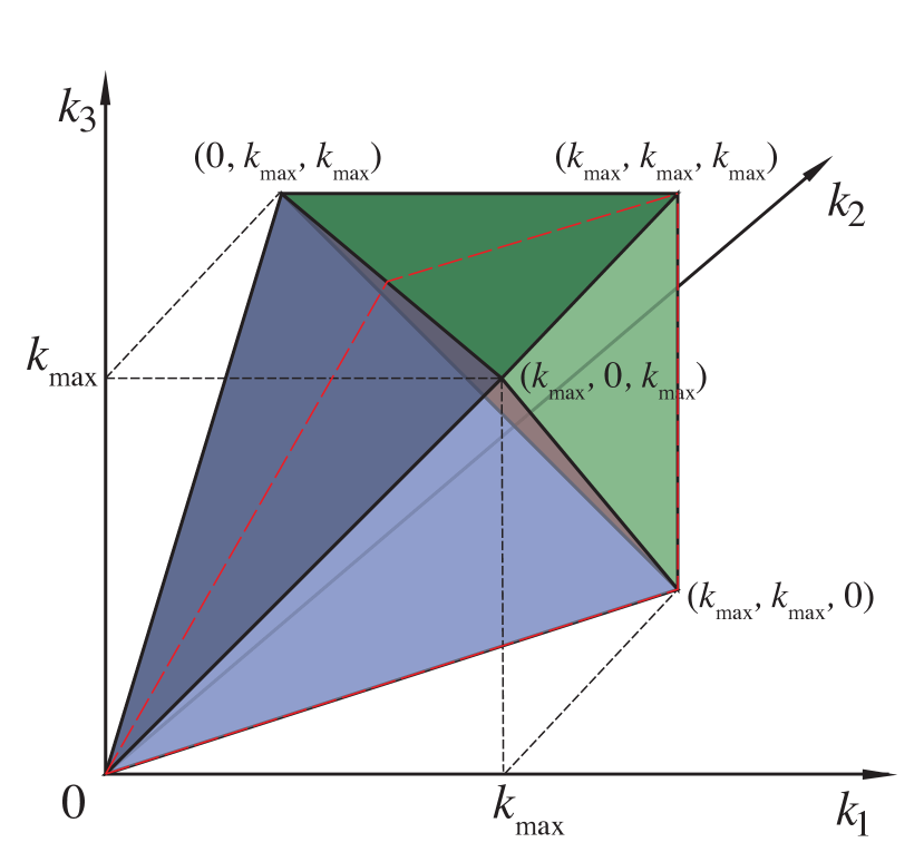
(a) The full tetrapyd bispectrum domain consists of a tetrahedral region (blue) defined by the wavevector triangle condition $\mathbf{k}_{1}+\mathbf{k}_{2}+\mathbf{k}_{3}=0$, together with a pyramidal region (green) bounded by the resolution limit $k_{\text{max}}$. To show the internal structure of the tetrapyd we split it along the red dashed line to obtain Figure II.1(b). (Lazanu et al., 2016)

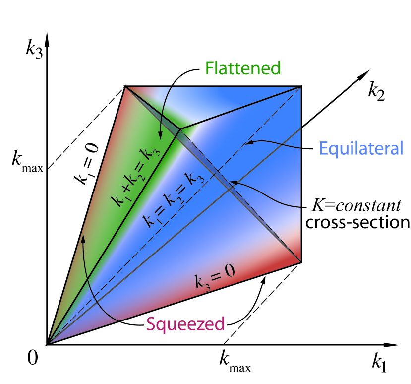
(b) The split 3D tetrapyd region showing only the back half with $k_{1}<k_{2}$. Colour-coded regions show the location of the ‘squeezed’ (red), ‘flattened’ (green) and ‘equilateral’ or ‘constant’ (blue) shape signals. The scale dependence of the bispectrum is reflected by the $K\equiv k_{1}+k_{2}+k_{3}=\text{const.}$ cross sectional planes. (Lazanu et al., 2016)

Figure II.1: Tetrahedral geometry of the allowed bispectrum combination $B(k_{1},k_{2},k_{3})$.

(a) Tree-level shape, $k_{max}=0.4$

(b) Nine-parameter model, $k_{max}=0.4$

(c) Scaled Tree-level shape, $k_{max}=2$

(d) Scaled squeezed shape, $k_{max}=2$

(e) Scaled constant shape, $k_{max}=2$

(f) 3-shape model, $k_{max}=2$

Figure II.2: The bispectrum shapes introduced in Section II.2 plotted at redshift $z=0.5$ up to various $k_{max}$.

II.3.1 Correlators Between Bispectra

Using Equation II.30 we can further define 4 correlators between bispectra. The shape correlator, $\mathcal{S}$, is defined by

$$\mathcal{S}(B_{i},B_{j})\equiv\frac{\left[B_{i},B_{j}\right]}{\sqrt{\left[B_{i},B_{i}\right]\left[B_{j},B_{j}\right]}},$$ (II.34)

and is restricted to $-1\leq\mathcal{S}\leq 1$. It can be thought of as the cosine between $B_{i}$ and $B_{j}$. To quantify how well the magnitudes of $B_{i}$ and $B_{j}$ match each other we define the amplitude correlator $\mathcal{A}$ as

$$\mathcal{A}(B_{i},B_{j})\equiv\sqrt{\frac{\big{[}B_{i},B_{i}\big{]}}{\big{[}B_{j},B_{j}\big{]}}}.$$ (II.35)

We can combine the information given by the shape and amplitude correlators into a single quantity known as the total correlator $\mathcal{T}$:

$$\mathcal{T}(B_{i},B_{j})\equiv 1-\sqrt{\frac{\left[B_{j}-B_{i},B_{j}-B_{i}\right]}{\left[B_{j},B_{j}\right]}}$$

$$\quad=1-\sqrt{1-2\mathcal{S}(B_{i},B_{j})\mathcal{A}(B_{i},B_{j})+\mathcal{A}^{2}(B_{i},B_{j})}.$$ (II.36)

The total correlator is a stringent test of correlation between bispectra, as both misalignment ($\mathcal{S}<1$) or a difference in amplitude ($\mathcal{A}\neq 1$) lead to a decrease in $\mathcal{T}$. Later on we will use $\mathcal{T}$ to test the ability of MODAL-LSS to reconstruct theoretical bispectra (see Section II.4).

We can interpret $\mathcal{T}$ physically as follows. Let $B_{T}$ be the true bispectrum and $B_{A}$ be an approximation to $B_{T}$. Now suppose we constrain each of these templates with Equation II.29 to obtain $f^{T}_{NL}$ and $f^{A}_{NL}$. The variance of each estimate is given by

$$\sigma^{2}_{i}=\expectationvalue{{f^{i}_{NL}}^{2}}=N_{i}^{-1}=\left[B_{i},B_{i}\right]^{-1}$$ (II.37)

and the variance of the difference between the two estimates is given by

$$\sigma^{2}_{diff} =\expectationvalue{\left(f^{T}_{NL}-f^{A}_{NL}\right)^{2}}$$

$$=\frac{1}{(N_{T}N_{A})^{2}}\left[N_{A}B_{T}-N_{T}B_{A},N_{A}B_{T}-N_{T}B_{A}\right]$$

$$=\frac{N_{A}-2\left[B_{A},B_{T}\right]+N_{T}}{N_{A}N_{T}}$$ (II.38)

If we take the ratio of $\sigma_{diff}$ and $\sigma_{A}$ then we get

$$\frac{\sigma^{2}_{diff}}{\sigma^{2}_{A}} =1-2\frac{1}{N_{T}}\left[B_{A},B_{T}\right]+\frac{N_{A}}{N_{T}}$$

$$\left(1-\mathcal{T}(B_{T},B_{A})\right)^{2}$$ (II.39)

This allows us to identify $1-\mathcal{T}$ as the coefficient of variation $c_{v}$ (Everitt and Skrondal, 2010). Therefore if $B_{A}$ is used as a proxy for $B_{T}$, $1-\mathcal{T}$ gives us the standard deviation between our estimate of $f_{NL}$ and the true value as a fraction of our error bar, ie:

$$\sigma_{diff}=\left(1-\mathcal{T}\right)\sigma$$ (II.40)

$\mathcal{T}$ is appropriate for comparing theoretical bispectra, but its performance is easily degraded by cosmic variance and hence another correlator is needed when simulation/observational data is involved. The $f_{nl}$ correlator, named as such due to its similarity to the $\langle\hat{f}_{nl}\rangle$ parameter in Equation II.30 above, again combines the shape and amplitude correlators:

$$f_{nl}(B_{i},B_{j}) \equiv\frac{\big{[}B_{i},B_{j}\big{]}}{\big{[}B_{j},B_{j}\big{]}}$$

$$=\mathcal{S}(B_{i},B_{j})\mathcal{A}(B_{i},B_{j}).$$ (II.41)

This can be interpreted as simply correlation between our estimate of $f_{NL}$ with the true value, normalised by the true value.

$$\frac{\expectationvalue{f^{T}_{NL}f^{A}_{NL}}}{\expectationvalue{{f^{T}_{NL}}^{2}}} =\frac{1}{N_{A}}\left[B_{T},B_{A}\right]$$

$$=f_{nl}(B_{T},B_{A})$$ (II.42)

II.4 MODAL-LSS Methodology

For general bispectra the 9-dimensional integral in the $\hat{f}_{NL}$ estimator (Equation II.29) is computationally intractable. This computation barrier has been solved by a separable method introduced in (Fergusson et al., 2010). This MODALl method has been applied to Planck CMB analysis with great success (Planck Collaboration, 2016b). This approach was adapted analyse the bispectrum of the large scale structure of the universe in (Schmittfull et al., 2013a), which iwas aptly named MODAL-LSS. Here we outline the MODAL-LSS methodology.

II.4.1 MODAL-LSS Basis

We first approximate the SN-weighted theoretical bispectrum in Equation II.33 by expanding it in a general seperable basis (see also Figure II.3):

$$\sqrt{\frac{k_{1}k_{2}k_{3}}{P(k_{1})P(k_{2})P(k_{3})}}B^{th}(k_{1},k_{2},k_{3})$$

$$\quad\approx\sum_{n}^{n_{max}}\alpha^{Q}_{n}Q^{\texttt{MODAL-LSS}{}}_{n}(k_{1}/k_{max},k_{2}/k_{max},k_{3}/k_{max}).$$ (II.43)

The basis functions ${Q^{\texttt{MODAL-LSS}{}}_{n}}$ are symmetrised products over one dimensional functions $q_{r}$:

$$Q^{\texttt{MODAL-LSS}{}}_{n}(x,y,z)\equiv q_{\{r}(x)q_{s}(y)q_{t\}}(z),$$ (II.44)

with $\{\dots\}$ representing symmetrisation over the indices $r,s,t$, and each $n$ corresponds to a combination of $r,s,t$. $k_{max}$ is the resolution of the tetrahedral domain defined above. The choice of $q_{r}$ is arbitrary and there are many sensible choices including $k$-bins (which are localised in $k$-space), wavelets (which are localised in real space), Fourier modes, etc. We adopt polynomials since they offer efficient compression of the data so fewer modes can be used without information loss. Note that the ${Q^{\texttt{MODAL-LSS}{}}_{n}}$ form a complete basis for the expansion of $B^{th}$, but naturally we truncate the expansion at some $n_{max}$ depending on the accuracy required. For convenience in our discussion below we will assume that the truncation causes errors are tiny and assume that Equation II.43 is exact.

$$\vbox{\hbox{\includegraphics[width=86.72267pt]{{theo_bis_1000_2048_49_z0p000_0.25_cropped}.jpeg}}}=\,\alpha_{1}\vbox{\hbox{\includegraphics[width=86.72267pt]{{theo_bis_1000_2048_Q0_z0p000_0.25_cropped}.jpeg}}}+\,\alpha_{2}\vbox{\hbox{\includegraphics[width=86.72267pt]{{theo_bis_1000_2048_Q2_z0p000_0.25_cropped}.jpeg}}}+\,\alpha_{3}\vbox{\hbox{\includegraphics[width=86.72267pt]{{theo_bis_1000_2048_Q6_z0p000_0.25_cropped}.jpeg}}}+\cdots$$ (II.45)

Figure II.3: A cartoon demonstrating the MODAL-LSS expansion. Here we are expanding the tree level bispectrum (Equation II.3) as a linear combination of the $Q^{\texttt{MODAL-LSS}{}}_{n}$ basis functions (represented by the tetrapyds), each of which is weighted by an $\alpha_{n}$ coefficient.

It has been shown that the convergence of the sum in Equation II.43 is independent of the choice of polynomials $q_{r}$. Different choices of polynomials only change the individual $\alpha^{Q}_{n}$ but not the sum. As such we choose our polynomials in order to ensure numerical stability of the method on the tetrahedral domain $\mathcal{V}_{B}$. Currently we find shifted Legendre polynomials $\tilde{P}_{l}(x)=P_{l}(2x-1)$ perform well and are adopted for $q_{r}$ as they demonstrate better orthogonality at low $n$ and encapsulate the behaviour of the bispectrum at non-linear scales very well. Calculation of higher order polynomials also demonstrates good numerical stability when calculated recursively.

Another issue is the mapping between $n$ and $r,s,t$. The ordering of this mapping is arbitrary, here we have adopted ‘slice ordering’ which orders the triples by the sum $r+s+t$. A sub-ordering is introduced along each column in cases of degeneracy, i.e.

$$\underline{0\rightarrow 000}\quad 4\rightarrow 111\quad~{}\,8\rightarrow 022\quad 12\rightarrow 113$$

$$\underline{1\rightarrow 001}\quad 5\rightarrow 012\quad~{}\,9\rightarrow 013\quad 13\rightarrow 023$$

$$2\rightarrow 011\quad\underline{6\rightarrow 003}\quad\underline{10\rightarrow 004}\quad 14\rightarrow 014$$ (II.46)

$$\underline{3\rightarrow 002}\quad 7\rightarrow 112\quad 11\rightarrow 122\quad\underline{15\rightarrow 005}~{}\cdots\,,$$

where the lines mark the end of each overall polynomial order.

Using the MODAL-LSS expansion in Equation II.43 we can rewrite $\hat{f}_{nl}$ in Equation II.29 as:

$$\hat{f}_{nl} =\frac{(2\pi)^{6}}{N_{th}}\int_{\mathbf{k}_{1},\mathbf{k}_{2},\mathbf{k}_{3}}\delta_{D}(\mathbf{k}_{1}+\mathbf{k}_{2}+\mathbf{k}_{3})$$

$$\qquad\qquad\times\frac{\sum_{n}\alpha^{Q}_{n}q_{\{r}(\frac{k_{1}}{k_{max}})q_{s}(\frac{k_{2}}{k_{max}})q_{t\}}(\frac{k_{3}}{k_{max}})}{\sqrt{k_{1}P(k_{1})k_{2}P(k_{2})k_{3}P(k_{3})}}$$

$$\qquad\qquad\times\left(\delta_{\mathbf{k}_{1}}\delta_{\mathbf{k}_{2}}\delta_{\mathbf{k}_{3}}-\langle\delta_{\mathbf{k}_{1}}\delta_{\mathbf{k}_{2}}\rangle\delta_{\mathbf{k}_{3}}\right)$$

$$=\frac{(2\pi)^{3}}{N_{th}}\sum_{n}\alpha^{Q}_{n}\int d^{3}x\int\frac{\prod_{i}d^{3}k_{i}}{(2\pi)^{9}}e^{i(\mathbf{k}_{1}+\mathbf{k}_{2}+\mathbf{k}_{3})\cdot\mathbf{x}}$$

$$\qquad\qquad\times\frac{q_{\{r}(\frac{k_{1}}{k_{max}})q_{s}(\frac{k_{2}}{k_{max}})q_{t\}}(\frac{k_{3}}{k_{max}})}{\sqrt{k_{1}P(k_{1})k_{2}P(k_{2})k_{3}P(k_{3})}}$$

$$\qquad\qquad\times\left(\delta_{\mathbf{k}_{1}}\delta_{\mathbf{k}_{2}}\delta_{\mathbf{k}_{3}}-\langle\delta_{\mathbf{k}_{1}}\delta_{\mathbf{k}_{2}}\rangle\delta_{\mathbf{k}_{3}}\right)$$

$$=\frac{(2\pi)^{3}}{N_{th}}\sum_{n}\alpha^{Q}_{n}\int d^{3}x\bigg{[}M_{r}(\mathbf{x})M_{s}(\mathbf{x})M_{t}(\mathbf{x})$$

$$\qquad\qquad-\langle M_{\{r}(\mathbf{x})M_{s}(\mathbf{x})\rangle M_{t\}}(\mathbf{x})\bigg{]},$$ (II.47)

where in the second line we have used the integral from of the delta function with variable $\mathbf{x}$, and we defined

$$M_{r}(\mathbf{x})\equiv\int\frac{d^{3}k}{(2\pi)^{3}}\frac{\delta_{\mathbf{k}}q_{r}(k/k_{max})}{\sqrt{kP(k)}}e^{i\mathbf{k}\cdot\mathbf{x}},$$ (II.48)

which is an inverse Fourier transform. Note that there is no symmetrisation over $r,s,t$ in the first term inside the square brackets as the product is already symmetric. As we are only analysing simulation data which approximately homogeneous and isotropic we can ignore the second term in the square brackets as it evaluates to zero. We then introduce

$$\beta^{Q}_{n}=(2\pi)^{3}\int d^{3}x\,M_{r}(\mathbf{x})M_{s}(\mathbf{x})M_{t}(\mathbf{x})$$ (II.49)

which allows us to express $\hat{f}_{nl}$ in a simple and elegant form:

$$\hat{f}_{nl}=\frac{1}{N_{th}}\sum_{n}\alpha^{Q}_{n}\beta^{Q}_{n}.$$ (II.50)

The beta coefficients $\beta^{Q}_{n}$ are approximately analogous (there is a subtly we will meet in the next section) to the alpha coefficients $\alpha^{Q}_{n}$ but they are used in the expansion of observational/simulation bispectra instead of theoretical ones.

In summary, we have reduced the complicated integral in Equation II.29 to a the calculation of $\alpha^{Q}_{n}$ and $\beta^{Q}_{n}$ coefficients. The computation of $\alpha^{Q}_{n}$ coefficients is a non-trivial problem but has been made efficient by the authors of (Briggs et al., 2016) whose implementation which we use here. The $\beta^{Q}_{n}$ coefficients on the other hand only require a number of (inverse) Fourier transforms (evident upon inspection of Equation II.48) which can be evaluated efficiently with the fast Fourier transform (FFT) algorithm, together with an integral over the spatial extent of the data set (Equation II.49) which can highly parallelised with Open Multi-Processing (OpenMP).

II.4.2 An orthogonal basis

Unlike the theoretical bispectrum the observational/simulation bispectrum is a statistical quantity, and and it can only be estimated through different realisations of the density field $\delta$. We expand the estimated observational bispectrum $\hat{B}_{\delta}$ in the following way:

$$\sqrt{\frac{k_{1}k_{2}k_{3}}{P(k_{1})P(k_{2})P(k_{3})}}\hat{B}_{\delta}(k_{1},k_{2},k_{3})$$

$$\quad=\sum_{n}^{n_{max}}\tilde{\beta}^{Q}_{n}Q_{n}(k_{1}/k_{max},k_{2}/k_{max},k_{3}/k_{max}),$$ (II.51)

the expectation value of which is the true underlying observational bispectrum $B_{\delta}\equiv\langle\hat{B}_{\delta}\rangle$:

$$\sqrt{\frac{k_{1}k_{2}k_{3}}{P(k_{1})P(k_{2})P(k_{3})}}B_{\delta}(k_{1},k_{2},k_{3})$$

$$\quad=\sum_{n}^{n_{max}}\langle\tilde{\beta}^{Q}_{n}\rangle Q_{n}(k_{1}/k_{max},k_{2}/k_{max},k_{3}/k_{max}).$$ (II.52)

We have introduced these new beta coefficients $\tilde{\beta}^{Q}_{n}$. To relate $\tilde{\beta}^{Q}_{n}$ to $\beta^{Q}_{n}$ we substitute Equation II.52 into Equation II.30:

$$\langle\hat{f}_{nl}\rangle =\frac{1}{N_{th}}\frac{V}{\pi}\int_{\mathcal{V}_{B}}dV_{k}\,\sum_{nm}\alpha_{n}^{Q}\langle\tilde{\beta}^{Q}_{n}\rangle Q_{n}Q_{m}$$

$$=\frac{1}{N_{th}}\sum_{nm}\alpha_{n}^{Q}\langle\tilde{\beta}^{Q}_{n}\rangle\gamma_{nm},$$ (II.53)

where

$$\gamma_{nm}\equiv\frac{V}{\pi}\int_{\mathcal{V}_{B}}dV_{k}Q_{n}Q_{m}$$ (II.54)

is the inner product between the $Q_{n}$ functions on the tetrapyd domain. Generally speaking $\gamma_{nm}$ is not diagonal since the $Q_{n}$ functions are not orthogonal to each other. Comparing this with the expectation value of Equation II.50 we obtain

$$\langle\beta^{Q}_{n}\rangle=\sum_{m}\gamma_{nm}\langle\tilde{\beta}^{Q}_{m}\rangle\Rightarrow\beta^{Q}_{n}=\sum_{m}\gamma_{nm}\tilde{\beta}^{Q}_{m}.$$ (II.55)

While $\beta^{Q}_{n}$ may be straightforward to evaluate numerically through Equation II.49, it often proves simpler to use an orthonormalised version we create by diagonalising $\gamma_{nm}$. We therefore introduce a basis $\{R_{n}\}$ which is defined relative to $\{Q_{n}\}$ by

$$R_{n}\equiv\lambda_{nm}Q_{m}\Leftrightarrow Q_{p}\equiv(\lambda^{-1})_{pq}R_{q}$$ (II.56)

such that it is orthonormal on the tetrapyd domain:

$$\frac{V}{\pi}\int_{\mathcal{V}_{B}}dV_{k}R_{n}R_{m}=\delta_{nm}.$$ (II.57)

From Equations II.54 and II.57 we deduce that $\gamma=\lambda^{-1}(\lambda^{-1})^{T}$. Choosing $R_{n}$ to have the same polynomial order as $Q_{n}$ forces this $\lambda$ to be the Cholesky decomposition. This is equivalent to a performing a modified Gram-Schmitt orthonormalisation of the $Q_{n}$ directly. We now apply the expansion in the $\{R_{n}\}$ basis:

$$\sqrt{\frac{k_{1}k_{2}k_{3}}{P(k_{1})P(k_{2})P(k_{3})}}B^{th}(k_{1},k_{2},k_{3})$$

$$\quad=\sum_{n}^{n_{max}}\alpha^{R}_{n}R_{n}(k_{1}/k_{max},k_{2}/k_{max},k_{3}/k_{max}),$$ (II.58)

$$\sqrt{\frac{k_{1}k_{2}k_{3}}{P(k_{1})P(k_{2})P(k_{3})}}B_{\delta}(k_{1},k_{2},k_{3})$$

$$\quad=\sum_{n}^{n_{max}}\langle\beta^{R}_{n}\rangle R_{n}(k_{1}/k_{max},k_{2}/k_{max},k_{3}/k_{max}).$$ (II.59)

Note that due to the orthonormality of the $R_{n}$ functions we do not need two sets of $\beta$ coefficients in this basis. Since $\sum_{n}\alpha^{Q}_{n}Q_{n}=\sum_{n}\alpha^{R}_{n}R_{n}$, one can derive the following relationships between the coefficients in the $\{Q_{n}\}$ and $\{R_{n}\}$ bases:

$$\alpha^{R}_{n}=\sum_{m}(\lambda^{-1})^{T}_{nm}\alpha^{Q}_{m},\quad\beta^{R}_{n}=\sum_{m}(\lambda^{-1})^{T}_{nm}\tilde{\beta}^{Q}_{m},$$ (II.60)

which allows us to write

$$\langle\hat{f}_{nl}\rangle=\frac{1}{N_{th}}\sum_{n}\alpha^{R}_{n}\langle\beta^{R}_{n}\rangle.$$ (II.61)

One can very easily show this is consistent with Equation II.53 above. Using the MODAL-LSS ansatz with Equation II.31 above we find that $N_{th}=\sum_{n}\alpha^{R}_{n}\alpha^{R}_{n}$. Therefore if the theoretical and data bispectrum match perfectly, i.e. $B^{th}=B_{\delta}$ and hence $\langle\hat{f}_{nl}\rangle=1$, we deduce that $\langle\beta^{R}_{n}\rangle=\alpha^{R}_{n}$.

II.4.3 Numerical implementation

An implementation of the MODAL-LSS method has already produced some good results (Schmittfull et al., 2013a). The code has since been completely overhauled and parallelised with OpenMP and multi-threaded FFTW for a dramatic reduction in run time, allowing us to estimate the bispectra of much larger simulations and also using more modes. We are now able to estimate the bispectrum of $2048^{3}$ density grids with $n_{max}=\mathcal{O}(1000)$ modes in $\sim 35$ minutes using 512 CPU-cores, a significant improvement in run time and resolution over the analysis of $512^{3}$ grids with $n_{max}=\mathcal{O}(50)$ in (Schmittfull et al., 2013a). We would like to emphasise that the computational costs for bispectrum estimation with MODAL-LSS scales with the size of the density grid and is a tiny fraction of the costs of N-body runs, and thus can be included in existing pipelines with little additional cost.

Another innovation to improve the performance of MODAL-LSS is the introduction of custom modes based on the separable bispectrum shapes given in Section II.2. Explicitly we split the SN-weighted versions of tree-level bispectrum (Equation II.3) and late-time local bispectrum (Section II.2.3) as follows (Note that $P(k)$ represents the non-linear power spectrum of choice):

• The tree-level bispectrum requires 6 custom polynomials:

  • $q^{\text{tree}}_{0}(k)=\sqrt{\frac{k}{P(k)}}\frac{5}{14}$

  • $q^{\text{tree}}_{1}(k)=\sqrt{\frac{k}{P(k)}}P(k)$

  • $q^{\text{tree}}_{2}(k)=-\sqrt{\frac{k}{P(k)}}P(k)k^{2}$

  • $q^{\text{tree}}_{3}(k)=\sqrt{\frac{k}{P(k)}}\frac{P(k)}{k^{2}}$

  • $q^{\text{tree}}_{4}(k)=\sqrt{\frac{k}{P(k)}}\frac{3}{14}k^{2}$

  • $q^{\text{tree}}_{5}(k)=\sqrt{\frac{k}{P(k)}}\frac{1}{14}k^{4}$

  which are combined into these 4 modes:

  • $Q^{\text{tree}}_{0}=q_{\{1}(x)q_{1}(y)q_{0\}}(z)$

  • $Q^{\text{tree}}_{1}=q_{\{2}(x)q_{3}(y)q_{0\}}(z)$

  • $Q^{\text{tree}}_{2}=q_{\{1}(x)q_{3}(y)q_{4\}}(z)$

  • $Q^{\text{tree}}_{3}=q_{\{3}(x)q_{3}(y)q_{5\}}(z)$

• The late-time local bispectrum requires 2 custom polynomials:

  • $q^{\text{local,late}}_{0}(k)=\sqrt{\frac{k}{P(k)}}\sqrt{P_{\text{lin}}(k)}k^{n_{s}/2-2}$

  • $q^{\text{local,late}}_{1}(k)=\sqrt{\frac{k}{P(k)}}\sqrt{P_{\text{lin}}(k)}k^{2-n_{s}/2}$

  resulting in a single mode:

  • $Q^{\text{local,late}}_{0}=q_{\{0}(x)q_{0}(y)q_{1\}}(z)$

These custom modes help pick up general features in the matter bispectra, which combined with the $Q_{n}$ functions ensures an effective reconstruction of any dark matter bispectrum signal.

Figure II.4: The nine-parameter up to $k_{max}=0.4\,h\,\text{Mpc}^{-1}$ by direct calculation (left), its reconstruction by MODAL-LSS with 1000 modes (middle) and the residuals between them (right). Note the change of scale in the colour bars.

Figure II.5: The 3-shape model up to $k_{max}=2.0\,h\,\text{Mpc}^{-1}$ by direct calculation (left), its reconstruction by MODAL-LSS with 1000 modes (middle) and the residuals between them (right). Note the change of scale in the colour bars.

Bispectrum shape	$n_{max}$	$k_{max}=0.4\,h\,\text{Mpc}^{-1}$		$k_{max}=2.0\,h\,\text{Mpc}^{-1}$		Computational cost
		$1-\mathcal{S}_{\alpha,th}$	$1-\mathcal{T}_{\alpha,th}$	$1-\mathcal{S}_{\alpha,th}$	$1-\mathcal{T}_{\alpha,th}$	(CPU-minutes)
Tree-level bispectrum	$50^{*}$	$6.7\text{\times}{10}^{-4}$	$3.6\text{\times}{10}^{-2}$	$1.3\text{\times}{10}^{-3}$	$5.1\text{\times}{10}^{-2}$	160
	10	0	0	0	0	90
	50	0	0	0	0	160
	200	0	0	0	0	370
	1000	0	0	0	0	1600
Nine-parameter model	$50^{*}$	$6.6\text{\times}{10}^{-4}$	$3.6\text{\times}{10}^{-2}$	-	-	450
	10	$3.3\text{\times}{10}^{-4}$	$2.6\text{\times}{10}^{-2}$	-	-	390
	50	$2.2\text{\times}{10}^{-4}$	$2.1\text{\times}{10}^{-2}$	-	-	450
	200	$7.9\text{\times}{10}^{-5}$	$1.3\text{\times}{10}^{-2}$	-	-	660
	1000	$2.2\text{\times}{10}^{-5}$	$6.7\text{\times}{10}^{-3}$	-	-	1870
3-shape model	$50^{*}$	$3.5\text{\times}{10}^{-4}$	$2.6\text{\times}{10}^{-2}$	$5.6\text{\times}{10}^{-5}$	$1.1\text{\times}{10}^{-2}$	190
	10	$5.8\text{\times}{10}^{-4}$	$3.4\text{\times}{10}^{-2}$	$3.8\text{\times}{10}^{-4}$	$2.8\text{\times}{10}^{-2}$	120
	50	$1.1\text{\times}{10}^{-4}$	$1.5\text{\times}{10}^{-2}$	$6.0\text{\times}{10}^{-5}$	$1.1\text{\times}{10}^{-2}$	190
	200	$1.6\text{\times}{10}^{-5}$	$5.7\text{\times}{10}^{-3}$	$1.2\text{\times}{10}^{-5}$	$4.9\text{\times}{10}^{-3}$	400
	1000	0	0	0	0	1610

Table II.1: The performance of MODAL-LSS at reconstructing different theoretical bispectrum shapes at different $k_{max}$ while varying the number of modes used in the reconstruction. $50^{*}$ indicates only shifted Legendre polynomials and no custom modes were used, highlighting the strength of the custom modes in capturing desired bispectrum signals. We use the shape $\mathcal{S}_{\alpha,th}$ and total correlator $\mathcal{T}_{\alpha,th}$ introduced in Equation II.63 to assess the accuracy of the reconstructed bispectra. It is clear that the total correlator is a much more stringent test than the shape correlator. With 1000 modes we obtain $\mathcal{T}_{\alpha,th}>0.99$ in all cases, giving us high confidence in the validity of the MODAL-LSS expansion. Note that we omit the nine-parameter model at $k_{max}=2.0\,h\,\text{Mpc}^{-1}$ since it is ill-defined at such non-linear scales. We give the computational cost of the method by the CPU-minutes required to reconstruct the theoretical bispectra on a $2048^{3}$ grid in pure OpenMP mode. It demonstrates better than linear scaling with $n_{max}$ which shows the highly optimised nature of the code. The performance also scales with $N_{grid}^{3}$, where $N_{grid}$ is the number of grid points, and will therefore run much faster for analyses that do not require such high resolution.

We conclude this section by assessing the accuracy of the MODAL-LSS expansion. This is only possible with theoretical bispectra where we know the true answer since statistical noise will always be present in simulations. A qualitative comparison is illustrated in Figures II.4 and II.5 where we plot the theoretical and reconstructed bispectra as well as the residuals between them different $k_{max}$. Quantitatively we evaluate both the shape and total correlator between a theoretical bispectrum $B^{th}$ and its MODAL-LSS counterpart $\sum_{n}\alpha^{R}_{n}B^{R}_{n}$, where

$$B^{R}_{n}(k_{1},k_{2},k_{3})=$$

$$\quad\sqrt{\frac{P(k_{1})P(k_{2})P(k_{3})}{k_{1}k_{2}k_{3}}}R_{n}(k_{1}/k_{max},k_{2}/k_{max},k_{3}/k_{max}).$$ (II.62)

Using Equations II.34 and II.36 we find that

$$\mathcal{S}_{\alpha,th} \equiv\mathcal{S}(\sum_{n}\alpha^{R}_{n}B^{R}_{n},B^{th})=\sqrt{\frac{\sum_{n}(\alpha^{R}_{n})^{2}}{\left[B^{th},B^{th}\right]}},$$

$$\mathcal{T}_{\alpha,th} \equiv\mathcal{T}(\sum_{n}\alpha^{R}_{n}B^{R}_{n},B^{th})=1-\sqrt{1-\frac{\sum_{n}(\alpha^{R}_{n})^{2}}{\left[B^{th},B^{th}\right]}},$$ (II.63)

where we have used the orthonormality of the ${R_{n}}$ basis functions to obtain $\left[\sum_{n}\alpha^{R}_{n}B^{R}_{n},B^{th}\right]=\sum_{n}(\alpha^{R}_{n})^{2}$.

We tested MODAL-LSS with a range of bispectrum shapes, including the tree-level bispectrum (Equation II.20), nine-parameter model (Equation II.6) and the 3-shape model (Equation II.19), at different $k_{max}$ and number of modes up to $n_{max}=1000$ (Table II.1). MODAL-LSS is able to reconstruct all bispectrum shapes with $\mathcal{T}_{\alpha,th}>99\%$ at different $k$-ranges, and improvements can certainly be made by using more modes. This result justifies our decision to take the approximation in Equation II.43 to be exact. This also gives us confidence that MODAL-LSS can very accurately estimate simulation and observational bispectra. The computational cost of MODAL-LSS is estimated by the CPU-minutes used when reconstructing the various bispectrum. The code for reconstructing theoretical bispectra is parallelised with hybrid MPI-OpenMP but the tests here were ran with pure OpenMP and 1 thread per CPU core. Note that this may not be the optimal number of threads and further reductions in run time may be possible.

II.5 Sources of error in bispectrum estimation

In order to make meaningful comparisons between simulation/observational data with theoretical predictions one must have a thorough understanding of the errors that occur in our measurements. Since the main focus of this paper is on simulations we will not discuss observational effects such as survey geometry and redshift-space distortions (RSD). The main contributions we consider here are Poisson shot noise, covariance of the MODAL-LSS estimator, and aliasing due to the use of FFTs, all of which are relevant for the analysis of observational data in the future.

II.5.1 Shot noise contribution to the power spectrum and bispectrum

Since dark matter halos and galaxies are discrete tracers of their respective density fields, measurements of their statistics are biased relative to the true values that are of interest to us. This is known as Poisson shot noise. This effect is well known for the power spectrum and bispectrum, and we quote here the relationships between the statistics of the discrete sample and the underlying continuous field:

$$P_{n}(k) =P(k)+\frac{1}{\bar{n}}$$ (II.64)

$$B_{n}(k_{1},k_{2},k_{3}) =B(k_{1},k_{2},k_{3})$$

$$\quad+\frac{1}{\bar{n}}[P(k_{1})+P(k_{2})+P(k_{3})]+\frac{1}{\bar{n}^{2}},$$ (II.65)

where the subscript $n$ denotes the discrete number density and $\bar{n}$ is the mean number density of the sample. When making comparisons between theoretical and simulation bispectra in Section III.3 one simply has to subtract the shot noise contribution in the simulation bispectra before calculating any correlators.

II.5.2 Covariance of estimators

The variance of an estimator is given by its covariance matrix $C_{X}$ which can be written schematically as:

$$C_{X} \equiv\text{cov}(\hat{X}(\theta),\hat{X}(\theta^{\prime}))$$

$$=\expectationvalue{\hat{X}(\theta)\hat{X}(\theta^{\prime})}-\expectationvalue{\hat{X}(\theta)}\expectationvalue{\hat{X}(\theta^{\prime})}.$$ (II.66)

In addition to calculating covariance matrices numerically through simulations we also need a framework to calculate them (semi-)analytically as a consistency check.

Power spectrum covariance

We first give a brief introduction to matter power spectrum estimation and the calculation of its covariance as this has been widely discussed in the literature. This will prepare us for the discussion on the bispectrum covariance later. Consider for example estimating the power spectrum by binning it in $k$-space and averaging over all modes within each bin Chan and Blot (2017); Feldman et al. (1994):

$$\hat{P}(k)=\frac{k_{F}^{3}}{(2\pi)^{3}}\int_{k}\frac{d^{3}p}{V_{s}(k)}\left|\delta(\mathbf{p})\right|^{2},$$ (II.67)

where $k_{F}=2\pi/L=(1/\delta^{D}(\mathbf{0}))^{1/3}$ is the fundamental frequency of the simulation box of length $L$, and the integral is performed over all modes that lie in the spherical shell $\left|\mathbf{p}-k\right|\leq\Delta k/2$ which has width $\Delta k$. The normalisation factor $V_{s}$ is the volume of the shell: $V_{s}=\int_{k}d^{3}p=4\pi k^{2}\Delta k+\pi(\Delta k)^{3}/3$. This estimator is unbiased because

$$\expectationvalue{\hat{P}(k)} =\frac{k_{F}^{3}}{(2\pi)^{3}}\int_{k}\frac{d^{3}p}{V_{s}(k)}\expectationvalue{\left|\delta(\mathbf{p})\right|^{2}}=\frac{k_{F}^{3}}{(2\pi)^{3}}\expectationvalue{\left|\delta(k)\right|^{2}}$$

$$=\frac{k_{F}^{3}}{(2\pi)^{3}}(2\pi)^{3}\delta(\mathbf{0})P(k)=P(k).$$ (II.68)

The covariance matrix for this estimator is

$$C_{P}(k,k^{\prime})$$

$$={} \frac{k_{F}^{6}}{(2\pi)^{6}}\int_{k}\frac{d^{3}p}{V_{s}(k)}\int_{k^{\prime}}\frac{d^{3}q}{V_{s}(k^{\prime})}\expectationvalue{\delta^{*}_{p}\delta_{p}\delta^{*}_{q}\delta_{q}}-P(k)P(k^{\prime})$$

$$={} \frac{2k_{F}^{3}}{V_{s}(k)}P^{2}(k)\delta_{k,k^{\prime}}$$

$$\qquad+\frac{k_{F}^{6}}{(2\pi)^{6}}\int_{k}\frac{d^{3}p}{V_{s}(k)}\int_{k^{\prime}}\frac{d^{3}q}{V_{s}(k^{\prime})}\expectationvalue{\delta^{*}_{p}\delta_{p}\delta^{*}_{q}\delta_{q}}_{c},$$

$$={} \frac{2k_{F}^{3}}{V_{s}(k)}P^{2}(k)\delta_{k,k^{\prime}}$$

$$\qquad+\frac{k_{F}^{3}}{(2\pi)^{3}}\int_{k}\frac{d^{3}p}{V_{s}(k)}\int_{k^{\prime}}\frac{d^{3}q}{V_{s}(k^{\prime})}T(\mathbf{p},-\mathbf{p},\mathbf{q},-\mathbf{q}),$$ (II.69)

where we have expanded the four-point correlator in terms of its connected pieces: $\expectationvalue{\delta^{*}_{p}\delta_{p}\delta^{*}_{q}\delta_{q}}=\expectationvalue{\delta^{*}_{p}\delta_{p}}\expectationvalue{\delta^{*}_{q}\delta_{q}}+\expectationvalue{\delta^{*}_{p}\delta^{*}_{q}}\expectationvalue{\delta_{p}\delta_{q}}+\expectationvalue{\delta^{*}_{p}\delta_{q}}\expectationvalue{\delta^{*}_{q}\delta_{p}}+\expectationvalue{\delta^{*}_{p}\delta_{p}\delta^{*}_{q}\delta_{q}}_{c}$, and the trispectrum $T$ is defined by $\expectationvalue{\delta(\mathbf{k}_{1})\delta(\mathbf{k}_{2})\delta(\mathbf{k}_{3})\delta(\mathbf{k}_{4})}_{c}=(2\pi)^{3}\delta_{D}(\mathbf{k}_{1}+\mathbf{k}_{2}+\mathbf{k}_{3}+\mathbf{k}_{4})T(\mathbf{k}_{1},\mathbf{k}_{2},\mathbf{k}_{3},\mathbf{k}_{4})$ where the subscript $c$ denotes connected. Connected $n$-point correlators with $n>2$ vanish if $\delta$ is a Gaussian field, but e.g. gravitational evolution induces mode coupling and hence non-Gaussianity in the form of higher order correlators.

The first term in Equation II.69 is the Gaussian contribution to the power spectrum covariance and can be estimated with $\hat{P}$; the Kronecker delta $\delta_{k,k^{\prime}}$ enforces the diagonality of the Gaussian covariance. The trispectrum term is the non-Gaussian covariance which is non-trivial to estimate directly from simulations or calculate theoretically. Crucially the non-Gaussian covariance does not scale inversely with the number of modes in each bin unlike the Gaussian covariance Chan and Blot (2017); Mohammed et al. (2017); this also applies to the bispectrum. However they both scale inversely with the simulation box size through $k_{F}^{3}$, and clearly can both be suppressed by averaging over different simulation realisations.

Covariance of the MODAL-LSS estimator

Now we turn our attention to the covariance of the MODAL-LSS bispectrum estimator (Equation II.51), which is unbiased because

$$\sqrt{\frac{k_{1}k_{2}k_{3}}{P(k_{1})P(k_{2})P(k_{3})}}\expectationvalue{\hat{B}_{\delta}(k_{1},k_{2},k_{3})}$$

$$={} \sum_{n}^{n_{max}}\expectationvalue{\tilde{\beta}^{Q}_{n}}Q_{n}(k_{1}/k_{max},k_{2}/k_{max},k_{3}/k_{max})$$

$$={} \sum_{n}^{n_{max}}\alpha^{Q}_{n}Q_{n}(k_{1}/k_{max},k_{2}/k_{max},k_{3}/k_{max}),$$

$$={} \sqrt{\frac{k_{1}k_{2}k_{3}}{P(k_{1})P(k_{2})P(k_{3})}}B_{\delta}(k_{1},k_{2},k_{3}).$$ (II.70)

The covariance of $\hat{B}_{\delta}$, $C_{B}$, is given by:

$$C_{B}(k_{1},k_{2},k_{3},k_{1}^{\prime},k_{2}^{\prime},k_{3}^{\prime})$$

$$={} \sqrt{\frac{P_{1}P_{2}P_{3}P_{1}^{\prime}P_{2}^{\prime}P_{3}^{\prime}}{k_{1}k_{2}k_{3}k_{1}^{\prime}k_{2}^{\prime}k_{3}^{\prime}}}\sum_{mn}^{n_{max}}\expectationvalue{\tilde{\beta}^{Q}_{m}\tilde{\beta}^{Q}_{n}}Q_{m}Q_{n}^{\prime}$$

$$\quad-B(k_{1},k_{2},k_{3})B(k_{1}^{\prime},k_{2}^{\prime},k_{3}^{\prime})$$

$$={} \sqrt{\frac{P_{1}P_{2}P_{3}P_{1}^{\prime}P_{2}^{\prime}P_{3}^{\prime}}{k_{1}k_{2}k_{3}k_{1}^{\prime}k_{2}^{\prime}k_{3}^{\prime}}}\sum_{mnop}^{n_{max}}(\gamma^{-1})_{om}(\gamma^{-1})_{pn}\expectationvalue{\beta^{Q}_{m}\beta^{Q}_{n}}Q_{o}Q_{p}^{\prime}$$

$$\quad-B(k_{1},k_{2},k_{3})B(k_{1}^{\prime},k_{2}^{\prime},k_{3}^{\prime}),$$ (II.71)

where $P_{1}=P(k_{1})$ etc., and the arguments of the $Q_{n}$ basis functions have been suppressed for brevity. We have also used Equation II.55 to convert from $\tilde{\beta}^{Q}_{n}$ to $\beta^{Q}_{n}$. In order to evaluate $\expectationvalue{\beta^{Q}_{m}\beta^{Q}_{n}}$ we write $\beta^{Q}_{n}$ as follows using Equation II.47:

$$\beta^{Q}_{n}$$

$$={} (2\pi)^{6}\int_{\mathbf{k}_{1},\mathbf{k}_{2},\mathbf{k}_{3}}\frac{\delta_{\mathbf{k}_{1}}\delta_{\mathbf{k}_{2}}\delta_{\mathbf{k}_{3}}Q_{n}}{\sqrt{k_{1}k_{2}k_{3}P_{1}P_{2}P_{3}}}\delta_{D}(\mathbf{k}_{1}+\mathbf{k}_{2}+\mathbf{k}_{3})$$

$$={} (2\pi)^{3}\int d^{3}x\int_{\mathbf{k}_{1},\mathbf{k}_{2},\mathbf{k}_{3}}\frac{\delta_{\mathbf{k}_{1}}\delta_{\mathbf{k}_{2}}\delta_{\mathbf{k}_{3}}Q_{n}}{\sqrt{k_{1}k_{2}k_{3}P_{1}P_{2}P_{3}}}e^{i(\mathbf{k}_{1}+\mathbf{k}_{2}+\mathbf{k}_{3})\cdot\mathbf{x}},$$ (II.72)

which leads to this rather messy expression:

$$\expectationvalue{\beta^{Q}_{m}\beta^{Q}_{n}}$$

$$={} (2\pi)^{12}\int_{1,2,3,1^{\prime},2^{\prime},3^{\prime}}\frac{Q^{\vphantom{\prime}}_{m}}{\sqrt{k^{\vphantom{\prime}}_{1}k_{2}k_{3}P_{1}P_{2}P_{3}}}\frac{Q_{n}^{\prime}}{\sqrt{k_{1}^{\prime}k_{2}^{\prime}k_{3}^{\prime}P_{1}^{\prime}P_{2}^{\prime}P_{3}^{\prime}}}$$

$$\quad\times\delta_{D}(\mathbf{k}_{1}+\mathbf{k}_{2}+\mathbf{k}_{3})\delta_{D}(\mathbf{k}_{1}^{\prime}+\mathbf{k}_{2}^{\prime}+\mathbf{k}_{3}^{\prime})$$

$$\quad\times\expectationvalue{\delta_{\mathbf{k}^{\vphantom{\prime}}_{1}}\delta_{\mathbf{k}^{\vphantom{\prime}}_{2}}\delta_{\mathbf{k}^{\vphantom{\prime}}_{3}}\delta_{\mathbf{k}_{1}^{\prime}}\delta_{\mathbf{k}_{2}^{\prime}}\delta_{\mathbf{k}_{3}^{\prime}}},$$ (II.73)

where we further abbreviate the integral over the 6 wavevectors to $\int_{1,2,3,1^{\prime},2^{\prime},3^{\prime}}\equiv\int\frac{\prod_{i=1}^{3}d^{3}k_{i}}{(2\pi)^{9}}\frac{\prod_{i=1}^{3}d^{3}k_{i}^{\prime}}{(2\pi)^{9}}$. With some difficulty this can be rewritten as:

$$\expectationvalue{\beta^{Q}_{m}\beta^{Q}_{n}}$$

$$={} 6(2\pi)^{3}\gamma_{mn}+\alpha^{Q}_{m}\alpha^{Q}_{n}+V(2\pi)^{12}\int_{1,2,3,1^{\prime},2^{\prime},3^{\prime}}\frac{Q^{\vphantom{\prime}}_{m}}{\sqrt{k^{\vphantom{\prime}}_{1}k_{2}k_{3}P_{1}P_{2}P_{3}}}\frac{Q_{n}^{\prime}}{\sqrt{k_{1}^{\prime}k_{2}^{\prime}k_{3}^{\prime}P_{1}^{\prime}P_{2}^{\prime}P_{3}^{\prime}}}\delta_{D}(\mathbf{k}_{1}+\mathbf{k}_{2}+\mathbf{k}_{3})\delta_{D}(\mathbf{k}_{1}^{\prime}+\mathbf{k}_{2}^{\prime}+\mathbf{k}_{3}^{\prime})$$

$$\quad\times\Bigg{(}(2\pi)^{3}\delta_{D}(\mathbf{k}_{3}-\mathbf{k}_{3}^{\prime})B(k_{1},k_{2},k_{3}^{\prime})B(k_{1}^{\prime},k_{2}^{\prime},k_{3})+8\,\text{perms}$$

$$\qquad+(2\pi)^{3}\delta_{D}(\mathbf{k}_{1}+\mathbf{k}_{1}^{\prime})T(\mathbf{k}_{2},\mathbf{k}_{3},\mathbf{k}_{2}^{\prime},\mathbf{k}_{3}^{\prime})P(k_{1})+8\,\text{perms}+P_{5}(\mathbf{k}_{1},\mathbf{k}_{2},\mathbf{k}_{3},\mathbf{k}_{1}^{\prime},\mathbf{k}_{2}^{\prime},\mathbf{k}_{3}^{\prime})\Bigg{)}.$$ (II.74)

where the pentaspectrum $P_{5}$ is defined by $\expectationvalue{\delta(\mathbf{k}_{1})\delta(\mathbf{k}_{2})\delta(\mathbf{k}_{3})\delta(\mathbf{k}_{4})\delta(\mathbf{k}_{5})\delta(\mathbf{k}_{6})}_{c}=(2\pi)^{3}\delta_{D}(\mathbf{k}_{1}+\mathbf{k}_{2}+\mathbf{k}_{3}+\mathbf{k}_{4}+\mathbf{k}_{5}+\mathbf{k}_{6})P_{5}(\mathbf{k}_{1},\mathbf{k}_{2},\mathbf{k}_{3},\mathbf{k}_{4},\mathbf{k}_{5},\mathbf{k}_{6})$. While there is no easy way to evaluate the last two set of terms involving the trispectrum and pentaspectrum, the Gaussian covariance of the $\beta^{R}_{n}$ is given trivially as

$$C^{\beta}_{mn}\equiv\expectationvalue{\beta^{R}_{m}\beta^{R}_{n}}-\expectationvalue{\beta^{R}_{m}}\expectationvalue{\beta^{R}_{n}}\approx 6(2\pi)^{3}\delta_{mn},$$ (II.75)

which is diagonal. Unfortunately $C_{B}$ cannot be evaluated analytically, even in the Gaussian limit, since Equation II.71 yields

$$\sqrt{\frac{k_{1}k_{2}k_{3}k_{1}^{\prime}k_{2}^{\prime}k_{3}^{\prime}}{P_{1}P_{2}P_{3}P_{1}^{\prime}P_{2}^{\prime}P_{3}^{\prime}}}C_{B}(k_{1},k_{2},k_{3},k_{1}^{\prime},k_{2}^{\prime},k_{3}^{\prime})$$

$$\approx{} 6(2\pi)^{3}\sum_{mn}^{n_{max}}Q_{m}^{\prime}(k_{1}^{\prime},k_{2}^{\prime},k_{3}^{\prime})(\gamma^{-1})_{mn}Q_{n}(k_{1},k_{2},k_{3})$$

$$={} 6(2\pi)^{3}\sum_{n}^{n_{max}}R_{n}^{\prime}(k_{1}^{\prime},k_{2}^{\prime},k_{3}^{\prime})R_{n}(k_{1},k_{2},k_{3})$$ (II.76)

where we have used Equation II.56 to convert from the $\{Q_{n}\}$ basis to $\{R_{n}\}$. The last line cannot be further simplified because in practice we can never use enough modes to ensure $\{R_{n}\}$ forms a complete basis. Nevertheless we can calculate the Gaussian covariance of $\hat{f}_{nl}=\sum_{n}\alpha^{R}_{n}\beta^{R}_{n}/\sum_{n}\alpha^{R}_{n}\alpha^{R}_{n}$ here which we will explore numerically in Section III.2:

$$C_{f_{nl}} \equiv\expectationvalue{\hat{f}_{nl}^{2}}-\expectationvalue{\hat{f}_{nl}}^{2}$$

$$=\frac{\sum_{mn}\alpha^{R}_{m}\alpha^{R}_{n}\expectationvalue{\beta^{R}_{m}\beta^{R}_{n}}-(\sum_{n}\alpha^{R}_{n}\expectationvalue{\beta^{R}_{n}})^{2}}{(\sum_{n}\alpha^{R}_{n}\alpha^{R}_{n})^{2}}$$

$$\approx\frac{1}{(\sum_{n}\alpha^{R}_{n}\alpha^{R}_{n})^{2}}\Bigg{(}\sum_{mn}\alpha^{R}_{m}\alpha^{R}_{n}\left(6(2\pi)^{3}\delta_{mn}+\alpha^{R}_{m}\alpha^{R}_{n}\right)$$

$$\qquad\qquad\qquad\qquad-(\sum_{n}\alpha^{R}_{n}\alpha^{R}_{n})^{2}\Bigg{)}$$

$$=\frac{6(2\pi)^{3}}{\sum_{n}\alpha^{R}_{n}\alpha^{R}_{n}}.$$ (II.77)

Suppression of large-scale variances

Large variances are prominent at large scales due to the finite volume of the simulation box or observational area leading to a lack of Fourier modes for statistical calculations. These are typically known as finite box or cosmic variance effects, although in the former case there is the added complication of mode coupling induced by non-linear gravitational evolution (Angulo and Pontzen, 2016). These errors need to be controlled as to extract cosmological parameters from galaxy surveys, and there is evidence to suggest detection of new physics may require $\mathcal{O}(0.1\%)$ accuracy in simulations (Baldauf et al., 2016). While cosmic variance, which is defined by the observational volume of a given survey, is unavoldable, we could reduce finite box errors in simulations by simply expanding the box or averaging multiple simulations. Unfortunatly both of these approaches are costly in terms of time and computational resources. For a more efficient way of obtaining ensemble averaged quantities such as the power spectrum and bispectrum the the authors of (Pontzen et al., 2016; Angulo and Pontzen, 2016) have proposed a method of pairing up simulations which have opposite phases in their initial conditions. The phase inversion has no affect on the statistical properties of the simulation thus the pairing up process does not bias power spectra and bispectra estimation. However, leading order contributions to the Gaussian covariances, which are the dominant contribution to cosmic variance, will cancel as they are out-of-phase with each other.

We will quickly review the method. First we expand the late-time non-linear density field in standard perturbation theory (SPT) (Bernardeau et al., 2002):

$$\delta(\mathbf{k},z)=\sum^{\infty}_{n=1}\delta_{n}(\mathbf{k},z),$$ (II.78)

where $\delta_{1}$ represents linear growth of the initial conditions, an $\delta_{n}$ are $n$ copies of $\delta_{1}$ convolved with the SPT kernels $F_{n}$. We can calculate the power spectrum in this formalism, expanding to 4th order in products of $\delta_{1}$ we obtain:

$$P=P_{11}+P_{12}+P_{21}+P_{13}+P_{22}+P_{31}+\cdots,$$ (II.79)

where $P=\left<\delta\delta\right>$ and $P_{nm}$ denotes $P=\left<\delta_{n}\delta_{m}\right>$. Assuming Gaussian initial conditions so that $\delta_{1}$ is also Gaussian, we can use Wick’s theorem to eliminate terms containing odd multiples of $\delta_{1}$, thus giving:

$$P^{\text{Gaussian IC}}=P_{11}+P_{13}+P_{22}+P_{31}+\cdots.$$ (II.80)

The effect of phase inversion is to reverse the sign of $\delta_{1}$, and the pairing up procedure serves to annihilate the same odd-parity terms that are expected to vanish in the ensemble average, while leaving the signal terms, which have even parity, intact. On the other hand since the non-Gaussian covariances also have even parity they remain unaffected.

The same applies for the bispectrum. The expansion in SPT is now (neglecting permutations)

$$B =B_{111}+B_{112}+B_{113}+B_{122}$$

$$\qquad+B_{114}+B_{123}+B_{222}+\cdots,$$ (II.81)

so that for Gaussian initial conditions we have

$$B^{\text{Gaussian IC}}=B_{112}+B_{122}+B_{114}+B_{123}+B_{222}+\cdots.$$ (II.82)

Again we see that terms containing an odd number of $\delta_{1}$ vanish which coincides with the effect of pairing up phase inverted simulations. While the suppression of variance in power spectra estimation was explored in great detail in (Angulo and Pontzen, 2016) no equivalent test have been performed with the bispectrum, which we leave to future work.

II.5.3 Systematic offsets due to aliasing contributions

$$\vbox{\hbox{\includegraphics[width=134.42113pt]{function_mult.jpeg}}}\,\times\vbox{\hbox{\includegraphics[width=134.42113pt]{Dirac_comb_mult.jpeg}}}\,=\vbox{\hbox{\includegraphics[width=134.42113pt]{result_mult.jpeg}}}$$

(a) Sampling in real space is a multiplication of the signal with a Dirac comb.

$$\vbox{\hbox{\includegraphics[width=134.42113pt]{function_conv.jpeg}}}\,*\vbox{\hbox{\includegraphics[width=134.42113pt]{Dirac_comb_conv.jpeg}}}\,=\vbox{\hbox{\includegraphics[width=134.42113pt]{result_conv.jpeg}}}$$

(b) In Fourier space this becomes a convolution between the signal and a Dirac comb, resulting in multiple, aliased copies of the signal.

Figure II.6: Sampling in real and Fourier space (Figure 1 from (Jasche et al., 2009)).

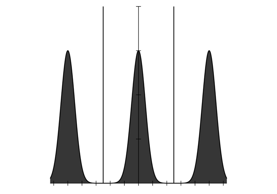
(a) If the sampling frequency is more than twice the highest frequency in the signal, then the aliased images that appear after convolving the signal with the Dirac comb do not overlap. In this case the signal is undistorted and can be uniquely restored.

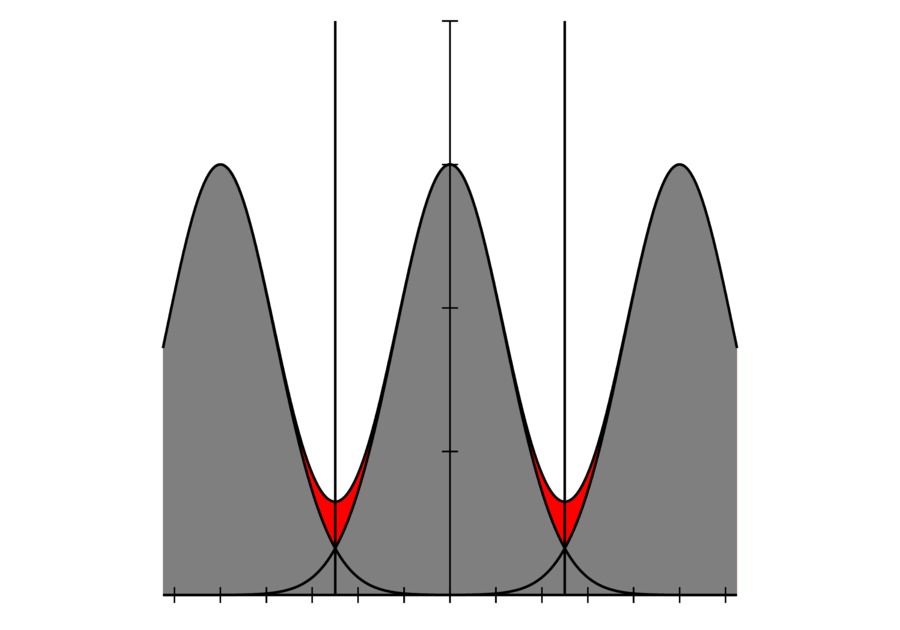
(b) On the other hand if the Nyquist criterion is not met, the images will then overlap with each other due to contributions from the higher frequencies, leading to significant distortions near the Nyquist frequency. There is no easy way to recover the original signal.

Figure II.7: If the sampling frequency is too low, aliasing occurs (Figure 2 from (Jasche et al., 2009)).

Virtually all power spectra and bispectra analyses are done with FFTs due to the efficiency of calculating Fourier transforms versus direct calculation of correlation functions in real space (Jing, 2005). The first step in using FFTs is to put the particles on a regular grid. This involves a mass assignment scheme which dictates the weighting with which each particle is distributed across its surrounding grid points. Many of these schemes are well known in the literature, e.g. Nearest Grid Point (NGP), Cloud in cell (CIC) and Triangular Shaped Clouds (TSC) (Jing, 2005), as well as higher order interpolation schemes such as Piecewise Cubic Spline (PCS) (Sefusatti et al., 2016) and Daubechies wavelet transformations (Cui et al., 2008). The effect of this assignment manifests as a convolution with the density field which becomes a product with the corresponding window function $W(\mathbf{k})$ in Fourier space. In principle this can be corrected for easily by dividing out the window function in Fourier space. However even in this case the use of discrete FFTs inevitably leads to information loss (Jasche et al., 2009). By the Shannon sampling theorem (Shannon, 1949) all the information in a signal can be recovered if the sampling frequency is twice that of the highest frequency in the signal, i.e. with a sufficiently high sampling frequency a band-limited signal can be reproduced without information loss. This is known as the Nyquist criterion. The sampling theorem states that this limit is the Nyquist frequency $k_{Ny}=k_{max}/2=\pi/H$, where $k_{max}$ is the sampling frequency of the grid and $H$ is the grid spacing. For the purpose of estimating correlation functions with FFTs it is known than the cutoff frequency for the power spectrum is the Nyquist frequency $k_{Ny}$ (Jing, 2005; Cui et al., 2008; Jasche et al., 2009; Sefusatti et al., 2016). For the bispectrum (Jeong, 2010) and (Sefusatti et al., 2016) propose the limit for the bispectrum should be $2k_{Ny}/3$.

There is a second serious problem associated with discrete grids which is the introduction of sampling artefacts near the Nyquist frequency. As explained in further detail in (Jasche et al., 2009), discrete sampling in real space is effectively a multiplication of the signal with a Dirac comb (Figure II.6(a)). In Fourier space this multiplication becomes a convolution operation, resulting in multiple images of the signal evenly spaced at the sampling frequency of the grid (Figure II.6(b)). In the case that the sampling frequency is more than twice the maximum frequency of the signal, as in Figure II.7(a), then the images of the signal do not overlap each other and no artefacts are induced. Otherwise if higher frequencies are indeed present (Figure II.7(b)), which certainly holds true in cosmological contexts, then the copies of the replicated signal will overlap and distort the sampled signal near the Nyquist frequency. We demonstrate this effect with GADGET-3 power spectra and bispectra in Figure II.8 (for details of the simulations see Section III.1.2 below). Here we find that the cutoff frequency for the bispectrum is the same as the power spectrum, $k_{Ny}$ in disagreement with the predictions of (Jing, 2005; Cui et al., 2008; Jasche et al., 2009; Sefusatti et al., 2016).

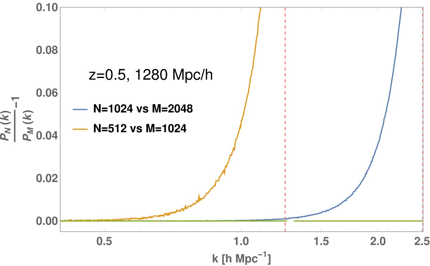
(a) Ratio between GADGET-3 power spectra estimated with FFT grids of different sizes. The baseline is the larger of the two CIC grids, and the pink, dashed lines indicate the Nyquist frequencies $k_{Ny}$ for the $512^{3}$ and $1024^{3}$ CIC grids. It is clear how aliasing contributions lead to overestimation of the power spectra near $k=k_{Ny}$, but the functional form of this overshoot cannot be calculated analytically.

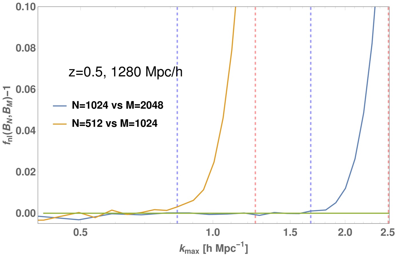
(b) $f_{nl}$ correlators between GADGET-3 bispectra estimated with the same FFT grids in Figure II.8(a). Again pink, dashed lines indicate $k_{Ny}$ for the various grids, but we additionally label $k=\frac{2}{3}k_{Ny}$ with blue, dashed lines to find the correct cutoff frequency. Contrary to (Jeong, 2010; Sefusatti et al., 2016) there is little to suggest that bispectrum estimation breaks down at $\frac{2}{3}k_{Ny}$, but rather at $k_{Ny}$ as for the power spectrum.

Figure II.8: A demonstration of aliasing in the power spectrum and bispectrum for GADGET-3 simulations.

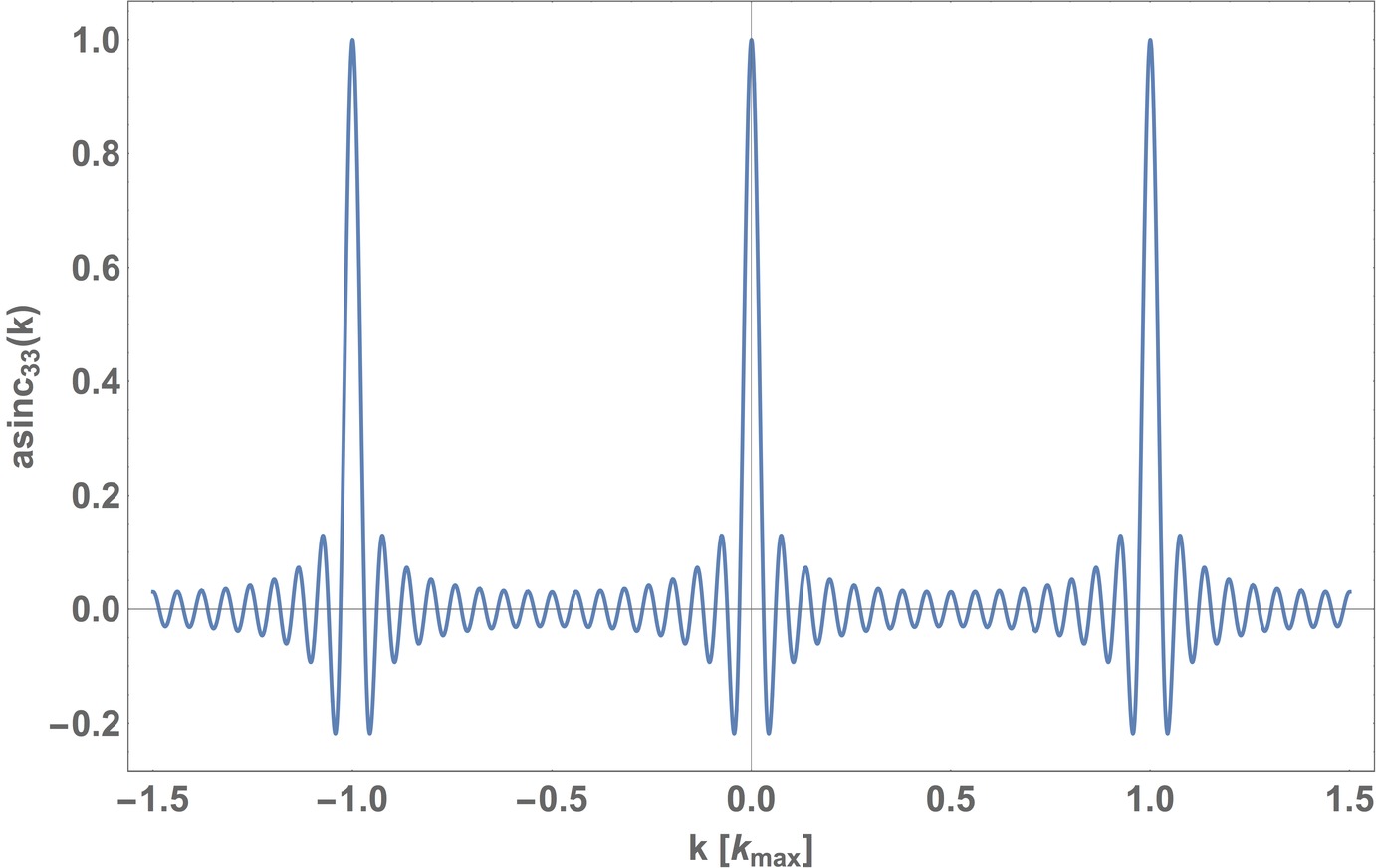
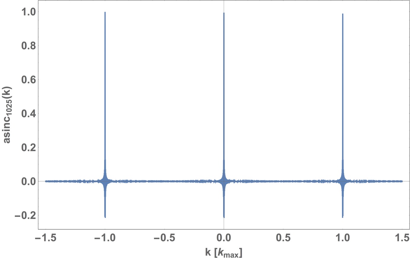
Figure II.9: The aliased $\operatorname{sinc}$ function with $\operatorname{asinc}_{M}(k)$ with $M=33$ and 1025 plotted in units of the sampling frequency of the grid $k_{max}$. Unlike the Dirac comb $\operatorname{asinc}_{M}(k)$ is non-local and oscillatory between the peaks, leading to distortions and aliasing effects even for band-limited signals. As is evident in the $M=1025$ case, both of these effects can be mitigated by using finer sampling grids since the width of the primary peaks at its base is $2/M$, and the value of the function at $k=k_{Ny}=k_{max}/2$ is $1/M$.

To derive this more rigorously we begin by denoting the FFT density grid in real space as

$$\delta_{n}^{f}(\mathbf{r})={}_{r}\left(\frac{\mathbf{r}}{H}\right)(\delta_{n}*W)(\mathbf{r})$$ (II.83)

where the superscript $f$ labels an FFT quantity and the subscript $n$ indicates sampling with discrete objects as before. This is equivalent to the statement that the $\delta_{n}^{f}(\mathbf{r})$ is a multiplication of the sampling grid, i.e. the Dirac comb ${}_{r}(\mathbf{r})=\sum_{\mathbf{r}_{g}}\delta_{D}(\mathbf{r}-\mathbf{r}_{g})=\sum_{\mathbf{n}}\delta_{D}(\mathbf{r}-H\mathbf{n})$ where $\mathbf{r}_{g}$ are the grid points and $\mathbf{n}\in\mathbb{Z}^{3}$ is a vector composed of integers, with the convolution between the density field sampled by discrete objects $\delta_{n}(\mathbf{r})$ and the window function $W(\mathbf{r})$ due to mass assignment. The Fourier Transform of this grid is $\delta_{n}^{f}(\mathbf{k})=\mathcal{F}[\delta^{f}_{n}(\mathbf{r})]$, but one should bear in mind that to obtain the FFT output one needs to further multiply this by the Dirac comb in $\mathbf{k}$-space, ${}_{k}(\mathbf{k})=\sum_{\mathbf{n}}\delta_{D}(\mathbf{k}-k_{F}\mathbf{n})$. The aliasing effects discussed in the previous paragraph becomes immediately apparent when one evaluates $\delta_{n}^{f}(\mathbf{k})$ explicitly which produces:

$$\delta_{n}^{f}(\mathbf{k})=\sum_{\mathbf{n}}\delta_{n}(\mathbf{k}-k_{max}\mathbf{n})W(\mathbf{k}-k_{max}\mathbf{n}).$$ (II.84)

This is merely a restatement of Figure II.6(b): sampling with a Dirac comb leads to aliased images spaced at intervals of $k_{max}$ in Fourier space. If the Nyquist criterion is satisfied, i.e. all frequencies in the signal satisfy $k<k_{max}/2=k_{Ny}$, then the images will not overlap and the signal remains undistorted (Figure II.7(a)). Otherwise aliasing artefacts will occur (Figure II.7(b)). The power spectrum we obtain via FFT, $P^{f}_{n}(k)$, is thus

$$P^{f}_{n}(k)=\sum_{\mathbf{n}}\left(P\left(\left|\mathbf{k}-k_{max}\mathbf{n}\right|\right)+\frac{1}{\bar{n}}\right)\left|W\left(\mathbf{k}-k_{max}\mathbf{n}\right)\right|^{2}$$ (II.85)

where we have included the effects of Poisson shot noise. We can see that the aliasing contributions are most prominent near the Nyquist frequency $k_{Ny}$ as was the case for the density field. Finally we note that to obtain the true FFT output one must multiply the expression in Equation II.85 by ${}_{f}\left(\frac{\mathbf{k}}{k_{F}}\right){}_{f}\left(\frac{\mathbf{-k}}{k_{F}}\right)={}_{f}\left(\frac{\mathbf{k}}{k_{F}}\right)$. The equivalent expression for the FFT bispectrum is

$$B^{f}_{n}(k_{1},k_{2},k_{3})$$

$$={} \sum_{\mathbf{n}_{1}\mathbf{n}_{2}}\Bigg{(}B\left(q_{1},q_{2},\left|\mathbf{q}_{1}+\mathbf{q}_{2}\right|\right)$$

$$\qquad+\frac{1}{\bar{n}}[P(q_{1})+P(q_{2})+P(\left|\mathbf{q}_{1}+\mathbf{q}_{2}\right|)]+\frac{1}{\bar{n}^{2}}\Bigg{)}$$

$$\quad\times W(\mathbf{q}_{1})W(\mathbf{q}_{2})W(-\mathbf{q}_{1}-\mathbf{q}_{2}),$$ (II.86)

where $\mathbf{q}_{i}=\mathbf{k}_{i}-k_{max}\mathbf{n}_{i}$, and the multiplicative factor that gives the true FFT output becomes

$${}_{f}\left(\frac{\mathbf{k}_{1}}{k_{F}}\right){}_{f}\left(\frac{\mathbf{k}_{2}}{k_{F}}\right){}_{f}\left(\frac{-\mathbf{k}_{1}-\mathbf{k}_{2}}{k_{F}}\right)$$

$$={} {}_{f}\left(\frac{\mathbf{k}_{1}}{k_{F}}\right){}_{f}\left(\frac{\mathbf{k}_{2}}{k_{F}}\right).$$ (II.87)

In principle this aliasing effect can be completely avoided by low-pass filtering the signal to remove the high-frequency contributions. This is equivalent to convolving the real-space signal with a $\operatorname{sinc}$ function (Jasche et al., 2009). However the $\operatorname{sinc}$ function is highly non-local and such an operation is computationally expensive since we would have to distribute all particles to every grid point. In addition we have assumed so far that our sampling operation in real space, i.e. ${}_{r}(\mathbf{r})$, has infinite extent, so that its Fourier transform is also an infinite Dirac comb. This cannot be achieved for practical reasons, and the Fourier transform of a truncated one-dimensional Dirac comb is the aliased $\operatorname{sinc}$ function $\operatorname{asinc}_{M}(k)$:

$$\mathcal{F}\left[\frac{1}{M}\sum_{n=-\frac{M-1}{2}}^{\frac{M-1}{2}}\delta_{D}(r-Hn)\right] =\frac{\sin(\pi kM/k_{max})}{M\sin(\pi k/k_{max})}$$

$$\equiv\operatorname{asinc}_{M}(k),$$ (II.88)

where we have introduced the normalisation factor $1/M$. We plot $\operatorname{asinc}_{M}(k)$ for $M=33$ and 1025 in Figure II.9, which correspond to sampling with FFT grids of size $32^{3}$ and $1024^{3}$ respectively. The aliased $\operatorname{sinc}$ function differ from the infinite Dirac comb in a very important way, i.e. its non-locality. When convolved with $\delta_{n}(\mathbf{r})$ the oscillatory features will distort the signal, and aliased images will always overlap even if the signal is band-limited. These aliasing contributions can be alleviated by low-pass filtering the signal, but one can not eradicate them nor uniquely restore the original signal (Jasche et al., 2009). However it should be noted that with sufficiently large $M$ one can typically neglect these contributions: the base width of the primary peaks is $2/M$ and the value of $\operatorname{asinc}_{M}(k)$ at the Nyquist frequency is $1/M$. Finally we remark that these finite, discrete sampling effects are exacerbated by the mass assignment procedure as the window function $W(\mathbf{k})$ also enters the aliased sum. This is a mild complication for the shot noise terms in Equations II.85 and II.86 as $W\left(\mathbf{k}-k_{max}\mathbf{n}\right)$ are typically simple analytical expressions (Jing, 2005). As for the product between the power spectrum and window function (Jing, 2005) proposed a procedure to cure these sampling effects iteratively by assuming the power spectrum $P(k)$ behaves like a power-law near the Nyquist frequency $k\sim k_{Ny}$. While this approximation seemed to work effectively for the power spectrum, it is not clear how one would similarly construct a simple analytical formula that captures the local behaviour of the bispectrum and higher order correlators effectively.

While no method has been found to fully recover the bispectrum near the Nyquist frequency, various solutions have been put forward to diminish the effects of aliasing. A straightforward approach is using higher order interpolation kernels such as PCS or Daubechies wavelets which are closer approximations to the ideal low-pass filter. In particular the authors of (Cui et al., 2008) claim that even with deconvolution of the corresponding window function, the power spectrum can be measured with the wavelets to an accuracy level of 2% in for wavenumbers up to $0.7k_{Ny}$. Since particle-mesh simulation codes rely on FFTs for rapid calculations of the gravitational potential, the Daubechies wavelets may prove useful as an inexpensive yet accurate way of representing particles on a grid. An alternative method is to push the aliasing effects to higher $k$ by first ‘supersampling’ the density field at some higher resolution than the one desired (Jasche et al., 2009). The super-sampled grid naturally has a higher Nyquist frequency thus we expect the aliasing effects at the target resolution to be much reduced. Finally we down-sample the super-sampled grid by deconvolving the relevant window function and removing all unwanted $k$-modes to obtain the signal sampled at the frequency of interest. The advantages of ‘supersampling’ over other methods are its effectiveness at removing undesirable aliasing distortions at the target frequency, and since low order mass assignment schemes such as CIC and TSC can be used for supersampling it is also computationally fast. However to super-sample at $n$ times the required resolution demands $n^{3}$ the amount of memory which can be a big limiting factor. A third method, propounded by (Sefusatti et al., 2016), sets out to remove the dominant aliasing contributions from odd images (cf. Figure II.7(b)) by interlacing two density grids that are shifted by half the grid spacing with respect to each other. The authors claim that the method, combined with a high order interpolation scheme such as PCS, can reduce systematic biases from aliasing to levels below 0.01% all the way up to the Nyquist frequency for both power spectra and bispectra estimates.

Investigation of these effects in the case opf the bispectrum is beyond the current scope of this paper and we leave it to future work. For the remainder of the paper we will instead avoid the issues mentioned above by simply limiting ourselves to $k<k_{max}/3=\frac{2}{3}k_{Ny}$.

III Results

III.1 Comparison between Dark Matter Simulation Codes

As we enter the age of precision cosmology we are ever more reliant on cosmological simulations to understand the dynamics of dark matter and baryons. Numerical simulations act as a buffer between theory and observation: we test cosmological models by matching simulation results to observational data, and hence obtain constraints on cosmological parameters. On the other hand since we only observe one universe we must turn to simulations to understand the statistical significance of our measurements. This is especially important with large galaxy data sets coming from current and near-future surveys such as DES, LSST, Euclid and DESI. While it would be ideal to use full N-body simulations to generate these so-called mock catalogues for statistical analysis, their huge demand for computational resources is prohibitive for generating the large number of simulations required for accurate estimates of covariances (Howlett et al., 2015). This has led to a proliferation of fast dark matter simulation tools, such as PINOCCHIO (Monaco et al., 2002, 2013), Quick Particle Mesh (QPM) (White et al., 2014), Augmented Lagrangian Perturbation Theory (ALPT) (Kitaura and Heß, 2013) and the Comoving Lagrangian Acceleration method (COLA) (Tassev et al., 2013). While the algorithms employed in all these methods are different, they all share the common aim of speeding up the simulation process at the expense of reduced accuracy at small scales.

These fast methods are typically bench-marked against N-body codes with the power spectrum and other two-point clustering statistics, as well as some form of three-point correlation, e.g. the reduced bispectrum

$$Q(k_{1},k_{2},k_{3})=\frac{B(k_{1},k_{2},k_{3})}{P(k_{1})P(k_{2})+P(k_{2})P(k_{3})+P(k_{3})P(k_{1})}$$ (III.1)

in some restricted domain. With MODAL-LSS we can incorporate full bispectrum estimation into the validation testing for these methods. The importance of these tests cannot be underestimated: the analysis in (Baldauf et al., 2016) has shown that theoretical and numerical uncertainties can strongly influence the extent to which observational data can be used to put constraints on cosmological parameters and hence possibilities of detecting new physics.

As a proof of concept we have elected to test the bispectra of three different fast dark matter methods, i.e. COLA, Particle-Mesh (PM) and second-order Lagrangian perturbation theory (2LPT) (Scoccimarro, 1998), against the Tree-PM N-body code GADGET-3 at various redshifts. L-PICOLA (Howlett et al., 2015; Scoccimarro et al., 2012) was used to generate the COLA, PM and 2LPT data due to its versatility and massively parallel performance, and its ability to generate and evolve the same 2LPT initial conditions used in our GADGET-3 runs. This means that all final outputs share the same initial seed and random phases, thus eliminating the need for cosmic variance considerations when comparing them.

III.1.1 Fast dark matter algorithms

Here we briefly summarise the three algorithms we test in this paper. For further details we refer the reader to relevant literature for 2LPT (Scoccimarro, 1998), PM (Hockney and Eastwood, 1988) and COLA (Howlett et al., 2015; Tassev et al., 2013).

2LPT

In Lagrangian perturbation theory (LPT) we track particles by their displacement $\bm{\psi}(\bm{q},t)$ from their initial position $\bm{q}$, i.e. $\bm{x}(t)=\bm{q}+\bm{\psi}(\bm{q},t)$, where $\bm{x}$ is the Eulerian position. First order in LPT leads to the well-known Zeldovich Approximation (ZA), which is particularly useful due to its analytical simplicity, and is often used to generate initial conditions for numerical simulations. However as shown in (Crocce et al., 2006a) 2LPT is a superior method at limited additional computational cost, and has since replaced ZA as the standard.

PM

The PM algorithm speeds up the calculation of gravitational forces though the use of a mesh: instead of summing all interactions between all the particles, we calculate the density field on a grid and use the Poisson equation to derive the gravitational potential in Fourier space. This computation is sped up greatly with FFTs, and it is straightforward to calculate the forces in real space at each grid point with the gradient of the potential and an inverse-FFT. The force on each particle is found by reversing the interpolation scheme used to place the particles on the grid. Here we use L-PICOLA’s implementation of the PM algorithm which is based on PMCODE (Klypin and Holtzman, 1997).

COLA

While the 2LPT produces excellent results at large scales, it quickly becomes deficient going into smaller scales as it fails to capture the full non-linearity of the system. The COLA algorithm is an efficient extension of 2LPT, boasting both speed and accuracy by trying to recover the residual Lagrangian displacement $\bm{\psi}_{res}$ between the 2LPT displacement and the full non-linear counterpart. The extra computations rely on variables already calculated and stored, such as the LPT and 2LPT displacements and the gravitational potential, the last of which is provided by the PM method.

III.1.2 Simulation Data

In order to probe a range of scales we have chosen two simulation box sizes of $1280\,h^{-1}$ Mpc and $640\,h^{-1}$ Mpc. The 2LPT Gaussian initial conditions were generated using L-PICOLA at redshift $z_{i}=99$ to ensure the suppression of transients in power spectra and bispectra estimates of our simulations (McCullagh et al., 2016), with an input linear power spectrum at redshift $z=0$ produced by CAMB (Lewis et al., 2000). A PM grid size of $2048^{3}$ was then used to evolve the $2048^{3}$ particles in each run where applicable. The fiducial cosmology is flat $\Lambda$CDM with extended Planck 2015 cosmological parameters (TT,TE,EE+lowP+lensing+ext, see Table III.1). The expensive GADGET-3 run was completed on the COSMA facility at Durham while the other codes and all subsequent analysis was finished with the COSMOS supercomputer at Cambridge. The small deviations in output redshifts between GADGET-3 and L-PICOLA were corrected with the appropriate linear growth factor

$$D_{1}(a)=\frac{E(a)}{D_{1,0}}\int^{a}_{0}\frac{da^{\prime}}{a^{\prime 3}E^{3}(a^{\prime})}$$ (III.2)

where

$$E(a)=\frac{H(a)}{H_{0}}=\sqrt{\Omega_{m}a^{-3}+\Omega_{\Lambda}}$$ (III.3)

for a flat cosmology, and

$$D_{1,0}=\int^{1}_{0}\frac{da^{\prime}}{a^{\prime 3}E^{3}(a^{\prime})}$$ (III.4)

is introduced to normalise $D_{1}(z=0)=1$.

Description	Symbol	Value
Hubble constant	$H_{0}$	67.74 $\text{km}\,\text{s}^{-1}$
Physical baryon density parameter	$\Omega_{b}h^{2}$	0.02230
Matter density parameter	$\Omega_{m}$	0.3089
Dark energy density parameter	$\Omega_{\Lambda}$	0.6911
Fluctuation amplitude at $8h^{-1}$ Mpc	$\sigma_{8}$	0.8196
Scalar spectral index	$n_{s}$	0.9667
Primordial amplitude	$10^{9}A_{s}$	2.142

(a) Planck 2015 cosmological parameters (rightmost column of Table 4 in (Planck Collaboration, 2016a))

Description	Symbol	Value
Physical neutrino density parameter	$\Omega_{\nu}h^{2}$	0.000642
Number of effective neutrino species	$N_{eff}$	3.046
Curvature density parameter	$\Omega_{k}$	0.0000

(b) Extensions to base $\Lambda$CDM parameters (rightmost column of Table 5 in (Planck Collaboration, 2016a))

Table III.1: For consistency between the Planck parameters and the CAMB output we incorporated one massive neutrino species with a small energy density. The lack of radiation and neutrino evolution in L-PICOLA and GADGET-3 has led us to define the matter power spectrum to consist only of cold dark matter and baryons, hence the raised value of $\sigma_{8}$ instead of the Planck value of 0.8159. The pivot scale for $n_{s}$ is 0.05 $\text{Mpc}^{-1}$.

In addition to Table III.1, the following are the key parameters we used to generate the initial power spectrum and evolve the initial conditions:

CAMB

We use only cold dark matter (CDM) and baryons to define the matter power spectrum and $\sigma_{8}$, i.e. transfer_power_var = 8. The relevant neutrino parameters are massless_neutrinos = 2.046 and massive_neutrinos = 1.

L-PICOLA

Three different logarithmic time steppings in $a$ were used to test the accuracy of COLA: $\Delta(\ln a)=0.01$ (the same time-stepping we use for GADGET-3), 0.046 and 0.23. They correspond to 460, 100 and 20 time-steps from $z=99$ to $z=0$ respectively.

GADGET-3

We used (McCullagh et al., 2016; Crocce et al., 2006b) as guides in setting the parameters to ensure high numerical accuracy in our simulations: MaxRMSDisplacementFac = 0.1, ErrTolIntAccuracy = 0.01, MaxSizeTimestep = 0.01, ErrTolTheta = 0.2 and ErrTolForceAcc = 0.002. A smoothing length of $0.05L/N$ where $L$ is the simulation box size and $N=2048$ is the number of particles per dimension was used.

III.1.3 Simulation Power Spectra

Figure III.1: Ratio between the power spectra of the various fast dark matter codes and GADGET-3 for the 2 simulation boxes. All the power spectrum estimates were performed with GADGET-3. The sub-par performance of 2LPT and COLA with a coarse time-stepping of $\Delta(\ln a)=0.23$ is unsurprising, but the $\Delta(\ln a)_{0.046}$ COLA simulation with compares quite favourably with PM and the $\Delta(\ln a)_{0.01}$ COLA with at a fraction of the computational cost. As noted by its authors the ability to reproduce the matter power spectrum at a reasonable accuracy but with reduced computational resources compared to conventional PM methods is the strength of the COLA method (Howlett et al., 2015).

We estimated the power spectra of our simulations with GADGET-3. To minimise errors coming from aliasing effects the power spectra of each simulation was estimated three times: once with a $2048^{3}$ PM grid and two further times by ‘folding’ (Colombi et al., 2009) that grid onto itself by factors of 2 and 4 respectively. The disadvantage of this folding method is the reduction in the number of modes at large scales leading to greater cosmic variance. We therefore combine these three power spectra together to guarantee precision over the entire $k$-ranges considered here. We did not observe shot noise in the power spectra of the initial conditions, and due to large number densities used did not find it necessary to correct for shot noise in the simulation outputs (cf. Equation II.64).

Figure III.1 shows the ratio between the power spectra of the fast codes and GADGET-3 at redshift $z=0.5$. While 2LPT and $\Delta(\ln a)_{0.23}$ COLA compare poorly to GADGET-3 as expected, the power of the COLA algorithm to imitate the performance of PM in fewer time-steps is shown by the $\Delta(\ln a)_{0.046}$ case. It should be noted that PM does perform slightly better than COLA when the same number of time-steps are used.

III.1.4 Simulation Bispectra

(a) Redshift $z=9$

(b) Redshift $z=3$

(c) Redshift $z=2$

(d) Redshift $z=1$

(e) Redshift $z=0.5$

(f) Redshift $z=0$

Figure III.2: Redshift evolution of the estimated bispectra from a $1280\,h^{-1}$ Mpc GADGET-3 simulation, plotted up to $k_{max}=2.0\,h\,\text{Mpc}^{-1}$. This shows clearly how the flattened tree-level signal dominates the early time bispectra, but the constant shape brought about by the aggregation of matter takes over at late times. To emphasise this point we have scaled the maxima of the colour bars for redshifts $z=3\rightarrow 0$ relative to redshift $z=9$ by the appropriate linear growth factor, $D_{1}(z)/D_{1}(z=9)$. The SN-weighted tree-level bispectrum grows as $D_{1}(z)$, and the saturation of the signal for redshifts $z=1,0.5,0$ demonstrate faster growth than that dictated by perturbation theory in the non-linear regime. It is remarkable that the only shape generated by the collapse of dark matter into halos is the constant shape. Therefore after $z~{}2$ we observe a steady growth in the strength of the signal but very little change in the bispectrum morphology.

(a) 2LPT

(b) $\Delta(\ln a)_{0.23}$ COLA

(c) $\Delta(\ln a)_{0.01}$ COLA

(d) $\Delta(\ln a)_{0.046}$ COLA

(e) PM

(f) Boosted $\Delta(\ln a)_{0.01}$ COLA

Figure III.3: Bispectrum residuals at redshift $z=0.5$ between the $1280\,h^{-1}$ Mpc fast dark matter and GADGET-3 simulations, plotted up to $k_{max}=2.0\,h\,\text{Mpc}^{-1}$. The lack of non-linear signal in the fast dark matter simulations is evident, leading to a deficient constant shape in their bispectra.

The density field of the simulations were first obtained via a CIC mass assignment. A smoothed GADGET-3 power spectrum at the appropriate redshifts were used in the signal-to-noise weighting of the bispectrum (Equation II.33).

In Figure III.2 we show the estimated bispectra for the $1280\,h^{-1}$ Mpc GADGET-3 simulations described in Section III.1.2 up to $k_{max}=2.0\,h\,\text{Mpc}^{-1}$. We choose this resolution to best highlight the transition from the tree-level dominant signal seen in early redshifts to the strong constant shape presence induced by non-linear gravitational evolution at late times. In particular we see that this happens most prominently from redshift $z=3$, where there is still some competition between the flattened and equilateral signals, to redshift $z=2$, in which the constant shape has taken over. This is one of the many advantages of estimating the full bispectrum, as its morphology typically offers unique information regarding structure formation that cannot be gained from the power spectrum. Another point of note is that the formation of dark matter halos through virialisation generates only one bispectrum shape which is the constant shape, as evidenced by the lack of change in the bispectrum past $z=2$ bar a growth in signal strength. We also show the bispectrum residuals between the fast dark matter codes and GADGET-3 in Figure III.3. The inability of the fast codes to resolve small scale structure is illustrated by the lack of constant shape signal in their bispectra. These pictures agrees qualitatively with the power spectra results in Figure III.1.

To make quantitative comparisons we invoke the correlators introduced in Section II.3.1. The $f_{nl}$ correlators of the fast dark matter codes with GADGET-3:

$$f_{nl}(\hat{B}_{\text{DM}},\hat{B}_{\texttt{GADGET-3}{}}) =\frac{\sum_{n}\beta^{R}_{\text{DM},n}\beta^{R}_{\texttt{GADGET-3}{},n}}{\sum_{n}(\beta^{R}_{\texttt{GADGET-3}{},n})^{2}}$$ (III.6)

are shown in Figure III.4; we do not plot the shape correlators as they only provide redundant information. The first thing to note is a striking resemblance to the power spectra plots in Figure III.1, as the power spectrum enters the $f_{nl}$ correlator through the weighted inner products between bispectra (Equation II.32). Since we use the GADGET-3 power spectrum for the weighting, bispectra comparisons will inevitably be biased by the lack of power in the fast dark matter power spectra. To address this issue and show the differences due to the bispectrum alone we propose boosting the power spectrum of the fast code in Fourier space:

$$\delta_{\text{DM}}(\mathbf{k})\rightarrow\sqrt{\frac{\hat{P}_{\texttt{GADGET-3}{}}(k)}{\hat{P}_{\text{DM}}(k)}}\delta_{\text{DM}}(\mathbf{k}).$$ (III.7)

The residuals between the boosted $1280\,h^{-1}$ Mpc $\Delta(\ln a)_{0.01}$ COLA simulation and GADGET-3 is shown in Figure III.3, demonstrating more than a 3x reduction in magnitude compared to the unboosted COLA and PM runs. More quantitatively the boosted $\Delta(\ln a)_{0.01}$ COLA bispectra also show much improved $f_{nl}$ correlation with GADGET-3 as seen in Figure III.4. We therefore conclude this is an effective yet relatively inexpensive method to improve the performance of fast simulation codes. Nevertheless a dip in correlation at small scales remain after boosting which reflects that there is bispectrum information lost which is independent of the power spectrum.

(a)

(b)

Figure III.4: $f_{nl}$ correlators between the bispectra of fast dark matter codes and GADGET-3. The similarities of these plots to those in Figure III.1 is due to the power spectrum weighting present in inner products between bispectra (Equation II.32), thus a mismatch in power spectra naturally leads to discrepancies in bispectrum comparisons. This may suggest that the differences we see here are due to the power spectrum alone, but clearly this is not the case since the ‘boosted’ COLA simulation has an identical power spectrum to GADGET-3 yet still suffers from a lack of bispectrum signal at small scales. However, the improved performance of the boosted COLA bispectrum demonstrates the effectiveness of the ‘boosting’ method.

III.2 Gaussian vs Non-Gaussian covariances

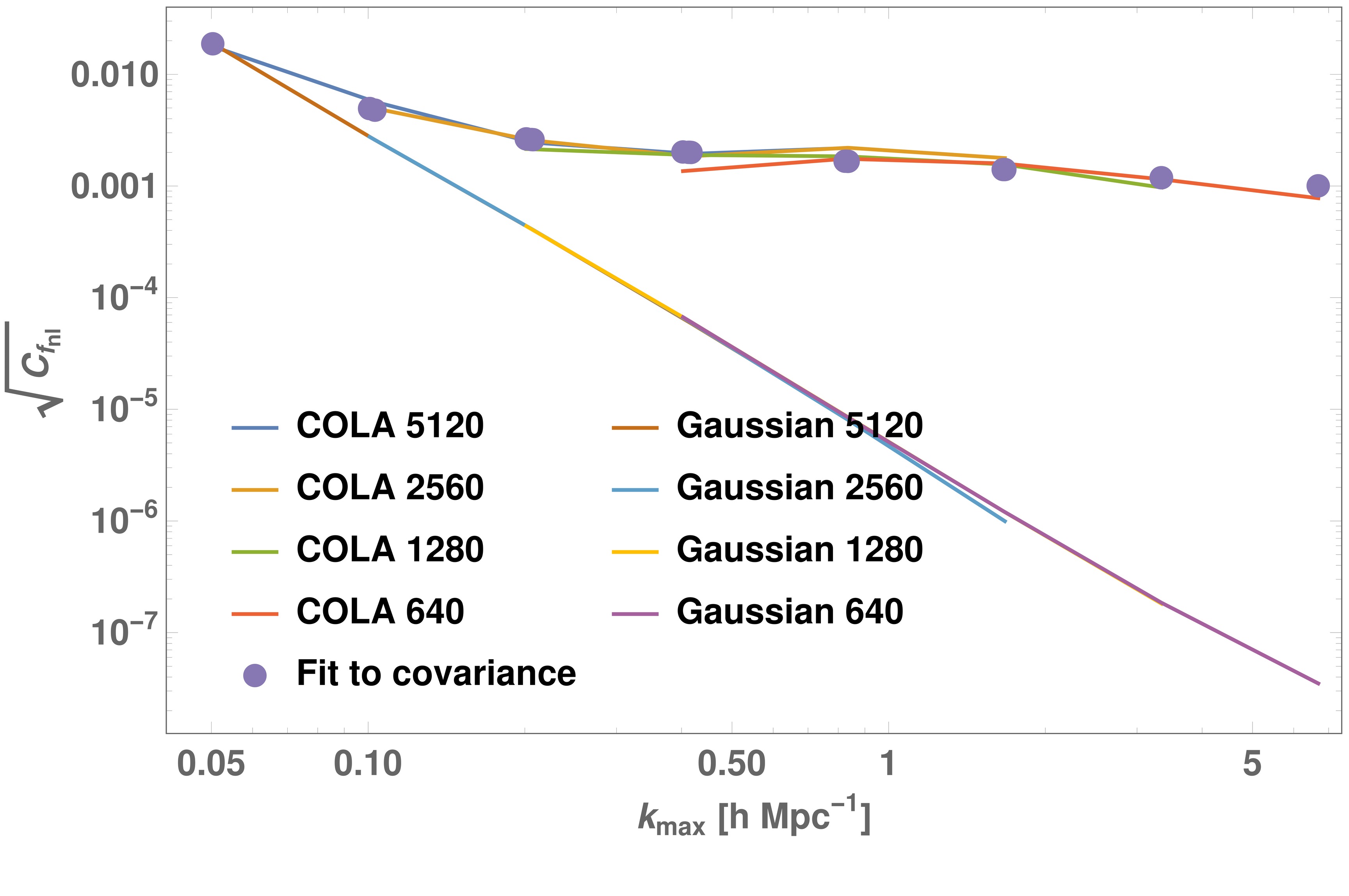
Figure III.5: The full covariance of the $f_{nl}$ correlator estimated using 10 COLA runs compared to the Gaussian contribution calculated using Equation II.77 with the 3-shape model. The two begin to diverge significantly at $k\sim 0.1\,h\,\text{Mpc}^{-1}$, signalling the dominance of non-Gaussian covariances. Since the covariance scales inversely as the cube of the box size, in order to combine the estimates from the different simulations we have re-scaled them accordingly against the $5120\,h^{-1}$ Mpc runs. The purple points are the best-fit to the full covariance with the function $f=Ak^{-a}+Bk^{-b}$ and the parameters $A=3.2477\times 10^{-6},B=1.5871\times 10^{-3},a=2.8339,b=0.2409$.

The extent to which we can put constraints on cosmological parameters through the bispectrum is dependent on the covariance of MODAL-LSS estimator. To find the full covariance we first average over 10 boosted COLA realisations for an estimate of the mean bispectrum $\bar{\beta}$, then calculate the variance in $f_{nl}(\beta,\bar{\beta})$ as an estimate for $C_{f_{nl}}$ (Equation II.77). The computational cost of COLA runs are sufficiently low that additional to the $1280\,h^{-1}$ Mpc and $640\,h^{-1}$ Mpc boxes we have also completed runs with $5120\,h^{-1}$ Mpc and $2560\,h^{-1}$ Mpc box sizes, so that we can explore the regime where Gaussian covariances dominate. We have made a least-squares fit of the full covariance $\sqrt{C_{f_{nl}}}$ with the curve_fit algorithm in Scipy, using the default Levenberg-Marquardt method (Moré, 1978). We model the full covariance a sum of two power laws: $f=Ak^{-a}+Bk^{-b}$, which represents the Gaussian and non-Gaussian contributions respectively. The best-fit is obtained using the following values for these parameters: $A=4.6480\times 10^{-6},B=1.0900\times 10^{-3},a=2.5978,b=0.2315$.

Our estimates are shown in Figure III.5 where we also plot the Gaussian covariances calculated using Equation II.77 with the 3-shape model $\alpha^{R}_{n}$ coefficients. It is clear that while the Gaussian covariance continues to diminish in the non-linear regime due to more modes being available, the non-Gaussian covariance starts to dominate at $k\sim 0.1\,h\,\text{Mpc}^{-1}$ and then asymptotes towards$\sim 0.1\%$. This has important consequences on e.g. Fisher matrix forecasts, especially if non-Gaussian covariances are not taken in account which could strongly skew theoretical error estimates. While the combination of power spectrum and bispectrum is superior to using the power spectrum alone, the improvement may not be as significant as one might have hoped due to this plateauing in the bispectrum covariance.

III.3 Comparison between Dark Matter Simulations and Theory

(a) 10000 averaged $256^{3}$ COLA runs

(b) 10 averaged $512^{3}$ COLA runs

(c) 10 averaged $1024^{3}$ COLA runs

(d) 10 averaged $2048^{3}$ COLA runs

(e) Tree-level bispectrum

Figure III.6: The reconstructed bispectra from averaged 2LPT IC, and the desired signal, i.e. the tree-level bispectrum, plotted up to $k_{max}=0.41\,h\,\text{Mpc}^{-1}$ . The colour scale is chosen to show the full range of the tree-level bispectrum, leading to significant saturation for the simulation bispectra. With increeasing FFT grid size the IC bispectrum morphology approaches the theoretical one, but the amplitude remains grossly inflated.

The development of the MODAL-LSS toolkit is to allow straightforward comparisons between bispectra, either from simulations, observational data, or theory. In that cause we first test our method by estimating the bispectrum of 2LPT initial conditions (IC) generated by L-PICOLA, using the fact that it should reproduce the tree-level bispectrum. We used a range of grid sizes to generate the initial conditions, and to combat cosmic variance at large scales we average over multiple realisations. Similar to the test in Section II.4.3 we use Equations II.34 and II.29 to find that

$$\mathcal{S}_{\beta,\alpha} =\frac{\sum_{n}\beta^{R}_{n}\alpha^{R}_{n}}{\sqrt{\sum_{n}(\beta^{R}_{n})^{2}\sum_{n}(\alpha^{R}_{n})^{2}}},$$

$$f_{nl}^{\beta,\alpha} =\frac{\sum_{n}\beta^{R}_{n}\alpha^{R}_{n}}{\sum_{n}(\alpha^{R}_{n})^{2}}.$$ (III.8)

The correlators between the averaged runs and the tree-level bispectrum are shown in Table III.2, and we also plot the reconstructed simulation bispectra in Figure III.6.

$k_{max}\,(h\,\text{Mpc}^{-1})$	10000 averaged $256^{3}$ runs		10 averaged $512^{3}$ runs		10 averaged $1024^{3}$ runs		10 averaged $2048^{3}$ runs
	$\mathcal{S}_{\beta,\alpha}$	$f_{nl}^{\beta,\alpha}$	$\mathcal{S}_{\beta,\alpha}$	$f_{nl}^{\beta,\alpha}$	$\mathcal{S}_{\beta,\alpha}$	$f_{nl}^{\beta,\alpha}$	$\mathcal{S}_{\beta,\alpha}$	$f_{nl}^{\beta,\alpha}$
0.4123	0.9300	11.12	0.9339	5.603	0.9469	3.072	0.9583	1.830
0.8296	-	-	0.9501	6.076	0.9613	3.228	0.9794	1.895
1.6690	-	-	-	-	0.9696	3.442	0.9830	1.950
3.3429	-	-	-	-	-	-	0.9870	2.064

Table III.2: Comparisons between averaged 2LPT IC bispectra and the tree-level bispectrum, where the IC have been generated with different grid sizes. The poor shape correlation at low $k$ cannot be caused by cosmic variance alone due to the high number of runs used, and a clear trend of scale dependence can be seen in the $f_{nl}$ correlator.

The poor shape correlation ($<95\%$) for low $k$ is a strong indication that something is wrong with the IC, but cosmic variance cannot be the only source of error since a very large number of runs were used in the $256^{3}$ case. We have also ruled out shot noise since it is not the correct shape. Moreover the large amplitude of the simulation bispectra leads to an inflated $f_{nl}$ in a way that is dependent on the size of the FFT grid used. We propose this failure of the IC code to reproduce the correct bispectrum is due to both (i) transients, as discussed in (McCullagh et al., 2016; Uhlemann et al., 2018), and (ii) grid effects. Similar problems were observed in (Schmittfull et al., 2013b), and subsequently alleviated by the use of glass initial conditions. With more sophisticated technology at hand now we shall investigate this further in the near future.

(a) Shape correlator

(b) $f_{nl}$ correlator

Figure III.7: Correlators between a $1280\,h^{-1}$ Mpc GADGET-3 simulation and the tree-level bispectrum at various redshifts. Transients is the likely suspect for the especially poor shape correlation at low $k$ at redshift $z=9$.

Another obvious candidate for our tests is the redshift evolution of a simulation. It is natural to expect a faithful adherence to the tree-level bispectrum at earlier times, even at high $k$. With the passage of time, and hence gravitational collapse, the non-linear signal will eventually dominate at small scales, leading to significant deviations from perturbation theory. This is shown clearly in Figure III.7, where we compare the $1280\,h^{-1}$ Mpc GADGET-3 simulation to the tree-level bispectrum. As the smallest FFT grid we use in bispectrum estimation is $256^{3}$ we unfortunately miss out on the observationally relevant scales of $k\sim 0.1\,h\,\text{Mpc}^{-1}$, but our efforts to recover the tree-level bispectrum in larger simulations (i.e. 1280 and $2560\,h^{-1}$ Mpc) have failed, probably due to the same issues we encountered when we tried to extract the initial conditions bispectra. Transients are the most likely explanation for the poor shape correlation at low $k$, especially at redshift $z=9$, as the correlation improves with time when these modes decay away.

IV Conclusions

In this paper we present the newly improved MODAL-LSS code for efficiently computing the bispectrum of any 3D input density field. This code enables us to do high precision analysis with the dark matter bispectrum from large N-body simulations or faster alternative codes, and to make detailed quantitative comparisons between theory and simulations. By exploiting highly optimised numerical libraries, we were able to incorporate 1000 separable modes in the bispectrum analysis (relative to 50 modes previously (Schmittfull et al., 2013a)), also including specially tailored modes to accurately recover the tree-level bispectrum. This allows convergence to a much broader range of nonlinear gravitational and primordial bispectra and makes generic non-Gaussian searches feasible in huge future galaxy surveys.

First, we have addressed a few common areas where errors in the MODAL-LSS estimator can be significant, i.e. shot noise, the covariance of the estimator, and aliasing effects from using FFTs. Shot noise in the bispectrum is well-known and required little discussion. The full covariance of the MODAL-LSS estimator was derived for the first time, but the non-Gaussian contributions to the covariance appear to be analytically intractable, even with the separable modal expansion, so we can only estimate the Gaussian covariance, and we must tackle the problem numerically. While others have investigated of discrete FFT methods on bispectrum estimation, we find that contrary to other estimators the MODAL-LSS estimator breaks down at the same frequency as power spectra estimators, i.e. at the Nyquist frequency $k_{Ny}$, rather than at $\frac{2}{3}k_{Ny}$. We believe this is not a consequence of the MODAL-LSS method but rather a general result in bispectrum estimation since the aliasing effects come from the discrete sampling of the density field and not the use of FFTs itself.

With many large galaxy data-sets on the horizon, there is a pressing need for fast mock catalogue codes. While these fast codes are designed to only replicate the accuracy of N-body codes at large scales without resolving finer structure, we have found a simple and effective way to enhance their performance. A comparison between the 2LPT, PM and COLA algorithms against GADGET-3 shows 2LPT is deficient in both the power spectrum and bispectrum, while the COLA algorithm is successful in giving comparable performance to PM with fewer time-steps. Noting that the drop in bispectrum at large scales might be influenced by the power spectrum, we attempted to rectify this by boosting the power spectrum of the COLA simulation and saw a significant reduction in the power lost.

Finally we address the theoretical modelling of the dark matter bispectrum by examining the full covariance of the MODAL-LSS estimator, showing that non-Gaussian contributions begin to dominate at $k\sim 0.1\,h\,\text{Mpc}^{-1}$ and plateaus towards $\sim 0.1\%$. This is a significant adjustment as the non-Gaussian covariance is difficult to calculate even numerically, leading to the use of only the Gaussian covariance in most Fisher matrix forecasts. In principle, this will lead to gross underestimates of the theoretical error and thus the ability to put constraints on cosmological parameters. To show the power of the MODAL-LSS method in testing theoretical models against simulations we have compared (i) 2LPT initial conditions against the tree-level bispectrum, and (ii) a GADGET-3 simulation against the tree-level bispectrum at various redshifts. We have observed problematic transient modes and grid effects that affect the initial conditions, where the tree-level bispectrum should be recovered after averaging over many realisations. These effects propagate and persist to late times on the largest scales, as shown in a GADGET-3 comparison, and must be addressed in the initial conditions.

V Acknowledgements

We are especially grateful to Tobias Baldauf for many enlightening conversations and for his frequent useful advice. We are also very grateful for discussions with Marc Manera and Marcel Schimmittfull, who pioneered the first MODAL approach to the LSS bispectrum (Schmittfull et al., 2013a). Kacper Kornet and Juha Jaykka provided invaluable technical support for MODAL-LSS code optimisation and dealing with this large in-memory pipeline. JRF and EPS acknowledge support from STFC Consolidated Grant ST/P000673/1.

This work was undertaken on the COSMOS Shared Memory system at DAMTP, University of Cambridge operated on behalf of the STFC DiRAC HPC Facility. This equipment is funded by BIS National E-infrastructure capital grant ST/J005673/1 and STFC grants ST/H008586/1, ST/K00333X/1.

This work used the COSMA Data Centric system at Durham University, operated by the Institute for Computational Cosmology on behalf of the STFC DiRAC HPC Facility (www.dirac.ac.uk). This equipment was funded by a BIS National E-infrastructure capital grant ST/K00042X/1, DiRAC Operations grant ST/K003267/1 and Durham University. DiRAC is part of the National E-Infrastructure.

Appendix A Calculation of $\gamma_{nm}$ with FFTs

(a) $\gamma_{nm}$ calculated directly on the tetrapyd for 1000 shifted Legendre polynomials using 42 grid points in each dimension. The abundance of off-diagonal features demonstrate the lack of orthogonality between modes on the tetrapyd, especially for high $n$.

(b) The same calculation but using FFTs over $128^{3}$ grids in real space, but keeping the same $k_{max}$. While this qualitatively agrees with the plot to the left, the off-diagonal elements differ wildly quantitatively, demonstrating much stronger orthogonality between the modes.

Figure A.1: To better highlight the off-diagonal structure, in both of these figures we plot $\log_{10}\left|\frac{\gamma_{nm}}{\sqrt{\gamma_{nn}\gamma_{mm}}}\times 10^{6}\right|$, such that the diagonal is always 6, and limit the plot range to $[0,6]$. This is important since we need the inverse of $\gamma_{nm}$ to rotate the MODAL-LSS coefficients in the $Q$ basis to the $R$ basis, and even small numerical differences in the off-diagonal elements can create large deviations in the final result.

As mentioned in the main text the integral

$$\gamma_{nm}\equiv\frac{V}{\pi}\int_{\mathcal{V}_{B}}dV_{k}Q_{n}Q_{m}$$ (A.1)

can be evaluated in two ways. The first is by direct integration on the tetrapydal domain which gives the most accurate answer. In Figure A.1(a) we show $\gamma_{nm}$ calculated in this way for 1000 modes using shifted Legendre polynomials and 42 grid points in each dimension.

Alternatively this can be done with the use of FFTs. It can be shown that for any function $F(k_{1},k_{2},k_{3})$ this expression holds:

$$\int\frac{d^{3}k_{1}}{(2\pi)^{3}}\frac{d^{3}k_{2}}{(2\pi)^{3}}\frac{d^{3}k_{3}}{(2\pi)^{3}}(2\pi)^{6}\delta^{2}_{D}\left(\mathbf{k}_{1}+\mathbf{k}_{2}+\mathbf{k}_{3}\right)F$$

$$\quad=\frac{V}{8\pi^{4}}\int_{\mathcal{V}_{B}}dk_{1}dk_{2}dk_{3}\,k_{1}k_{2}k_{3}F.$$ (A.2)

Therefore we can write down an expression for $\gamma_{nm}$ in terms of inverse Fourier Transforms:

$$\gamma_{nm}$$

$$=(2\pi)^{9}\int_{\mathbf{k}_{1},\mathbf{k}_{2},\mathbf{k}_{3}}\delta_{D}(\mathbf{k}_{1}+\mathbf{k}_{2}+\mathbf{k}_{3})\frac{Q_{n}Q_{m}}{k_{1}k_{2}k_{3}}$$

$$=(2\pi)^{6}\int d^{3}x\int\frac{\prod_{i}d^{3}k_{i}}{(2\pi)^{9}}e^{i(\mathbf{k}_{1}+\mathbf{k}_{2}+\mathbf{k}_{3})\cdot\mathbf{x}}\frac{Q_{n}Q_{m}}{k_{1}k_{2}k_{3}}$$

$$=\frac{(2\pi)^{6}}{6}\int\left[M_{r_{1}r_{2}}(\mathbf{x})M_{s_{1}s_{2}}(\mathbf{x})M_{t_{1}t_{2}}(\mathbf{x})+5\,\text{perms}\right]d^{3}x,$$ (A.3)

where we have suppressed the arguments $(\frac{k_{1}}{k_{max}},\frac{k_{2}}{k_{max}},\frac{k_{3}}{k_{max}})$ of $Q_{n}$ and $Q_{m}$ for brevity, and introduce the integrals

$$M_{r_{1}r_{2}}(\mathbf{x})=\int\frac{d^{3}k}{(2\pi)^{3}}\frac{1}{k}q_{r_{1}}(k/k_{max})q_{r_{2}}(k/k_{max})e^{i\mathbf{k}\cdot\mathbf{x}}$$ (A.4)

resulting from the product $Q_{n}Q_{m}$. For $n\equiv\{r_{1},s_{1},t_{1}\}$ and $m\equiv\{r_{2},s_{2},t_{2}\}$ this product produces 36 terms, but only 6 unique combinations, i.e.

• $(r_{1}r_{2})(s_{1}s_{2})(t_{1}t_{2})$

• $(r_{1}s_{2})(s_{1}t_{2})(t_{1}r_{2})$

• $(r_{1}t_{2})(s_{1}r_{2})(t_{1}s_{2})$

• $(r_{1}r_{2})(s_{1}t_{2})(t_{1}s_{2})$

• $(r_{1}s_{2})(s_{1}r_{2})(t_{1}t_{2})$

• $(r_{1}t_{2})(s_{1}s_{2})(t_{1}r_{2})$,

hence the 6 permutations in the final line of Appendix A. Figure A.1(b) shows the result of such a calculation with $128^{3}$ grids in real space, but keeping the same $k_{max}$. The discrepancy in number of grid points arises from aliasing considerations when putting particles on a grid, as discussed in Section II.5.3. Although this is not relevant here we only use up to $\frac{2}{3}k_{Ny}$ of FFT grids here for consistency with our analysis of simulation data. Thus, both methods effectively use the same number of grid points as far as the tetrapyd is concerned.

Although Figure A.1(a) and Figure A.1(b) share qualitatively similarities, demonstrating the same grid structure and features along the main diagonal and its close neighbours, the numerical values of the off-diagonal elements are much smaller with the FFT calculation. Curiously this would suggest the modes are more orthogonal to each other when used in conjunction with FFTs. In rotating the MODAL-LSS coefficients from the $Q$ to $R$ basis we need to calculate $\lambda_{nm}$ (Equation II.56), given by $\gamma^{-1}=\lambda^{T}\lambda$. Since the inverse of a matrix is highly susceptible even to small changes in off-diagonal elements, big differences in the final bispectrum estimation can result if one is not careful. To illustrate this effect we made the following tests of the FFT-based MODAL-LSS code using randomly generated Gaussian density fields. Gaussianity implies the lack of bispectrum and higher order correlators, which has two consequences on the MODAL-LSS coefficients. First, $\expectationvalue{\beta^{Q}_{n}}=\langle\beta^{R}_{n}\rangle=0$ due to the absence of any bispectrum. Additionally, as shown in the MODAL-LSS covariance calculation (Equation II.74), for a Gaussian density field the $\beta^{Q}$ coefficients satisfy $\expectationvalue{\beta^{Q}_{m}\beta^{Q}_{n}}=\gamma_{mn}$. To ensure the internal consistency of the method we rotate this expression into the $R$ basis with the $\gamma_{nm}$ calculated with the two methods above and check if we recover $\expectationvalue{\beta^{R}_{m}\beta^{R}_{n}}=\delta_{mn}$. The conversion is achieved in the same manner as discussed in Section II.4.2 by first taking the Cholesky decomposition of $\gamma$ to obtain $\lambda^{-1}$, then a further matrix inversion gives $\lambda$. These are good sanity checks that our numerical code is behaving as expected and that the algorithm does indeed work.

The results of the $\langle\beta^{R}_{n}\rangle=0$ test is shown in Figure A.2 and the $\expectationvalue{\beta^{R}_{n}\beta^{R}_{n}}=1$ test in Figure A.3. Here we used $128^{3}$ FFT grids and 42 tetrapyd points as above. The $\langle\beta^{R}_{n}\rangle=0$ test is inconclusive as $\langle\beta^{R}_{n}\rangle$ calculated both ways are consistent with 0, but when the $\gamma_{nm}$ calculated with the tetrapyd is used a strong divergence from the mean is observed at high $n$, which might be an indication that something is amiss. On the other hand Figure A.3 clearly demonstrates the problem with using the tetrapyd-based $\gamma_{nm}$, as even stronger deviations are seen due to the inconsistent off-diagonal terms. We conclude that if the incorrect $\gamma_{nm}$ is used one would not bias the mean (i.e. the bispectrum estimation itself), but would lead to hugely inflated covariances in the estimated bispectrum.

(a) $\gamma_{nm}$ calculated on the tetrapyd, giving $\langle\beta^{R}_{n}\rangle=0.016\pm 0.202$. Although this is consistent with 0, it is clear the higher modes are strongly divergent from the mean which is an indication something is wrong.

(b) $\gamma_{nm}$ calculated with FFTs, giving $\langle\beta^{R}_{n}\rangle=0.0001\pm 0.0048$. It is clear the $\beta^{R}_{n}$ thus obtained is much better behaved across the entire range of $n$, without any of the divergences seen to the left.

Figure A.2: Testing the $\gamma_{mn}$ matrices by rotating $\beta^{Q}_{n}$ into $\beta^{R}_{n}$ and checking $\langle\beta^{R}_{n}\rangle=0$.

(a) $\gamma_{nm}$ calculated on the tetrapyd, giving $\expectationvalue{\beta^{R}_{n}\beta^{R}_{n}}=4000\pm 22000$. There is no doubt that using this $\gamma_{nm}$ will lead to inconsistent bispectrum estimates.

(b) $\gamma_{nm}$ calculated with FFTs, giving $\expectationvalue{\beta^{R}_{n}\beta^{R}_{n}}=0.997\pm 0.045$. This gives the correct mean and the correct order of magnitude in error since $\frac{1}{\sqrt{1000}}\sim 3.3\%$.

Figure A.3: Testing the $\gamma_{mn}$ matrices by checking $\expectationvalue{\beta^{R}_{n}\beta^{R}_{n}}=1$.

(a) 341 grid points, giving $\expectationvalue{\beta^{R}_{n}\beta^{R}_{n}}=0.960\pm 0.047$

(b) 682 grid points, giving $\expectationvalue{\beta^{R}_{n}\beta^{R}_{n}}=0.977\pm 0.045$

(c) 1024 grid points, giving $\expectationvalue{\beta^{R}_{n}\beta^{R}_{n}}=0.981\pm 0.045$

(d) 1365 grid points, giving $\expectationvalue{\beta^{R}_{n}\beta^{R}_{n}}=0.983\pm 0.045$

Figure A.4: Checking $\expectationvalue{\beta^{R}_{n}\beta^{R}_{n}}=1$ with $\gamma_{mn}$ calculated on the tetrapyd with a range of grid points.

For grid sizes up to $512^{3}$ we can use the FFT method to calculate $\gamma_{mn}$, but for $1024^{3}$ grids and above the computational cost becomes impractically big. For this reason we have found a way to use the tetrapyd-based $\gamma_{nm}$ to deliver consistent results. This is illustrated in Figure A.4 where we check $\expectationvalue{\beta^{R}_{n}\beta^{R}_{n}}=1$ with $1024^{3}$ FFT grids and $\gamma_{nm}$ computed on the tetrapyd using different number of grid points. There is a clear improvement over the previous results based on only 41 tetrapyd grid points, but although all 4 plots are consistent with $\expectationvalue{\beta^{R}_{n}\beta^{R}_{n}}=1$ a downward trend at high $n$ can be seen in the 341 and 682 case. However when 1024 or more tetrapyd points are used this trend virtually disappears, with only a marginal improvement in using 1365 points instead of 1024. Therefore for large FFT grids we shall use the same number of tetrapyd points as the FFT grid so as not to bias the bispectrum covariance.

(a) Shape correlator

(b) $f_{nl}$ correlator

Figure A.5: Correlation coefficients between $\beta^{R}$ coefficients calculated with different $k_{max}$. This is achieved by reconstructing the estimated bispectrum to a lower $k_{max}$ within the range of validity of the $\beta^{R}$ coefficients, and calculating the correlation coefficients directly using the resulting tetrapyds. The dashed blue lines represent the cutoff frequency corresponding to $128^{3}$, $256^{3}$, $512^{3}$ and $1024^{3}$ FFT grids, i.e. $41k_{F}$, $84k_{F}$, $169k_{F}$ and $340k_{F}$ respectively.

Finally in this section we assess the effectiveness of this procedure on a real signal, i.e. the $1280,\text{Mpc}$ GADGET-3 simulation at redshift $z=0$ as presented in Section III. With the $\beta^{R}$ coefficients calculated up to a certain $k_{max}$ we can reconstruct the bispectrum tetrapyd of the simulation to a lower one, and thus compare the fidelity of bispectrum estimation when different FFT grids and means of calculating $\gamma_{mn}$ are used. As shown in Figure A.5 the set of $\beta^{R}$ coefficients from a $2048^{3}$ grid is consistent with the others to 2% level down to $41k_{F}$, a very impressive result considering this accounts for $\left(\frac{41}{681}\right)^{3}\sim 0.02\%$ of the total tetrapyd. It is therefore unnecessary to recalculate $\beta^{R}$ coefficients with fewer FFT grid points, as long as we disregard the very tip of the tetrapyd where the MODAL-LSS method breaks down. We also restrict ourselves to using $256^{3}$ grids or larger since it is clear that reliable information cannot be obtained below $41k_{F}$. One therefore has to carefully choose the box size of the simulation so that the physically interesting $k$ scales are above this limit.

References

- Planck Collaboration (2016a) Planck Collaboration, Astronomy & Astrophysics 594, A13 (2016a).
- The Dark Energy Survey Collaboration (2005) The Dark Energy Survey Collaboration, “The Dark Energy Survey,” (2005), arXiv:astro-ph/0510346 .
- Diehl et al. (2014) H. T. Diehl et al., Proc.SPIE 9149 (2014), 10.1117/12.2056982.
- Ivezic et al. (2008) Z. Ivezic et al., “LSST: from Science Drivers to Reference Design and Anticipated Data Products,” (2008), arXiv:0805.2366 .
- Laureijs et al. (2011) R. Laureijs et al., “Euclid Definition Study Report,” (2011), arXiv:1110.3193 .
- Brenna Flaugher (2014) C. B. Brenna Flaugher, Proc.SPIE 9147 (2014), 10.1117/12.2057105.
- Jarvis et al. (2016) M. Jarvis et al., Monthly Notices of the Royal Astronomical Society 460, 2245 (2016).
- Maldacena (2003) J. Maldacena, Journal of High Energy Physics 2003, 013 (2003).
- Planck Collaboration (2016b) Planck Collaboration, A&A 594, A17 (2016b).
- Karagiannis et al. (2018) D. Karagiannis, A. Lazanu, M. Liguori, A. Raccanelli, N. Bartolo, and L. Verde, “Constraining primordial non-gaussianity with bispectrum and power spectum from upcoming optical and radio surveys,” (2018), arXiv:1801.09280 .
- Scoccimarro et al. (2004) R. Scoccimarro, E. Sefusatti, and M. Zaldarriaga, Phys. Rev. D 69, 103513 (2004).
- Sefusatti and Komatsu (2007) E. Sefusatti and E. Komatsu, Phys. Rev. D 76, 083004 (2007).
- Song et al. (2015) Y.-S. Song, A. Taruya, and A. Oka, Journal of Cosmology and Astroparticle Physics 2015, 007 (2015).
- Tellarini et al. (2016) M. Tellarini, A. J. Ross, G. Tasinato, and D. Wands, Journal of Cosmology and Astroparticle Physics 2016, 014 (2016).
- Planck Collaboration (2014) Planck Collaboration, A&A 571, A20 (2014).
- Eisenstein et al. (2011) D. J. Eisenstein et al., The Astronomical Journal 142, 72 (2011).
- Dawson et al. (2013) K. S. Dawson et al., The Astronomical Journal 145, 10 (2013).
- Gil-Marín et al. (2015a) H. Gil-Marín, J. Noreña, L. Verde, W. J. Percival, C. Wagner, M. Manera, and D. P. Schneider, Monthly Notices of the Royal Astronomical Society 451, 539 (2015a).
- Gil-Marín et al. (2015b) H. Gil-Marín, L. Verde, J. Noreña, A. J. Cuesta, L. Samushia, W. J. Percival, C. Wagner, M. Manera, and D. P. Schneider, Monthly Notices of the Royal Astronomical Society 452, 1914 (2015b).
- Gil-Marín et al. (2017) H. Gil-Marín et al., Monthly Notices of the Royal Astronomical Society 465, 1757 (2017).
- Carrasco et al. (2012) J. J. M. Carrasco, M. P. Hertzberg, and L. Senatore, Journal of High Energy Physics 2012, 82 (2012).
- Lazanu et al. (2016) A. Lazanu, T. Giannantonio, M. Schmittfull, and E. P. S. Shellard, Phys. Rev. D 93, 083517 (2016).
- Bernardeau et al. (2002) F. Bernardeau, S. Colombi, E. Gaztañaga, and R. Scoccimarro, Physics Reports 367, 1 (2002).
- Bouchet et al. (1995) F. R. Bouchet, S. Colombi, E. Hivon, and R. Juszkiewicz, A & A 296, 575 (1995), astro-ph/9406013 .
- McCullagh et al. (2016) N. McCullagh, D. Jeong, and A. S. Szalay, Monthly Notices of the Royal Astronomical Society 455, 2945 (2016).
- Gil-Marín et al. (2012) H. Gil-Marín, C. Wagner, F. Fragkoudi, R. Jimenez, and L. Verde, Journal of Cosmology and Astroparticle Physics 2012, 047 (2012).
- Smith et al. (2003) R. E. Smith, J. A. Peacock, A. Jenkins, S. D. M. White, C. S. Frenk, F. R. Pearce, P. A. Thomas, G. Efstathiou, and H. M. P. Couchman, Monthly Notices of the Royal Astronomical Society 341, 1311 (2003).
- Cooray and Sheth (2002) A. Cooray and R. Sheth, Physics Reports 372, 1 (2002).
- Figueroa et al. (2012) D. Figueroa, E. Sefusatti, A. Riotto, and F. Vernizzi, Journal of Cosmology and Astroparticle Physics 2012, 036 (2012).
- Smith et al. (2008) R. E. Smith, R. K. Sheth, and R. Scoccimarro, Phys. Rev. D 78, 023523 (2008).
- Valageas, P. and Nishimichi, T. (2011a) Valageas, P. and Nishimichi, T., Astronomy & Astrophysics 527, A87 (2011a).
- Valageas, P. and Nishimichi, T. (2011b) Valageas, P. and Nishimichi, T., Astronomy & Astrophysics 532, A4 (2011b).
- Ahrens et al. (2005) J. Ahrens, B. Geveci, and C. Law, ParaView: An End-User Tool for Large Data Visualization. (Visualization Handbook, Elsevier, 2005).
- Everitt and Skrondal (2010) B. S. Everitt and A. Skrondal, The Cambridge Dictionary of Statistics; 4th ed. (Cambridge University Press, Leiden, 2010).
- Fergusson et al. (2010) J. R. Fergusson, M. Liguori, and E. P. S. Shellard, Phys. Rev. D 82, 023502 (2010).
- Schmittfull et al. (2013a) M. M. Schmittfull, D. M. Regan, and E. P. S. Shellard, Phys. Rev. D 88, 063512 (2013a).
- Briggs et al. (2016) J. Briggs, S. Pennycook, J. Fergusson, J. Jäykkä, and E. Shellard, Journal of Computational Physics 310, 285 (2016).
- Frigo and Johnson (2005) M. Frigo and S. G. Johnson, Proceedings of the IEEE 93, 216 (2005), special issue on “Program Generation, Optimization, and Platform Adaptation”.
- Chan and Blot (2017) K. C. Chan and L. Blot, Phys. Rev. D 96, 023528 (2017).
- Feldman et al. (1994) H. A. Feldman, N. Kaiser, and J. A. Peacock, The Astrophysical Journal 426, 23 (1994), astro-ph/9304022 .
- Mohammed et al. (2017) I. Mohammed, U. Seljak, and Z. Vlah, Monthly Notices of the Royal Astronomical Society 466, 780 (2017), arXiv:1607.00043 .
- Angulo and Pontzen (2016) R. E. Angulo and A. Pontzen, Monthly Notices of the Royal Astronomical Society: Letters 462, L1 (2016).
- Baldauf et al. (2016) T. Baldauf, M. Mirbabayi, M. Simonović, and M. Zaldarriaga, “LSS constraints with controlled theoretical uncertainties,” (2016), arXiv:1602.00674 .
- Pontzen et al. (2016) A. Pontzen, A. c. v. Slosar, N. Roth, and H. V. Peiris, Phys. Rev. D 93, 103519 (2016).
- Jasche et al. (2009) J. Jasche, F. S. Kitaura, and T. A. Ensslin, “Digital signal processing in cosmology,” (2009), arXiv:0901.3043 .
- Jing (2005) Y. P. Jing, The Astrophysical Journal 620, 559 (2005).
- Sefusatti et al. (2016) E. Sefusatti, M. Crocce, R. Scoccimarro, and H. M. P. Couchman, Monthly Notices of the Royal Astronomical Society 460, 3624 (2016).
- Cui et al. (2008) W. Cui, L. Liu, X. Yang, Y. Wang, L. Feng, and V. Springel, The Astrophysical Journal 687, 738 (2008).
- Shannon (1949) C. E. Shannon, Proceedings of the IRE 37, 10 (1949).
- Jeong (2010) D. Jeong, Cosmology with high () redshift galaxy surveys, Ph.D. thesis, The University of Texas at Austin (2010).
- Howlett et al. (2015) C. Howlett, M. Manera, and W. J. Percival, “L-PICOLA: A parallel code for fast dark matter simulation,” (2015), arXiv:1506.03737 .
- Monaco et al. (2002) P. Monaco, T. Theuns, G. Taffoni, F. Governato, T. Quinn, and J. Stadel, The Astrophysical Journal 564, 8 (2002), astro-ph/0109322 .
- Monaco et al. (2013) P. Monaco, E. Sefusatti, S. Borgani, M. Crocce, P. Fosalba, R. K. Sheth, and T. Theuns, Monthly Notices of the Royal Astronomical Society 433, 2389 (2013), arXiv:1305.1505 .
- White et al. (2014) M. White, J. L. Tinker, and C. K. McBride, Monthly Notices of the Royal Astronomical Society 437, 2594 (2014), arXiv:1309.5532 .
- Kitaura and Heß (2013) F.-S. Kitaura and S. Heß, Monthly Notices of the Royal Astronomical Society 435, L78 (2013), arXiv:1212.3514 .
- Tassev et al. (2013) S. Tassev, M. Zaldarriaga, and D. J. Eisenstein, Journal of Cosmology and Astroparticle Physics 2013, 036 (2013).
- Scoccimarro (1998) R. Scoccimarro, Monthly Notices of the Royal Astronomical Society 299, 1097 (1998), astro-ph/9711187 .
- Scoccimarro et al. (2012) R. Scoccimarro, L. Hui, M. Manera, and K. C. Chan, Phys. Rev. D 85, 083002 (2012).
- Hockney and Eastwood (1988) R. W. Hockney and J. W. Eastwood, Computer simulation using particles (Bristol: Hilger, 1988).
- Crocce et al. (2006a) M. Crocce, S. Pueblas, and R. Scoccimarro, Monthly Notices of the Royal Astronomical Society 373, 369 (2006a).
- Klypin and Holtzman (1997) A. Klypin and J. Holtzman, ArXiv Astrophysics e-prints (1997), astro-ph/9712217 .
- Lewis et al. (2000) A. Lewis, A. Challinor, and A. Lasenby, The Astrophysical Journal 538, 473 (2000).
- Crocce et al. (2006b) M. Crocce, S. Pueblas, and R. Scoccimarro, Monthly Notices of the Royal Astronomical Society 373, 369 (2006b).
- Colombi et al. (2009) S. Colombi, A. Jaffe, D. Novikov, and C. Pichon, Monthly Notices of the Royal Astronomical Society 393, 511 (2009), arXiv:0811.0313 .
- Moré (1978) J. J. Moré, in Numerical Analysis, edited by G. A. Watson (Springer Berlin Heidelberg, Berlin, Heidelberg, 1978) pp. 105–116.
- Uhlemann et al. (2018) C. Uhlemann, C. Rampf, M. Gosenca, and O. Hahn, “A semiclassical path to cosmic large-scale structure,” (2018), arXiv:1812.05633 .
- Schmittfull et al. (2013b) M. M. Schmittfull, D. M. Regan, and E. P. S. Shellard, Phys. Rev. D 88, 063512 (2013b).