Transport in Magnetically Doped One-Dimensional Wires:
Can the Helical Protection Emerge without the Global Helicity?

Abstract

We study the phase diagram and transport properties of arbitrarily doped quantum wires functionalized by magnetic adatoms. The appropriate theoretical model for these systems is a dense one-dimensional Kondo Lattice (KL) which consists of itinerant electrons interacting with localized quantum magnetic moments. We discover the novel phase of the locally helical metal where transport is protected from a destructive influence of material imperfections. Paradoxically, such a protection emerges without a need of the global helicity, which is inherent in all previously studied helical systems and requires breaking the spin-rotation symmetry. We explain the physics of this protection of the new type, find conditions, under which it emerges, and discuss possible experimental tests. Our results pave the way to the straightforward realization of the protected ballistic transport in quantum wires made of various materials.

I Introduction

Protected states, which are important elements for nanoelectronics, spintronics and quantum computers, attract evergrowing attention of physicists. A certain protection strongly reduces effects of material imperfections, including backscattering and localization, and provides a possibility to sustain the ballistic transport in relatively long samples.

The current progress in understanding protected transport develops in two directions. The first one is related to time-reversal invariant topological insulators (TIs) Hasan and Kane (2010); Qi and Zhang (2011); Shen (2012). One dimensional (1D) helical edge modes of two-dimensional TIs possess lock-in relation between electron spin and momentum Wu et al. (2006); Xu and Moore (2006). Though this locking may protect transport against disorder König et al. (2007); Knez et al. (2011, 2014), the protection in realistic TIs is not perfectly robust; reasons for this remain an open and intensively debated question König et al. (2007); Knez et al. (2011, 2014); Spanton et al. (2014); Altshuler et al. (2013); Yevtushenko et al. (2015); Nichele et al. (2016); Väyrynen et al. (2016); Hsu et al. (2017); Yevtushenko and Yudson (2019).

The second direction exploits the emergent helical protected states in interacting systems which are not necessarily time-reversal invariant. Numerous examples of suitable interactions include the hyperfine interaction between nuclei moments and conduction electrons Braunecker et al. (2009a, b); Klinovaja et al. (2013); Hsu et al. (2015); Aseev et al. (2017), the spin-orbit interaction in combination with either a magnetic field Středa and Šeba (2003); Pershin et al. (2004) or with the Coulomb interaction Kainaris and Carr (2015); Kainaris et al. (2017), to name just a few; see Refs.Braunecker et al. (2010); Kloeffel et al. (2011); Klinovaja et al. (2011a, b, 2012); Pedder et al. (2016). State-of-the-art experiments confirm the existence of helical states governed by interactions Quay et al. (2010); Scheller et al. (2014); Kammhuber et al. (2017); Heedt et al. (2017).

We focus on another recently predicted and very promising possibility to realize protected transport in quantum wires functionalized by magnetic adatoms. The corresponding theoretical model is a dense 1D Kondo lattice (KL): the 1D array of local quantum moments – Kondo impurities (KI) – interacting with conduction electrons. KLs have been intensively studied in different contexts, starting from the Kondo effect and magnetism to the physics of TIs and Tomonaga Luttinger liquids (TLLs) Tsunetsugu et al. (1997); Gulácsi (2004); Shibata and Ueda (1999); Doniach (1977); Read et al. (1984); Auerbach and Levin (1986); Fazekas and Müller-Hartmann (1991); Sigrist et al. (1992); Tsunetsugu et al. (1992); Troyer and Würtz (1993); Ueda et al. (1993); Tsvelik (1994); Shibata et al. (1995); Zachar et al. (1996); Shibata et al. (1996, 1997); Honner and Gulacsi (1997); Sikkema et al. (1997); McCulloch et al. (2002); Xavier et al. (2002); White et al. (2002); Novais et al. (2002a, b); Xavier et al. (2003); Xavier and Miranda (2004); Yang et al. (2008); Smerat et al. (2011); Peters and Kawakami (2012); Maciejko (2012); Aynajian et al. (2012); Altshuler et al. (2013); Yevtushenko et al. (2015); Khait et al. (2018). The physics of KL is determined by the competition between the Kondo screening and the Ruderman-Kittel-Kosuya-Yosida (RKKY) interaction, as illustrated by the famous Doniach’s phase diagram Doniach (1977). We have recently predicted that the 1D RKKY-dominated KL with magnetic anisotropy of the easy-plane type will form a helix spin configuration which gaps out one helical sector of the electrons. The second helical sector remains gapless. In the resulting helical metal (HM), the disorder induced localization is parametrically suppressed and, therefore, the ballistic transport acquires a partial protection Tsvelik and Yevtushenko (2015); Schimmel et al. (2016).

All previous studies, including the TIs and the interacting helical systems, revealed protection of transport governed by the global helicity, i.e., helicity of the gapless electrons and/or the spiral spin configuration were uniquely defined in the entire sample. The global helicity always requires breaking the spin-rotation symmetry, either internally (e.g., due to the spin-orbit interaction, or the magnetic anisotropy) or spontaneously (e.g. in relatively short samples with a strong electrostatic interaction of the electrons). This certainly diminishes experimental capabilities to fabricate the helical states, especially those governed by the interactions: one always needs either specially selected materials or a nontrivial fine-tuning of physical parameters. For instance, the prediction of Refs.Tsvelik and Yevtushenko (2015); Schimmel et al. (2016) remains practically useless for the experiments because one can hardly control the magnetic anisotropy.

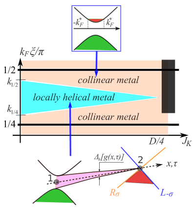
Figure 1: Central Panel: Phase diagram of the magnetically doped 1D quantum wire for $J_{K}\ll E_{F}$, see explanations in the text; here $|k_{f}-f\pi/\xi|\sim J_{K}/v_{F},\ f=1/4,1/2$. Upper panel: band structure of the non-helical collinear metal with the renormalized Fermi-momentum, $k_{F}^{*}$. Green and red areas denote filled valence- and partially occupied conduction- bands, respectively. Lower panel: band structure and local helicity of the novel metallic phase. At some space-time point “1”, the local spin ordering can open a gap, $\Delta_{h}$, in the spectrum of the fermions $\{R_{\sigma},L_{-\sigma}\}$ with a given helicity, $h$. The second helical sector, $\{R_{-\sigma},L_{\sigma}\}$ (not shown on this illustration for simplicity), remains gapless at the point “1”. The gap of the fermions $\{R,L\}$ slowly varies in space-time due to spin fluctuations described by the SU(2) matrix $g$. There can exist another space-time point “2” where $\Delta_{h}\to 0$, $|\Delta_{-h}|\to{\rm max}$ and, thus, the gapped (gapless) helical sector becomes gapless (gapped). Hence, the global helicity cannot be defined though transport remains protected as in the case of the globally helical quantum wires.

Thus, further progress in obtaining the helical quantum wires, in particular by means of the magnetic doping, has been hampered by two open questions: (i) Is the global helicity accompanied by breaking the spin-rotation symmetry really necessary to obtain HM? (ii) If the global helicity is not really needed, which parameters must be tuned for detecting HM in the KLs (theoretically) and in the magnetically doped quantum wires (experimentally)? We note that numerical studies have never provided a reliable signature of the helical phase in the KLs McCulloch et al. (2002); Smerat et al. (2011); Khait et al. (2018).

In this Paper, we answer both questions: Protection of the ballistic transport can be provided by the local helicity which, paradoxically, requires neither the global helicity nor breaking the spin-rotation symmetry. We show that such a novel HM is the $4k_{F}$ charge-density-wave (CDW) phase Giamarchi (2004) where all effects of disorder are parametrically suppressed. It can be found in the isotropic KLs if the Kondo exchange coupling is much smaller than the Fermi energy and the band width, $J_{K}\ll E_{F},D$, and the band filling is far from special commensurate cases (1/4-, 3/4-, 1/2-fillings), see Fig.1. To the best of our knowledge, this is the first prediction of the helicity-protected transport in the quantum 1D system where the spin-rotation symmetry exists and cannot be spontaneously broken. Our results pave the way towards novel numerical and experimental investigations of the HM.

II Theoretical model

We start from the standard KL Hamiltonian:

$$\hat{H}=-\!\sum_{n}\Big{[}t\,\psi^{\dagger}_{n}\psi_{n+1}+h.c.+\mu\,\rho_{n}-J_{K}\psi_{n}^{+}{\bm{\sigma}}{\bm{S}}_{n}\psi_{n}\Big{]}.$$ (1)

Here $\psi_{n}\equiv\{\psi_{n,\uparrow},\psi_{n,\downarrow}\}^{\rm T}$  are electron annihilation ($\psi^{\dagger}_{n}$ - creation) operators; $\rho_{n}=\psi^{\dagger}_{n}\psi_{n}$; ${{\bm{S}}}_{n}$ are quantum spins with magnitude $s$; ${\bm{\sigma}}\equiv\{\sigma_{x},\sigma_{y},\sigma_{z}\}$ are Pauli matrices; $t$ and $\mu$ are the electron hopping and the chemical potential; summation runs over lattice sites. We assume that $sJ_{K}<D=2t$ and consider low temperatures, $T\to 0$.

III Method

We proceed in several steps. Firstly, we find classical spin configurations minimizing the free energy. Secondly, we identify degrees of freedom whose fluctuations are gapped, including gapped fermionic and spin variables ($|{\bf m}|$ and $\alpha$ in Eq.(III.1) below) and integrate out the gapped variables perturbatively. Remaining spin fluctuations [described by vectors ${\bm{e}}_{a}$ in Eq.(III.1)] receive the fully quantum mechanical treatment. This approach is justified by the separation of scales: the shortest scale is of order of the inverse Fermi momentum, $1/k_{F}$. It is present in the spin ordering and must be much smaller then the coherence length $\zeta$ of the gapped variables. We have performed the self-consistency check which confirms that $\zeta\gg 1/k_{F}$ and, thus, justifies the validity of our theory.

III.1 Separating the slow and the fast variables

To describe an effective low energy theory, it is convenient to focus on the regime $|J_{K}|<|\mu|\ll t$ where we can linearize the dispersion relation and introduce right-/left moving fermions, $\psi_{\pm}$, in the standard way Giamarchi (2004). In the continuum limit, the fermionic Lagrangian reads

$${\cal L}_{F}[\psi_{\pm}]=\sum_{\nu=\pm}\psi^{\dagger}_{\nu}\partial_{\nu}\psi_{\nu}\,;\quad\partial_{\pm}\equiv\partial_{\tau}\mp iv_{F}\partial_{x}\,.$$ (2)

Here $v_{F}$ is the Fermi velocity, $\nu$ is the chiral index which indicates the direction of motion, $\partial_{\nu}$ is the chiral derivative, $\tau$ is the imaginary time.

According to Doniach’s criterion, the RKKY interaction wins in 1D when the distance between the spins is smaller then a crossover scale: $\,\xi_{s}<\xi\sqrt{\vartheta_{0}J_{K}^{2}/T_{K}}\,$; here $\,\xi\,$ is the lattice spacing, $\vartheta_{0}$ is the density of states at $E_{F}$; $T_{K}$ is the Kondo temperature. We study this RKKY-dominated regime. For simplicity, we assume $\xi_{s}=\xi$.

Following Refs.Tsvelik (1994); Tsvelik and Yevtushenko (2015); Schimmel et al. (2016), we keep in the Lagrangian of the electron-KI interaction only the backscattering terms governing the physics of the dense 1D KL:

$${\cal L}_{\rm bs}(n)=J_{K}\left[R^{\dagger}_{n}{\bm{\sigma}}{\bm{S}}_{n}L_{n}e^{-2ik_{F}x_{n}}+h.c\right],\ x_{n}\equiv n\xi\,;$$ (3)

where $R\equiv\psi_{+},\,L\equiv\psi_{-}$. ${\cal L}_{\rm bs}$ contains the fast $2k_{F}$-oscillations which must be absorbed into the spin configuration. We perform this step using the path integral approach where the spin operators are replaced by integration over a normalized vector field decomposed as

$${\bm{S}}_{n}/s={\bm{m}}+b\Big{(} {\bm{e}}_{1} \,\cos(\alpha)\cos(qx_{n}+\theta)+$$

$${\bm{e}}_{2} \,\sin(\alpha)\sin(qx_{n}+\theta)\Bigr{)}\sqrt{1-{\bm{m}}^{2}}\,.$$

Here $q\simeq 2k_{F}$; $\{{\bm{e}}_{1},{\bm{e}}_{2},{\bm{m}}\}$ is an orthogonal triad of vector fields whose coordinate dependence is smooth on the scale $1/k_{F}$, $|{\bm{e}}_{1,2}|=1$. Angle $\alpha$ and constants $b,\theta$ must be chosen to maintain normalization $|{\bm{S}}/s|=1$. Eq.(III.1) is generic; it allows for only three possible choices of the constants which, in turn, reflect the band filling $f$, see Suppl.Mat. A. After inserting Eq.(III.1) into Eq.(3), we select the non-oscillatory parts of ${\cal L}_{\rm bs}$ for these three cases, and take the continuous limit. This yields the smooth part of the Lagrangian density:

• $f=1/2,\,2k_{F}x_{n}=\pi n$:

  $$b=1,\ \theta=\alpha=0,\ {\cal L}_{\rm bs}^{(1/2)}=\tilde{J}\left(\tilde{R}^{\dagger}\sigma_{x}\tilde{L}+h.c\right);$$ (5)

• $f=1/4,\,2k_{F}x_{n}=\pi n/2$:

  $$b = \sqrt{2},\ \theta=\pi/4,\ \alpha\in[0,2\pi];$$ (6)

  $${\cal L}_{\rm bs}^{(1/4)} = \frac{\tilde{J}}{\sqrt{2}}\left(e^{i\pi/4}\tilde{R}^{\dagger}[\cos(\alpha)\sigma_{x}+i\sin(\alpha)\sigma_{y}]\tilde{L}+h.c\right);$$

• generic filling:

  $$b=\sqrt{2},\theta=0,\alpha=\pi/4;\,{\cal L}_{\rm bs}^{\rm(gen)}=\tilde{J}\left(\tilde{R}^{\dagger}\sigma_{-}\tilde{L}+h.c\right)\!\!.$$ (7)

Here $\tilde{J}\equiv sJ_{K}\sqrt{1-{\bm{m}}^{2}}/2$; $\sigma_{\pm}=(\sigma_{1}\pm i\sigma_{2})/2$; we expressed vectors ${\bm{e}}_{1,2}$ via matrix $g\in\mbox{SU(2)}$, see Suppl.Mat. B. $g$ is a smooth function of $\{x,\tau\}$; it governs the new rotated fermionic basis

$$\tilde{R} \equiv g^{-1}R,\ \tilde{L}\equiv g^{-1}L\,;$$ (8)

$${\cal L}_{F}[\tilde{R},\tilde{L}] = \tilde{R}^{\dagger}(\partial_{+}+g^{-1}\partial_{+}g)\tilde{R}+\tilde{L}^{\dagger}(\partial_{-}+g^{-1}\partial_{-}g)\tilde{L}.$$

Eq.(5) assumes a staggered configuration of spins at half-filling, $\uparrow\downarrow$, which was studied in Ref.Tsvelik (1994). The spin sector of the half-filled KL is an antiferromagnet where the spins fluctuate around the Neel order with a finite correlation length. Eq.(6) reflects two spins up- two spins down configuration, $\uparrow\uparrow\downarrow\downarrow$, which agrees with the spin dimerization tendency observed numerically in Ref.Xavier et al. (2003) at quarter-filling. Eq.(7) is a rotationally invariant counterpart of the helical spin configuration discovered in Refs.Tsvelik and Yevtushenko (2015); Schimmel et al. (2016) in the anisotropic KL at incommensurate fillings. Spins fluctuate around this configuration. Detailed derivation of their effective action is presented in Ref.Tsvelik and Yevtushenko (2019). A simplified version of Eq.(7) was used in Ref.Fazekas and Müller-Hartmann (1991) for analyzing magnetic properties of KLs. Below, we refer to Eqs.(5,6) at $\alpha=0$ as “commensurate configurations” and to Eqs.(6,7) at $\alpha=\pi/4$ as “general configurations”. We note that the low energy physics of KLs with the 1/4- and 3/4-filling is equivalent in our model. Therefore, we will discuss only 1/4-filling and do not repeat the same discussion for the case of the 3/4-filling.

IV Results

Let us start from the presentation of our results at the simplified and transparent semiclassical level.

IV.1 Fermionic gap

The backscattering described by Eqs.(5-7) opens a gap in the spectrum of the rotated fermions $\tilde{R},\tilde{L}$. It decreases their ground state energy: the larger the gap, the greater is the gain in the fermionic kinetic energy. Since the spin degrees of freedom do not have kinetic energy, the minimum of the ground state energy is achieved by maximizing the fermionic gap. This indicates that $|{\bm{m}}|$ is the gapped variable with the classical value $m_{0}=0$. Below, we use $m_{0}$ for the semiclassical part of the discussion.

The KL contains two fermionic sectors which can have different gaps depending on the band filling and the spin configuration. The gaps can be found from Eqs.(5-7):

$$f=1/2: \Delta^{(1/2)}_{1,2}=\tilde{J};$$ (9)

$$f=1/4: \Delta^{(1/4)}_{1,2}=\tilde{J}(\cos(\alpha)\pm\sin(\alpha))/\sqrt{2};$$ (10)

$$\mbox{generic filling}: \Delta^{\rm(gen)}_{1}=\tilde{J},\ \Delta^{\rm(gen)}_{2}=0.$$ (11)

The gain in the fermionic ground state energy reads

$$\delta E_{\rm GS}=-\vartheta_{0}\,\xi\sum_{k=1,2}\Delta^{2}_{k}\log\bigl{(}D/|\Delta_{k}|);$$ (12)

see Suppl.Mat. C. $\vartheta_{0}=1/\pi v_{F}$ for the 1D Dirac fermions. Let us now analyze various band fillings.

IV.2 Special commensurate fillings, insulating KLs

At $f=1/2,1/4$, we have to decide which spin configurations - the commensurate ones [Eq.(5) for $f=1/2$ and Eq.(6) with $\alpha=0,\pi/2$ for $f=1/4$] or the generic configuration - minimize the ground state energy. Using Eqs.(9-12), we obtain

$$\delta E_{\rm GS}(\Delta^{(1/2)})\!-\!\delta E_{\rm GS}(\Delta^{\rm(gen)})=-{\cal E}\log\left(D/|\tilde{J}|\right)\!,$$ (13)

$$\delta E_{\rm GS}\left(\Delta|^{(1/4)}_{\alpha=0}\right)\!-\!\delta E_{\rm GS}\left(\Delta|^{(1/4)}_{\alpha=\pi/4}\right)=\!-\!{\cal E}\log(\sqrt{2});$$ (14)

with $\,{\cal E}\equiv\vartheta_{0}\xi\tilde{J}^{2}\,$. In both commensurate cases, the commensurate configuration wins, the conduction band of such KLs is empty and, hence, they are insulators, as expected. Note that, at quarter-filling, the minimum of $\delta E_{\rm GS}$ is provided by $\alpha=0$ which means that $\alpha$ is gapped.

IV.3 Vicinity of special commensurate fillings, collinear metal and heavy TLL

Let us consider fillings which are slightly shifted from the special commensurate cases. To be definite, we analyze an upward shift; a downward shift can be studied in much the same way. Eqs.(13-14) suggest that the commensurate spin configuration remain energetically favorable even close to the commensurate filling. The wave vector $q$ of the spin modes remains commensurate, Eqs.(5,6), and is slightly shifted from $2k_{F}$: $2k_{F}-q\equiv Q\ll 1/\xi$ with $q=2\pi f/\xi$ and $f=1/2,1/4$. This case is described in terms of Dirac fermions with a non-zero chemical potential:

$$\bar{{\cal L}}={\cal L}_{F}[R,L]+{\cal L}_{\rm bs}^{(f)}[R,L]-(v_{F}Q/2)(R^{\dagger}R+L^{\dagger}L),$$ (15)

see Suppl.Mat. D. Backscattering by the commensurate spin configuration opens a gap below the chemical potential. The electrons with energies $0<E\leq v_{F}Q/2$ are pushed above the gap, Fig.1, and have (almost) parabolic dispersion:

$$E^{+}(k)\bigl{|}_{v_{F}|k|<|\tilde{J}|}\simeq|\tilde{J}|+\left(v_{F}k\right)^{2}/2|\tilde{J}|\,;$$ (16)

see Eq.(D4). Since this new phase possesses a partially filled band it is a metal. Its metallic behavior originates from the (almost) collinear spin configuration whose classic component is governed by only one slowly rotating vector, e.g. ${\bm{e}}_{1}$. We will reflect this fact by referring to such phases as “collinear metals” (CMs).

A detail description of CMs is presented in Ref.Tsvelik and Yevtushenko (2019). Let us mention here that spin modes can mediate repulsion between the conduction electrons and, for energies $|E-E^{+}(k_{F}^{*})|\ll E^{+}(k_{F}^{*})$, they form a repulsive and spinful TLL characterized by a new Fermi momentum $k^{*}_{F}=Q/2$. If the effective repulsion is strong enough, TLL becomes heavy. Such TLL has been observed numerically in Ref.Khait et al. (2018). 1D nature makes repulsive CMs very sensitive to spinless impurities: even a weak disorder easily drives it to the localized regime with suppressed dc transport Giamarchi and Schulz (1988).

IV.4 Quantum phase transition at generic filling

The CM becomes less favorable when $|Q|$ increases: the energy of the electrons in the TLL, $E_{\rm p}\simeq\xi\tilde{J}k_{F}^{*}/\pi+\xi v_{F}^{2}(k_{F}^{*})^{3}/6\pi\tilde{J}$, becomes large when $k_{F}^{*}=Q/2$ increases, Fig.1. If $|Q|$ is large enough, such that $\,E_{\rm p}\geq{\cal E}\,$, the minimum of the ground state energy is provided by the generic spin configuration, Eq.(7). Equalizing the leading part of $E_{\rm p}$ with ${\cal E}$, we can estimate the critical value of $Q$ at which the spin configuration changes: $Q_{c}\sim\tilde{J}/v_{F}$. If $\tilde{J}\ll v_{F}/\xi\sim D$, there is always a parametrically large window of the band fillings where the new phase is realized, see Fig.1. If $\tilde{J}\to D/4$, this window shrinks to zero and the CM dominates at all fillings excluding special commensurate cases 1/2, 1/4; see Fig.1. The spin configuration cannot change gradually. The switching from the commensurate to the generic configuration is always abrupt and, therefore, $Q_{c}$ is the point of a quantum phase transition.

IV.5 Generic incommensurate fillings,
locally helical metal

The remaining case of generic filling, Eq.(7), is the most promising for transport because rotated fermions are gapped only in one helical sector, e.g. $\{\tilde{R}_{\downarrow},\tilde{L}_{\uparrow}\}$, and the second helical sector, $\{\tilde{R}_{\uparrow},\tilde{L}_{\downarrow}\}$, remains gapless, see Eq.(11) and Fig.1. The semiclassically broken helical symmetry is restored by the fluctuations: The rotating matrix field $g(x,\tau)$ slowly changes in space and time around the underlying spin spiral and, therefore, the global helicity cannot appear, see Fig.1. Hence, one can describe properties of the new phase only in terms of the local helicity. Simultaneously, there are no sectors of the physical fermions, $\{R_{\sigma},L_{\sigma}\}$, which can be found from the inverse of the rotation Eq.(8), which are either gapless or globally helical. To emphasize the underlying locally helical spin configuration, we refer to this phase as “locally-helical metal” (lHM).

Since neither the spins nor the physical charge carriers in the lHM possess the global helicity, one can surmise that they are not a platform for a protected transport. This is, however, incorrect since the most significant property of the lHMs is that they inherit protection of the ballistic transport from those HMs where SU(2) symmetry is broken and the global helicity emerges Tsvelik and Yevtushenko (2015); Schimmel et al. (2016). The absence of the global helicity in lMHs is reflected in the gapped nature of the spin excitations Tsvelik and Yevtushenko (2019)

IV.6 Origin of protection

Let us explain the physics of the seemingly counterintuitive protected transport in the lHMs. The density and backscattering operators are invariant under $g$-rotation: $R^{\dagger}R=\tilde{R}^{\dagger}\tilde{R},\,L^{\dagger}L=\tilde{L}^{\dagger}\tilde{L},\,R^{\dagger}L=\tilde{R}^{\dagger}\tilde{L}$. The low energy physics is governed by fields whose correlation functions decay as power law. To obtain them, we project the fields on the gapless sector, i.e., average over the high energy gapped modes. For example, components of the charge density are:

$$\rho(0) = \tilde{R}^{\dagger}_{\uparrow}\tilde{R}_{\uparrow}+\tilde{L}^{\dagger}_{\downarrow}\tilde{L}_{\downarrow}\,;$$ (17)

$$\rho(4k_{F}) \sim e^{-4ik_{F}x}\tilde{R}^{\dagger}_{\uparrow}\langle\tilde{R}^{\dagger}_{\downarrow}\tilde{L}_{\uparrow}\rangle\tilde{L}_{\downarrow}+h.c.$$

$\rho(2k_{F})$ is absent because it would correspond to a single particle elastic backscattering between the gapless and gapped fermions which is not allowed. This is the direct consequence of the (local) spin helix which gaps out only one helical fermionic sector. Thus, the HM is the $4k_{F}$-CDW phase. This fact has two important consequences: (i) the (local) spin helix shifts the Friedel oscillations of the charge density from $\,2k_{F}\,$ to $\,4k_{F}\,$, which is indistinguishable from $\,4(k_{F}-\pi/2\xi)\,$ due to the lattice periodicity; (ii) even more importantly, it drastically reduces backscattering caused by spinless disorder.

To illustrate the 2nd statement, we introduce a random potential of spinless backscattering impurities which couples to the $2k_{F}$-component of density ${\cal L}_{\rm dis}=V_{2k_{F}}\,\tilde{R}^{\dagger}\tilde{L}+h.c.$ Here $V_{2k_{F}}$ is a smooth $2k_{F}$-component of the random potential. Since the charge response function of lHM at the $2k_{F}$ wave-vector is non-singular, backscattering can occur only via many particle processes with much smaller amplitude. Averaging over the gapped fermions, we find: $\langle{\cal L}_{\rm dis}\rangle\simeq 2\left(V_{2k_{F}}^{2}/\Delta^{\rm(gen)}\right)\,\tilde{R}^{\dagger}_{\uparrow}\tilde{L}_{\downarrow}+h.c.$ see Suppl.Mat. E. If the helical gap is large enough, $\Delta^{\rm(gen)}=\tilde{J}\gg V_{2k_{F}}$, backscattering and all disorder effects are parametrically suppressed.

V Quantum theory for smooth spin variables and self-consistency check

To complete the theory of the magnetically doped quantum wires, one must consider quantum fluctuations of smooth spin variables ${\bm{e}}_{1,2}$. They are described by using the heavy field-theoretical machinery of the nonlinear $\sigma$-model (nLSM). Its derivation is a lengthy task which is described in detail in Ref.Tsvelik and Yevtushenko (2019). Here, we very briefly recapitulate main steps of the derivation, give final answers, and argue that the fully quantum mechanical theory does not violate separation of scales, see Sect.III. The latter is especially important since it confirms validity of our approach and validates results described in the previous Section at the simplified and transparent semiclassical level.

Derivation of the nLSM requires several steps:

• One (i) integrates out gapped fermions and exponentiates the fermionic determinant; (ii) derives the Jacobian of the SU(2) rotation by the matrix $g$; (iii) selects smooth contributions from the Wess-Zumino term for the spin field Tsvelik (2003). The commensurate spin configurations generate also the topological term (see Ref.Tsvelik (1994), Sect.16 of the book Tsvelik (2003), and references therein).

• The total Lagrangian, which is obtained by summing up the exponentiated fermionic determinant, the Jacobian, the Wess-Zumino contributions and the topological terms, is expanded in gradients of the matrix $g$ and in small fluctuations of $|{\bm{m}}|$ around its classical value $m_{0}=0$. The commensurate spin configuration, which corresponds to 1/4-filling, requires also the expansion in fluctuations of $\alpha$.

• Finally, fluctuations of $|{\bm{m}}|$ (and of $\alpha$, if needed) are integrated out in the Gaussian approximation.

These steps result in the quantum mechanical nLSM in (1+1) space-time dimensions which describes the smooth spin degrees of freedom. Our approach is self-consistent if typical scales of the quantum theory remain large, $\geq v_{F}/\tilde{J}\gg k_{F}^{-1}$. The nLSM is different in different phases.

Commensurate insulators and collinear metals: The action of the nLSM describing fluctuations of the spin variables in a commensurate insulator and in a collinear metal takes the following form:

$$S^{(f)} = \int{\rm d}\tau{\rm d}x{\cal L}^{(f)}+S_{\rm top},\,S_{\rm top}=(2s-1)i\pi k\,;$$ (18)

$${\cal L}^{(f)} = \frac{1}{2g_{f}}\left[\frac{(\partial_{\tau}{\bm{e}}_{1})^{2}}{c_{f}}+c_{f}(\partial_{x}{\bm{e}}_{1})^{2}\right].$$

Here $f=1/2$ at (or close to) the half-filling and $f=1/4$ at (or close to) the quarter-filling; small dimensionless coupling constants, $g_{1/2}\simeq(4\pi/s)\,\vartheta_{0}\xi\tilde{J}\sqrt{\log\Bigl{(}D/|\tilde{J}|\Bigr{)}}\ll 1$ and $g_{1/4}\simeq g_{1/2}/\sqrt{8}\ll 1$, determine small renormalized velocities of the spin excitations, $c_{f}=v_{F}g_{f}/4\pi\ll v_{F}$. Smallness of $g_{f}$ and $c_{f}$ reflects the coupling between spins and gapped (localized) fermions. The integer $k$ marks topologically different sectors of the theory.

The action $S^{(f)}$ corresponds to the well-known O(3)-symmetric nLSM in (1+1) dimensions with the topological term. It is exactly solvable Wiegmann (1985); Fateev and Zamolodchikov (1991); Tsvelik (2003) and possesses a characteristic energy ${\cal E}_{f}\sim|\tilde{J}|g_{f}^{-1}\exp(-2\pi/g_{f})$ which governs a large spatial scale: $c_{f}/{\cal E}_{f}\gg v_{F}/\tilde{J}\gg k_{F}^{-1}$. The latter inequality confirms validity of our approach.

Locally-Helical metals: The Largangian of the nLSM describing fluctuations of the spin variables in a lHM takes the following form:

$${\cal L}^{\rm(hel)}=\frac{1}{2g_{\rm hel}}\left\{\frac{\left[\Omega_{\tau}^{(z)}\right]^{2}}{c_{\rm hel}}+c_{\rm hel}{\rm tr}(\partial_{x}g^{+}\partial_{x}g)\right\}\,;$$ (19)

with $g_{\rm gen}\simeq g_{1/4}/4\ll 1$, $c_{\rm gen}=v_{F}g_{\rm gen}/\pi\ll v_{F}$, and $\Omega_{\tau}^{(z)}\equiv i{\rm tr}[\sigma_{z}g^{-1}\partial_{\tau}g]/2$. This theory is anisotropic and has the SU(2)-symmetry, $g\to{\cal M}g,\,{\cal M}\in\mbox{ SU(2)}$. The time derivative is present only in the $\Omega^{z}$ term. This points to a relatively short bare correlation length of spins which coincides with the UV cut-off of the theory. The latter is $\sim v_{F}/\tilde{J}$ in our approach and does not violate the self-consistency requirement because $v_{F}/\tilde{J}\gg\xi$. The actual shortest scale of the theory is expected to be much larger if the anisotropy is irrelevant and ${\cal L}^{\rm(gen)}$ flows in the IR limit to the well-known SU(2)$\times$SU(2)-symmetric nLSM. An example of such a behaviour is provided by the RG equations derived in Ref.Azaria et al. (1992) for the (2+1) dimensions. There is no counterargument against the irrelevance of the anisotropy in the (1+1) dimensions. Therefore, we arrive at a conclusion that the shortest spatial scale generated by ${\cal L}^{\rm(hel)}$ is $\gg v_{F}/\tilde{J}\gg k_{F}^{-1}$.

This concludes the self-consistency check of our approach and justifies qualitative results described in Sect.IV at the semiclassical level.

VI Possible numerical and experimental test of our theory

An important task for the subsequent research is to reliably detect different metallic phases in the 1D KLs (numerically) and in the magnetically doped quantum wires (experimentally). This requires to tune the band filling and the Kondo coupling. The key features distinguishing CM and lHM in numerics and experiments are as follows. The conductance of the CM is equal to the quantum $G_{0}=2e^{2}/h$ while the lHM must show only $G_{0}/2$ conductance due to the helical gap. The CM is a spinful TLL whose charge and spin response functions have a peak at $2k_{F}^{*}$; $k_{F}^{*}$ is the shifted Fermi momentum predicted by general theorems Yamanaka et al. (1997); Oshikawa (2000). The lHM is the $4k_{F}$-CDW and has singular response in the charge sector. Since $4k_{F}$ and $4k_{F}^{*}$ are indistinguishable on the lattice the response of the lHM does not show the shift $k_{F}\to k_{F}^{*}$. Unlike systems with broken SU(2) symmetry Tsvelik and Yevtushenko (2015); Schimmel et al. (2016), the lHM, which we have considered, does not have singular response in the spin sector. Inasmuch as the CM responds to scalar potentials at $2k_{F}^{*}$ and the lHM - at $4k_{F}$, the spinless disorder potential has a profound difference with respect to transport in the CM and lHM phases. Namely, localization is parametrically suppressed in the lHM.

Detecting the CM is not difficult because it is generic at relatively large $J_{K}$ and filling away from 1/2, 1/4. The heavy TLL, which is formed by the interactions in the CM, has been observed in numerical results of Ref.Khait et al. (2018). However, $J_{K}$ was too large for finding the HM. The KL studied in Ref.Smerat et al. (2011) exhibits an unexpected $2k_{F}$-peak at small $J_{K}$. Yet, the peak was detected in the spin susceptibility of 6 fermions distributed over 48 sites. So small KL cannot yield a conclusive support or disproof of our theory. A more comprehensive study of the larger KLs is definitely needed.

The thorough control of the system parameters is provided by the experimental laboratory of cold atoms where 1D KL was recently realized Riegger et al. (2018). Experiments in cold atoms are, probably, the best opportunity to test our theory. However, modern solid-state technology also allows one to engineer specific 1D KL even in solid state platforms. It looks feasible to fabricate 1D KL in clean 1D quantum wires made, e.g., in GaAs/AlGaAs by using cleaved edge overgrowth technique Pfeiffer et al. (1993) or in SiGe Mizokuchi et al. (2018). Magnetic adatoms can be deposited close to the quantum wire by using the precise ion beam irradiation. One can tune parameters of these artificial KLs by changing the gate voltage, type and density of the magnetic adatoms and their proximity to the quantum wire. Such a nano-engineering of 1D KL is essentially similar to the successful realization of topological superconductivity in atomic chains Feldman et al. (2017), in carbon nanotubes Desjardins et al. (2019), and in Bi Jäck et al. (2019). The experiments should be conducted at low temperatures, $T\ll\Delta,{\cal E}$, where destructive thermal fluctuations are weak.

VII Conclusions

We have studied the physics of quantum wires functionalized by magnetic adatoms with a high density and a small coupling between the itinerant electrons and local magnetic moments of the ad-atoms, $|J_{K}|\ll E_{F}$. Their physics is determined by the RKKY interaction between the ad-atoms which results in a quite rich phase diagram. It includes: (i) the insulating phase which appears at special commensurate band filling, either 1/2, or 1/4, 3/4; (ii) spinful interacting metals which exist in the vicinity of that commensurate fillings; and (iii) the novel metallic phase at generic band fillings, see Fig.1.

The third phase is our most important and intriguing finding. On one hand, the local spins form a slow varying in space and time spiral, which can yield a local helical gap of the electrons. On the other hand, the global helicity is absent because the spin-rotation symmetry is not (and cannot) be broken. The latter can result in an erroneous conclusion that a helicity-protected transport could not originate in these locally helical metals. That is not true: paradoxically, the locally helical phase inherits protection of the ballistic transport from those systems where the spin rotation symmetry is broken and the global helicity emerges. Protection of transport in lHMs has a simple physical explanation because they are the $4k_{F}$-CDW phase with the reduced $2k_{F}$ response. This reduction is the direct consequence of the local helicity. It parametrically suppresses effects of a spinless disorder and localization. Thus, we come across the principally new type of emergent (partial) protection of transport caused by the interactions without a need of the global helicity. Our model and approach allow us to uncover the promising possibility for engineering the HM in the quantum wires and to identify the parameter range where the HM is formed, see Fig.1. To the best of our knowledge, this gives the firstever example of such a protection in the system where the spin-rotation symmetry is not (and cannot be) broken. It would be interesting to study in the future how the direct Heisenberg interaction between the spins could modify out theory Tsvelik and Yevtushenko (2017); Yevtushenko and Tsvelik (2018).

We believe that detecting the lHMs in numerical simulations and real experiments is the task of a high importance. Our results suggest how to tune the physical parameters, in particular the band filling and the Kondo coupling, such that the lHM could be realized. The fundamental sensitivity of the state and of the transport properties of the magnetically doped quantum wire to the band filling is especially important. It allows one to switch over normal and locally helical regimes of the conductor by varying a gate voltage. This can be used for creating fully controllable helical elements. Our theoretical prediction, that the backscattering is suppressed in the lHMs in spite of the absence of the global helicity, can pave the way towards flexible engineering principally new units of nano-electronics and spintronics with substantially improved efficiency.

Suppl.Mat. A Decomposition of a normalized vector field into constant and oscillating parts

Let us consider a unit-vector field, ${\bm{s}}$ with $|{\bm{s}}|=1$, and single out its zero mode and $\pm q$ components:

$${\bm{s}}={\bm{s}}_{0}+{\bm{s}}_{c}\cos(qx+\theta)+{\bm{s}}_{s}\sin(qx+\theta)\,.$$ (20)

Here $\theta$ is a constant phase shift; coefficients ${\bm{s}}_{0,c,s}$ must be smooth functions on the scale of $1/q$. The normalization of ${\bm{s}}$ must hold true for arbitrary $x$. This always requires mutual orthogonality

$$({\bm{s}}_{0},{\bm{s}}_{c})=({\bm{s}}_{0},{\bm{s}}_{s})=({\bm{s}}_{c},{\bm{s}}_{s})=0\,;$$ (21)

and proper normalizations:

$$\mbox{generic $q$}: |{\bm{s}}_{c}|=|{\bm{s}}_{s}|,\ |{\bm{s}}_{0}|^{2}+|{\bm{s}}_{c}|^{2}=1\,;$$ (22)

$$\sin(qx+\theta)=0: |{\bm{s}}_{0}|^{2}+|{\bm{s}}_{c}|^{2}=1\,,\qquad\mbox{ or }\quad\cos(qx+\theta)=0:\qquad|{\bm{s}}_{0}|^{2}+|{\bm{s}}_{s}|^{2}=1\,;$$ (23)

$$e^{i(qx+\theta)}=\pm\frac{1\pm i}{\sqrt{2}}: |{\bm{s}}_{0}|^{2}+\frac{|{\bm{s}}_{c}|^{2}+|{\bm{s}}_{s}|^{2}}{2}=1\,.$$ (24)

There are no other configurations which are compatible with decomposition Eq.(20).

Suppl.Mat. B Useful relations

Using the matrix identities

$$\left\{\begin{array}[]{l}\hat{A}=A^{(j)}\sigma_{j},\quad A^{(j)}=\frac{1}{2}{\rm tr}[\sigma_{j}\hat{A}];\\ \\ {\rm tr}[{\bm{\sigma}}\hat{A}^{-1}\sigma_{j}\hat{A}]\,{\rm tr}[{\bm{\sigma}}\hat{A}^{-1}\sigma_{j^{\prime}}\hat{A}]=4\delta_{j,j^{\prime}}\end{array}\right.\qquad j,j^{\prime}=x,y,z.$$ (25)

and re-parameterizing the (real) orthogonal basis ${\bm{e}}_{1,2,3}$ in terms of a matrix $g\in\mbox{SU(2)}$:

$${\bm{e}}_{1,2,3}=\frac{1}{2}{\rm tr}[{\bm{\sigma}}g\sigma_{x,y,z}g^{-1}]\,,\quad{\bm{e}}_{3}=[{\bm{e}}_{1}\times{\bm{e}}_{2}]\,,\quad\sum_{a=1,2,3}(\partial_{\alpha}{\bm{e}}_{a})^{2}=4{\rm tr}[\partial_{\alpha}g^{-1}\partial_{\alpha}g]\,;$$ (26)

we can re-write a scalar product $({\bm{\sigma}},e_{j})$ as follows:

$$({\bm{\sigma}},{\bm{e}}_{1,2})=\frac{1}{2}g\sigma_{x,y}g^{-1}\quad\Rightarrow\quad({\bm{\sigma}},[{\bm{e}}_{1}\pm i{\bm{e}}_{1}])=g\sigma_{\pm}g^{-1}\,;\quad\sigma_{\pm}\equiv(\sigma_{x}\pm i\sigma_{y})/2.$$ (27)

One can also do an inverse step and express the SU(2) matrix via a unit vector

$$g=i({\bm{\sigma}},{\bm{n}}),\ g^{-1}=-i({\bm{\sigma}},{\bm{n}})\,;\ |{\bm{n}}|=1\,\quad\Rightarrow\quad g^{-1}\partial_{\alpha}g=i\bigr{(}{\bm{\sigma}},[{\bm{n}}\times\partial_{\alpha}{\bm{n}}]\bigl{)}\,.$$ (28)

Suppl.Mat. C Ground state energy of the gapped 1D Dirac fermions

Consider 1D Dirac fermions with the inverse Green’s function:

$$[\hat{G}(\Delta)]^{-1}=\left(\begin{array}[]{cc}\partial_{+}&\Delta\\ \Delta&\partial_{-}\end{array}\right)\,\underrightarrow{\rm FT}\,\left(\begin{array}[]{cc}-i\omega_{n}+v_{F}k&\Delta\\ \Delta&-i\omega_{n}-v_{F}k\end{array}\right).$$ (29)

Integrating out the fermions we find the partition function:

$$Z[\Delta]=Z_{0}\frac{\det\left([\hat{G}(\Delta)]^{-1}\right)}{\det\left([\hat{G}_{0}]^{-1}\right)}=Z_{0}\exp\left(-{\rm Tr}\left(\log\left[\hat{G}_{0}^{-1}\hat{G}(\Delta)\right]\right)\right)\simeq Z_{0}\exp\left(-{\rm Tr}\left[\hat{G}_{0}^{-1}\hat{G}(\Delta)-1\right]\right)\,.$$ (30)

Here $Z_{0}\equiv Z[\Delta=0]$, $\hat{G}_{0}\equiv\hat{G}[\Delta=0]$ and $\Delta$ is assumed to be small. Using the expression for the free energy ${\cal F}=-T\log[Z]$, we find that the gain of the energy, which is caused by the gap opening, reads as

$$\delta E_{\rm GS}=T\,{\rm Tr}\left[\hat{G}_{0}^{-1}\hat{G}(\Delta)-1\right]$$ (31)

At $T=0$ and in the continuous limit, this expression reduces to

$$\delta E_{\rm GS}=-2\xi\int\frac{{\rm d}^{2}\{\omega,q\}}{(2\pi)^{2}}\frac{\Delta^{2}}{\omega^{2}+(v_{F}q)^{2}+\Delta^{2}}\,.$$ (32)

The UV divergence must be cut by the band width $D$. Thus, we obtain with the logarithmic accuracy:

$$\delta E_{\rm GS}\simeq-\frac{\xi}{\pi v_{F}}\Delta^{2}\log\bigl{(}D/|\Delta|)\,.$$ (33)

Suppl.Mat. D Smoothly oscillating backscattering

The theory close to the special commensurate filling can be formulated in terms of Dirac fermions with a spatially oscillating backscattering described by Lagrangian:

$${\cal L}_{\rm osc}=\left(\begin{array}[]{cc}\partial_{+}&Je^{-iQx}\\ Je^{iQx}&\partial_{-}\end{array}\right).$$ (34)

The wave vector $Q$ is a deviation of $2k_{F}$ from its special commensurate value. By rotating the fermions

$$R\to e^{-iQx/2}R,\ L\to e^{iQx/2}L,$$ (35)

we reduce ${\cal L}_{\rm osc}$ to the Lagrangian with the constant backscattering and with the shifted chemical potential:

$$\bar{{\cal L}}_{\rm osc}=\left(\begin{array}[]{cc}-i\omega_{n}+v_{F}k&J\\ J&-i\omega_{n}-v_{F}k\end{array}\right)-\frac{v_{F}Q}{2}.$$ (36)

Backscattering opens the gap in the fermionic spectrum but at the energy level shifted from zero by $v_{F}Q/2$. Thus, the dispersion relation counted from the shifted chemical potential reads as

$$J\neq 0\ \Rightarrow\ E_{\rm osc}^{\pm}(k)=\pm\sqrt{\left(v_{F}k\right)^{2}+J^{2}}\Bigl{|}_{v_{F}|q|\ll|J|}\simeq\pm\left(|J|+\frac{\left(v_{F}k\right)^{2}}{2|J|}\right)\,.$$ (37)

Suppl.Mat. E $4k_{F}$-response of the helical metal on spinless disorder

Consider a $4k_{F}$-response of the helical metal on the spinless backscattering potential. It requires a fusion of two $2k_{F}$-operators which is obtained in path integral by integrating out the high energy gapped modes. The effective Lagrangian reads as:

$$\langle{\cal L}_{\rm dis}\rangle = -\frac{1}{2}\int\mbox{d}x^{\prime}\mbox{d}\tau^{\prime}\ V\left(x+\frac{x^{\prime}}{2}\right)V\left(x-\frac{x^{\prime}}{2}\right)\left\langle\tilde{R}^{\dagger}_{\uparrow}\left(\tau+\frac{\tau^{\prime}}{2},x+\frac{x^{\prime}}{2}\right)\tilde{L}_{\uparrow}\left(\tau+\frac{\tau^{\prime}}{2},x+\frac{x^{\prime}}{2}\right)\right.\times$$ (39)

$$\qquad\qquad\qquad\qquad\qquad\qquad\qquad\qquad\times\left.\tilde{R}^{\dagger}_{\downarrow}\left(\tau-\frac{\tau^{\prime}}{2},x-\frac{x^{\prime}}{2}\right)\tilde{L}_{\downarrow}\left(\tau-\frac{\tau^{\prime}}{2},x-\frac{x^{\prime}}{2}\right)\right\rangle+h.c.\approx$$

$$\approx \frac{1}{2}V^{2}(x)\tilde{R}^{\dagger}_{\uparrow}(x,\tau)\tilde{L}_{\downarrow}(x,\tau)\times\int\mbox{d}x^{\prime}\mbox{d}\tau^{\prime}\left\langle\tilde{R}^{\dagger}_{\downarrow}\left(\tau-\frac{\tau^{\prime}}{2},x-\frac{x^{\prime}}{2}\right)\tilde{L}_{\uparrow}\left(\tau+\frac{\tau^{\prime}}{2},x+\frac{x^{\prime}}{2}\right)\right\rangle+h.c.\approx$$ (40)

$$\approx 2\frac{V(x)^{2}}{\Delta^{\rm(gen)}}\tilde{R}^{\dagger}_{\uparrow}(x,\tau)\tilde{L}_{\downarrow}(x,\tau)+h.c.$$ (41)