DVOLVER: Efficient Pareto-Optimal Neural Network Architecture Search
Abstract
Automatic search of neural network architectures is a standing research topic. In addition to the fact that it presents a faster alternative to hand-designed architectures, it can improve their efficiency and for instance generate Convolutional Neural Networks (CNN) adapted for mobile devices. In this paper, we present a multi-objective neural architecture search method to find a family of CNN models with the best accuracy and computational resources tradeoffs, in a search space inspired by the state-of-the-art findings in neural search. Our work, called Dvolver, evolves a population of architectures and iteratively improves an approximation of the optimal Pareto front. Applying Dvolver on the model accuracy and on the number of floating points operations as objective functions, we are able to find, in only 2.5 days111Using 20 NVIDIA V100 GPUs, a set of competitive mobile models on ImageNet. Amongst these models one architecture has the same Top-1 accuracy on ImageNet as NASNet-A mobile with less floating point operations and another one has a Top-1 accuracy of on ImageNet exceeding by the best MobileNetV2 model for the same computational resources. 222Code and checkpoints are publicly available at https://github.com/guillaume-michel/dvolver.
1 Introduction
The advent of deep neural networks ushered in qualitative leaps in several challenging machine learning tasks including image recognition (Krizhevsky et al., 2017) and language modeling (Sutskever et al., 2014). However, on top of being tedious and time consuming, deep neural network design requires deep technical knowledge. Automating this design process has reached important milestones in the last few years as advances in neural architecture search (Zoph & Le, 2016; Zoph et al., 2017) bridged the performance gap between manually designed architectures and those found via automatic search.
Traditional approaches usually rely on Reinforcement Learning (RL) (Baker et al., 2016; Zoph et al., 2017; Zoph & Le, 2016; Zhong et al., 2017), Genetic Algorithms (GA) (Precup & Teh, 2017; Xie & Yuille, 2017; Liu et al., 2017b; Real et al., 2018) or Sequential Model Based Optimization (SMBO) (Liu et al., 2017a; Brock et al., 2017), to search for the best performing architectures.
This search process is quite resource heavy which is why current work on architecture search shifted focus from merely outperforming manually designed architectures to accelerating the search process (Liu et al., 2017a; Pham et al., 2018; Liu et al., 2018). Nonetheless, very few works (Dong et al., 2018; Smithson et al., 2016; Ye-Hoon et al., 2017) attempted to take additional constraints such as memory consumption or inference time into consideration when evaluating candidate architectures, although it is of crucial importance when targeting mobile devices.
In this article, we introduce Dvolver, a principled multi-objective neural architecture search approach using Pareto optimality to navigate the search space. We instantiate this approach with a standard evolutionary algorithm (Deb et al., 2002) on the NASNet search space (Zoph et al., 2017) with validation accuracy and the total number of floating point operations (FLOPS) as objectives.
Our experiments show that (i) we do not sacrifice accuracy by looking for faster architectures (ii) we are able to explore the search space without loss in efficiency (iii) we are able to find architectures that outperform NASNet-A mobile and certain configurations of MobileNetV2 architectures (Sandler et al., 2018) when accounting for both accuracy and floating point operations count.
2 Related Work
Our work is founded on previous successful contributions focusing on single objective neural network architecture search that we extend for multiple criteria. Recently, independent papers came out with a similar approach but their search space is orders of magnitude smaller than the best studies so far.
Mono-objective Search
Zoph et al. (2017) introduce a modular search space, based on reusable cells, which not only reduces the computational cost of the search process but also allows the search to be carried out on a small database and transfered to a larger one. They use RL to train a Recurrent Neural Network (RNN) that generates the structure of the cells. Real et al. (2018) showed that artificially-evolved architectures, on the same search space, are at least as good as their RL counterpart. On a similar note, Liu et al. (2017a) adopted SMBO coupled with a progressive exploration of a variation of said space, greatly reducing the search cost while maintaining competitive results. Their approaches achieved state of the art performances on ImageNet (Deng et al., 2009), with modules learned on CIFAR-10 (Krizhevsky & Hinton, 2009) but they only optimized for best validation accuracy. The best module is then combined in a scaled down network and compared with the best mobile architecture at the time. Even though, the results are impressive, this is sub-optimal and explicitly optimizing for validation accuracy and speed can lead to even better architecture.
Multi-objective Search
Smithson et al. (2016) used Pareto optimality as a selection criteria in an SMBO-based hyperparameter search, and showed that the obtained Pareto front is close to the one obtained via exhaustive search, even with two orders of magnitude fewer architecture evaluations. However, their work focused on hyperparameter search and did not explore a more general search space.
Elsken et al. (2018) used network morphism to optimize network architecture search on multiple criteria namely test error and parameters count. While an interesting approach, this paper lacks clear comparison with single objective methods and only evaluates architecture transferability on ImageNet64x64 (Chrabaszcz et al., 2017).
In Ye-Hoon et al. (2017), a multi-objective genetic algorithm is implemented to search for fast and accurate architectures, initializing the search process from a given baseline network. They were able to find architectures that outperformed common baselines 333namely Lenet (Lecun et al., 1998) and an all convolutional net (Springenberg et al., 2014) both in speed and accuracy on MNIST and CIFAR10. Their method, while in principle similar to ours, explored the vicinity of a defined network and was not extended to a complex search space where the search process is initialized arbitrarily. Furthermore, it was not validated for learning architectures that transfer to large scale applications.
Dong et al. (2018) work is perhaps the closest to ours in intent and scale, as it performs multiple objective architecture search using Pareto optimality and uses a proxy dataset to avoid an expensive search on ImageNet. It even goes one step further to incorporate device-dependent metrics. However, their search space is orders of magnitude smaller than ours in addition to being heavily biased towards mobile architectures.
3 Proposed method
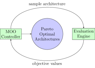
For a given search space, our goal is to find all the neural network architectures that offer the best trade-offs between multiple independent criteria. We formulate the search process as a multi-objective optimization (MOO) problem (Section 3.1) where each objective to optimize is an independent scalar value. We refer to Figure 1 for a general overview of the search process.
The MOO controller selects child networks with different architectures. The child networks are evaluated on multiple criteria by the Evaluation Engine. The resulting objective values are then used by the controller as feedback so it can generates better architectures over time. At each iteration, Dvolver keeps the hall of fame of the best architectures found so far.
3.1 Multi-objective optimization and Pareto dominance
We define the search space as the set of all feasible solutions and the objective space as the set of all possible values of the objective function . Dvolver searches for solutions by maximizing the objective function over with the total order relation defined next.
For a nontrivial multi-objective optimization problem, there is no solution that simultaneously optimizes all the objectives. In that case, the objective functions are said to be conflicting, and there exists a (possibly infinite) number of compromise solutions called Pareto-optimal solutions. The set of Pareto optimal outcomes is often called the Pareto front.
A simple approach to cope with multi-objective functions is to use scalarization which squashes all the objective functions into a single function falling back to single-objective optimization. While very simple in practice, this method suffers from many shortcomings such as (i) the difficulty to combine multiple unrelated criteria into a single value and (ii) inefficient sampling of the full Pareto front.
A much better solution is to use Pareto dominance partially ordered relation defined as follow: A solution Pareto-dominates a solution , if all objective values for are greater than the objective values for but a least one is strictly superior. A feasible solution is Pareto optimal, if it is not dominated by another solution. Without additional subjective preference information, all Pareto optimal solutions are considered equally good.
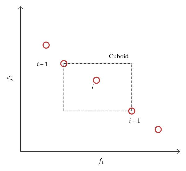
For the search process to be effective, it needs a totally ordered relation. Deb et al. (2002) defines the crowding distance value of a particular solution of point i as a measure of the objective space around i which is not occupied by any other solution in the population. Here, we simply calculate this quantity by estimating the perimeter of the cuboid (Figure 8) formed by using the nearest neighbors in the objective space as the vertices (See appendix A.2 for more details). In addition to the Pareto dominance criteria, the crowding distance defines the totally ordered relation used by Dvolver to perform its search process.
3.2 Search Algorithm
Dvolver evolves a population of individual architectures. At each iteration, the population evolves closer and closer toward the Pareto front, effectively sampling the full Pareto front in a single search process.
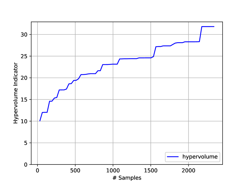
Our method starts by generating a random population and for each generation, it generates a child population, evaluates each child by training the networks for a few epochs on CIFAR-10 and selects the dominant architectures from the individuals (parents and children). The details of the algorithm is presented in appendix A.1. Algorithm convergence is monitored with the hypervolume indicator defined as the volume under the Pareto front (see A.3). In Algorithm 1, we present the Dvolver selection process inspired by NSGA-II (Deb et al., 2002).
-
•
individuals from parents’ population
-
•
individuals from offsprings’ population
-
•
selected individuals
At the end of an iteration, there are parents and children. We should select the best individuals to form the parents’ population for the next iteration. We compute the Pareto fronts for the individuals. The best fronts are considered first. If there are more than individuals in the best front, the first (with the help of the crowding distance) are selected and the selection ends. Otherwise, all the individuals from the front are selected and we carry on with the next best Pareto front until individuals are selected.
3.3 Search Space
Our work is based on the work of Zoph et al. (2017), in which network architecture is composed of two levels: a micro level architecture defined by parametrized cells composed of blocks and a macro architecture where those cells are stacked a predefined number of times, in order to create the final network. Figure 2(b) describes the macro architecture used for CIFAR-10 and ImageNet architectures.
There are two types of cells and Dvolver searches for both at the same time: (i) Normal Cell that returns a feature map of the same size as its input and (ii) Reduction Cell that returns a feature map of half the size of its input in the spatial dimensions.
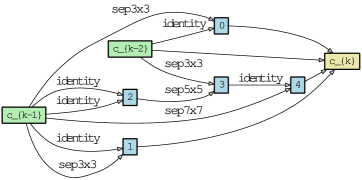
A cell is composed of blocks arranged in a Directed Acyclic Graph (DAG). Each block is a mapping of two input tensors to one output tensor and it can be represented by a 4-tuple, where specifies the input for the operation . The result of the two operations and are summed together to form the output of the block. A block can take its input from previous blocks, the previous cell or the previous previous cell . Unused blocks are concatenated in the depth dimension to form the final output of the cell.
Moreover, we noticed that the original NASNet search space can significantly benefit from extra connections from any given block, the previous cell and the previous previous cell to the final concatenation layer. In fact, these extra connections are already present but not described in the best models from Zoph et al. (2017), Real et al. (2018) and Liu et al. (2017a). Instead of adding manually these connections after the search process like in the previous works, Dvolver optimizes for these extra connections in addition to the 4 parameters for each block. In practice, our search space is the same as the one used by Zoph et al. (2017) but no manual intervention is needed. For , the total number of parameters for each type of cell is 20 parameters for the blocks and one list of indexes of extra connections.
Similar to the approach of Liu et al. (2017a), we simplify the search space and consider only the following operations:
-
•
identity
-
•
3x3 average pooling
-
•
3x3 max pooling
-
•
3x3 depthwise-separable conv
-
•
5x5 depthwise-separable conv
-
•
7x7 depthwise-separable conv
The total number of combinations for the defined search space is about taking into account symmetries and possible redundant connections. Note that our search space is larger than the one defined in Liu et al. (2017a) but we show in Section 4 that Dvolver is capable of finding competitive architectures faster.
4 Experiments and Results
Here we present the results for Dvolver with the method described in Section 3.1 and search space in Section 3.3. Searching for neural network architecture is done on CIFAR-10 (see Section 4.1) and optimization is performed with the validation accuracy and the number of floating points operations as independent objectives. In fact, Dvolver works by maximizing its objective functions, so in practice, the first objective function is the validation accuracy and the second is the . The best architectures are then fully trained on ImageNet (see Section 4.3).
4.1 Search Results
In this section, we describe our experiment to learn the Pareto front of convolutional cells for the search space described above. In particular, we conduct the search process on the CIFAR-10 dataset. We separate 5,000 images from the train set as a validation set used for architectures evaluation during the search process. We use a population of 32 individuals and a uniform mutation and a crossover probability of 0.1. Our preliminary studies shows that doubling or dividing by two these parameters does not have a large impact on the search process. We chose uniform operators instead of 1-point or 2-points operators to favor small architecture modifications: the different architectures parameters are modified independently of the other parameters.
The number of cells is set to 2 and use 32 convolution filters. Each sampled architecture is trained for 72 epochs with a batch size of 150 and a learning rate with a linear decay from 0.1 to 0.039. We evaluate the candidate architectures in parallel on multiple GPUs and the search process takes 50 GPU-days to find competitive architectures.
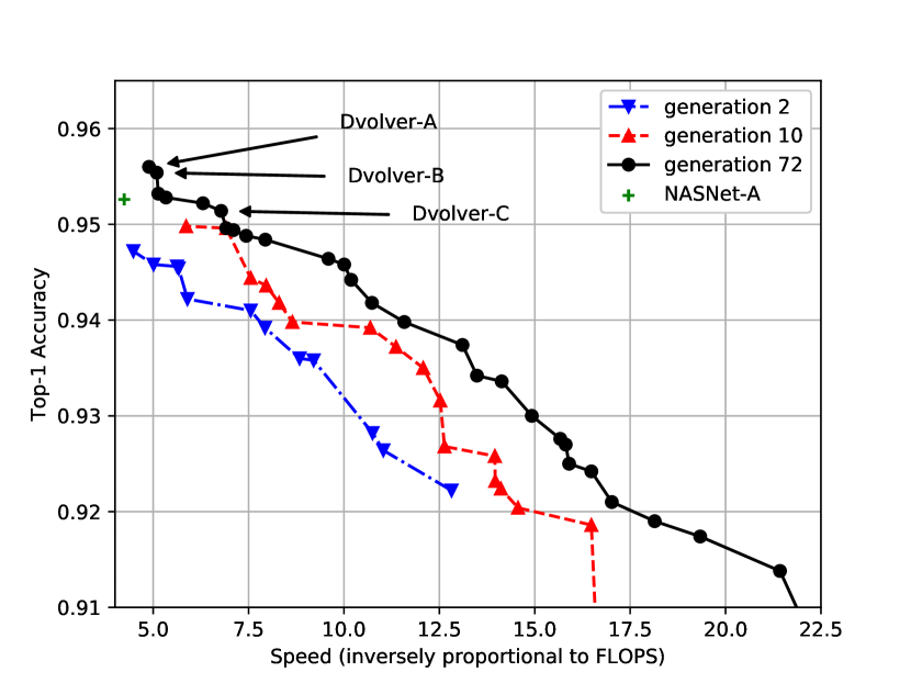
The Figure 3 shows the evolution of the hypervolume indicator as a function of the sampled architectures (Figure 3(a)) and the final Pareto front estimation with 2 intermediate fronts as an illustration of the evolution process. The horizontal segment in the Pareto front are particularly interesting. Cells situated on knees in the Pareto front are good trade-offs: for a small drop in accuracy there is a large gain in speed. Figure 3 shows how the Pareto front can be an appropriate tool when choosing a network architecture for a specific application.
Training all the Pareto optimal solutions in the front on ImageNet is very expensive and of limited interest in practice. Usually, when searching for efficient architecture for mobile, one is interested on an architecture with specific computational resources: it can be inference time or in our case the number of floating point operations. We manually select 3 architectures situated on the Pareto front knees that will be fully train on CIFAR-10 in Section 4.2 and on ImageNet in Section 4.3. They are called Dvolver-A, B and C. We choose and so that final neural networks have similar floating point budget to other neural networks in the competition for easy comparison.
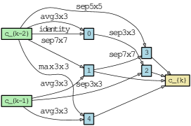
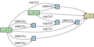
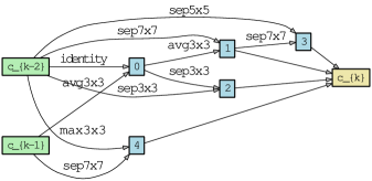
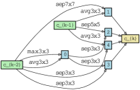
The detailed architectures of the cells for Dvolver-A, B and C are presented in the diagrams of Figure 4. We can see that, in most of them, additional connections (see Section 3.3) are present. This matches our observations during our preliminar experiments. On the contrary to previous works (Zoph et al., 2017), (Real et al., 2018) and (Liu et al., 2017a) where additional connections are added manually after the search process, our method is able to find them automatically.

4.2 Results on Cifar-10
We first present the results for the 3 architectures selected in section 4.1. We use the same preprocessing strategy as Zoph et al. (2017) namely the 3232 images are pad with zeros to 4040 images, then we select a random crop of 3232, apply random horizontal flip, perform random brightness and contrast variations and finally apply cutout preprocessing (Devries & Taylor, 2017).
First, we compare our method to single-objective methods taking into account only the test accuracy (see top half of Table 1). Parameters count is presented for reference. Dvolver is able to find network architectures with better test error than NASNet-A.
Then, we compare with multi-objectives methods (see bottom half of Table 1). While the search spaces are very different, Dvolver finds architectures with better test error than Dong et al. (2018) and is on part and even surpass the networks proposed by Elsken et al. (2018).
| Model | Top-1 Err.(%) | #Mult-Adds | #Parameters |
|---|---|---|---|
| NASNet-A (N=6, F=32) | 2.93 | 545M | 3.3M |
| Dvolver-A (N=5, F=36) | 2.9 | 505M | 3.17M |
| Dvolver-B (N=6, F=32) | 3.03 | 436M | 2.76M |
| Dvolver-C (N=6, F=32) | 3.04 | 315M | 2.08M |
| DPP-Net-PNAS | 4.36 | 1364M | 11.39M |
| DPP-Net-WS | 4.78 | 137M | 1.00M |
| DPP-Net-ES | 4.93 | 270M | 2.04M |
| DPP-Net-M | 5.84 | 59.27M | 0.45M |
| DPP-Net-Panacea | 4.62 | 63.5M | 0.52M |
| Lemonade Cell9 (V1) | 4.57 | - | 0.5M |
| Lemonade Cell9 (V2) | 3.69 | - | 1.1M |
| Lemonade Cell2 (V1) | 3.05 | - | 4.7M |
| Lemonade Cell2 (V2) | 2.58 | - | 13.1M |
4.3 Results on Imagenet
Dvolver-A, B and C cells found in Section 4.1 are fully trained for different combination of cells, number of normal cells and number of convolution cells on ImageNet following the training procedure found in Real et al. (2018). Input image size is set to 224x224 and each network is trained for 330 epochs. We use the standard inception preprocessing, train with rmsprop optimizer and exponential learning rate decay with initial learning rate of 2, 2.4 epochs per decay with 0.97 learning rate decay value and warmup for 3 epochs. The total batch size is 1600.
First, in Table 2, we select a few architectures with similar computational complexity as networks presented in Zoph et al. (2017) and show that we can find Pareto dominant architectures that can be more accurate and faster than architectures found with single objective optimization. Dvolver-A (N=4, F=44) has the same Top-1 accuracy of with less floating point operations than NASNet-A mobile. We also found two architectures with slightly more computations needs ( and more MACs) but with better Top-1 accuracy and respectively.
| Model | Top-1 Acc.(%) | Top-5 Acc.(%) | #Mult-Adds | #Parameters |
|---|---|---|---|---|
| NASNet-A (N=4, F=44) | 73.64 | 91.53 | 564M | 5.3M |
| Dvolver-A (N=3, F=48) | 73.14 | 91.37 | 493M | 4.3M |
| Dvolver-A (N=4, F=44) | 73.64 | 91.49 | 520M | 4.5M |
| Dvolver-A (N=4, F=48) | 74.81 | 92.15 | 607M | 5.25M |
| Dvolver-B (N=3, F=52) | 73.65 | 91.72 | 544M | 4.73M |
| Dvolver-C (N=3, F=44) | 70.24 | 89.58 | 317M | 2.76M |
| Dvolver-C (N=4, F=56) | 74.37 | 91.86 | 582M | 5.06M |
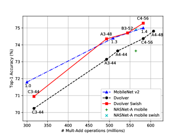
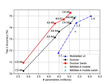
Inspired by the results of Ramachandran et al. (2017) on NASNet-A mobile, we replace all RELU activation functions by SWISH activation functions and compare our results with the best state-of-the-art architecture for mobile. We found that we can outperfom MobileNet-V2 in the high end mobile space with Top-1 accuracy for the same number of floating point operations but stay behind on low-end mobiles. Table 3 summarizes our findings:
| Model | Top-1 Acc.(%) | Top-5 Acc.(%) | #Mult-Adds | #Parameters |
|---|---|---|---|---|
| NASNet-A (4, 44, swish) | 74.9 | 92.4 | 564M | 5.3M |
| MobileNetV1-224 1.0 | 70.9 | 89.9 | 569M | 4.24M |
| MobileNetV1-224 0.75 | 68.4 | 88.2 | 317M | 2.59M |
| MobileNetV2-224 1.4 | 75.0 | 92.5 | 582M | 6.06M |
| MobileNetV2-224 1.3 | 74.4 | 92.1 | 509M | 5.34M |
| MobileNetV2-224 1.0 | 71.8 | 91.0 | 300M | 3.47M |
| MobileNetV2-224 0.75 | 69.8 | 89.6 | 209M | 2.61M |
| ShuffleNet (2x) | 70.9 | 89.8 | 524M | 5M |
| DPP-Net-Panacea | 74.02 | 91.79 | 523M | 4.8M |
| Dvolver-A (3, 48, swish) | 74.35 | 91.99 | 493M | 4.3M |
| Dvolver-B (3, 52, swish) | 74.70 | 92.33 | 544M | 4.73M |
| Dvolver-C (3, 44, swish) | 70.95 | 90.05 | 317M | 2.76M |
| Dvolver-C (4, 56, swish) | 75.28 | 92.32 | 582M | 5.06M |
There are a lot of different mobile devices with extreme computation resources diversity. To keep the discussion simple, we consider two tiers of devices: the low-end mobile market with devices with less than 400M Mult-Adds for a specific computation and a high-end tier with devices with higher performance.
Our best architectures are compared with the state-of-the-art architectures in Figure 5. In particular, we show that optimizing for multiple criteria including the number of floating operations, Dvolver finds architectures with better trade-offs than NASNet architectures. The poor performances at low operation count, show a weakness in the design of the NASNet search space which seems to be less efficient as a better tailored search space, design with low-end mobile device in mind.
4.4 Search Efficiency
An important result of our work is the computational resources needed to perform the architecture search. Dvolver finds the full Pareto front, on a much bigger search space, 3 times faster than PNAS (Liu et al., 2017a). Table 4 presents the computational resources needed to perform the automatic search process with different method found in the field.
| Method | GPU.days | Search Space Size (Approx.) |
|---|---|---|
| NASNet (Zoph et al., 2017) | 1800 | |
| PNAS (Liu et al., 2017a) | 150 | |
| AmoebaNet (Real et al., 2018) | 3150 | |
| Dvolver | 50 | |
| DPP-Net | 8 |
One explication for Dvolver speed compared to other method is that it actually generates a population of architectures and among them some are very fast (see Figure 3(b)). Intriguingly, these very fast architectures do not penalize the search process for the most accurate architectures. We think that the interaction between the different kind of individuals in the population is an essential property responsible for its effectiveness.
5 Conclusion
In this work, we propose a general method to search for Pareto-optimal neural architectures optimized for multiple criteria. In particular, we propose two novel cell structures. The first one achieves the same Top-1 accuracy on ImageNet as NASNet-A mobile with less floating point operations and the second one outperforms the best MobileNetV2 model by in Top-1 accuracy () for the same computational resources.
Our key contribution is the iterative population-based approach which approximates the Pareto front in a single search process. Our search method is efficient in terms of number of sampled architectures and computational resources. It performs the full search for the Pareto front in 50 GPU.days, 3 times faster than PNAS (Liu et al., 2017a) on a larger search space.
Our work is based on a few assumptions that can be discussed. First, it relies on CIFAR-10 as proxy for ImageNet in the search process. This has several weaknesses: It is very hard to distinguish different architectures on this dataset as the differences between architecture’s accuracies are very small and very noisy. In addtition, our method relies on the order to be conserved when transfering the architectures from CIFAR-10 to ImageNet and in practice it works but it is not always the case. Second, it is very expensive to fully train each candidate architecture from scratch even on CIFAR-10. To speedup the search process, we train for a few epochs with high learning rate and state that the ordering for this few epochs is the same as the one if all the architectures were fully trained. This is not always the case and it can inder the performance of the search process.
As a future work, we could apply our method on a different search space inspired by the lastest state-of-the-art mobile architectures to improve the performance on low-end mobile devices. Another way to improve our work is to enhance the selection phase by reducing the variance in the accuracy caused by the early stopping assumption.
References
- Baker et al. (2016) Bowen Baker, Otkrist Gupta, Nikhil Naik, and Ramesh Raskar. Designing neural network architectures using reinforcement learning. CoRR, abs/1611.02167, 2016. URL http://arxiv.org/abs/1611.02167.
- Brock et al. (2017) Andrew Brock, Theodore Lim, James M. Ritchie, and Nick Weston. SMASH: one-shot model architecture search through hypernetworks. ICML, abs/1708.05344, 2017. URL http://arxiv.org/abs/1708.05344.
- Chrabaszcz et al. (2017) Patryk Chrabaszcz, Ilya Loshchilov, and Frank Hutter. A downsampled variant of imagenet as an alternative to the CIFAR datasets. CoRR, abs/1707.08819, 2017. URL http://arxiv.org/abs/1707.08819.
- Deb et al. (2002) Kalyanmoy Deb, Samir Agrawal, Amrit Pratap, and T. Meyarivan. A fast and elitist multiobjective genetic algorithm: NSGA-II. IEEE Trans. Evolutionary Computation, 6(2):182–197, 2002. doi: 10.1109/4235.996017. URL https://doi.org/10.1109/4235.996017.
- Deng et al. (2009) Jia Deng, Wei Dong, Richard Socher, Li-Jia Li, Kai Li, and Fei-Fei Li. Imagenet: A large-scale hierarchical image database. In 2009 IEEE Computer Society Conference on Computer Vision and Pattern Recognition (CVPR 2009), 20-25 June 2009, Miami, Florida, USA, pp. 248–255. IEEE Computer Society, 2009. ISBN 978-1-4244-3992-8. doi: 10.1109/CVPRW.2009.5206848. URL https://doi.org/10.1109/CVPRW.2009.5206848.
- Devries & Taylor (2017) Terrance Devries and Graham W. Taylor. Improved regularization of convolutional neural networks with cutout. CoRR, abs/1708.04552, 2017. URL http://arxiv.org/abs/1708.04552.
- Dong et al. (2018) Jin-Dong Dong, An-Chieh Cheng, Da-Cheng Juan, Wei Wei, and Min Sun. DPP-Net: Device-aware Progressive Search for Pareto-optimal Neural Architectures. Technical report, 2018. URL https://arxiv.org/pdf/1806.08198.pdf.
- Elsken et al. (2018) Thomas Elsken, Jan Hendrik Metzen, and Frank Hutter. Efficient Multi-objective Neural Architecture Search via Lamarckian Evolution. 2018. URL http://arxiv.org/abs/1804.09081.
- Krizhevsky & Hinton (2009) Alex Krizhevsky and Geoffrey Hinton. Learning multiple layers of features from tiny images. Technical report, University of Toronto, 2009.
- Krizhevsky et al. (2017) Alex Krizhevsky, Ilya Sutskever, and Geoffrey E. Hinton. Imagenet classification with deep convolutional neural networks. Commun. ACM, 60(6):84–90, 2017. doi: 10.1145/3065386. URL http://doi.acm.org/10.1145/3065386.
- Lecun et al. (1998) Y. Lecun, L. Bottou, Y. Bengio, and P. Haffner. Gradient-based learning applied to document recognition. Proceedings of the IEEE, 86(11):2278–2324, 1998. ISSN 0018-9219. doi: 10.1109/5.726791. URL http://dx.doi.org/10.1109/5.726791.
- Liu et al. (2017a) Chenxi Liu, Barret Zoph, Jonathon Shlens, Wei Hua, Li-Jia Li, Li Fei-Fei, Alan L. Yuille, Jonathan Huang, and Kevin Murphy. Progressive neural architecture search. CoRR, abs/1712.00559, 2017a. URL http://arxiv.org/abs/1712.00559.
- Liu et al. (2017b) Hanxiao Liu, Karen Simonyan, Oriol Vinyals, Chrisantha Fernando, and Koray Kavukcuoglu. Hierarchical representations for efficient architecture search. CoRR, abs/1711.00436, 2017b. URL http://arxiv.org/abs/1711.00436.
- Liu et al. (2018) Hanxiao Liu, Karen Simonyan, and Yiming Yang. DARTS: differentiable architecture search. CoRR, abs/1806.09055, 2018. URL http://arxiv.org/abs/1806.09055.
- Pham et al. (2018) Hieu Pham, Melody Y. Guan, Barret Zoph, Quoc V. Le, and Jeff Dean. Efficient neural architecture search via parameter sharing. In Jennifer G. Dy and Andreas Krause (eds.), Proceedings of the 35th International Conference on Machine Learning, ICML 2018, Stockholmsmässan, Stockholm, Sweden, July 10-15, 2018, volume 80 of JMLR Workshop and Conference Proceedings, pp. 4092–4101. JMLR.org, 2018. URL http://proceedings.mlr.press/v80/pham18a.html.
- Precup & Teh (2017) Doina Precup and Yee Whye Teh (eds.). Large-Scale Evolution of Image Classifiers, volume 70 of Proceedings of Machine Learning Research, 2017. PMLR. URL http://proceedings.mlr.press/v70/real17a.html.
- Ramachandran et al. (2017) Prajit Ramachandran, Barret Zoph, and Quoc V. Le. Searching for activation functions. CoRR, abs/1710.05941, 2017. URL http://arxiv.org/abs/1710.05941.
- Real et al. (2018) Esteban Real, Alok Aggarwal, Yanping Huang, and Quoc V. Le. Regularized evolution for image classifier architecture search. CoRR, abs/1802.01548, 2018. URL http://arxiv.org/abs/1802.01548.
- Sandler et al. (2018) Mark Sandler, Andrew G. Howard, Menglong Zhu, Andrey Zhmoginov, and Liang-Chieh Chen. Inverted residuals and linear bottlenecks: Mobile networks for classification, detection and segmentation. CoRR, abs/1801.04381, 2018. URL http://arxiv.org/abs/1801.04381.
- Smithson et al. (2016) Sean C. Smithson, Guang Yang, Warren J. Gross, and Brett H. Meyer. Neural networks designing neural networks: Multi-objective hyper-parameter optimization. CoRR, abs/1611.02120, 2016. URL http://arxiv.org/abs/1611.02120.
- Springenberg et al. (2014) Jost Tobias Springenberg, Alexey Dosovitskiy, Thomas Brox, and Martin A. Riedmiller. Striving for simplicity: The all convolutional net. CoRR, abs/1412.6806, 2014. URL http://arxiv.org/abs/1412.6806.
- Sutskever et al. (2014) Ilya Sutskever, Oriol Vinyals, and Quoc V. Le. Sequence to sequence learning with neural networks. CoRR, abs/1409.3215, 2014. URL http://arxiv.org/abs/1409.3215.
- Xie & Yuille (2017) Lingxi Xie and Alan L. Yuille. Genetic CNN. In IEEE International Conference on Computer Vision, ICCV 2017, Venice, Italy, October 22-29, 2017, pp. 1388–1397. IEEE Computer Society, 2017. ISBN 978-1-5386-1032-9. doi: 10.1109/ICCV.2017.154. URL https://doi.org/10.1109/ICCV.2017.154.
- Ye-Hoon et al. (2017) kim Ye-Hoon, Reddy Bhargava, Yun Sojung, and Seo Chanwon. NEMO: Neuro-Evolution with Multiobjective Optimization of Deep Neural Network for Speed and Accuracy. ICML’17 AutoML Workshop, 2017.
- Zhong et al. (2017) Zhao Zhong, Junjie Yan, and Cheng-Lin Liu. Practical network blocks design with q-learning. CoRR, abs/1708.05552, 2017. URL http://arxiv.org/abs/1708.05552.
- Zoph & Le (2016) Barret Zoph and Quoc V. Le. Neural architecture search with reinforcement learning. CoRR, abs/1611.01578, 2016. URL http://arxiv.org/abs/1611.01578.
- Zoph et al. (2017) Barret Zoph, Vijay Vasudevan, Jonathon Shlens, and Quoc V. Le. Learning transferable architectures for scalable image recognition. CoRR, abs/1707.07012, 2017. URL http://arxiv.org/abs/1707.07012.
Appendix A Algorithm Details
A.1 Genetic Algorithm
Figure 6 shows the details of the genetic algorithm used by Dvolver. The optimization process looks for a global optimum of the fitness function. It operates on a population of individuals (each being a point in the search space). Each iteration (also called generation) consists in selecting individuals from the parents’ population, applying crossover (also known as recombination) and mutation operators to define a new offsprings’ population. Each offspring’s fitness function is then evaluated. In the end, the most fitted individuals are kept and become the parents’ population for the next generation.
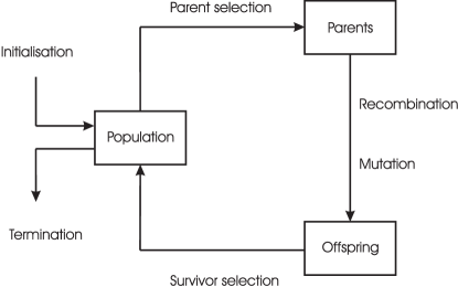
Individuals are points in the search space and genetic operators modify their vectorial representation. These transformations generate new individuals that inherit some attributes from their parents but also acquire new ones. We choose uniform crossover operator (see Figure 7(a)) which evaluates each component in the parents’ representation for exchange with a probability . It is particularly useful as it operates at the component level for fine-grained cell’s architecture modifications. For the same reason, we choose uniform mutation operator (see Figure 7(b)) which replaces the value of each component with a probability , by a uniform random value selected between the possible choices for that component.


The exploration of new individuals in the search space versus the exploitation of the best candidates are governed by the two parameters and , and are the unique two parameters for the genetic algorithm. Large value of allows to take larger steps across the problem domain, allowing the escape of local optimum. ’s value allows for small variations. It is possible to increase that value at the beginning of the search process to favor exploration then annealing that value as the population converge to a global optimum.
A.2 Crowding Distance
During the search process, it is necessary to compare every couple of candidates and be able to say which one is the best. Pareto dominance is only a partially ordered relation and it is not able by itself to rank two solutions on the Pareto front. For that purpose Deb et al. (2002) introduces the crowding distance to favor isolated solutions on the front. The idea is that it should help sampling the entire Pareto front. Pareto dominance and crowding distance defines a totally ordered relation that is independent of the ranges of the objective functions.
Figure 8 defines how the crowding distance is computed for each solution on the Pareto front. Red dots are part of the same Pareto front and the crowding distance for solution is the hypervolume of the cuboid. The crowding distance value of a solution provides an estimate of the density of solutions surrounding that solution.
A.3 Hypervolume indicator
With Multi-objective Optimization, an algorithm produces a set of points in the objective space as an estimation of the Pareto front. A quantitative measure is desired to estimate the closeness of the estimated data points to the true Pareto front. One of such measures is the hypervolume indicator, which gives the hypervolume between the estimated Pareto front (P) and a reference point (R).
The problem of interest is the maximization of all the objective functions when all the objectives are positives. In that case, the reference point can be set to zero and the hypervolume indicator is the k-area under the Pareto front surface (see Figure 9). is the hypervolume for the generations and is a monotonically increasing function with respect to the number of generations (or equivalently to the number of objective functions evaluations).
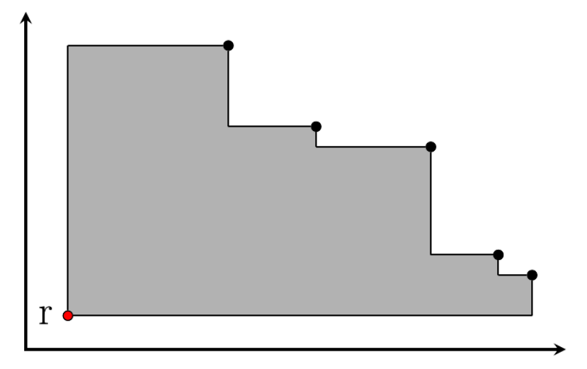
The hypervolume can be used to monitor the converge of the genetic algorithm: when the hypervolume indicator stops increasing, we can consider that we have reached convergence. In practice, It may be necessary to wait a little longer in case the genetic algorithm has been stuck in local optimum.