Charge symmetry violation in the determination of strangeness form factors

Abstract

The strange quark contributions to the electromagnetic form factors of the proton are ideal quantities to study the role of hidden flavor in the properties of the proton. This has motivated intense experimental measurements of these form factors. A major remaining source of systematic uncertainty in these determinations is the assumption that charge symmetry violation (CSV) is negligible. We use recent theoretical determinations of the CSV form factors and reanalyse the available parity-violating electron scattering data, up to $Q^{2}\sim 1$GeV². Our analysis considers systematic expansions of the strangeness electric and magnetic form factors of the proton. The results provide an update to the determination of strangeness over a range of $Q^{2}$ where, under certain assumptions about the effective axial form factor, an emergence of non-zero strangeness is revealed in the vicinity of $Q^{2}\sim 0.6\,{\rm GeV}^{2}$. Given the recent theoretical calculations, it is found that the current limits on CSV do not have a significant impact on the interpretation of the measurements and hence suggests an opportunity for a next generation of parity-violating measurements to more precisely map the distribution of strange quarks.

I Introduction

The desire for a complete understanding of the electromagnetic structure of the proton has led to significant efforts over the last two decades to determine the individual quark flavor contributions to the proton’s electromagnetic form factors. A significant challenge in this goal lies in determining the role played by non-valence or “hidden” quark flavors whose contributions arise only through fluctuations of the QCD vacuum. Being the lightest sea-only quark, strange quarks are anticipated to make the most significant contribution. Through an extensive experimental program of parity-violating electron scattering (PVES) Beise et al. (2005); Spayde et al. (2004); Maas et al. (2004); Baunack et al. (2009); Maas et al. (2005); Aniol et al. (2006a, 2004, b); Acha et al. (2007); Ahmed et al. (2012); Armstrong et al. (2005); Androic et al. (2010), strange quarks have been tagged by measuring the neutral-current form factors. The isolation of strangeness relies on the assumption of good charge symmetry, which has been one of the limiting factors in extending the experimental program to greater precision. In this work, we quantify the impact of charge symmetry violation (CSV) on the extraction of strangeness from a global analysis of the PVES measurements.

While earlier theoretical predictions of CSV in the proton’s electromagnetic form factors varied through several orders of magnitude Kubis and Lewis (2006); Wagman and Miller (2014); Miller et al. (2006); Lewis and Mobed (1999), a recent lattice QCD calculation Shanahan et al. (2015a) has determined that CSV in the proton’s electromagnetic form factors is significantly smaller than earlier expectations. Despite its importance for future measurements of parity violating electron-proton scattering and their subsequent interpretation as evidence of proton strangeness, the precise influence of this recent CSV constraint has not been throughly quantified. Hence, here we perform a global analysis of the full existing set of parity-violating (PV) asymmetry data with and without the constraint of CSV form factors. To achieve this task, we consider PVES data, obtained from experiments conducted with varying kinematics and targets, from SAMPLE Beise et al. (2005); Spayde et al. (2004), PVA4 Maas et al. (2004); Baunack et al. (2009); Maas et al. (2005), HAPPEX Aniol et al. (2006a, 2004, b); Acha et al. (2007); Ahmed et al. (2012), G0 Armstrong et al. (2005); Androic et al. (2010) and Q${}_{\text{weak}}$ Androic et al. (2013).

This paper is organised as follows: In section II, we describe the formalism of PVES, including PV asymmetries of the nucleon, helium-4 and the deuteron. Section III presents the parametrisation of strange quark form factor, while section IV is dedicated to a study of the CSV effects on strangeness form factor extraction. A brief summary is finally presented in section V.

II STRANGE FORM FACTORS AND PARITY-VIOLATING ELECTRON SCATTERING

Determining the strange electric and magnetic form factors experimentally requires a process where the weak and electromagnetic interactions interfere. This is achieved through PVES experiments Beck (1989); Mckeown (1989), whose leading-order amplitudes are shown in Fig. 1.

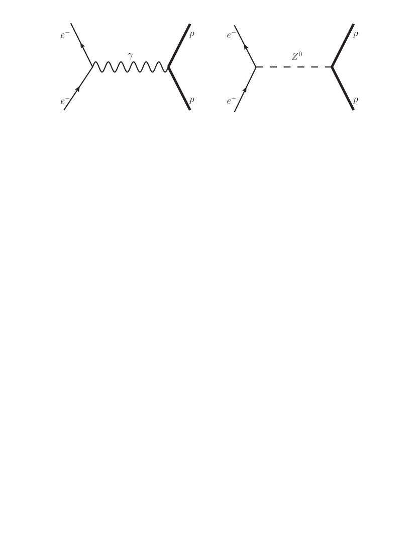
Figure 1: Total leading order amplitude for electron-nucleon scattering is the sum of the leading order electromagnetic and neutral current amplitudes.

Under the assumption of charge symmetry, the PV asymmetry in polarised $e$–$p$ scattering is given by Musolf et al. (1994)

$$A_{PV}^{p}=\Bigg{[}\frac{-G_{F}Q^{2}}{4\sqrt{2}\pi\alpha}\Bigg{]}(A^{p}_{V}+A^{p}_{s}+A^{p}_{A})\,.$$ (1)

where in terms of the proton’s electric $(G^{\gamma,p}_{E})$ and magnetic $(G^{\gamma,p}_{M})$ Sach’s form factors

$$A^{p}_{V}= (1-4\sin^{2}\hat{\theta}_{\text{w}})(1+R^{p}_{V})$$ (2)

$$-(1+R^{n}_{V})\frac{\epsilon G^{\gamma,p}_{E}G^{\gamma,n}_{E}+\tau G^{\gamma,p}_{M}G^{\gamma,n}_{M}}{\epsilon(G^{\gamma,p}_{E})^{2}+\tau(G^{\gamma,p}_{M})^{2}}\,,$$

$$A^{p}_{s}=-(1+R^{(0)}_{V})\frac{\epsilon G^{\gamma,p}_{E}G^{s}_{E}+\tau G^{\gamma,p}_{M}G^{s}_{M}}{\epsilon(G^{\gamma,p}_{E})^{2}+\tau(G^{\gamma,p}_{M})^{2}}\,,$$ (3)

and

$$A^{p}_{A}=\frac{-\epsilon^{\prime}(1-4\sin^{2}\hat{\theta}_{W})G^{\gamma,p}_{M}{\tilde{G}^{e,p}_{A}}}{\epsilon(G^{\gamma,p}_{E})^{2}+\tau(G^{\gamma,p}_{M})^{2}}.$$ (4)

are the proton’s vector form factor excluding strangeness $(A^{p}_{V})$, the proton’s strangeness vector form factor $(A^{p}_{s})$, and the interference of the proton’s magnetic vector and the axial vector form factors $(A^{p}_{A})$.

The electromagnetic form factors of the proton and neutron are denoted by $G_{E,M}^{\gamma}$, the strangeness vector form factors $G_{E,M}^{s}$, and the effective axial form factor $\tilde{G}_{A}^{p}$. The kinematic variables, which depend on the four-momentum transfer $Q^{2}=-q^{2}$ and the electron scattering angle $\theta$, are defined as

$$\tau=\frac{Q^{2}}{4M^{2}_{p}},$$ (5)

$$\epsilon=\frac{1}{1+2(1+\tau)\tan^{2}\frac{\theta}{2}},$$ (6)

and

$$\epsilon^{\prime}=\sqrt{\tau(1+\tau)(1-\epsilon^{2})},$$ (7)

where $M_{p}$, $\epsilon$ and $\epsilon^{\prime}$ are the proton’s mass, the virtual photon longitudinal polarization and the scattered energy, respectively. The standard model parameters: fine structure constant $\alpha$, Fermi coupling $G_{F}=1.16638\times 10^{-5}\,\mathrm{GeV}^{2}$, the weak mixing angle, $\sin^{2}\hat{\theta}_{W}=0.23129$, in the $\overline{\text{MS}}$ renormalization scheme, and the standard model radiative corrections, $R^{p}_{V}=-0.0513$ and $R^{n}_{V}=R^{(0)}_{V}=-0.0098$ are all obtained from the PDG  Tanabashi et al. (2018).

II.1 Helium-4 and Deuteron PV Asymmetries

The ⁴He nucleus is spin zero, parity even and isoscalar. Elastic electron scattering from ⁴He is an isoscalar $0^{+}\to 0^{+}$ transition and therefore allows no contributions from magnetic or axial-vector currents. Thus, the HAPPEX Collaboration has utilised a ⁴He target to directly extract the strange electric form factor Aniol et al. (2006a). Nuclear corrections are relevant for ⁴He and deuteron targets, more details about which can be found in Donnelly et al. (1989); Moreno and Donnelly (2014).

The theoretical asymmetry based on the assumption that isospin mixing can be neglected is written as Musolf et al. (1994)

$$A^{He}_{PV}= \Bigg{[}\frac{G_{F}Q^{2}}{4\sqrt{2}\pi\alpha}\Bigg{]}.\Bigg{[}(1-4\sin^{2}\theta_{\text{w}})(1+R^{p}_{V})-(1+R^{n}_{V})$$ (8)

$$+2\frac{-\big{(}1+R^{(0)}_{V}\big{)}G^{s}_{E}}{G^{p}_{E}+G^{n}_{E}}\Bigg{]}.$$

Corrections associated with isospin violations will be considered in Section IV.

The parity-violating asymmetries measured in quasi-elastic scattering from the deuteron have responses which involve the deuteron wavefunctions. For this analysis, we use directly the theoretical asymmetries as reported with original experimental measurements. Early results from SAMPLE have had minor modifications made to update for more recent radiative corrections and form factor parameterisations, as described in Ref. Young et al. (2006).

II.2 $\gamma Z$-exchange corrections to PVES

Leading electroweak corrections play a significant role in precision measurements of the strangeness contribution to the nucleon form factors Musolf and Holstein (1990); Musolf et al. (1994). In contrast to the formalism relevant to atomic parity violation experiments Marciano and Sirlin (1983), an energy-dependent correction arising from the $\gamma Z$ box diagram was highlighted by Gorchtein & Horowitz Gorchtein and Horowitz (2009). The size of this correction is particularly significant to the standard model test by the Q-weak Experiment Androić et al. (2018). Fortunately, the uncertainties arising from the underlying $\gamma Z$ interference structure functions can be reliably constrained Hall et al. (2013). These results have been further supported by direct measurement Wang et al. (2014).

The significance of the $\gamma Z$ box is somewhat less pronounced in the determination of strangeness. Nevertheless, for example, the correction makes about $\sim\tfrac{1}{2}$-sigma shift to the central value of the precise HAPPEX proton point at $Q^{2}\sim 0.1\,\mathrm{GeV}^{2}$. We incorporate the corrections reported by the constrained model of Ref. Hall et al. (2013), updated with the improved constraints of quark-hadron duality Hall et al. (2016), and a momentum dependence as proposed in Ref. Gorchtein et al. (2011). For completeness, a table of values is included in Appendix B.

II.3 Theoretical asymmetries

In this work, a set of all available PV asymmetry data up to $Q^{2}\sim 1\,$GeV², as summarised in Table 3, is analysed. Such a combined analysis of the world PV data requires a consistent treatment of the vector and axial form factors and radiative corrections. The theoretical asymmetry used in this analysis is written as

$$A_{Theory}=\eta_{0}+\eta^{p}_{A}\tilde{G}^{p}_{A}+\eta^{n}_{A}\tilde{G}^{n}_{A}+\eta_{E}G^{s}_{E}+\eta_{M}G^{s}_{M},$$ (9)

where the $\eta$’s, provided in Table 3, are calculated using the recent elastic form factor parameterisations of Ye et al. Ye et al. (2018) and current values for the standard model radiative corrections Tanabashi et al. (2018).

In this analysis, since the entire contribution is to be fit to data, we employ the effective axial form factors $\tilde{G}^{p,n}_{A}$ which implicitly includes both the axial radiative and anapole corrections. For these form factors, we employ a dipole form

$$\tilde{G}^{p,n}_{A}=\tilde{g}^{p,n}_{A}\bigg{(}1+\frac{Q^{2}}{M_{A}^{2}}\bigg{)}^{-2}\,,$$ (10)

with an axial dipole mass $M_{A}=1.026$ GeV, determined from neutrino scattering Bernard et al. (2002), common to both proton and neutron form factors. The normalisations $\tilde{g}^{p,n}$ are fit to the data, however since the isoscalar combination is very poorly determined, we choose to impose theoretical esimates based on an effective field theory (EFT) with vector-meson dominance (VMD) model to constrain this combination, $(\tilde{g}^{p}_{A}+\tilde{g}^{n}_{A})/2=-0.08\pm 0.26$ Zhu et al. (2000).

III Analysis framework

III.1 Taylor expansion

At low momentum transfers, a Taylor series expansion of the electromagnetic form factors in $Q^{2}$ is sufficient and minimises the model dependence. Given the sparsity and precision of the available data—up to $\sim 1\,\mathrm{GeV}^{2}$—we avoid introducing a specific model by first attempting to parameterise the strange electric and magnetic form factors $Q^{2}$ dependence by

$$G^{s}_{E} =\rho_{s}Q^{2}+\rho_{s}^{\prime}Q^{4}\,,$$

$$G^{s}_{M} =\mu_{s}+\mu_{s}^{\prime}Q^{2}\,.$$ (11)

III.2 $z$-expansion

A priori, one might not expect a Taylor expansion up to $\sim 1\,{\rm GeV}^{2}$ to be satisfactory. To provide an alternative functional form to the Taylor expansion, we also consider the $z$-expansion which offers improved convergence based on the analytic properties of the form factors Cutkosky and Deo (1968); Hill and Paz (2010); Epstein et al. (2014). We describe the momentum dependence of the strange form factors using the $z$-expansion, also to second (nontrivial) order:

$$G^{s}_{E}=\rho_{s,z}z+\rho_{s,z}^{\prime}z^{2},$$

$$G^{s}_{M}=\mu_{s}+\mu_{s,z}^{\prime}z,$$ (12)

where

$$z=\frac{\sqrt{t_{cut}+Q^{2}}-\sqrt{t_{cut}}}{\sqrt{t_{cut}+Q^{2}}+\sqrt{t_{cut}}}\,.$$ (13)

In our fits, we use choose $t_{cut}=(2m_{K})^{2}$, with the kaon mass $m_{K}=0.494$ GeV. In the absence of isospin violation, the cut formally starts at $9m_{\pi}^{2}$, but we assume that the strangeness contribution to the 3-pion state can be neglected. We note that, with the current experimental precision, there isn’t any significant sensitivity to the value of $t_{cut}$. To more easily facilitate the comparison with the two expansion forms, we report the simple Taylor expansion coefficients for each case. That is, for the $z$ fits, we translate the expansions back in the leading Taylor form, e.g. $\rho_{s}=dG^{s}_{E}/dQ^{2}|_{Q^{2}=0}$.

III.3 Charge symmetric results

Here we summarise the fit results under the assumption of exact charge symmetry. This provides a baseline with which to explore the implications of charge symmetry violation in the following section.

In this work we perform a global fit at leading order (LO) and at next leading order (NLO) of the strangeness form factor. Thus, the fitting procedure at LO considers four parameters, $\tilde{g}^{p}_{A}$, $\tilde{g}^{n}_{A}$, $\mu_{s}$ and $\rho_{s}$, while fitting at NLO considers an additional two parameters, $\mu^{\prime}_{s}$ and $\rho^{\prime}_{s}$.

The $\chi^{2}$ is calculated as

$$\chi^{2}=\sum_{i}\sum_{j}(m_{i}-t_{i})(V)^{-1}_{ij}(m_{j}-t_{j})\,,$$ (14)

where $m$ and $t$ denote the measurement and theory asymmetry respectively. The indicies $i$ and $j$ run over the data ensemble. The matrix $V$ represents the covariance error matrix defined as

$$(V)_{ij}=(\sigma^{uncor}_{i})^{2}\delta_{ij}+\sigma^{cor}_{i}\sigma^{cor}_{j}\,,$$ (15)

where $\sigma^{uncor}_{i}$ and $\sigma^{cor}_{i}$ are uncorrelated and correlated uncertainties of the $i^{\text{th}}$-measurement, respectively. We note that the correlated uncertainties are only relevant for the G0 experiment, where the forward Armstrong et al. (2005) and backward Androic et al. (2010) are treated as mutually independent. The goodness of fit is estimated from the reduced $\chi^{2}$ as

$$\chi^{2}_{red}=\chi^{2}/\text{d.o.f}\,,$$ (16)

with 33 and 31 degrees of freedom (d.o.f) for the LO and NLO fits, respectively. Note that with the isoscalar axial “charge” constrained, as described above, there are effectively 3(5) fit parameters in the LO(NLO) fits.

Table 1: The parameter values and $\chi^{2}$ obtained from previous PVES global fits Young et al. (2006); González-Jiménez et al. (2014); Young et al. (2007); Liu et al. (2007) and the current global analysis at LO for both Taylor and $z$-expansion form factor fits without constraints from CSV.

	$\rho_{s}$ [GeV-2]	$\mu_{s}$	$\chi^{2}_{red}$
YRCT(2006) Young et al. (2006)	$-0.06\pm 0.41$	0.12$\pm$0.55	1.3
YRCT(2007) Young et al. (2007)	$0.02\pm 0.18$	$-0.01\pm 0.25$	—
LMR(2007) Liu et al. (2007)	$-0.08\pm 0.16$	$0.29\pm 0.21$	1.3
GCD(2014) González-Jiménez et al. (2014)	0.26$\pm$0.16	$-0.26\pm 0.26$	1.3
Taylor	0.15$\pm$0.04	-0.12$\pm$0.04	1.1
$z$-exp.	0.18$\pm$0.05	-0.10$\pm$0.04	1.1

Table 2: The NLO parameters values and $\chi^{2}$ obtained from a previous global fit Young et al. (2006), where $Q^{2}<0.3$ GeV², and the current global analysis at NLO for both Taylor and $z$-expansion form factor fits without constraints from CSV.

	$\rho_{s}$ [GeV-2]	$\rho_{s}^{\prime}$ [GeV-4]	$\mu_{s}$	$\mu_{s}^{\prime}$ [GeV-2]	$\chi^{2}_{red}$
YRCT(2006) Young et al. (2006)	$-0.03\pm 0.63$	$-1.5\pm 5.8$	$0.37\pm 0.79$	$0.7\pm 6.8$	1.4
Taylor	0.07$\pm$0.14	0.14$\pm$0.22	-0.05$\pm$0.15	-0.11$\pm$0.23	1.23
$z$-exp.	0.08$\pm$0.17	0.19$\pm$0.37	-0.09$\pm$0.14	-0.06$\pm$0.29	1.26

We report the leading-order fit results in Table 1, with comparisons against previous work. The results are compatible with earlier work, though with significantly reduced uncertainty. This is due to both an updated list of measurements and the inclusion of the full range of $Q^{2}$ points in the fit. No appreciable difference is seen between the simple Taylor expansion and the $z$-expansion.

While the fit quality is reasonable, these simple leading-order fits are certainly anticipated to be too simple to describe these form factors over the full range $0\leq Q^{2}\lesssim 1.0\,\mathrm{GeV}^{2}$. As a result, the statistical uncertainties displayed are not representative of the current knowledge of the strange form factors. We hence allow for more variation in the $Q^{2}$ dependence by extending the fits to next-leading order, Eqs. (III.1) and (III.2). Results are shown in Table 2. Curiously the additional fit parameters are unable to make significant improvement to the $\chi^{2}$ and the reduced $\chi^{2}$ very marginally increases for the NLO fit.

Although the data do not support any structure offered by the NLO fits, we prefer the results at this order as being better representative of the uncertainties of the strangeness form factors, while offering some degree of smoothing of the underlying data. We note that given the clustering of the underlying data set, the separation of the electric and magnetic strange form factors are only most reliable at the discrete momentum transfers near $Q^{2}\sim 0.1,0.2$ and $0.6\,\mathrm{GeV}^{2}$. As such, the NLO fits are roughly fitting 3 data points with 2 parameters for each form factor. Attempting further higher order will just amount to over-fitting the statistical fluctuations of the data set.

The comparison between the leading and next-to-leading order fits for the Taylor expansion are shown in Figure 2. The corresponding $z$-expansion results are very similar. In Fig. 3 we show the NLO $z$-expansion parameterisation of the separated electric and magnetic form factors and compare with recent lattice QCD results Shanahan et al. (2015b); Sufian et al. (2017). Here we observe excellent agreement between our strangeness determination based on PVES data and lattice QCD results over the full $Q^{2}$ range. These are also compatible with earlier lattice Green et al. (2015) and lattice-constrained Leinweber et al. (2005, 2006); Wang et al. (2009) results. Interestingly, we note that the experimental results are showing some support for a non-vanishing strangeness electric form factor in the vicinity of $Q^{2}\sim 0.6\,\mathrm{GeV}^{2}$. Given the lack of sensitivity to the choice of functional form, we adopt the $z$-expansion at NLO as our preferred fit for the following discussions.

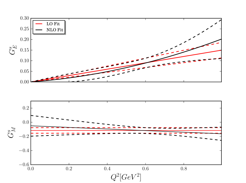
Figure 2: The extracted strange electric and magnetic form factors from a global fit up to $Q^{2}\sim 1$ GeV² using the Taylor expansions in Eq. (III.1). The red (black) solid curve shows the LO (NLO) fit and bound shown by the dotted curves.

Figure 3: The extracted strange electric and magnetic form factors from global fit up to $Q^{2}\sim 1$ GeV² with using the NLO $z$-expansion in Eq. (III.2). A comparison with recent lattice QCD results is shown where the green square (errors bars smaller than the symbol) corresponds to the result of $G^{s}_{M}$($Q^{2}=0.1$ GeV²) Sufian et al. (2017) and the magenta squares are $G^{s}_{M}$ and $G^{s}_{E}$ at $Q^{2}=0.17,\ 0.62$ and 0.88 GeV² Shanahan et al. (2015b).

The preceeding discussion has focussed on the separation of the electric and magnetic strangeness form factors. Given the high degree of correlation in the measurements, it is instructive to display the joint confidence intervals. Fig. 4 displays the 95$\%$ confidence level ellipses for the different values of $Q^{2}=0.1,0.23$ and $0.63\,\mathrm{GeV}^{2}$ for the NLO $z$-expansion fit.

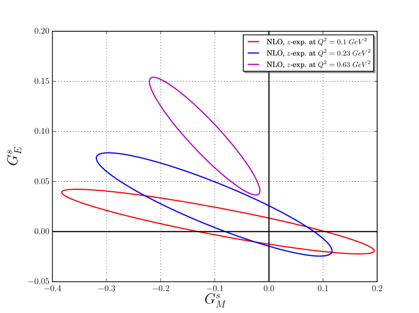
Figure 4: 95% confidence level ellipses for the electric and magnetic strangeness form factors using the NLO $z$-expansion in Eq. (III.2) for three $Q^{2}$ values 0.1, 0.23, 0.63 GeV².

At the low $Q^{2}$ values, we observe that the strangeness form factors are compatible with zero at the 95% CL, with a marginal preference for positive values of strange electric form factor and negative values of the magnetisation — as seen earlier in Refs. Young et al. (2007); Moreno et al. (2015).

At $Q^{2}=0.63\,\mathrm{GeV}^{2}$, there appears a clear signal for nonzero strangeness, with a negative $G_{M}^{s}$ and positive $G_{E}^{s}$. In contrast to earlier work that has suggested vanishing strangeness at this $Q^{2}$ Androic et al. (2010); Ahmed et al. (2012), the dominant difference in the present work is the treatment of the axial/anapole form factor. As described, the isoscalar combination is constrained by the EFT and VMD estimate of Zhu et al. Zhu et al. (2000), while the isovector combination is determined by the data. The best fit—for $z$-expansion at NLO—results in $\tilde{g}_{A}^{p}=-0.67\pm 0.25$, which is less negative than the zero-anapole approximation. As a consequence, the data-driven fit drives the back-angle G0 results to be more consistent with a negative $G_{M}^{s}$. Under these assumptions for the effective axial form factor, we see $G_{E}^{s}\sim 0.1$, which—with the strange charge factor included—is on the order of 10% of the proton electric form factor at this momentum transfer. Given the smallness of the strange form factors determined in direct lattice calculations Green et al. (2015); Sufian et al. (2017), the result seen here suggests a future investigation of the anapole “charge” and $Q^{2}$ dependence is warranted.

IV Sensitivity to Charge symmetry violation

IV.1 CSV in asymmetries

In this section we study the effects of charge symmetry violation on our results, i.e. we no longer have a relationship between the individual quark flavour contributions to the proton and neutron form factors

$$G^{p,u}_{E,M} \neq G^{n,d}_{E,M},$$

$$G^{p,d}_{E,M} \neq G^{n,u}_{E,M}.$$

We follow standard notation and define the CSV form factors as

$$G^{CSV}_{E,M}=\frac{2}{3}(G^{p,d}_{E,M}-G^{n,u}_{E,M})-\frac{1}{3}(G^{p,u}_{E,M}-G^{n,d}_{E,M})\,.$$ (17)

In order to explore the impact of CSV, we need to modify the neutral weak from factors to explicitly include a CSV term

$$G_{E,M}^{Z,p}= (1-4\sin^{2}\hat{\theta}_{W})(1+R^{p}_{V})G^{\gamma,p}_{E,M}$$

$$-(1+R^{n}_{V})G^{\gamma,n}_{E,M}-(1+R^{(0)}_{V})G^{s}_{E,M}$$ (18)

$$-(1+R^{n}_{V})G^{CSV}_{E,M},$$

where the $Q^{2}$-dependence of each form factor has been dropped for clarity. The CSV form factor can be expressed as a simple Taylor expansion in $Q^{2}$

$$G^{CSV}_{E,M}(Q^{2})=G^{CSV}_{E,M}(0)-\rho^{CSV}_{E,M}Q^{2}+\mathcal{O}(Q^{4}),$$ (19)

with $G^{CSV}_{E}$ set to zero at $Q^{2}=0$ due to charge conservation.

Regarding the theoretical asymmetry given in Eq. 9, we note that $\eta_{0}$ will receive a correction due to the CSV form factor. Hence

$$A_{Theory}=\eta^{CSV}_{0}+\eta^{p}_{A}\tilde{G}^{p}_{A}+\eta^{n}_{A}\tilde{G}^{n}_{A}+\eta_{E}G^{s}_{E}+\eta_{M}G^{s}_{M}\,,$$ (20)

where $\eta^{CSV}_{0}=\eta_{0}+\eta^{CSV}_{E}G^{CSV}_{E}+\eta^{CSV}_{M}G^{CSV}_{M}$, with

$$\eta^{N}_{{}_{CSV,E}}=\Big{[}\frac{G_{F}Q^{2}}{4\sqrt{2}\pi\alpha}\Big{]}.\Big{[}\frac{(1+R^{n}_{V})\epsilon G^{\gamma,N}_{E}}{\epsilon(G^{\gamma,N}_{E})^{2}+\tau(G^{\gamma,N}_{M})^{2}}\Big{]}\,,$$ (21)

$$\eta^{N}_{{}_{CSV,M}}=\Big{[}\frac{G_{F}Q^{2}}{4\sqrt{2}\pi\alpha}\Big{]}.\Big{[}\frac{(1+R^{n}_{V})\tau G^{\gamma,N}_{M}}{\epsilon(G^{\gamma,N}_{E})^{2}+\tau(G^{\gamma,N}_{M})^{2}}\Big{]}\,.$$ (22)

In the case of the PV asymmetry of ⁴He, we should consider nuclear CSV, which we denote $F^{CSV}$, in addition to CSV at nucleon level, $G^{CSV}_{E}$. In this case, $\eta^{CSV}_{0}$ can therefore be written as

$$\eta^{CSV}_{0}=\eta_{0}-2F^{CSV}+4\frac{\left(1+R^{n}_{V}\right)G^{CSV}_{E}}{G^{p}_{E}+G^{n}_{E}}\,,$$ (23)

where in the notation of Viviani et al. (2007), $F^{CSV}\equiv F^{(1)}(q)/F^{(0)}(q)=-0.00157$ is used to calculate $\eta^{CSV}_{0}$ for the theoretical PV asymmetry of ⁴He at $Q^{2}=0.077$ and 0.091 GeV².

IV.2 CSV Theoretical Works

To include effects of charge symmetry violation in our determination of the strangeness form factors, we consider three different calculations of the CSV form factors. The first work we consider is from Kubis and Lewis Kubis and Lewis (2006), denoted by “K$\&$L CSV”. They used effective field theory, supplemented with resonance saturation to estimate the relevant contact term — where the CSV is largely driven by $\rho-\omega$ mixing. To accomplish this, they employ a large $\omega$-nucleon coupling constant $g_{\omega}\sim 42$ taken from dispersion analysis. Combining this estimate with calculations in HB$\chi$PT and infrared regularised baryon chiral perturbation theory, K$\&$L predicted a CSV magnetic moment contribution $G^{CSV}_{M}(0)\equiv k^{u,d}=0.025\pm 0.020$, which includes an uncertainty arising from the resonance parameter. For the CSV slope parameters, K$\&$L found $\rho^{CSV}_{M}=-0.08\pm 0.06$ GeV^-2 and $\rho^{CSV}_{E}=-0.055\pm 0.015$ GeV^-2. We take these values as our first estimate of the CSV form factors.

The second theoretical calculation of CSV we consider is from Wagman and Miller Wagman and Miller (2014), denoted by “W$\&$M CSV”. In their work, they used relativistic chiral perturbation theory with a more realistic $\omega$-nucleon coupling i.e. $g_{\omega}\sim 10$. That study reported values of $G^{CSV}_{M}(0)=0.012\pm 0.003$, $\rho^{CSV}_{M}=0.015\pm 0.010$ GeV^-2 and $\rho^{CSV}_{E}=-0.018\pm 0.003$ GeV^-2.

The third determination of the CSV form factor that we employ is based on an analysis of lattice QCD results Shanahan et al. (2015a), that we refer to as “Lattice CSV”. The lattice study found significantly smaller values of the magnetic and electric CSV form factors compared to the previous two estimates. To study the effect of the CSV form factors obtained from lattice QCD, we summarise the results of Ref. Shanahan et al. (2015a) by $G^{CSV}_{M}=0.0\pm 0.001$ and $\rho^{CSV}_{E}=0.0\pm 0.001\,\mathrm{GeV}^{-2}$.

IV.3 Strangeness with CSV

In order to propagate the uncertainties, we extend the covariance matrix above, Eq. (15), to include a correlated uncertainty associated with the theoretical estimates of CSV. For each theoretical description, we reanalyse the entire data set and present in Fig. 5 our determination of the strange magnetic moment $\mu_{s}$ (left) and strange electric radius $\rho_{s}$ (right). Since the Lattice CSV form factors are zero with a negligible uncertainty, they are consistent with the “No CSV” results. We also find no visible impact on $\mu_{s}$ and $\rho_{s}$ from the inclusion of the W$\&$M CSV form factors. Finally, when estimating the CSV form factors by the K$\&$L parameters, we observe only small shifts in the central value of the strangeness magnetic moment. Nevertheless, even the “worst case” scenario of K$\&$L doesn’t appreciably affect the NLO fits.

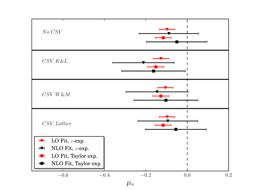
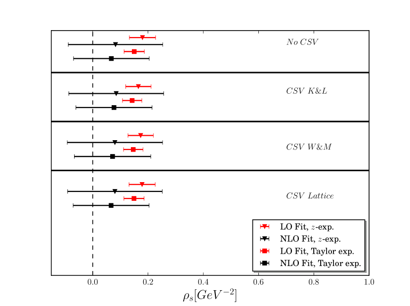
Figure 5: Comparison of determinations obtained from the present work with and without CSV for the strange magnetic moment $\mu_{s}$ (left) and strange electric radius $\rho_{s}$(right).

V conclusion

We have presented a complete global analysis of all PVES asymmetry data for the proton, ⁴He and deuterium. We have investigated the $\gamma Z$ exchange correction and the effect that CSV form factors have on the extraction of strange quark contribution. Including $\gamma Z$ box contribution in the analysis leads to small increases in the magnitude of the central values of $\mu_{s}$ and $\rho_{s}$ when compared to results obtained without constraints from $\gamma Z$-exchange. CSV results considered in this work have tiny effects on the central values of the strangeness parameters, with the largest effect, while still small, coming from the inclusion of CSV form factors as provided by Kubis and Lewis Kubis and Lewis (2006). Our results favour non-zero values for the strangeness magnetic moment and electric radius, with the most significant constraints coming from the LO fits using a Taylor expansion for the strangeness form factors. Finally, in order to examine the model dependence of employing a Taylor expansion in our analysis, we also included fits using the $z$-expansion which were found to be in agreement.

The latest theory estimates on CSV are small — indeed small enough that they would not cloud the interpretation of future precision strangeness measurements. However, we note that the back-angle measurements do exhibit sensitivity to the effective axial form factor, presenting an opportunity for future investigation. The combined efforts to improve the resolution of strangeness, and reveal the structure of the anapole form factor offer the potential to establish a precision era of QCD and the nucleon. While further advancing the understanding of the mechanisms underlying nonperturbative QCD, such work will serve to gain further confidence in the use of lattice QCD for precision constraints in tests of the standard model.

Appendix A Parity violating asymmetries

Table 3 lists the asymmetries and their dependence on the leading unknown hadronic structure for all existing PVES experiments.

Table 3: Values of $\eta_{i}$, appearing in Eq. 9, which describe the theoretical asymmetry for each experiment (in partsper-million). $A^{phys}$ and $\delta A$ are the measured asymmetry and the corresponding uncertainty respectively where the statistic ans systematic error have been added in quadrature. While $\delta A_{cor}$ is the correlated error in the G0 experiment Armstrong et al. (2005); Androic et al. (2010).

Experiment	Target	$Q^{2}$	$\theta$	$E$	$\eta_{0}$	$\eta^{p}_{A}$	$\eta^{n}_{A}$	$\eta_{E}$	$\eta_{M}$	$A^{phys}$	$\delta A$	$\delta A_{cor}$	Ref.
SAMPLE	d	0.038	144	0.11	-2.13	0.46	-0.30	1.16	0.28	-3.51	0.81	0	Beise et al. (2005)
SAMPLE	d	0.091	144	0.18	-7.02	1.04	-0.65	1.63	0.77	-7.77	1.03	0	Beise et al. (2005)
SAMPLE	p	0.1	144	0.2	-5.50	1.57	0	2.11	3.45	-5.61	1.11	0	Spayde et al. (2004)
HAPPEX	p	0.477	12.3	3.35	-15.82	1.13	0	55.65	23	-15.05	1.13	0	Aniol et al. (2004)
PVA4	p	0.230	35.3	0.85	-5.78	0.88	0	22.45	5.08	-5.44	0.60	0	Maas et al. (2004)
PVA4	p	0.108	35.4	0.57	-1.82	0.26	0	10.07	1.05	-1.36	0.32	0	Maas et al. (2005)
G0	p	0.122	6.68	3.03	-1.93	0.06	0	11.94	1.17	-1.51	0.49	0.18	Armstrong et al. (2005)
G0	p	0.128	6.84	3.03	-2.08	0.06	0	12.58	1.30	-0.97	0.46	0.17	Armstrong et al. (2005)
G0	p	0.136	7.06	3.03	-2.28	0.07	0	13.43	1.47	-1.30	0.45	0.17	Armstrong et al. (2005)
G0	p	0.144	7.27	3.03	-2.48	0.08	0	14.29	1.66	-2.71	0.47	0.18	Armstrong et al. (2005)
G0	p	0.153	7.5	3.03	-2.73	0.09	0	15.27	1.89	-2.22	0.51	0.21	Armstrong et al. (2005)
G0	p	0.164	7.77	3.03	-3.03	0.11	0	16.49	2.19	-2.88	0.54	0.23	Armstrong et al. (2005)
G0	p	0.177	8.09	3.03	-3.41	0.13	0	17.93	2.58	-3.95	0.50	0.20	Armstrong et al. (2005)
G0	p	0.192	8.43	3.03	-3.87	0.15	0	19.63	3.07	-3.85	0.53	0.19	Armstrong et al. (2005)
G0	p	0.210	8.84	3.03	-4.45	0.19	0	21.69	3.72	-4.68	0.54	0.21	Armstrong et al. (2005)
G0	p	0.232	9.31	3.03	-5.20	0.23	0	24.25	4.62	-5.27	0.59	0.23	Armstrong et al. (2005)
G0	p	0.262	9.92	3.03	-6.29	0.31	0	27.82	6.03	-5.26	0.53	0.17	Armstrong et al. (2005)
G0	p	0.299	10.63	3.03	-7.73	0.42	0	32.33	8.06	-7.72	0.80	0.35	Armstrong et al. (2005)
G0	p	0.344	11.45	3.03	-9.61	0.58	0	37.97	11.01	-8.40	1.09	0.52	Armstrong et al. (2005)
G0	p	0.410	12.59	3.03	-12.60	0.87	0	46.50	16.34	-10.25	1.11	0.55	Armstrong et al. (2005)
G0	p	0.511	14.2	3.03	-17.61	1.49	0	60.11	27.01	-16.81	1.73	1.50	Armstrong et al. (2005)
G0	p	0.631	15.98	3.03	-24.05	2.52	0	77.05	44.07	-19.96	1.69	1.31	Armstrong et al. (2005)
G0	p	0.788	18.16	3.03	-33.08	4.45	0	100.26	74.55	-30.83	3.16	2.59	Armstrong et al. (2005)
G0	p	0.997	20.9	3.03	-45.78	8.32	0	132.55	131.72	-37.93	11.55	0.52	Armstrong et al. (2005)
HAPPEX	He4	0.091	6.0	2.91	-7.52	0	0	-20.22	0	-6.72	0.87	0	Aniol et al. (2006a)
HAPPEX	p	0.099	6.0	3.03	-1.41	0.04	0	9.54	0.76	-1.14	0.25	0	Aniol et al. (2006b)
HAPPEX	He4	0.077	6.0	2.67	-6.37	0	0	-16.58	0	-6.40	0.26	0	Acha et al. (2007)
HAPPEX	p	0.109	6.0	3.18	-1.63	0.04	0	10.58	0.93	-1.58	0.13	0	Acha et al. (2007)
PVA4	p	0.22	144.5	0.31	-13.31	3.47	0	2.88	11.13	-17.23	1.21	0	Baunack et al. (2009)
G0	p	0.221	110	0.35	-10.61	2.73	0	9.37	8.93	-11.25	0.9	0.43	Androic et al. (2010)
G0	d	0.221	110	0.35	-15.25	2.05	-1.38	7.63	2.21	-16.93	0.91	0.21	Androic et al. (2010)
G0	p	0.628	110	0.68	-36.91	11.91	0	19.71	62.25	-45.9	2.53	1.0	Androic et al. (2010)
G0	d	0.628	110	0.68	-50.72	8.46	-5.66	16.63	14.62	-55.5	3.86	0.7	Androic et al. (2010)
HAPPEX	p	0.624	13.7	3.48	-23.54	2.12	0	76.59	42.76	-23.8	0.86	0	Ahmed et al. (2012)
PVA4	d	0.224	145	0.31	-18.65	2.50	-1.68	2.17	2.67	-20.11	1.35	0	Balaguer Ríos et al. (2016)
Qweak	p	0.025	7.9	1.16	-0.22	0.006	0	2.27	0.05	-0.279	0.05	0	Androic et al. (2013)

Appendix B Energy dependence of the $\gamma$–$Z$ box

To incorporate the effect induced by the energy-dependent component of the $\gamma$–$Z$ box radiative correction, the measured PV asymmetries given in Eq. (1) are modified by

$$A^{p}_{PV\,corr}=A^{p}_{PV}-\left[\frac{-G_{F}Q^{2}}{4\sqrt{2}\pi\alpha}\right]\square_{\gamma Z}(E,Q^{2})\ .$$ (24)

The forward (or vanishing momentum transfer) limit of this box are taken from Ref. Hall et al. (2016), which extends Ref. Hall et al. (2013) to also incoporate duality constraints. To estimate the momentum transfer dependence, we adopt the model suggested by Gorchtein et al. Gorchtein et al. (2011):

$$\square_{\gamma Z}(E,Q^{2})=\square_{\gamma Z}(E,0)\frac{\exp\left(-BQ^{2}/2\right)}{F_{1}^{p}(Q^{2})}\,,$$ (25)

with slope parameter estimated to be $B=7\pm 1\,\mathrm{GeV}^{2}$, and $F_{1}^{p}$ the electromagnetic Dirac form factor of the proton. The numerical values used in this work are summarised in Table 4.

Table 4: The $\square_{\gamma Z}(E)\ \big{(}\times 10^{-3}\big{)}$ corrections evaluated for the measured proton PV asymmetry $A^{p}_{PV}$ at forward angles.

Experiment	$Q^{2}$ (GeV2)	$E$ (GeV)	$\square_{\gamma Z}(E)\ \big{(}\times 10^{-3}\big{)}$
Qweak	0.025	1.165	5.120 $\pm$ 0.671
HAPPEx	0.099	3.030	7.205 $\pm$ 0.701
PVA4	0.108	0.570	2.843 $\pm$ 0.580
HAPPEx	0.109	3.180	7.250 $\pm$ 0.713
G0	0.122	3.030	6.969 $\pm$ 0.722
G0	0.128	3.030	6.907 $\pm$ 0.728
G0	0.136	3.030	6.825 $\pm$ 0.737
G0	0.144	3.030	6.742 $\pm$ 0.745
G0	0.153	3.030	6.648 $\pm$ 0.754
G0	0.164	3.030	6.534 $\pm$ 0.766
G0	0.177	3.030	6.398 $\pm$ 0.780
G0	0.192	3.030	6.243 $\pm$ 0.795
G0	0.210	3.030	6.056 $\pm$ 0.814
PVA4	0.230	0.850	3.257 $\pm$ 0.610
G0	0.232	3.030	5.831 $\pm$ 0.834
G0	0.262	3.030	5.527 $\pm$ 0.859
G0	0.299	3.030	5.161 $\pm$ 0.885
G0	0.344	3.030	4.733 $\pm$ 0.905
G0	0.410	3.030	4.143 $\pm$ 0.917
HAPPEx	0.477	3.350	3.749 $\pm$ 0.943
G0	0.511	3.030	3.340 $\pm$ 0.898
HAPPEx	0.624	3.480	2.740 $\pm$ 0.881
G0	0.631	3.030	2.547 $\pm$ 0.831
G0	0.788	3.030	1.753 $\pm$ 0.706
G0	0.997	3.030	1.038 $\pm$ 0.525

References

- Beise et al. (2005) E. J. Beise, M. L. Pitt, and D. T. Spayde, Prog. Part. Nucl. Phys. 54, 289 (2005), arXiv:nucl-ex/0412054 [nucl-ex] .
- Spayde et al. (2004) D. T. Spayde et al. (SAMPLE), Phys. Lett. B583, 79 (2004), arXiv:nucl-ex/0312016 [nucl-ex] .
- Maas et al. (2004) F. E. Maas et al. (A4), Phys. Rev. Lett. 93, 022002 (2004), arXiv:nucl-ex/0401019 [nucl-ex] .
- Baunack et al. (2009) S. Baunack et al., Phys. Rev. Lett. 102, 151803 (2009), arXiv:0903.2733 [nucl-ex] .
- Maas et al. (2005) F. E. Maas et al., Phys. Rev. Lett. 94, 152001 (2005), arXiv:nucl-ex/0412030 [nucl-ex] .
- Aniol et al. (2006a) K. A. Aniol et al. (HAPPEX), Phys. Rev. Lett. 96, 022003 (2006a), arXiv:nucl-ex/0506010 [nucl-ex] .
- Aniol et al. (2004) K. A. Aniol et al. (HAPPEX), Phys. Rev. C69, 065501 (2004), arXiv:nucl-ex/0402004 [nucl-ex] .
- Aniol et al. (2006b) K. A. Aniol et al. (HAPPEX), Phys. Lett. B635, 275 (2006b), arXiv:nucl-ex/0506011 [nucl-ex] .
- Acha et al. (2007) A. Acha et al. (HAPPEX), Phys. Rev. Lett. 98, 032301 (2007), arXiv:nucl-ex/0609002 [nucl-ex] .
- Ahmed et al. (2012) Z. Ahmed et al. (HAPPEX), Phys. Rev. Lett. 108, 102001 (2012), arXiv:1107.0913 [nucl-ex] .
- Armstrong et al. (2005) D. S. Armstrong et al. (G0), Phys. Rev. Lett. 95, 092001 (2005), arXiv:nucl-ex/0506021 [nucl-ex] .
- Androic et al. (2010) D. Androic et al. (G0), Phys. Rev. Lett. 104, 012001 (2010), arXiv:0909.5107 [nucl-ex] .
- Kubis and Lewis (2006) B. Kubis and R. Lewis, Phys. Rev. C74, 015204 (2006), arXiv:nucl-th/0605006 [nucl-th] .
- Wagman and Miller (2014) M. Wagman and G. A. Miller, Phys. Rev. C89, 065206 (2014), [Erratum: Phys. Rev.C91,no.1,019903(2015)], arXiv:1402.7169 [nucl-th] .
- Miller et al. (2006) G. A. Miller, A. K. Opper, and E. J. Stephenson, Ann. Rev. Nucl. Part. Sci. 56, 253 (2006), arXiv:nucl-ex/0602021 [nucl-ex] .
- Lewis and Mobed (1999) R. Lewis and N. Mobed, Phys. Rev. D59, 073002 (1999), arXiv:hep-ph/9810254 [hep-ph] .
- Shanahan et al. (2015a) P. E. Shanahan, R. Horsley, Y. Nakamura, D. Pleiter, P. E. L. Rakow, G. Schierholz, H. St uben, A. W. Thomas, R. D. Young, and J. M. Zanotti, Phys. Rev. D91, 113006 (2015a), arXiv:1503.01142 [hep-lat] .
- Androic et al. (2013) D. Androic et al. (Qweak), Phys. Rev. Lett. 111, 141803 (2013), arXiv:1307.5275 [nucl-ex] .
- Beck (1989) D. H. Beck, Phys. Rev. D39, 3248 (1989).
- Mckeown (1989) R. D. Mckeown, Phys. Lett. B219, 140 (1989).
- Musolf et al. (1994) M. J. Musolf, T. W. Donnelly, J. Dubach, S. J. Pollock, S. Kowalski, and E. J. Beise, Phys. Rept. 239, 1 (1994).
- Tanabashi et al. (2018) M. Tanabashi et al. (Particle Data Group), Phys. Rev. D98, 030001 (2018).
- Donnelly et al. (1989) T. W. Donnelly, J. Dubach, and I. Sick, Nucl. Phys. A503, 589 (1989).
- Moreno and Donnelly (2014) O. Moreno and T. W. Donnelly, Phys. Rev. C89, 015501 (2014), arXiv:1311.1843 [nucl-th] .
- Young et al. (2006) R. D. Young, J. Roche, R. D. Carlini, and A. W. Thomas, Phys. Rev. Lett. 97, 102002 (2006), arXiv:nucl-ex/0604010 [nucl-ex] .
- Musolf and Holstein (1990) M. J. Musolf and B. R. Holstein, Phys. Lett. B242, 461 (1990).
- Marciano and Sirlin (1983) W. J. Marciano and A. Sirlin, Phys. Rev. D27, 552 (1983).
- Gorchtein and Horowitz (2009) M. Gorchtein and C. J. Horowitz, Phys. Rev. Lett. 102, 091806 (2009), arXiv:0811.0614 [hep-ph] .
- Androić et al. (2018) D. Androić et al. (Qweak), Nature 557, 207 (2018).
- Hall et al. (2013) N. L. Hall, P. G. Blunden, W. Melnitchouk, A. W. Thomas, and R. D. Young, Phys. Rev. D88, 013011 (2013), arXiv:1304.7877 [nucl-th] .
- Wang et al. (2014) D. Wang et al. (PVDIS), Nature 506, 67 (2014).
- Hall et al. (2016) N. L. Hall, P. G. Blunden, W. Melnitchouk, A. W. Thomas, and R. D. Young, Phys. Lett. B753, 221 (2016), arXiv:1504.03973 [nucl-th] .
- Gorchtein et al. (2011) M. Gorchtein, C. J. Horowitz, and M. J. Ramsey-Musolf, Phys. Rev. C84, 015502 (2011), arXiv:1102.3910 [nucl-th] .
- Ye et al. (2018) Z. Ye, J. Arrington, R. J. Hill, and G. Lee, Phys. Lett. B777, 8 (2018), arXiv:1707.09063 [nucl-ex] .
- Bernard et al. (2002) V. Bernard, L. Elouadrhiri, and U.-G. Meissner, J. Phys. G28, R1 (2002), arXiv:hep-ph/0107088 [hep-ph] .
- Zhu et al. (2000) S.-L. Zhu, S. J. Puglia, B. R. Holstein, and M. J. Ramsey-Musolf, Phys. Rev. D62, 033008 (2000), arXiv:hep-ph/0002252 [hep-ph] .
- Cutkosky and Deo (1968) R. E. Cutkosky and B. B. Deo, Phys. Rev. 174, 1859 (1968).
- Hill and Paz (2010) R. J. Hill and G. Paz, Phys. Rev. D82, 113005 (2010), arXiv:1008.4619 [hep-ph] .
- Epstein et al. (2014) Z. Epstein, G. Paz, and J. Roy, Phys. Rev. D90, 074027 (2014), arXiv:1407.5683 [hep-ph] .
- González-Jiménez et al. (2014) R. González-Jiménez, J. A. Caballero, and T. W. Donnelly, Phys. Rev. D90, 033002 (2014), arXiv:1403.5119 [nucl-th] .
- Young et al. (2007) R. D. Young, R. D. Carlini, A. W. Thomas, and J. Roche, Phys. Rev. Lett. 99, 122003 (2007), arXiv:0704.2618 [hep-ph] .
- Liu et al. (2007) J. Liu, R. D. McKeown, and M. J. Ramsey-Musolf, Phys. Rev. C76, 025202 (2007), arXiv:0706.0226 [nucl-ex] .
- Shanahan et al. (2015b) P. E. Shanahan, R. Horsley, Y. Nakamura, D. Pleiter, P. E. L. Rakow, G. Schierholz, H. Stüben, A. W. Thomas, R. D. Young, and J. M. Zanotti, Phys. Rev. Lett. 114, 091802 (2015b), arXiv:1403.6537 [hep-lat] .
- Sufian et al. (2017) R. S. Sufian, Y.-B. Yang, A. Alexandru, T. Draper, J. Liang, and K.-F. Liu (QCD Collaboration), Phys. Rev. Lett. 118, 042001 (2017).
- Green et al. (2015) J. Green, S. Meinel, M. Engelhardt, S. Krieg, J. Laeuchli, J. Negele, K. Orginos, A. Pochinsky, and S. Syritsyn, Phys. Rev. D92, 031501 (2015), arXiv:1505.01803 [hep-lat] .
- Leinweber et al. (2005) D. B. Leinweber, S. Boinepalli, I. C. Cloet, A. W. Thomas, A. G. Williams, R. D. Young, J. M. Zanotti, and J. B. Zhang, Phys. Rev. Lett. 94, 212001 (2005), arXiv:hep-lat/0406002 [hep-lat] .
- Leinweber et al. (2006) D. B. Leinweber, S. Boinepalli, A. W. Thomas, P. Wang, A. G. Williams, R. D. Young, J. M. Zanotti, and J. B. Zhang, Phys. Rev. Lett. 97, 022001 (2006), arXiv:hep-lat/0601025 [hep-lat] .
- Wang et al. (2009) P. Wang, D. B. Leinweber, A. W. Thomas, and R. D. Young, Phys. Rev. C79, 065202 (2009), arXiv:0807.0944 [hep-ph] .
- Moreno et al. (2015) O. Moreno, T. W. Donnelly, R. González-Jiménez, and J. A. Caballero, J. Phys. G42, 034006 (2015), arXiv:1408.3511 [nucl-th] .
- Viviani et al. (2007) M. Viviani, R. Schiavilla, B. Kubis, R. Lewis, L. Girlanda, A. Kievsky, L. E. Marcucci, and S. Rosati, Phys. Rev. Lett. 99, 112002 (2007), arXiv:nucl-th/0703051 [NUCL-TH] .
- Balaguer Ríos et al. (2016) D. Balaguer Ríos et al., Phys. Rev. D94, 051101 (2016).