Survival Forests under Test:
Impact of the Proportional Hazards Assumption on Prognostic and Predictive Forests for ALS Survival

Korepanova, Seibold, Steffen & Hothorn Survival Forests under Test Survival Forests under Test We investigate the effect of the proportional hazards assumption on prognostic and predictive models of the survival time of patients suffering from amyotrophic lateral sclerosis (ALS). We theoretically compare the underlying model formulations of several variants of survival forests and implementations thereof, including random forests for survival, conditional inference forests, Ranger, and survival forests with $L_{1}$ splitting, with two novel variants, namely distributional and transformation survival forests. Theoretical considerations explain the low power of log-rank-based splitting in detecting patterns in non-proportional hazards situations in survival trees and corresponding forests. This limitation can potentially be overcome by the alternative split procedures suggested herein. We empirically investigated this effect using simulation experiments and a re-analysis of the PRO-ACT database of ALS survival, giving special emphasis to both prognostic and predictive models. transformation model, conditional survivor function, conditional hazard function, survival trees, amyotrophic lateral sclerosis transformation model, conditional survivor function, conditional hazard function, survival trees, amyotrophic lateral sclerosis Natalia Korepanova
International Laboratory for Intelligent Systems and Structural Analysis
Faculty of Computer Science
National Research University Higher School of Economics
Kochnovsky Proezd 3, RU-427553 Moscow, Russia
Heidi Seibold
Institut für Medizinische Informationsverarbeitung, Biometrie und Epidemiologie
Ludwig-Maximilians-Universität München
Marchioninistraße 15, DE-81377 München, Germany
Verena Steffen
Genentech, Inc., 1 DNA Way, South San Francisco, CA 94080, U.S.A.
Torsten Hothorn
Institut für Epidemiologie, Biostatistik und Prävention
Universität Zürich
Hirschengraben 84, CH-8001 Zürich, Switzerland
Torsten.Hothorn@uzh.ch

1 Introduction

Amyotrophic lateral sclerosis (ALS) is a devastating neurodegenerative disease. The disease often progresses rapidly and leads to early death for many patients. The identification of prognostic factors and the subsequent development of prognostic models forecasting disease progression have long been difficult and vital problems. The availability of such instruments would, for example, allow the planning of more powerful clinical trials by means of efficient patient stratification (Chiò et al., 2009). Two approaches have been used in the past, namely the search for prognostic models for the overall survival time after diagnosis (Kimura et al., 2006; Zoccolella et al., 2008; Fujimura-Kiyono et al., 2011; Beaulieu-Jones et al., 2016; Mandrioli et al., 2017; Ong et al., 2017; Pfohl et al., 2018, among many others) and the prognosis of a functional assessment of patients via the ordinal ALS functional rating scale (ALSFRS; Brooks et al., 1996) and ALSFRS-R scores (Cedarbaum et al., 1999; Hothorn and Jung, 2014; Küffner et al., 2015).

Riluzole (Rilutek) is the only approved drug for ALS treatment and potentially prolongs median survival by a few months. Predictive models, i.e. models describing the differential treatment effect of Riluzole as a function of patient characteristics, are important for a better understanding of the mechanisms of Riluzole interaction with the nervous system. To date, differential treatment effects of Riluzole have been reported in traditional subgroup analyses (Fang et al., 2018), statistical learning approaches for “automated” subgroup analysis (Seibold et al., 2016), and estimation of individualized treatment effects (Seibold et al., 2018).

Random forests play an important role in these developments as many researchers have applied variants of this method for building prognostic (Hothorn and Jung, 2014; Beaulieu-Jones et al., 2016; Ong et al., 2017; Pfohl et al., 2018) and predictive models (Seibold et al., 2018). It seems to be a common belief that survival forest implementations such as random forest for survival (RF-S, Ishwaran et al., 2008), conditional inference forests (CForest, Hothorn et al., 2004; Hothorn and Zeileis, 2015), and Ranger (Wright and Ziegler, 2017) “handle the proportionality assumption coherently and automatically” (Datema et al., 2012). Similar statements can be found in virtually every publication advocating the use of survival forests over the application of traditional Cox proportional hazards modelling.

However, a novel theoretical understanding of random forests as adaptive local maximum-likelihood estimators (Athey et al., 2018; Hothorn and Zeileis, 2017; Schlosser et al., 2018) highlights that this belief is overoptimistic. In a nutshell, the log-rank splitting (as introduced by Segal, 1988, for survival trees) typically applied in survival forests (Hothorn et al., 2004; Ishwaran et al., 2008; Wright et al., 2017) poses a challenge for survival trees: the detection of prognostic effects whose impact on the conditional survivor function is not well described by a shift on the log-cumulative hazards scale is difficult. Consequently, application of survival forests still requires careful assessment of the impact of the proportional hazards assumption. Here, we investigate the impact of potential non-proportional hazards on prognostic and predictive survival forest models of ALS. We report on the performance of prognostic and predictive survival models obtained under the classical log-rank splitting as well as on the performance of three alternative survival forest algorithms, all of which explicitly target the situation of non-proportional hazards.

We theoretically deconstruct the myth that the proportional hazards assumption is not an issue in survival forests in Section 2. Using the flexible transformation forests framework (Hothorn and Zeileis, 2017), we design novel split criteria for prognostic and predictive survival trees, which are powerful in both the proportional and the non-proportional hazards setting. We compared several variants of survival forests in this class to established survival forests (RF-S, CForest, Ranger) and to one recent proposal (explicitly targeting the non-proportional hazards situation using $L_{1}$ splitting, Moradian et al., 2017) in an artificial prognostic model setting and then investigated the empirical performance for ALS survival prognosis. In a second step, we compared predictive survival forest models based on Weibull models (“distributional survival forests”, DSF, Seibold et al., 2018) with a less restrictive novel variant of prognostic and predictive survival forests introduced herein (“transformation survival forests”, TSF), both with respect to predictive ALS models and based on simulations.

2 Methods

A prognostic model for a survival time $T\in[0,\infty)$ describes the impact of prognostic variables $\text{\boldmath$X$}\in\chi$ available at time $t=0$ on the conditional survivor function $1-\mathbb{P}(T\leq t\mid\text{\boldmath$X$}=\text{\boldmath$x$})$. Without loss of generality, we can parameterize such a model as

$$\mathbb{P}(T\leq t\mid\text{\boldmath$X$}=\text{\boldmath$x$})=1-\exp\left(-\exp\left(\text{\boldmath$a$}(t)^{\top}\text{\boldmath$\vartheta$}(\text{\boldmath$x$})\right)\right),$$

where the log-cumulative hazard function $\text{\boldmath$a$}(t)^{\top}\text{\boldmath$\vartheta$}(\text{\boldmath$x$})$ is defined by some basis functions $\text{\boldmath$a$}:\mathbb{R}^{+}\rightarrow\mathbb{R}^{P}$ and a conditional parameter function $\text{\boldmath$\vartheta$}:\chi\rightarrow\mathbb{R}^{P}$. The latter function is typically estimated based on data from $i=1,\dots,N$ independent subjects with prognostic variables $\text{\boldmath$x$}_{i}\in\chi$ and either an exact survival time $T=t_{i}\in[0,\infty)$, a right-censored survival time $T>\underaccent{\bar}{\ry}_{i}\in[0,\infty)$, a left-censored survival time $T<\bar{t}_{i}\in[0,\infty)$, or an interval-censored survival time $T\in(\underaccent{\bar}{\ry}_{i},\bar{t}_{i}]\subset[0,\infty)$ under random censoring and possibly under some form of truncation.

Random forests can be understood as local adaptive likelihood estimators for the conditional parameter function $\text{\boldmath$\vartheta$}(\text{\boldmath$x$})$ for a patient with prognostic or predictive variables $x$ (Athey et al., 2018; Hothorn and Zeileis, 2017; Schlosser et al., 2018):

$$\hat{\text{\boldmath$\vartheta$}}_{N}(\text{\boldmath$x$})=\operatorname*{{arg\,max}}_{\text{\boldmath$\vartheta$}\in\mathbb{R}^{P}}\sum_{i=1}^{N}w_{i}(\text{\boldmath$x$})\ell_{i}(\text{\boldmath$\vartheta$}).$$ (1)

The log-likelihood contribution $\ell_{i}$ of the $i$th subject is obtained from the unconditional model

$$\mathbb{P}(T\leq t)=1-\exp\left(-\exp\left(\text{\boldmath$a$}(t)^{\top}\text{\boldmath$\vartheta$}\right)\right).$$ (2)

Ignoring possible truncation, we obtain the following contributions to the log-likelihood (Hothorn et al., 2018b):

$$\ell_{i}(\text{\boldmath$\vartheta$})=\left\{\begin{array}[]{ll}\text{\boldmath$a$}(t_{i})^{\top}\text{\boldmath$\vartheta$}-\exp\left(\text{\boldmath$a$}(t_{i})^{\top}\text{\boldmath$\vartheta$}\right)+\log(\text{\boldmath$a$}^{\prime}(t_{i})^{\top}\text{\boldmath$\vartheta$})&T=t_{i}\\ -\exp\left(\text{\boldmath$a$}(\underaccent{\bar}{\ry}_{i})^{\top}\text{\boldmath$\vartheta$}\right)&T>\underaccent{\bar}{\ry}_{i}\\ \log\left(1-\exp\left(-\exp\left(\text{\boldmath$a$}(\bar{t}_{i})^{\top}\text{\boldmath$\vartheta$}\right)\right)\right)&T<\bar{t}_{i}\\ \log\left(\exp\left(-\exp\left(\text{\boldmath$a$}(\underaccent{\bar}{\ry}_{i})^{\top}\text{\boldmath$\vartheta$}\right)\right)-\exp\left(-\exp\left(\text{\boldmath$a$}(\bar{t}_{i})^{\top}\text{\boldmath$\vartheta$}\right)\right)\right)&T\in(\underaccent{\bar}{\ry}_{i},\bar{t}_{i}].\end{array}\right.$$

For an exact survival time $t_{i}$, $\text{\boldmath$a$}^{\prime}$ are the derivatives of the basis functions $a$. In (1), nearest-neighbor weights $w_{i}(\text{\boldmath$x$})$ are obtained from a survival forest. The weight $w_{i}(\text{\boldmath$x$})$ is large, and thus the $i$th observation influences $\hat{\text{\boldmath$\vartheta$}}_{N}(\text{\boldmath$x$})$ when $x$ is similar to $\text{\boldmath$x$}_{i}$. Roughly speaking, this similarity is measured by the number of times $x$ and $\text{\boldmath$x$}_{i}$ end up in the same terminal node of the trees constituting the forest. The weight is close to zero when $x$ and $\text{\boldmath$x$}_{i}$ are elements of distinct terminal nodes for most trees in the forest. This aggregation scheme has been around for some time (Hothorn et al., 2004; Meinshausen, 2006; Lin and Jeon, 2006) but only recently led to a more general understanding of random forests (Athey et al., 2018; Hothorn and Zeileis, 2017). Although it seems that the nearest-neighbor weights $w_{i}$, and thus the underlying survival forest, are not linked to the log-likelihood function $\ell_{i}$ in (1), good performance can be achieved by implementing split statistics that are sensitive to changes in the model parameters $\vartheta$ (Athey et al., 2018; Hothorn and Zeileis, 2017; Schlosser et al., 2018).

Forests of trees based on log-rank splitting (RF-S, CForest, Ranger) search for splits by maximizing a two-sample log-rank test statistic over certain binary splits in the prognostic variables. The corresponding log-rank scores are equivalent to the score contributions of an intercept $\alpha$ in the model

$$\mathbb{P}(T\leq t)=1-\exp\left(-\exp\left(\text{\boldmath$a$}(t)^{\top}\text{\boldmath$\vartheta$}+\alpha\right)\right),\quad\alpha=0$$ (4)

with corresponding log-likelihood contributions $\ell_{i}(\text{\boldmath$\vartheta$},\alpha)$. The scores

$$s^{\alpha}_{i}(\text{\boldmath$\vartheta$})=\left.\frac{\partial\ell_{i}(\text{\boldmath$\vartheta$},\alpha)}{\partial\alpha}\right|_{\alpha=0}\in\mathbb{R}$$

are called log-rank scores (technically, the term is used when only a non-parametric form of the log-cumulative baseline hazard $\text{\boldmath$a$}(t)^{\top}\text{\boldmath$\vartheta$}$ is employed) and are powerful in detecting proportional hazards deviations from model (4) of the form $\alpha(\text{\boldmath$x$})\neq\alpha=0$. The scores do not carry much information in a non-proportional hazards setting, and thus the split statistic used in RF-S, CForest, or Ranger is not very powerful in detecting potential splits in this situation. Analytic formulae for $s^{\alpha}_{i}$ and the more complex scores below have been published elsewhere (Hothorn et al., 2018b).

Based on model (2), we can construct split statistics that are sensitive also in the non-proportional hazards setting, that is, to deviations from the unconditional model of the form $\text{\boldmath$\vartheta$}(\text{\boldmath$x$})\neq\text{\boldmath$\vartheta$}=\text{const}$. The corresponding scores are

$$\text{\boldmath$s$}_{i}(\text{\boldmath$\vartheta$})=\frac{\partial\ell_{i}(\text{\boldmath$\vartheta$})}{\partial\text{\boldmath$\vartheta$}}\in\mathbb{R}^{P}$$

and appropriate test statistics are defined (Hothorn and Zeileis, 2017). Trees based on these novel split statistics are now designed to detect changes in the conditional survivor function that are not well described under the proportional hazards model (4).

An additional advantage of the model-based view on survival forests discussed here is the possibility of enriching models (2) or (4) with additional parameters. Predictive models feature an additional treatment effect parameter $\beta$ that captures changes in the conditional survivor function induced by a specific treatment ($r=0$ for placebo and $r=1$ for Riluzole treatment in our case). In the simplest situation, the model

$$\mathbb{P}(T\leq t\mid\text{treatment}=r)=1-\exp\left(-\exp\left(\text{\boldmath$a$}(t)^{\top}\text{\boldmath$\vartheta$}+\alpha+\beta\mathds{1}(r=1)\right)\right),\quad\alpha=0$$

leads to the bivariate score contributions

$$\text{\boldmath$s$}^{\alpha}_{i}(\text{\boldmath$\vartheta$},\beta)=\left.\frac{\partial\ell_{i}(\text{\boldmath$\vartheta$},\alpha,\beta)}{\partial(\alpha,\beta)^{\top}}\right|_{\alpha=0}=s_{i}^{\alpha}(\text{\boldmath$\vartheta$})(1,\mathds{1}(r=1))\in\mathbb{R}^{2}.$$

Split statistics based on these scores have power against deviations of the form $\alpha(\text{\boldmath$x$})\neq\alpha=0$ and $\beta(\text{\boldmath$x$})\neq\beta=\text{const}$, i.e. in the proportional hazards setting.

Following the same reasoning as for prognostic models, we can relax the proportional hazards assumption for the prognostic part, predictive part, or both parts of the model. The model

$$\mathbb{P}(T\leq t\mid\text{treatment}=r)=1-\exp\left(-\exp\left(\text{\boldmath$a$}(t)^{\top}\text{\boldmath$\vartheta$}+\beta\mathds{1}(r=1)\right)\right)$$

allows non-proportional effects for the prognostic part $\text{\boldmath$\vartheta$}(\text{\boldmath$x$})$ but still assumes differential treatment effects $\beta(\text{\boldmath$x$})$ as additive effects on the scale of the log-cumulative hazard function. The corresponding scores

$$\text{\boldmath$s$}_{i}(\text{\boldmath$\vartheta$},\beta)=\frac{\partial\ell_{i}(\text{\boldmath$\vartheta$},\beta)}{\partial(\text{\boldmath$\vartheta$}^{\top},\beta)^{\top}}\in\mathbb{R}^{P+1}$$

can thus be used to define corresponding split statistics. If non-proportional predictive effects are of special interest, the model

$$\mathbb{P}(T\leq t\mid\text{treatment}=r)=1-\exp\left(-\exp\left(\text{\boldmath$a$}(t)^{\top}\text{\boldmath$\vartheta$}+\text{\boldmath$a$}(t)^{\top}\text{\boldmath$\vartheta$}_{\text{tr}}\mathds{1}(r=1)\right)\right)$$ (5)

defines time-varying (and thus non-proportional) differential treatment effects $\text{\boldmath$a$}(t)^{\top}\text{\boldmath$\vartheta$}_{\text{tr}}(\text{\boldmath$x$})$ with scores

$$\text{\boldmath$s$}_{i}(\text{\boldmath$\vartheta$},\text{\boldmath$\vartheta$}_{\text{tr}})=\frac{\partial\ell_{i}(\text{\boldmath$\vartheta$},\text{\boldmath$\vartheta$}_{\text{tr}})}{\partial(\text{\boldmath$\vartheta$}^{\top},\text{\boldmath$\vartheta$}^{\top}_{\text{tr}})^{\top}}\in\mathbb{R}^{2P}.$$

The primary aim of this study is to compare survival forests based on log-rank scores to survival forests based on the novel general scores in the prognostic and predictive settings. Because a meaningful forest log-likelihood was defined for the survial setting herein, the performance of survival forests can be evaluated by means of the out-of-sample log-likelihood defined by the log-likelihood contributions $\ell_{\imath}$ of validation subjects $\imath=1,\dots,\tilde{N}$:

$$\sum_{\imath=1}^{\tilde{N}}\ell_{\imath}(\hat{\text{\boldmath$\vartheta$}}_{N}(\text{\boldmath$x$}_{\imath})).$$

This performance measure allows us to compare the impact of the choice of the split statistic without taking into account the different aggregation schemes used in different implementations of survival forests. Only the nearest neighbor weights $w_{i}$ are computed differently by the different survival forest algorithms. The same aggregation scheme (1) based on the log-likelihood contributions $\ell_{i}$ obtained from (2) for prognostic models and from (5) for predictive models is used for all types of survival forests hereafter. As an additional feature of our model-based approach to survival forests, the negative log-likelihood also defines a risk function for a novel permutation-based variable importance applicable to the survival setting.

Table 1: Model Parameterizations. Overview of prognostic (without treatment effect) and predictive (with treatment effect) models and corresponding scores defining split statistics in survival trees. Each cell contains a label for the combination of basis functions (columns) and scores (rows). References to publications suggesting these models are given when applicable; cells without citation correspond to novel developments. The parameter $\alpha$ indicates a prognostic effect under proportional hazards, and $\beta$ describes a predictive treatment effect in the same situation. Under non-proportional hazards, prognostic effects are denoted by $\vartheta$ and predictive (treatment) effects are denoted by $\text{\boldmath$\vartheta$}_{\text{tr}}$. $\emptyset$ refers to computationally infeasible combinations. $\text{NP}(\alpha,\beta)$ is conceptually computable but currently not implemented.

		$\text{\boldmath$a$}_{\text{W}}$	$\text{\boldmath$a$}_{\text{Bs}}$	$\text{\boldmath$a$}_{\text{NP}}$
Prognostic	$s_{i}^{\alpha}(\text{\boldmath$\vartheta$})$	$\text{W}(\alpha)$	$\text{Bs}(\alpha)$	$\text{NP}(\alpha)$ (Hothorn et al., 2004; Ishwaran et al., 2008; Wright et al., 2017)
	$\text{\boldmath$s$}_{i}(\text{\boldmath$\vartheta$})$	$\text{W}(\text{\boldmath$\vartheta$})$ (Seibold et al., 2018; Schlosser et al., 2018)	$\text{Bs}(\text{\boldmath$\vartheta$})$	$\emptyset$
Predictive	$\text{\boldmath$s$}_{i}^{\alpha}(\text{\boldmath$\vartheta$},\beta)$	$\text{W}(\alpha,\beta)$	$\text{Bs}(\alpha,\beta)$	$\text{NP}(\alpha,\beta)$
	$\text{\boldmath$s$}_{i}(\text{\boldmath$\vartheta$},\beta)$	$\text{W}(\text{\boldmath$\vartheta$},\beta)$ (Seibold et al., 2018)	$\text{Bs}(\text{\boldmath$\vartheta$},\beta)$	$\emptyset$
	$\text{\boldmath$s$}_{i}(\text{\boldmath$\vartheta$},\text{\boldmath$\vartheta$}_{\text{tr}})$	$\text{W}(\text{\boldmath$\vartheta$},\text{\boldmath$\vartheta$}_{\text{tr}})$	$\text{Bs}(\text{\boldmath$\vartheta$},\text{\boldmath$\vartheta$}_{\text{tr}})$	$\emptyset$

In addition to different split statistics, different model parameterizations have been suggested in the past. RF-S, CForest, and Ranger are based on non-parametric (NP) basis functions $\text{\boldmath$a$}_{\text{NP}}(t)^{\top}\text{\boldmath$\vartheta$}$ that assign one parameter to each observed event time. In this case, $\hat{\text{\boldmath$\vartheta$}}$ is never explicitly computed; instead, the non-parametric maximum-likelihood estimator for the unconditional survivor function ($\hat{S}_{N}$, for example, Kaplan-Meier or Breslow) is used: $\text{\boldmath$a$}_{\text{NP}}(t)^{\top}\hat{\text{\boldmath$\vartheta$}}=\text{cloglog}(1-\hat{S}_{N}(t))$, where cloglog is the complementary log-log function. In a parametric setting, Weibull (W) models with basis functions $\text{\boldmath$a$}_{\text{W}}(t)=(1,\log(t))$ were studied (Seibold et al., 2018). The corresponding log-cumulative hazard function $\text{\boldmath$a$}(t)^{\top}\text{\boldmath$\vartheta$}=\vartheta_{1}+\vartheta_{2}\log(t)$ with $\text{\boldmath$\vartheta$}=(\vartheta_{1},\vartheta_{2})^{\top}$ features one intercept parameter $\vartheta_{1}$ and an accelerator $\vartheta_{2}>0$. As a compromise between the strict parametric setting and the non-parametric setting, the application of Bernstein polynomials (Bs) has been suggested (McLain and Ghosh, 2013; Hothorn et al., 2018b). Here, we suggest to use the basis functions $\text{\boldmath$a$}(t)=\text{\boldmath$a$}_{\text{Bs}}(\log(t))$ (Bernstein polynomial of order $P-1$ after log-transformation) under the constraint that the log-cumulative hazard function $\text{\boldmath$a$}_{\text{Bs}}(\log(t))^{\top}\text{\boldmath$\vartheta$}$ is non-decreasing (this constraint can be implemented as a linear constraint on the parameters $\text{\boldmath$\vartheta$}=(\vartheta_{1},\dots,\vartheta_{P})^{\top}\in\mathbb{R}^{P}$, Hothorn et al., 2018b). This choice allows simple evaluation of the log-likelihood contributions $\ell_{i}$ while being sufficiently flexible.

An overview of the different models and their parameterizations is given in Table 1. We refer to forests using log-rank splitting without specifying the baseline hazard function ($\text{NP}(\alpha)$, third column in Table 1) as “survival forests”, models based on a conditional Weibull distribution (first column in Table 1) as “distributional survival forests” (DSF), and models based on a more general parameterization via Bernstein polynomials (second column in Table 1) as “transformation survival forests” (TSF).

The recently proposed $L_{1}$-splitting survival forests (Moradian et al., 2017) implement splits maximising the integrated absolute difference between two survival functions, where the corresponding groups are defined by a potential binary split. The method does not fit into the theoretical framework discussed here but was designed to deal with non-proportional hazards and thus we compare it empirically to the remaining forest variants in the next Section.

3 Empirical Evaluation

Survival forests (RF-S, CForest, Ranger), $L_{1}$-splitting survival forests, distributional survival forests, and transformation survival forests were evaluated empirically in both the prognostic and predictive setting assuming a conditional Weibull data-generating process. In the prognostic setting, we were interested in a comparison of these random forest variants under proportional hazards and under lack of proportionality of the hazard functions in assessing the following hypotheses: (1) Weibull distributional survival forests exactly matching the data-generating process outperform all other methods. (2) All methods perform similarly under proportional hazards. (3) Methods employing more general split statistics than log-rank statistics ($L_{1}$, DSF W$(\text{\boldmath$\vartheta$})$, TSF Bs($\vartheta$)) perform better than log-rank-based forests (RF-S, CForest, Ranger, DSF W($\alpha$), TFS Bs($\alpha$)) under non-proportional hazards. Furthermore, we were interested in quantifying the loss induced by using a too flexible baseline hazard function (e.g. two parameters in $\vartheta_{1}+\vartheta_{2}\log(t)$ versus $P=6$ parameters in $\text{\boldmath$a$}_{\text{Bs}}(\log(t))^{\top}\text{\boldmath$\vartheta$}$) when comparing distributional survival forests to transformation survival forests. In the predictive setting, we compared the two methods that are able to incorporate differential treatment effects, namely distributional survival forests and transformation survival forests. In this case, we were interested in the loss associated with a too simple or too complex choice of the model defining the split statistics.

3.1 Weibull Data-generating Processes

In both the prognostic and predictive setting, we simulated survival times $T$ from a Weibull distribution with the conditional distribution function

$$\mathbb{P}(T\leq t\mid\text{\boldmath$X$}=\text{\boldmath$x$},\text{treatment}=r)=1-\exp(-\exp(\xi(\text{\boldmath$x$},r)\log(t)+\alpha(\text{\boldmath$x$},r))),$$

which features conditional parameter functions $\xi$ (scale term) and $\alpha$ (shift term) as functions of prognostic variables $x$ (in the prognostic setting, here $r\equiv 0$) or predictive and prognostic variables $x$ under treatment $r$ (in the predictive setting). For $\xi(\text{\boldmath$x$},r)\equiv 1$ and $\alpha(\text{\boldmath$x$},r)\equiv 0$, we have $T\mid\text{\boldmath$X$}=\text{\boldmath$x$}\sim\operatorname{W}(1,1)$. When $\xi(\text{\boldmath$x$},r)\equiv 1$, the log-hazard ratio is $\alpha(\text{\boldmath$x$},r)$. Non-proportional hazards can be obtained when $\xi(\text{\boldmath$x$},r)\neq 1$. Because we were not interested in studying the impact of potential censoring (all forests studied here are at least able to deal with random right-censoring), we evaluated all models with respect to the out-of-sample log-likelihood difference $\ell(\hat{\text{\boldmath$\vartheta$}}_{N})-\ell(\xi,\alpha)$ of the out-of-sample log-likelihood

$$\ell(\hat{\text{\boldmath$\vartheta$}}_{N}) = \sum_{\imath=1}^{\tilde{N}}\ell_{\imath}(\hat{\text{\boldmath$\vartheta$}}_{N}(\text{\boldmath$x$}_{\imath}),\hat{\text{\boldmath$\vartheta$}}_{\text{tr},N}(\text{\boldmath$x$}_{\imath}))$$

and the log-likelihood evaluated at the true parameters $\xi$ and $\alpha$:

$$\ell(\xi,\alpha) = \sum_{\imath=1}^{\tilde{N}}\xi(\text{\boldmath$x$}_{\imath},r_{\imath})\log(t_{\imath})+\alpha(\text{\boldmath$x$}_{\imath},r_{\imath})-\exp\big{(}\xi(\text{\boldmath$x$}_{\imath},r_{\imath})\log(t_{\imath})+\alpha(\text{\boldmath$x$}_{\imath},r_{\imath})\big{)}$$

$$\quad+\log\big{(}\xi(\text{\boldmath$x$}_{\imath},r_{\imath})\big{)}+\log\big{(}t^{-1}_{\imath}\big{)}$$

for $\tilde{N}$ validation samples $(t_{\imath},\text{\boldmath$x$}_{\imath},r_{\imath}),\imath=1,\dots,\tilde{N}$.

Shift and scale conditional parameter functions ($\alpha$ and $\xi$) were modelled using the function (Friedman, 1991)

$$\text{F}(x_{1},x_{2},x_{3},x_{4},x_{5})=10\sin(\pi x_{1}x_{2})+20(x_{3}-.5)^{2}+10x_{4}+5x_{5}.$$

The output of F was scaled to the $[-1.5,1.5]$ interval, denoted below as $\text{F}^{\star}$. This choice restricted hazard ratios $\exp(\alpha(\text{\boldmath$x$},r))=\exp(\text{F}^{\star})$ to values between $\exp(-1.5)$ and $\exp(1.5)$.

In the prognostic setting, we have $\alpha(\text{\boldmath$x$},r)=\alpha(\text{\boldmath$x$})$ and $\xi(\text{\boldmath$x$},r)=\xi(\text{\boldmath$x$})$. Four types of effects were simulated for low- and high-dimensional data: No effect (“No”; $\xi(\text{\boldmath$x$})\equiv 1$ and $\alpha(\text{\boldmath$x$})\equiv 0$), proportional hazards effect (“PH”; $\xi(\text{\boldmath$x$})\equiv 1$ and $\alpha(\text{\boldmath$x$})\neq 0$), non-proportional hazards effect (“Non-PH”; $\xi(\text{\boldmath$x$})\neq 1$ and $\alpha(\text{\boldmath$x$})\equiv 0$), and a combination of PH and non-PH (“Combined”; $\xi(\text{\boldmath$x$})\neq 1$ and $\alpha(\text{\boldmath$x$})\neq 0$). The effects were defined as follows:

	$\alpha(\text{\boldmath$x$})$	$\xi(\text{\boldmath$x$})$
No	$0$	$1$
PH	$\text{F}^{\star}(x_{1},\dots,x_{5})$	$1$
Non-PH	$0$	$\exp\big{(}\text{F}^{\star}(x_{6},\dots,x_{10})\big{)}$
Combined	$\text{F}^{\star}(x_{1},\dots,x_{5})$	$\exp\big{(}\text{F}^{\star}(x_{6},\dots,x_{10})\big{)}$

Low-dimensional prognostic variables were modelled with $J=15$ independent uniform variables ($10$ prognostic variables and $5$ additional noise variables), i.e. $\text{\boldmath$X$}=(X_{1},\dots X_{J})$, $X_{j}\sim U[0,1]$, $j=1,\dots,J$. High-dimensional prognostic variables were modelled in the same manner, but with $J=60$ independent uniform variables ($10$ prognostic variables and $50$ additional noise variables).

For the predictive setting, we used the same effect function $\text{F}^{\star}$ for prognostic and predictive effects, but with non-overlapping prognostic variables $x_{1},\dots,x_{5},x_{11},\dots,x_{15}$ and predictive variables $x_{6},\dots,x_{10},x_{16},\dots,x_{20}$:

	$\alpha(\text{\boldmath$x$},r)$	$\xi(\text{\boldmath$x$},r)$
PH	$\text{F}^{\star}(x_{1},\dots,x_{5})+$ $\text{F}^{\star}(x_{6},\dots,x_{10})\mathds{1}\{r=1\}$	$1$
Non-PH	$0$	$\exp\big{(}\text{F}^{\star}(x_{11},\dots,x_{15})+$ $\quad\text{F}^{\star}(x_{16},\dots,x_{20})\mathds{1}\{r=1\}\big{)}$
Combined	$\text{F}^{\star}(x_{1},\dots,x_{5})+$   $\text{F}^{\star}(x_{6},\dots,x_{10})\mathds{1}\{r=1\}$	$\exp\big{(}\text{F}^{\star}(x_{11},\dots,x_{15})+$ $\text{F}^{\star}(x_{16},\dots,x_{20})\mathds{1}\{r=1\}\big{)}$

Low-dimensional prognostic and predictive variables were based on $J=25$ independent uniform variables ($20$ informative variables and $5$ noise variables). For the high-dimensional setting, we used $J=70$ independent uniform variables ($20$ informative variables and $50$ noise variables).

3.2 Prognostic Models

We compared the seven prognostic models from the prognostic part of Table 1 and, in addition, survival forests based on $L_{1}$ splitting (Moradian et al., 2017). For all competitors except Ranger, a common set of parameters was specified: $250$ trees of maximal depth $10$ and not less than $20$ observations in a terminal node. For low-dimensional data, all $J$ variables were used for splitting in a non-terminal node (i.e. bagging was applied), while for high-dimensional data, only a random subset ($\sqrt{J}$) of the variables was considered. Large trees meeting these restrictions were grown without any form of early stopping. Furthermore, all forests except Ranger were grown based on the same sub-samples of the original observations. Transformation survival forests TSF $\text{Bs}(\alpha)$ and TSF $\text{Bs}(\text{\boldmath$\vartheta$})$ applied Bernstein basis functions of order five to log-transformed survival times. The current Ranger implementation does not allow sub-samples and a maximum tree depth to be specified. Therefore, we approximated the above parameter settings by restricting the size of a terminal node to a number of observations computed as the maximum of $20$ and the size of the learning sample divided by $2^{1}0$. We repeated each of the eight simulation scenarios (four effect types in low and high dimensions) $100$ times with learning and validation samples of size $N=250$ and $\tilde{N}=500$, respectively.

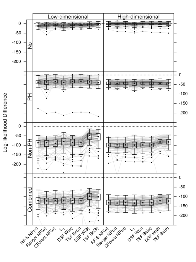
Figure 1: Prognostic data-generating process. Performance of competitors (random survival forest, RF-S; Ranger; conditional inference forests, CForest; $L_{1}$ survival forests; transformation survival forests, TSF; and distributional survival forests, DSF; see Table 1) assessed by the difference between the out-of-sample log-likelihood of the competitor and the log-likelihood of the true generating process. Larger values of the difference are preferable. Eight scenarios, i.e. low- and high- dimensional prognostic variables for absent (No), proportional hazards (PH), non-proportional hazards (Non-PH), or a combination of PH and Non-PH (Combined) effects with $100$ repetitions each were simulated. Values smaller than $-250$ are not shown.

The distribution of the out-of-sample log-likelihood differences $\ell(\hat{\text{\boldmath$\vartheta$}}_{N})-\ell(\xi,\alpha)$ are presented in Figure 1. In the absence of any effect (first row of Figure 1), roughly the same degree of overfitting was observed for all competitors except RF-S and $L_{1}$. The latter two procedures exhibited a more pronounced overfitting. In the presence of a sole proportional hazards effect (second row of Figure 1), all competitors showed roughly the same performance. Regardless of whether the classical log-rank scores (based on the non-parametric basis functions $\text{\boldmath$a$}_{\text{NP}}$) or scores obtained from (4) featuring log-linear (DSF) or Bernstein (TSF) basis functions were applied, the log-likelihood difference did not seem to be affected. The loss induced by a too rich parameterization ($\text{W}(\alpha)$ vs. $\text{W}(\text{\boldmath$\vartheta$})$ and $\text{Bs}(\alpha)$ vs. $\text{Bs}(\text{\boldmath$\vartheta$})$) was negligible. In the non-proportional hazard setting (third row of Figure 1), the distributional survival forest splitting in both the scale and shift parameters $\text{\boldmath$\vartheta$}=(\vartheta_{1},\vartheta_{2})^{\top}$ clearly outperformed all competitors except for the transformation survival forests that split in $\text{\boldmath$\vartheta$}\in\mathbb{R}^{6}$. As expected, $L_{1}$ forests were also able to pick-up this non-proportional signal, but to a lesser degree. All procedures employing log-rank splitting assuming proportional hazards performed similarly. The same conclusions could be drawn for the combined proportional and non-proportional effects setting, but the performance boost induced by the novel split criteria was less pronounced. The presence of $50$ variables in the high-dimensional setting only marginally affected the performance of all methods tested.

3.3 Predictive Models

We compared the performance of the novel transformation survival trees in the presence of a predictive effect to the performance of Weibull distributional survival trees (Seibold et al., 2018), i.e. the six predictive models from the first two columns of Table 1 were compared. The same parameter settings as described in Section 3.2 were applied. In addition, subsamples were stratified with respect to treatment assignment. We again compared the out-of-sample log-likelihood difference in the six scenarios (three effect types in low and high dimensions) for $100$ learning and validation samples of size $N=250$ and $\tilde{N}=500$, respectively (Figure 2).

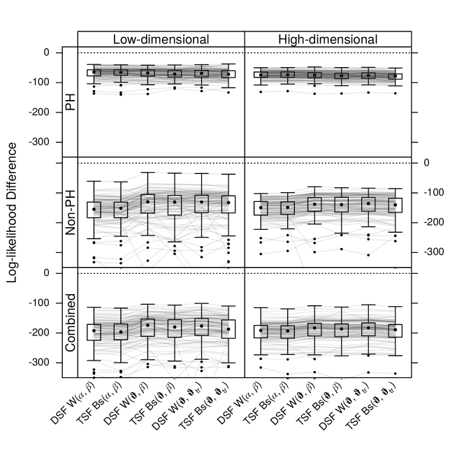
Figure 2: Predictive data-generating process. Performance of the predictive competitors distributional survival forests (DSF) and transformation survival forests (TSF) in the presence of a simulated predictive effect was measured as the difference between the out-of-sample log-likelihood of the competitor and the true generating process. Larger values of the difference are preferable. Six scenarios, i.e. low and high dimensions and proportional hazards (PH), non-proportional hazards (Non-PH) and a combination of PH and non-PH effects (Combined) with $100$ repetitions were simulated.

As expected, we found no differential performance in the proportional hazards setting (first row of Figure 2). Forests employing a split criterion sensitive to non-proportional effects performed better in the presence of a non-constant scale effect $\xi$ (second row of Figure 2). To a somewhat lesser extent, the same effect was observed when both proportional and non-proportional prognostic and predictive effects were simulated (third row of Figure 2). The impact of additional noise variables was only marginal.

4 Amyotrophic Lateral Sclerosis Survival

The Pooled Resource Open-Access ALS Clinical Trials (PRO-ACT, https://nctu.partners.org/ProACT) database contains longitudinal data of ALS patients who participated in one of $16$ phase II and III trials and one observational study. This project was initiated by the non-profit organization Prize4Life (http://www.prize4life.org/) to increase knowledge about ALS (Küffner et al., 2015). The database contains information on a broad variety of patient characteristics, such as vital signs, the patient’s and family’s history, and treatment information. Identification criteria, such as study centers, are not included in the database. From the PRO-ACT database, we generated a data set of $N=3306$ observations containing survival time and censoring information as well as baseline patient characteristics. Because not all procedures are able to deal with missing values in prognostic or predictive variables, a complete case analysis was performed. A more detailed description of the final data set of $N=2711$ observations and $18$ patient characteristics is available elsewhere (Seibold et al., 2018). To estimate the performance of the different procedures on the data set, we generated $100$ random splits of the data into learning and validation samples in a $3:1$ proportion, keeping the proportions of treated patients and the proportion of patients with right-censored overall survival time in all learning and validation samples the same as in the initial data set.

All survival forest variants discussed in this paper were applied using the same hyper-parameter settings as for the simulation study, including the use of bagging (i.e. no random variable selection). The number of randomly selected variables for splitting was set equal to the square root of the total number of variables. In addition to the out-of-sample log-likelihood of these competitors, the out-of-sample log-likelihoods of the following linear Weibull and Cox models is reported:

• Cox$()$: an unconditional Cox model that ignores patient characteristics,

• Weibull$(\alpha)$: A prognostic Weibull model with proportional hazard $\exp(\text{\boldmath$x$}^{\top}\text{\boldmath$\alpha$})$,

• Cox$(\alpha)$: a prognostic Cox model with proportional hazard $\exp(\text{\boldmath$x$}^{\top}\text{\boldmath$\alpha$})$,

• Weibull$(\alpha,\beta)$: a predictive Weibull model with proportional hazards
  $\exp(\text{\boldmath$x$}^{\top}\text{\boldmath$\alpha$}+\beta\mathds{1}\{r=1\}+\text{\boldmath$x$}^{\top}\text{\boldmath$\beta$}\mathds{1}\{r=1\}$), i.e. , including all treatment interactions,

• Cox$(\alpha,\beta)$: a predictive Cox model with proportional hazards
  $\exp(\text{\boldmath$x$}^{\top}\text{\boldmath$\alpha$}+\beta\mathds{1}\{r=1\}+\text{\boldmath$x$}^{\top}\text{\boldmath$\beta$}\mathds{1}\{r=1\}$),

where $\alpha$ denotes linear prognostic effects of $x$ and $\beta$ denotes linear differential predictive effects of $x$.

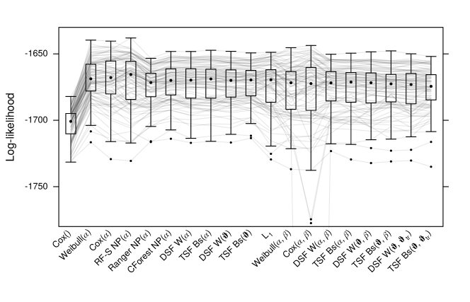
Figure 3: ALS survival. Out-of-sample log-likelihood estimation of prognostic and predictive models for $100$ random splits of ALS data into learning and validation samples with preserved treatment-censorship proportions. Larger values are preferable. One extreme value (for Cox$(\alpha,\beta)$) is not shown.

All methods taking patient characteristics into account outperformed the unconditional Cox model (Figure 3). We conclude that both prognostic and predictive models gain their superior performance by extracting information on patient’s survival time from the corresponding patient characteristics. Among the prognostic competitors, the linear Weibull and Cox models performed better than any of the survival forests except RF-S. Differences were, however, only marginal. This is a strong indication that neither non-linear interaction effects nor non-proportional hazard effects were necessary to capture the signal in the data. It is worth noting that different parameterizations of distributional and transformation survival forests performed highly similarly.

Predictive models did not noticeably better perform than prognostic models, which confirms that the treatment effect is very weak. Linear Weibull and Cox models that included treatment-covariate interactions performed as well as any of the distributional or transformation forests. Again, variants of the latter two procedures had only minor differences.

		Prognostic	Predictive
Variable	Category	$\exp(\text{\boldmath$\alpha$})$	$\exp(\text{\boldmath$\alpha$})$	$\exp(\beta),\exp(\text{\boldmath$\beta$})$
Treatment	Riluzole			1.39 (0.04, 43.58)
Time since onset		1.37 (1.28, 1.47)	1.24 (1.10, 1.39)	1.10 (0.95, 1.28)
Race	Asian	1.78 (0.56, 5.62)	1.52 (0.41, 5.61)	1.30 (0.13, 12.58)
	African A.	2.48 (1.02, 6.04)	3.10 (0.98, 9.83)	1.46 (0.12, 17.72)
	Unknown	0.77 (0.47, 1.26)	1.65 (0.70, 3.90)	0.27 (0.09, 0.79)
Sex	Male	0.89 (0.74, 1.07)	1.14 (0.86, 1.51)	0.72 (0.49, 1.05)
Age (in yrs)		0.96 (0.95, 0.96)	0.95 (0.94, 0.96)	1.00 (0.99, 1.02)
Height (in cm)		1.01 (1.00, 1.02)	1.01 (1.00, 1.03)	1.00 (0.98, 1.02)
Atrophy	Yes	0.79 (0.50, 1.25)	1.29 (0.59, 2.84)	0.57 (0.21, 1.56)
Cramps	Yes	0.52 (0.36, 0.75)	0.61 (0.33, 1.13)	0.81 (0.37, 1.75)
Fasciculations	Yes	1.09 (0.68, 1.75)	1.15 (0.54, 2.41)	1.11 (0.40, 3.06)
Gait changes	Yes	0.86 (0.45, 1.65)	4.23 (0.57, 31.25)	0.14 (0.02, 1.18)
Other changes	Yes	1.22 (0.70, 2.12)	1.47 (0.64, 3.41)	0.96 (0.29, 3.18)
Sensory changes	Yes	1.27 (0.65, 2.49)	0.92 (0.39, 2.16)	1.75 (0.46, 6.66)
Speech	Yes	0.73 (0.58, 0.90)	0.87 (0.61, 1.23)	0.72 (0.46, 1.14)
Stiffness	Yes	1.56 (0.77, 3.15)	2.11 (0.64, 6.94)	0.62 (0.14, 2.73)
Swallowing	Yes	0.97 (0.63, 1.51)	1.21 (0.54, 2.72)	0.97 (0.35, 2.67)
Weakness	Yes	0.69 (0.58, 0.82)	0.73 (0.53, 1.00)	0.90 (0.61, 1.33)
Family (Older)	Yes	1.05 (0.86, 1.27)	0.93 (0.69, 1.26)	1.12 (0.76, 1.65)
Family (Same)	Yes	0.93 (0.70, 1.23)	0.98 (0.63, 1.53)	0.90 (0.51, 1.60)
Family (Younger)	Yes	1.30 (0.64, 2.62)	1.31 (0.47, 3.69)	0.99 (0.24, 4.14)

Table 2: ALS survival. Estimated hazard ratios and corresponding unadjusted $95\%$ confidence intervals from prognostic and predictive linear Weibull models learned on the ALS data ($N=2711$ observations, $851$ of whom died). The reference category for treatment is placebo; that for race is Caucasian. Time since onset was measured in years, and family history was coded as three binary variables (older relatives affected by ALS, relatives in the same or younger generation).

The results of this model evaluation indicate that simple linear prognostic or predictive Weibull models can be used to adequately describe the impact of patient characteristics on the survival time. We estimated hazard ratios with unadjusted $95\%$ confidence intervals of prognostic and predictive Weibull models, based on the entire ALS data set of $N=2711$ complete cases (Table 2). In the prognostic model, seven variables strongly affected the outcome (time since onset, race, age, height, cramps, speech, and weakness). In the predictive model, only three prognostic variables (time since onset, age, weakness) in the presence of one predictive contrast (unknown race) affected the outcome. The permutation variable importance, using the log-likelihood of the corresponding trees as error function, of the prognostic distributional survival forest W$(\alpha)$ and the predictive distributional survival forests W$(\alpha,\beta)$ qualitatively coincided with the findings of the linear Weibull models, i.e. the variables time since onset, age, height, cramps, speech, and weakness were more important than the remaining variables in the prognostic model. The variables time since onset, age, and weakness showed up in the predictive distributional survival forest.

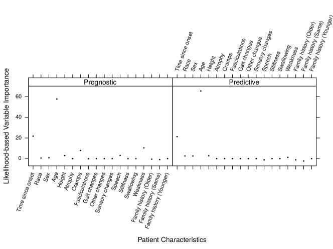
Figure 4: ALS survival. Likelihood-based permutation variable importance of prognostic (left) and predictive (right) distributional survival forests DSF W$(\alpha)$ and DFS W$(\alpha,\beta)$, respectively.

5 Discussion

The authors of the first regression tree method (Morgan and Sonquist, 1963), called automated interaction detection (AID), motivated the need for such a procedure to overcome the limitations of linearity and additivity in linear regression. In the same spirit, modern successors of AID are commonly understood as representatives of non-parametric regression methods. With the rise of statistical and machine learning, the superb accuracy of, for example, random forests (Breiman, 2001a) with its poor interpretability on the one hand, and the often poor accuracy but excellent interpretability of classical linear models on the other hand, motivated the dichotomous understanding of algorithmic versus parametric modelling cultures (Breiman, 2001b).

While assumptions like additivity and linearity could, in fact, be successfully overcome in the algorithmic modelling culture, other classical assumptions inherent in the parametric modelling culture did not likewise magically disappear. It was earlier demonstrated (Athey et al., 2018; Hothorn and Zeileis, 2017) that random forests rely on homogeneous residual variances and, consequently, quantile regression forests (Meinshausen, 2006) are unable to adapt to patterns where only the variance depends on certain explanatory variables. Here, we used a similar line of argumentation to demonstrate that survival forests, or at least prominent implementations that rely on trees based on log-rank split statistics for cut-point estimation, inherit the assumption of proportional hazards from the corresponding Cox model that defines the associated log-rank score statistics.

From a parametric modelling point of view, model-based transformation survival forests are fruitful in two ways. First, the underlying Cox models can be extended to allow time-varying effects. Thus, patterns emerging under non-proportional hazards can be described and, consequently, detected by appropriate score statistics in survival trees and forests. Second, it is possible to enrich simple prognostic models with treatment effects such that survival trees and forests for the identification of differential treatment effects can be developed for randomized clinical trial data.

From a practical point of view, our re-analysis of the PRO-ACT database of ALS patients demonstrated that neither non-linear, interaction, nor non-proportional hazards effects are necessary to describe prognostic and predictive models for ALS survival time. Simple linear Weibull models performed similarly to the most flexible transformation survival forests introduced here. Consequently, we gain simplicity of model interpretation without compromising model accuracy. Of course, this finding is mostly due to a low signal-to-noise ratio in this specific long-standing and difficult to address problem.

As a by-product, the novel distributional and transformation survival forests are able to deal with random left-censoring and interval-censoring as well as left-, right-, and interval truncation (the necessary changes to the likelihood and score functions are explained in Hothorn et al., 2018b, and are implemented in the trtf package, see next Section). Thus, survival forests featuring time-varying prognostic variables can be set up using these procedures. The survival forests discussed here extend currently proposed survival tree methods for interval-censored data (Fu and Simonoff, 2017; Drouin et al., 2017). The former method relies on score statistics from a Cox model and thus inherits specific power for detecting proportional-hazard-type signals. The latter maximum margin interval trees employ a specific Hinge loss adapted to the interval-censored case. The connection of this approach to proportional hazards models remains to be investigated. As an additional feature, the log-likelihood function associated with distributional and transformation survival forests allows permutation variable importance measures to be obtained also in the presence of random censoring and truncation, thus waiving the need for falling back on general scoring rules, such as the inverse probability of censoring-weighted Brier score (Graf et al., 1999).

A limitation of our study is the lack of attention paid to the impact caused by the implementation of different aggregation schemes. Because we were exclusively interested in a fair comparison of different split statistics, the same aggregation via local adaptive maximum-likelihood estimation was applied to all types of survival forests studied herein. However, RF-S, Ranger, and $L_{1}$ survival forests aggregate by averaging on the cumulative hazard scale whereas CForest computes nearest-neighbor weighted Kaplan-Meier curves. Future research shall focus on this additional and important difference that distinguishes the wide range of survival forests available to practitioners.

Computational Details

All computations were performed using R version 3.5.2 (R Core Team, 2018). The code for data preprocessing of the PRO-ACT data is available in the TH.data add-on package (Hothorn, 2019a). Patient-level data are available to registered users from https://nctu.partners.org/ProACT. Distributional and transformation survival forests were computed using the traforest() function from the trtf add-on package (Hothorn, 2019b). Random survival forests were obtained from the randomForestSRC add-on package (Ishwaran and Kogalur, 2019). The other two survival forests based on log-rank split statistics were CForest (function cforest() from the party add-on package, Hothorn et al., 2018a) and Ranger (package ranger, Wright et al., 2019). $L_{1}$ survival forests were computed with a privately patched version of randomForestsSRC provided to the authors by Professor Denis Laroque, HEC Montréal, Canada.

The trtf package was built on top of the infrastructure packages partykit (Hothorn and Zeileis, 2015) and mlt (Hothorn, 2018). For the empirical evaluation in Section 3, all survival forests except Ranger were fitted using the same $250$ subsamples of size $.632N$ (ranger version 0.11.1 does not allow subsamples to be specified ). Trees were restricted to at least $20$ observations in each terminal node and a maximal tree depth of $10$. None of the tree growing algorithms applied internal prepruning. For the low-dimensional simulations, bagging was applied. In all other settings and the analysis of the ALS data, a random subset of size $\sqrt{J}$ of the available prognostic or predictive variables was considered for splitting only (mtry parameter). For transformation survival forests, transformation functions were parameterized in terms of Bernstein polynomials for log-time of order five. Log-likelihoods were optimized under monotonicity constraints using a combination of augmented Lagrangian minimization and spectral projected gradients.

For the curious reader, we provide a small example of how the prognostic transformation survival forest TSF Bs$(\text{\boldmath$\vartheta$})$ and the predictive transformation survival forest TSF Bs($\text{\boldmath$\vartheta$},\beta)$ can be estimated for the publically available German Breast Cancer Study Group-2 data:

### attach data and packages
data("GBSG2", package = "TH.data")
library("survival") # CRAN: survival infrastructure
library("tram")     # CRAN: transformation models
library("trtf")     # CRAN: transformation trees and forests
set.seed(290875)    # make results reproducible

### prognostic model for GBSG2
## fit unconditional Cox model, with in-sample log-likelihood
logLik(m_prog <- Coxph(Surv(time, cens) ~ 1,
                       data = GBSG2, log_first = TRUE))

## ’log Lik.’ -2638.152 (df=7)

## fit TSF(theta)
TSF_prog <- traforest(m_prog, formula = Surv(time, cens) ~ .,
                      data = GBSG2)
## compute out-of-bag log-likelihood
logLik(TSF_prog, OOB = TRUE)

## ’log Lik.’ -2596.698 (df=NA)

### predictive model for GBSG2
## fit conditional Cox model with PH effect of hormonal treatment
logLik(m_pred <- Coxph(Surv(time, cens) ~ horTh,
                       data = GBSG2, log_first = TRUE))

## ’log Lik.’ -2633.649 (df=8)

## fit TSF(theta, beta)
TSF_pred <- traforest(m_pred,
                      formula = Surv(time, cens) | horTh ~ .,
                      data = GBSG2)
## compute out-of-bag log-likelihood
logLik(TSF_pred, OOB = TRUE)

## ’log Lik.’ -2601.604 (df=NA)

Corresponding predict() methods allow computation of conditional survivor or hazard functions as well as differential treatment effects $\beta(\text{\boldmath$x$})$ from the resulting models. Computing the distributional survival forests only requires that the Coxph() function be replaced with a call to Survreg(). The code necessary to reproduce the empirical results reported in this paper is available from within R

system.file("survival_forests", package = "trtf")

References

- Athey et al. (2018) Athey S, Tibshirani J, Wager S (2018). “Generalized Random Forests.” The Annals of Statistics. https://arxiv.org/pdf/1610.01271.pdf.
- Beaulieu-Jones et al. (2016) Beaulieu-Jones BK, Greene CS, the Pooled Resource Open-Access ALS Clinical Trials (2016). “Semi-supervised Learning of the Electronic Health Record for Phenotype Stratification.” Journal of Biomedical Informatics, 64, 168–178. 10.1016/j.jbi.2016.10.007.
- Breiman (2001a) Breiman L (2001a). “Random Forests.” Machine Learning, 45(1), 5–32. 10.1023/A:1010933404324.
- Breiman (2001b) Breiman L (2001b). “Statistical Modeling: The Two Cultures.” Statistical Science, 16(3), 199–231. 10.1214/ss/1009213726.
- Brooks et al. (1996) Brooks BR, Sanjak M, Ringel S, England J, Brinkmann J, Pestronk A, Florence J, Mitsumoto H, Szirony K, Wittes J (1996). “The Amyotrophic Lateral Sclerosis Functional Rating Scale: Assessment of Activities of Daily Living in Patients With Amyotrophic Lateral Sclerosis.” Archives of Neurology, 53(2), 141–147.
- Cedarbaum et al. (1999) Cedarbaum JM, Stambler N, Malta E, Fuller C, Hilt D, Thurmond B, Nakanishi A (1999). “The ALSFRS-R: A Revised ALS Functional Rating Scale That Incorporates Assessments of Respiratory Function.” Journal of the Neurological Sciences, 169(1), 13–21.
- Chiò et al. (2009) Chiò A, Logroscino G, Hardiman O, Swingler R, Mitchell D, Beghi E, Traynor BG on behalf of the Eurals Consortium (2009). “Prognostic Factors in ALS: A Critical Review.” Amyotrophic Lateral Sclerosis, 10(5-6), 310–323. 10.3109/17482960802566824.
- Datema et al. (2012) Datema FR, Moya A, Krause P, Bäck T, Willmes L, Langeveld T, de Jong RJB, Blom HM (2012). “Novel Head and Neck Cancer Survival Analysis Approach: Random Survival Forests versus Cox Proportional Hazards Regression.” Head & Neck, 34(1), 50–58. 10.1002/hed.21698.
- Drouin et al. (2017) Drouin A, Hocking TD, Laviolette F (2017). “Maximum Margin Interval Trees.” In I Guyon, UV Luxburg, S Bengio, H Wallach, R Fergus, S Vishwanathan, R Garnett (eds.), Advances in Neural Information Processing Systems 30, pp. 4947–4956. Curran Associates, Inc. URL http://papers.nips.cc/paper/7080-maximum-margin-interval-trees.pdf.
- Fang et al. (2018) Fang T, Khleifat AA, Meurgey JH, Jones A, Leigh PN, Bensimon G, Al-Chala A (2018). “Stage at Which Riluzole Treatment Prolongs Survival in Patients with Amyotrophic Lateral Sclerosis: A Retrospective Analysis of Data from a Dose-ranging Study.” Lancet Neurology, 17, 416–422. 10.1016/S1474-4422(18)30054-1.
- Friedman (1991) Friedman JH (1991). “Multivariate Adaptive Regression Splines.” The Annals of Statistics, 19(1), 1–67.
- Fu and Simonoff (2017) Fu W, Simonoff JS (2017). “Survival Trees for Interval-censored Survival Data.” Statistics in Medicine, 36(30), 4831–4842. 10.1002/sim.7450.
- Fujimura-Kiyono et al. (2011) Fujimura-Kiyono C, Kimura F, Ishida S, Nakajima H, Hosokawa T, Sugino M, Hanafusa T (2011). “Onset and Spreading Patterns of Lower Motor Neuron Involvements Predict Survival in Sporadic Amyotrophic Lateral Sclerosis.” Journal of Neurology, Neurosurgery & Psychiatry, 82(11), 1244–1249. 10.1136/jnnp-2011-300141.
- Graf et al. (1999) Graf E, Schmoor C, Sauerbrei W, Schumacher M (1999). “Assessment and Comparison of Prognostic Classification Schemes for Survival Data.” Statistics in Medicine, 18(17-18), 2529–2545. 10.1002/(SICI)1097-0258(19990915/30)18:17/18<2529::AID-SIM274>3.0.CO;2-5.
- Hothorn (2018) Hothorn T (2018). “Most Likely Transformations: The mlt Package.” Journal of Statistical Software. https://cran.r-project.org/web/packages/mlt.docreg/vignettes/mlt.pdf.
- Hothorn (2019a) Hothorn T (2019a). TH.data: TH’s Data Archive. R package version 1.0-10, URL http://CRAN.R-project.org/package=TH.data.
- Hothorn (2019b) Hothorn T (2019b). trtf: Transformation Trees and Forests. R package version 0.3-5, URL http://CRAN.R-project.org/package=trtf.
- Hothorn et al. (2018a) Hothorn T, Hornik K, Strobl C, Zeileis A (2018a). party: A Laboratory for Recursive Partytioning. R package version 1.3-1, URL http://party.R-forge.R-project.org.
- Hothorn and Jung (2014) Hothorn T, Jung HH (2014). “RandomForest4Life: A Random Forest for Predicting ALS Disease Progression.” Amyotrophic Lateral Sclerosis and Frontotemporal Degeneration, 15, 444–452. 10.3109/21678421.2014.893361.
- Hothorn et al. (2004) Hothorn T, Lausen B, Benner A, Radespiel-Tröger M (2004). “Bagging Survival Trees.” Statistics in Medicine, 23(1), 77–91. 10.1002/sim.1593.
- Hothorn et al. (2018b) Hothorn T, Möst L, Bühlmann P (2018b). “Most Likely Transformations.” Scandinavian Journal of Statistics, 45(1), 110–134. 10.1111/sjos.12291.
- Hothorn and Zeileis (2015) Hothorn T, Zeileis A (2015). “partykit: A Modular Toolkit for Recursive Partytioning in R.” Journal of Machine Learning Research, 16, 3905–3909. URL http://jmlr.org/papers/v16/hothorn15a.html.
- Hothorn and Zeileis (2017) Hothorn T, Zeileis A (2017). “Transformation Forests.” Technical report, arXiv 1701.02110, v2. URL https://arxiv.org/abs/1701.02110.
- Ishwaran and Kogalur (2019) Ishwaran H, Kogalur UB (2019). randomForestSRC: Random Forests for Survival, Regression, and Classification (RF-SRC). R package version 2.8.0, URL https://CRAN.R-project.org/package=randomForestSRC.
- Ishwaran et al. (2008) Ishwaran H, Kogalur UB, Blackstone EH, Lauer MS (2008). “Random Survival Forests.” The Annals of Applied Statistics, 2(3), 841–860. 10.1214/08-aoas169.
- Kimura et al. (2006) Kimura F, Fujimura C, Ishida S, Nakajima H, Furutama D, Uehara H, Shinoda K, Sugino M, Hanafusa T (2006). “Progression Rate of ALSFRS-R at Time of Diagnosis Predicts Survival Time in ALS.” Neurology, 66(2), 265–267. 10.1212/01.wnl.0000194316.91908.8a.
- Küffner et al. (2015) Küffner R, Zach N, Norel R, Hawe J, Schoenfeld D, Wang L, Li G, Fang L, Mackey L, Hardiman O, Cudkowicz M, Sherman A, Ertaylan G, Grosse-Wentrup M, Hothorn T, van Ligtenberg J, Macke JH, Meyer T, Schölkopf B, Tran L, Vaughan R, Stolovitzky G, Leitner ML (2015). “Crowdsourced Analysis of Clinical Trial Data to Predict Amyotrophic Lateral Sclerosis Progression.” Nature Biotechnology, 33, 51–57. 10.1038/nbt.3051.
- Lin and Jeon (2006) Lin Y, Jeon Y (2006). “Random Forests and Adaptive Nearest Neighbors.” Journal of the American Statistical Association, 101(474), 578–590. 10.1198/016214505000001230.
- Mandrioli et al. (2017) Mandrioli J, Rosi E, Fini N, Fasano A, Raggi S, Fantuzzi AL, Bedogni G (2017). “Changes in Routine Laboratory Tests and Survival in Amyotrophic Lateral Sclerosis.” Neurological Sciences, 38(12), 2177–2182. 10.1007/s10072-017-3138-8.
- McLain and Ghosh (2013) McLain AC, Ghosh SK (2013). “Efficient Sieve Maximum Likelihood Estimation of Time-Transformation Models.” Journal of Statistical Theory and Practice, 7(2), 285–303. 10.1080/15598608.2013.772835.
- Meinshausen (2006) Meinshausen N (2006). “Quantile Regression Forests.” Journal of Machine Learning Research, 7, 983–999. URL http://jmlr.org/papers/v7/meinshausen06a.html.
- Moradian et al. (2017) Moradian H, Larocque D, Bellavance F (2017). “ Splitting Rules in Survival Forests.” Lifetime Data Analysis, 23(4), 671–691. 10.1007/s10985-016-9372-1.
- Morgan and Sonquist (1963) Morgan JN, Sonquist JA (1963). “Problems in the Analysis of Survey Data, and a Proposal.” Journal of the American Statistical Association, 58, 415–434.
- Ong et al. (2017) Ong ML, Tan PF, Holbrook JD (2017). “Predicting Functional Decline and Survival in Amyotrophic Lateral Sclerosis.” PLoS ONE, 12(4), e0174925. 10.1371/journal.pone.0174925.
- Pfohl et al. (2018) Pfohl SR, Kim RB, Coan GS, Mitchell CS (2018). “Unraveling the Complexity of Amyotrophic Lateral Sclerosis Survival Prediction.” Frontiers in Neuroinformatics, 12, 12. 10.3389/fninf.2018.00036.
- R Core Team (2018) R Core Team (2018). R: A Language and Environment for Statistical Computing. R Foundation for Statistical Computing, Vienna, Austria. URL https://www.R-project.org/.
- Schlosser et al. (2018) Schlosser L, Hothorn T, Stauffer R, Zeileis A (2018). “Distributional Regression Forests for Probabilistic Precipitation Forecasting in Complex Terrain.” Technical report, arXiv 1804.02921, v2. URL https://arxiv.org/abs/1804.02921.
- Segal (1988) Segal MR (1988). “Regression Trees for Censored Data.” Biometrics, 44(1), 35–47. 10.2307/2531894.
- Seibold et al. (2016) Seibold H, Zeileis A, Hothorn T (2016). “Model-based Recursive Partitioning for Subgroup Analyses.” International Journal of Biostatistics, 12(1), 45–63. 10.1515/ijb-2015-0032.
- Seibold et al. (2018) Seibold H, Zeileis A, Hothorn T (2018). “Individual Treatment Effect Prediction for Amyotrophic Lateral Sclerosis Patients.” Statistical Methods in Medical Research, 27(10), 3104–3125. 10.1177/0962280217693034.
- Wright et al. (2017) Wright MN, Dankowski T, Ziegler A (2017). “Unbiased Split Variable Selection for Random Survival Forests using Maximally Selected Rank Statistics.” Statistics in Medicine, 36(8), 1272–1284. 10.1002/sim.7212.
- Wright et al. (2019) Wright MN, Wager S, Probst P (2019). ranger: A Fast Implementation of Random Forests. R package version 0.11.1, URL https://CRAN.R-project.org/package=ranger.
- Wright and Ziegler (2017) Wright MN, Ziegler A (2017). “ranger: A Fast Implementation of Random Forests for High Dimensional Data in C++ and R.” Journal of Statistical Software, 77(1). 10.18637/jss.v077.i01.
- Zoccolella et al. (2008) Zoccolella S, Beghi E, Palagano G, Fraddosio A, Guerra V, Samarelli V, Lepore V, Simone IL, Lamberti P, Serlenga L, Logroscino G for the SLAP Registry (2008). “Analysis of Survival and Prognostic Factors in Amyotrophic Lateral Sclerosis: A Population Based Study.” Journal of Neurology, Neurosurgery & Psychiatry, 79(1), 33–37. 10.1136/jnnp.2007.118018.