Higher symplectic capacities

Abstract.

We construct a new family of symplectic capacities indexed by certain symmetric polynomials, defined using rational symplectic field theory. We prove various structural properties of the capacities and discuss the connections with the equivariant $\mathcal{L}_{\infty}$ structure on symplectic cohomology and curve counts with tangency constraints. We also give some preliminary computations in basic examples and show that they give new state of the art symplectic embedding obstructions.

1. Introduction

1.1. Symplectic embeddings and symplectic capacities

Given a symplectic manifold $(M^{2n},\omega)$ and a function $H:M\rightarrow\mathbb{R}$, flowing along the symplectic gradient of $H$ defines a family of symplectomorphisms from $M$ to itself. Such Hamiltonian dynamical systems provide the geometric basis of classical mechanics and appear in various guises throughout mathematics and physics. It has been known since the 19th century that symplectomorphisms preserve the canonical volume form $\tfrac{1}{n!}\omega^{\wedge n}$, a result known as Liouville’s theorem in statistical mechanics. However, in his seminal 1985 paper [28] on pseudoholomorphic curves, Gromov showed that symplectomorphisms are much more subtle and mysterious than volume-preserving maps. The first proof of concept for this underlying richness is Gromov’s celebrated “nonsqueezing theorem”, which states that a large ball cannot be symplectically squeezed into a narrow infinite cylinder. More precisely, for $0<a^{\prime}<a$ there is no symplectic embedding

$$B^{2n}(a)\hookrightarrow B^{2}(a^{\prime})\times\mathbb{C}^{n-1}.$$

Here both sides are equipped with their canonical symplectic structures coming from the restriction of the standard symplectic form $\sum_{i=1}^{n}dx_{i}\wedge dy_{i}$ on $\mathbb{C}^{n}$, and $B^{2n}(a)$ denotes the ball of area $a$ (i.e. radius $\sqrt{a/\pi}$). Such an embedding is perfectly allowed by volume considerations alone, so this shows that symplectic geometry imposes fundamental and previously unanticipated constraints.

Understanding the precise nature of symplectic transformations is still a largely open field of research. After the nonsqueezing theorem, a natural next toy question is when can one symplectic ellipsoid be embedded into another. We define the symplectic ellipsoid $E(a_{1},...,a_{n})$ by

$$E(a_{1},...,a_{n}):=\left\{(z_{1},...,z_{n})\in\mathbb{C}^{n}\;:\;\sum_{k=1}^{n}\frac{\pi|z_{k}|^{2}}{a_{k}}\leq 1\right\}.$$

For convenience, we will always assume $a_{1}\leq...\leq a_{n}$. Note that we have special cases $E(a,...,a)=B^{2n}(a)$ and $E(a,\infty,...,\infty)=B^{2}(a)\times\mathbb{C}^{n-1}$.

Question 1.1.

For which $a_{1},...,a_{n}$ and $a_{1}^{\prime},...,a_{n}^{\prime}$ is there a symplectic embedding of $E(a_{1},...,a_{n})$ into $E(a_{1}^{\prime},...,a_{n}^{\prime})$?

Note that the volume of $E(a_{1},...,a_{n})$ is given by $\tfrac{1}{n!}a_{1}...a_{n}$, so the first basic obstruction is

$$a_{1}...a_{n}\leq a_{1}^{\prime}...a_{n}^{\prime}.$$

Also, Gromov’s nonsqueezing theorem can be rephrased as saying that there is no symplectic embedding

$$E(a,...,a)\hookrightarrow E(a^{\prime},\infty,...,\infty)$$

unless $a\leq a^{\prime}$, and this implies that in general we must have

$$a_{1}\leq a_{1}^{\prime}.$$

For $n=1$, an embedding evidently exists if and only if $a_{1}\leq a_{1}^{\prime}$. For $n=2$, the answer to Question 1.1 is now completely understood, or at least reduced to pure combinatorics. Before recalling the result, it is useful to formalize symplectic embedding obstructions using the notion of a symplectic capacity. Roughly, a symplectic capacity $\mathfrak{c}$ is any invariant of symplectic manifolds which takes values in positive real numbers and is monotone with respect to symplectic embeddings. More precisely, the symplectic capacities considered in this paper will only be defined for symplectic manifolds with nonempty convex boundary (although one could formally extend them to all symplectic manifolds if desired). We will also distinguish between “exact symplectic capacities”, which are monotone only for exact symplectic embeddings, and “non-exact symplectic capacities”, which are monotone for all symplectic embeddings. By default, “capacity” will mean exact, but we note that this distinction is immaterial if $H^{1}(-;\mathbb{R})=0$. One often also requires a symplectic capacity $\mathfrak{c}$ to scale like area, i.e. $\mathfrak{c}(M,a\omega)=a\mathfrak{c}(M,\omega)$, which rules out things like higher dimensional volume. This property will indeed hold for all the capacities discussed in this paper. Finally, some authors include the normalization condition $\mathfrak{c}(B^{2n})=\mathfrak{c}(B^{2}\times\mathbb{C}^{n-1})=1$. This property will not hold for most of the capacities considered in this paper.

An important sequence of symplectic capacities $\mathfrak{c}_{1}^{\operatorname{EH}},\mathfrak{c}_{2}^{\operatorname{EH}},\mathfrak{c}_{3}^{\operatorname{EH}},...$ were defined by Ekeland–Hofer in [14, 15] using variational methods. The first Ekeland–Hofer capacity satisfies

$$\mathfrak{c}_{1}^{\operatorname{EH}}(B^{2n}(r))=\mathfrak{c}_{1}^{\operatorname{EH}}(B^{2}(r)\times\mathbb{C}^{n-1})=r,$$

and so in particular recovers Gromov’s nonsqueezing theorem. More generally, for $k\in\mathbb{Z}_{>0}$, the $k$th Ekeland–Hofer capacity of the ellipsoid $E(a_{1},...,a_{n})$ has been computed to be the $k$th smallest element in the infinite matrix $(ia_{j}\;:\;i\in\mathbb{Z}_{>0},1\leq j\leq n)$. For example, the first few values for $E(1,2)$ are $1,2,2,3,4,4,5,...$ and the first few values for $E(1.5,1.5)$ are $1.5,1.5,3,3,4.5,4.5,6,...$, and hence $c_{2}^{\operatorname{EH}}$ rules out the existence of a symplectic embedding $E(1,2)\hookrightarrow E(1.5,1.5)$.

Although the Ekeland–Hofer capacities give nice embedding obstructions beyond Gromov’s nonsqueezing theorem, the four dimensional symplectic embedding problem is controlled by another sequence of symplectic capacities $\mathfrak{c}_{1}^{\operatorname{ECH}},\mathfrak{c}_{2}^{\operatorname{ECH}},\mathfrak{c}_{3}^{\operatorname{ECH}},...$ defined by Hutchings in [34] using embedded contact homology (ECH). Unlike the Ekeland–Hofer capacities, these capacities are gauge-theoretic in nature and are only defined in dimension four, but in that dimension they tend to give very strong obstructions. The $k$th ECH capacity of the ellipsoid $E(a,b)$ has been computed to be the $(k+1)$st smallest element in the infinite matrix $(ia+jb\;:\;i,j\in\mathbb{Z}_{\geq 0})$. For example, the first few values for $E(1,2)$ are $1,2,2,3,3,4,4,4,...$ and the first few values for $E(1.5,1.5)$ are $1.5,1.5,3,3,3,4.5,4.5,4.5,4.5,...$, etc. McDuff proved the following result in [45] (see the references therein for the history):

Theorem 1.2.

There is a symplectic embedding of $E(a,b)$ into $E(c,d)$ if and only if $\mathfrak{c}_{k}^{\operatorname{ECH}}(E(a,b))\leq\mathfrak{c}_{k}^{\operatorname{ECH}}(E(c,d))$ for all $k\in\mathbb{Z}_{>0}$.

Note that up to a scaling factor we can write $E(a,b)$ as $E(1,x)$ for some $x\geq 1$. In the special case $c=d$ (i.e. the target is a ball), the answer can be summarized in terms of a function $f:[1,\infty)\rightarrow[1,\infty)$, with $f(x)$ defined to be the infimal $c$ such that there exists a symplectic embedding $E(1,x)\hookrightarrow E(c,c)$. McDuff–Schlenk [47] gave an explicit characterization of the function $f(x)$, discovering the following rather subtle features:

• for $x<\tau^{4}$, $f(x)$ is piecewise linear, with values determined by ratios of Fibonacci numbers (here $\tau=\frac{1+\sqrt{5}}{2}$ the golden ratio)

• for $x>(\tfrac{17}{6})^{2}$, $f(x)=\sqrt{x}$ (i.e. embeddings in this regime are obstructed only by volume)

• for $\tau^{4}<x<(\frac{17}{6})^{2}$, $f(x)$ alternates between the above two behaviors.

In higher dimensions, Question 1.1 is still largely open. One surprising development was Guth’s construction [29] of symplectic embeddings

$$E(1,\underbrace{S,...,S}_{n-1})\hookrightarrow E(R,R,\underbrace{\infty,...,\infty}_{n-2})$$

for some finite $R$ and $S$ arbitrarily large. This shows that an infinite amount of squeezing is possible in the second factor, in significant contrast to the first factor. Hind and Kerman managed to refine Guth’s embedding and prove the following optimal result:

Theorem 1.3.

[31, 54] There exists a symplectic embedding

$$E(1,\underbrace{\infty,...,\infty}_{n-1})\hookrightarrow E(R,R,\underbrace{\infty,...,\infty}_{n-2})$$

if and only if $R\geq 3$.

More recent subsequent progress has focused on the following special case of Question 1.1:

Question 1.4 (“stabilized ellipsoid embedding problem”).

For which $a,b,c,d$ is there a symplectic embedding of $E(a,b,\underbrace{\infty,...,\infty}_{n-2})$ into $E(c,d,\underbrace{\infty,...,\infty}_{n-2})$?

Note that any symplectic embedding $E(a,b)\hookrightarrow E(c,d)$ can be stabilized to an embedding $E(a,b,\infty,...,\infty)\hookrightarrow E(c,d,\infty,...,\infty)$, but the converse need not hold. Indeed, the volume obstruction disappears after stabilizing, as do many of the ECH obstructions. For the special case $c=d$, i.e. embeddings of the form $E(1,x,\infty,...,\infty)\hookrightarrow E(c,c,\infty,...,\infty)$, notable progress has been made, the current state of the art being:

Theorem 1.5.

[31, 10, 11, 46] For $1\leq x\leq\tau^{4}$, the optimal $c$ is given by $f(x)$, i.e. the optimal embedding comes from the four dimensional case. For $x=\tfrac{3b_{n}}{b_{n}+1}$ with $b_{n}=\tfrac{g_{4n+6}}{g_{4n+2}}$ with $g_{i}$ the $i$th Fibonacci number (e.g. $b_{0}=8$, $b_{1}=55/8$, etc), or for $x=3d-1$ with $d\in\mathbb{Z}_{>0}$, the optimal $c$ is given by $\tfrac{3x}{x+1}$.

Although for $x>\tau^{4}$ the optimal embedding is not known, Hind has produced embeddings

$$E(1,x)\times\mathbb{C}^{n-2}\hookrightarrow E(\tfrac{3x}{x+1},\tfrac{3x}{x+1})\times\mathbb{C}^{n-2}$$

which are conjectured in [46] to be optimal. We mention that in all known cases the answer to Question 1.4 is independent of $n$ provided $n\geq 3$.

In this paper we primarily focus on the problem of obstructing high dimensional symplectic embeddings. The results comprising Theorem 1.5 have relied on the following basic strategy. First, given a four-dimensional symplectic embedding $E(1,x)\hookrightarrow E(c,c)$, one finds a rigid punctured pseudoholomorphic curve $C$ in the symplectic completion of the complementary cobordism $E(c,c)\setminus E(1,x)$ (see §3.1 for more on the geometric setup). The existence of such a curve is proved using embedded contact homology in [10], using obstruction bundle gluing in [46], and by neck-stretching closed curves in $\mathbb{CP}^{2}$ in [11]. One then argues that this curve meaningfully extends to the stabilization as a product curve $C\times\{pt\}$. Assuming this, a deformation argument shows that a similar curve $\widetilde{C}$ must also exist in the complementary cobordism of any hypothetical symplectic embedding $E(1,x,\infty,...,\infty)\hookrightarrow E(c,c,\infty,...,\infty)$. Finally, positivity of energy for $\widetilde{C}$ together with an application of Stokes’ theorem gives a lower bound for $c$ in terms of $x$.

The process of stabilizing the curve $C$ cannot always be achieved. Indeed, for an SFT-type curve $C$ with positive ends asymptotic to Reeb orbits $\gamma_{1}^{+},..,.,\gamma_{k}^{+}$ and negative ends asymptotic to Reeb orbits $\gamma^{-}_{1},...,\gamma^{-}_{l}$, the Fredholm index is given by

$${\operatorname{ind}}(C)=(n-3)(2-2g-k-l)+\sum_{i=1}^{k}{{\operatorname{CZ}}}(\gamma_{i}^{+})-\sum_{j=1}^{l}{{\operatorname{CZ}}}(\gamma_{j}^{-})+2c_{1}\cdot[C]$$

(see §3.2 for more details). Since stabilizing has the effect of increasing $n$ by $1$ and also increasing each Conley–Zehnder index ${{\operatorname{CZ}}}(\gamma)$ by $1$, the index after stabilizing is

$$2-2g-2l+{\operatorname{ind}}(C).$$

This means that $C\times\{pt\}$ will typically not be rigid, and might potentially even have negative index, in which case it ought to disappear after a small perturbation. However, a basic observation from [31] is that for genus zero curves with exactly one negative end, the index is unchanged by stabilization, and in fact such curves do generally persist to give higher dimensional obstructions. One of the main motivations of this paper is to understand whether these obstructions can be understood more systematically in terms of symplectic capacities which are defined in any dimension.

Remark 1.6.

One can of course also extend Question 1.1 to say more general star-shaped domains in $\mathbb{C}^{n}$, or to symplectic manifolds with more complicated topology. Ellipsoids are among the simplest symplectic domains from a dynamical point of view.

1.2. Capacities from Floer theory

Since Floer homology interacts favorably with the symplectic action functional, it is natural to try to use it to define symplectic capacities. Suppose that $X^{2n}$ is a Liouville domain, i.e. a compact symplectic manifold with boundary, whose symplectic form $\omega$ admits a global primitive $\lambda$ restricting to a positive contact form on $\partial X$. We associate to $X$ its symplectic cohomology ${\operatorname{SH}}(X)$, defined over say $\mathbb{K}=\mathbb{Q}$. We can also consider the underlying cochain complex ${\operatorname{SC}}(X)$, with its natural increasing action filtration

$$\mathcal{F}_{\leq a}{\operatorname{SC}}(X)\subset\mathcal{F}_{\leq a^{\prime}}{\operatorname{SC}}(X),\;\;\;\;\;0\leq a<a^{\prime},$$

with $\bigcup\limits_{a\in\mathbb{R}_{\geq 0}}\mathcal{F}_{\leq a}{\operatorname{SC}}(X)={\operatorname{SC}}(X)$. Roughly, ${\operatorname{SC}}(X)$ is generated as a $\mathbb{K}$-module by one generator for each critical point of a chosen Morse function on $X$, and two generators $\hat{\gamma},\check{\gamma}$ for each Reeb orbit $\gamma$ of $\partial X$, with differential $\partial$ counting Floer cylinders. The Morse complex of $X$ (defined over $\mathbb{K}$) sits inside ${\operatorname{SC}}(X)$ as the subcomplex of action zero elements:

$$C(M)=\mathcal{F}_{\leq 0}{\operatorname{SC}}(X)\subset{\operatorname{SC}}(X).$$

In particular, there is a canonical action zero element $e\in\mathcal{F}_{\leq 0}{\operatorname{SC}}(X)$ represented by the minimum of the Morse function, which we will refer to as the unit (even when not discussing product structures). Given any exact symplectic embedding $X\hookrightarrow X^{\prime}$, we have a filtration-preserving transfer map $\Phi:{\operatorname{SC}}(X^{\prime})\rightarrow{\operatorname{SC}}(X)$ sending unit to unit.

We define a symplectic capacity from this data as follows:

$$\mathfrak{c}(X):=\inf\{a\;:\partial(x)=e\text{ for some }x\in\mathcal{F}_{\leq a}{\operatorname{SC}}(X)\}.$$

It follows from standard invariance properties that $\mathfrak{c}(X)\in\mathbb{R}_{>0}$ is a symplectomorphism invariant of $X$, independent of any choices made during its construction (e.g. almost complex structures, Hamiltonians, etc). Moreover, given an exact symplectic embedding $X\hookrightarrow X^{\prime}$, we have the monotonicity property $\mathfrak{c}(X)\leq\mathfrak{c}(X^{\prime})$. Indeed, this follows from a simple diagram chase, since $x\in\mathcal{F}_{\leq a}{\operatorname{SC}}(X^{\prime})$ with $\partial x=e$ implies

$$\partial(\Phi x)=\Phi(\partial x)=\Phi(e)=e,$$

with $\Phi(x)\in\mathcal{F}_{\leq a}{\operatorname{SC}}(X)$.

Remark 1.7.

Although we work with increasing filtrations in this introduction for clarity of exposition, in the body of the paper we will instead work over a suitable Novikov ring $\Lambda_{\geq 0}$ and work with decreasing filtrations. For Liouville domains this perspective leads to an equivalent definition of the capacity $\mathfrak{c}$, but it has the advantage of making sense for more general symplectic manifolds with convex boundary and is defined without referencing any choice of primitive one-form. It will be also more natural when discussing Maurer–Cartan theory.

It is not hard to check that we have $\mathfrak{c}(B^{2n}(r))=r$ and $\mathfrak{c}(B^{2}(R)\times\mathbb{C}^{n})=R$, and hence the capacity $\mathfrak{c}$ recovers Gromov’s nonsqueezing theorem. However, in order to capture more refined obstructions we need more capacities. Recently, Gutt–Hutchings [30] have shown that by replacing symplectic cohomology with its $S^{1}$-equivariant analogue, we can extend $\mathfrak{c}(X)$ to a sequence of capacities $\mathfrak{c}_{1}^{{\operatorname{GH}}}(X),\mathfrak{c}_{2}^{{\operatorname{GH}}}(X),\mathfrak{c}_{3}^{{\operatorname{GH}}},...$ which conjecturally agree with the Ekeland–Hofer capacities. To explain the construction, recall that ${\operatorname{SC}}(X)$ naturally has the structure of an $S^{1}$-complex, which means we have a sequence of operations $\Delta_{i}:{\operatorname{SC}}(X)\rightarrow{\operatorname{SC}}(X)$ (of degree $1-2i$ when $\mathbb{Z}$ gradings are available), with $\Delta_{0}=\partial$, satisfying the relations

$$\sum_{i+j=k}\Delta_{i}\circ\Delta_{j}=0$$

for all $k\in\mathbb{Z}_{\geq 0}$. Here $\Delta_{1}$ descends to the BV operator on ${\operatorname{SH}}(X)$, while $\Delta_{k\geq 2}$ is a “higher BV operator” compensating for the failure of $\Delta_{1}$ to satisfy $\Delta_{1}^{2}=0$ on the nose. This structure has made various appearances in the literature, c.f. [57, 5] (see also [23] for a particularly succinct construction in terms of Floer cylinders with extra marked points). Let $\mathbb{K}[u^{-1}]$ be a shorthand for the $\mathbb{K}[u]$-module $\mathbb{K}[u,u^{-1}]/\left(u\mathbb{K}[u]\right)$. We define $S^{1}$-equivariant symplectic cochains ${\operatorname{SC}}_{S^{1}}$ by

$${\operatorname{SC}}_{S^{1}}(X):={\operatorname{SC}}(X)\otimes_{\mathbb{K}[u]}\mathbb{K}[u^{-1}],$$

with differential $\partial_{S^{1}}$ given by

$$\partial_{S^{1}}(x)=\sum_{i=0}^{\infty}\Delta_{i}(x)u^{i}$$

for $x\in{\operatorname{SC}}_{S^{1}}(X)$.

Remark 1.8.

There are two common variations on this definition of the $S^{1}$-equivariant complex: the negative version, in which one works over $\mathbb{K}\llbracket u\rrbracket$, and the periodic version, in which one works over $\mathbb{K}\llbracket u\rrbracket[u^{-1}]$. The version we use above is akin to taking homotopy orbits of an $S^{1}$-action.

There is a natural increasing action filtration on ${\operatorname{SC}}_{S^{1}}(X)$, and we have canonical elements $u^{-k}e\in\mathcal{F}_{\leq 0}{\operatorname{SC}}_{S^{1}}(X)\subset{\operatorname{SC}}_{S^{1}}(X)$ for $k\in\mathbb{Z}_{\geq 0}$. We define $\mathfrak{c}_{k}^{{\operatorname{GH}}}(X)\in\mathbb{R}_{>0}$ by

$$\mathfrak{c}_{k}^{{\operatorname{GH}}}(X):=\inf\{a\;:\;\partial(x)=u^{-k+1}e\text{ for some }x\in\mathcal{F}_{\leq a}{\operatorname{SC}}_{S^{1}}(X)\}.$$

Similar to before, exact symplectic embeddings $X\hookrightarrow X^{\prime}$ induce transfer maps ${\operatorname{SC}}_{S^{1}}(X^{\prime})\rightarrow{\operatorname{SC}}_{S^{1}}(X)$, from which it follows that $\mathfrak{c}_{k}^{{\operatorname{GH}}}(X)\leq\mathfrak{c}_{k}^{{\operatorname{GH}}}(X^{\prime})$.

To understand why the equivariant theory offers more quantitative data, we can rephrase the construction as follows. By quotienting out the Morse complex of $X$, we obtain a homology-level long exact sequence

$$...\rightarrow H(X)\rightarrow SH(X)\rightarrow SH_{+}(X)\rightarrow H(X)\rightarrow...,$$

where the last map is the connecting homomorphism $\delta:SH_{+}(X)\rightarrow H(X)$. We have the following equivalent homology level description:

$$\mathfrak{c}(X)=\inf\{a\;:\;\delta(x)=[e]\text{ for some }x\in\mathcal{F}_{\leq a}SH_{+}(X)\}.$$

In fact, we can define more general “spectral capacities” by replacing $[e]=1\in H^{0}(X)$ by any class in $H^{*}(X)$. However, if $X$ is say an ellipsoid or a more general a star-shaped domain in $\mathbb{C}^{n}$, we have ${\operatorname{SH}}_{+}(X)\cong H(X)\cong\mathbb{K}$, so there is essentially only one spectral invariant. In constrast, in the $S^{1}$-equivariant version we replace $H(X)$ by $H_{S^{1}}(X)\cong H(X)\otimes H(\mathbb{CP}^{\infty})$, giving rise to countably many independent classes even when $X$ is contractible.

Remark 1.9.

The capacities $\mathfrak{c}_{k}^{{\operatorname{GH}}}$ are certainly not monotone for non-exact symplectic embeddings, as can be easily seen from examples such as the annulus $D^{*}S^{1}$ in the two-ball $B^{2}$.

Assuming the Gutt–Hutchings capacities coincide with the Ekeland–Hofer capacities, this new definition via Floer theory still has a few advantages. Firstly, the basic structure of the capacities becomes more transparent. For instance, one immediately has the “Reeb orbit axiom” stating that $\mathfrak{c}_{k}^{{\operatorname{GH}}}(X)$ must be represented by the action of some Reeb orbit of $\partial X$, in a uniquely determined degree. Since irrational ellipsoids have a unique Reeb orbit in each allowed degree, this immediately determines $\mathfrak{c}_{k}^{{\operatorname{GH}}}$ for all ellipsoids. Using this together with the other basic properties, the authors in [30] manage to compute $\mathfrak{c}_{k}^{{\operatorname{GH}}}$ for all “convex toric domains” and “concave toric domains” (see loc. cit. for precise definitions). We also have the stability property $\mathfrak{c}_{k}^{{\operatorname{GH}}}(X\times\mathbb{C})=\mathfrak{c}_{k}^{{\operatorname{GH}}}(X)$, which follows from the Künneth theorem for symplectic cochains as an $S^{1}$-complex.

Secondly, and this is one of the main themes of this paper, we can try to further generalize these capacities by appealing to higher algebra structures sitting on top of symplectic cochains. Indeed, symplectic cohomology has (at least in characteristic zero) the structure of a BV-algebra. This means that there is a BV operator of degree $-1$, a supercommutative product of degree $0$, and a bracket of degree $-1$, satisfying certain compatibility conditions. Recall that both the product and the bracket are defined by counting Floer-theoretic pairs of pants, but with asymptotic markers treated differently. Also, the first two pieces of data determine the third in the sense that the bracket measures the failure of the BV operator to be a derivation.

So, a first idea might be to try to generalize the definition of $\mathfrak{c}_{1}^{{\operatorname{GH}}}$ by incorporating the product. Unfortunately, at least for $X$ a star-shaped domain, we have ${\operatorname{SH}}(X)=0$, so the product ${\operatorname{SH}}(X)\otimes{\operatorname{SH}}(X)\rightarrow{\operatorname{SH}}(X)$ contains no information, nor does it descend to a product ${\operatorname{SH}}_{+}(X)\otimes{\operatorname{SH}}_{+}(X)\rightarrow{\operatorname{SH}}_{+}(X)$. Therefore it is not immediately clear how to incorporate the product in the definition of spectral invariants, and the bracket suffers from similar deficiencies.

On the other hand, the product on symplectic cohomology actually comes from a chain level $\mathcal{A}_{\infty}$ structure, while the bracket comes from a chain level $\mathcal{L}_{\infty}$ structure. Recall that the structure of an $\mathcal{A}_{\infty}$ algebra consists of a sequence of $k$-to-$1$ operations satisfying a sequence of quadratic structure equations and giving rise to a homology-level associative algebra. $\mathcal{L}_{\infty}$ algebras are the natural Lie algebra analogues. In the case of symplectic cochains, the $\mathcal{A}_{\infty}$ operations $\mu^{k}$ have degree $2-k$, while the $\mathcal{L}_{\infty}$ operations $\ell^{k}$ have degree $3-2k$. In general, the data of an $\mathcal{L}_{\infty}$ algebra $V$ with structure maps $\ell^{1},\ell^{2},\ell^{3},...$ can be encoded into a single chain complex $\mathcal{B}V$, the bar complex, with differential $\widehat{\ell}:\mathcal{B}V\rightarrow\mathcal{B}V$ combining all the $\ell^{k}$ operations (there is a similar construction for $\mathcal{A}_{\infty}$ algebras). Here as a $\mathbb{K}$-module $\mathcal{B}V$ is simply the (reduced) symmetric tensor algebra $\overline{S}V$ of $V$. In particular, we think of $\overline{S}V$ as linear combinations of symmetric words (of length at least one) in $V$, and we denote by $\overline{S}_{\leq l}V$ the subcomplex consisting of words of length at most $l$.

There is also an $\mathcal{L}_{\infty}$ structure on the $S^{1}$-equivariant complex ${\operatorname{SC}}_{S^{1}}$, which is more directly relevant for extending the capacities $\mathfrak{c}_{k}^{{\operatorname{GH}}}(X)$ above. This underlies a Lie bracket on ${\operatorname{SH}}_{S^{1}}$, identified with the string bracket in the context of string topology (i.e. the case $X=T^{*}Q$). We denote by $\ell^{k}_{S^{1}}$ the $S^{1}$-equivariant $\mathcal{L}_{\infty}$ structure maps.

We now cook up a family of symplectic capacities based on the $\mathcal{L}_{\infty}$ algebra ${\operatorname{SC}}_{S^{1}}$ as follows. The bar complex $\mathcal{B}{\operatorname{SC}}_{S^{1}}(X)$ inherits an increasing action filtration, and words in the elements $u^{-k}e$, $k\in\mathbb{Z}_{\geq 0}$, generate a subcomplex of $\mathcal{F}_{\leq 0}\overline{S}{\operatorname{SC}}_{S^{1}}(X)\subset\mathcal{B}{\operatorname{SC}}_{S^{1}}(X)$ with trivial differential, which we identify with $\overline{S}\mathbb{K}[u^{-1}]$. Pick an element $\mathfrak{b}\in\overline{S}\mathbb{K}[u^{-1}]$. We define a symplectic capacity $\mathfrak{d}_{\mathfrak{b}}$ by

$$\mathfrak{d}_{\mathfrak{b}}(X):=\inf\{a\;:\;\mathfrak{b}=\widehat{\ell}_{S^{1}}(x)\text{ for some }x\in\mathcal{F}_{\leq a}\mathcal{B}{\operatorname{SC}}_{S^{1}}(X)\}.$$

As with $\mathfrak{c}_{k}^{{\operatorname{GH}}}(X)$ above, it follows from the invariance properties of symplectic cochains that $\mathfrak{d}_{\mathfrak{b}}(X)$ is a symplectomorphism invariant, independent of all choices involved in its construction, and is monotone with respect to exact symplectic embeddings.

Remark 1.10.

If $X$ is a star-shaped domain in $\mathbb{C}^{n}$, we have ${\operatorname{SH}}_{S^{1}}(X)=0$, and the homology of the bar complex $\mathcal{B}{\operatorname{SC}}_{S^{1}}(X)$ is also trivial. We can split off the elements of action zero, i.e. $\mathcal{F}_{\leq 0}\mathcal{B}{\operatorname{SC}}_{S^{1}}(X)$, which we identify with $\overline{S}\mathbb{K}[u^{-1}]$. Let $\mathcal{F}_{+}\mathcal{B}{\operatorname{SC}}_{S^{1}}(X)$ denote the quotient $\mathcal{B}{\operatorname{SC}}_{S^{1}}(X)/\mathcal{F}_{\leq 0}\mathcal{B}{\operatorname{SC}}_{S^{1}}(X)$. Then we have a homology-level connecting homomorphism

$$H(\mathcal{F}_{+}\mathcal{B}{\operatorname{SC}}_{S^{1}}(X))\rightarrow\overline{S}\mathbb{K}[u^{-1}],$$

which is in fact an isomorphism since $\mathcal{B}{\operatorname{SC}}_{S^{1}}(X)$ is acyclic. Under this identification, $\mathfrak{d}_{\mathfrak{b}}(X)$ is the minimal action of a homology class which maps to $\mathfrak{b}$. In essence, the capacities $\mathfrak{d}_{\mathfrak{b}}$ give the set of all spectral capacities associated to the bar complex $\mathcal{B}{\operatorname{SC}}_{S^{1},+}$, with homology classes canonically labeled by elements $\mathfrak{b}\in\overline{S}\mathbb{K}[t]$.

Since the bar complex $\mathcal{B}{\operatorname{SC}}_{S^{1}}(X)$ has another increasing filtration by word length, i.e. $\mathcal{B}_{\leq l}{\operatorname{SC}}_{S^{1}}(X)\subset\mathcal{B}_{\leq l^{\prime}}{\operatorname{SC}}_{S^{1}}(X)$ for $1\leq l<l^{\prime}$, we can refine the construction and define capacities $\mathfrak{d}_{\mathfrak{b}}^{\leq l}$ by

$$\mathfrak{d}_{\mathfrak{b}}^{\leq l}(X):=\inf\{a\;:\;\mathfrak{b}=\widehat{\ell_{S^{1}}}(x)\text{ for some }x\in\mathcal{F}_{\leq a}\mathcal{B}_{\leq l}{\operatorname{SC}}_{S^{1}}(X)\}.$$

Observe that in the special case with $l=1$ and $\mathfrak{b}=u^{-k+1}\in\overline{S}_{\leq 1}\mathbb{K}[u^{-1}]\subset\overline{S}\mathbb{K}[u^{-1}]$, $\mathfrak{d}_{u^{-k+1}}^{\leq 1}$ reduces to $\mathfrak{c}_{k}^{{\operatorname{GH}}}$, so the family of capacities $\mathfrak{d}_{\mathfrak{b}}^{\leq l}$ extends the Gutt–Hutchings capacities and conjecturally also the Ekeland–Hofer capacities.

1.3. Capacities from rational symplectic field theory

In this paper, our primary object of study is actually another family of symplectic capacities $\mathfrak{g}_{\mathfrak{b}}$, which we define via rational symplectic field theory (RSFT). Recall that while Floer theory involves counts of punctured pseuoholomorphic curves which are contained in compact subsets of the target symplectic manifold, the curves in symplectic field theory are proper and hence unbounded near each puncture (the relevant background is reviewed in §3). Note that in both theories we study a compact symplectic manifold $X$ by passing to its symplectic completion $\widehat{X}$. We conjecture these capacities $\mathfrak{g}_{\mathfrak{b}}$ to be equivalent to the capacities $\mathfrak{d}_{\mathfrak{b}}$ above (some evidence is provided in Remark 5.7). Such an equivalence notwithstanding, the advantage of the SFT approach is that the geometric and structural properties of the capacities are more transparent. In particular we use these properties to compute them in interesting examples and demonstrate their effectiveness beyond previously known capacities.

Disclaimer 1.11.

The invariants defined in this paper are based on rational symplectic field theory. We will assume that a general construction of rational symplectic field theory exists with the basic structure and invariance properties outlined in [18]. It is well-known that a fully rigorous such construction requires working in some sort of virtual perturbation framework for pseudoholomorphic curves. Such a framework is widely expected to exist and several proposals have been given, although consensus has not yet been reached regarding the status of these projects. We will not make use of any particularities of the virtual framework. See §3.4 below for a more detailed discussion.

Proceeding with the discussion of the capacities $\mathfrak{g}_{\mathfrak{b}}$, recall that positive symplectic cochains ${\operatorname{SC}}_{+}(X)$ has an equivalent model defined in terms of SFT, which we denote by ${\operatorname{CH}}_{{{\operatorname{lin}}},{\operatorname{non-eq}}}(X)$ (see [5] for details). As a $\mathbb{K}$-module it has two generators $\hat{\gamma},\check{\gamma}$ for each “good” Reeb orbit of $\partial X$. The differential between two orbits of the same decoration is the usual linearized contact homology differential counting anchored cylinders, while the differential from a check to hat generator counts cylinders with constrained asymptotic markers and also certain types of cascades. As explained by Bourgeois–Oancea in [5], we can also extend ${\operatorname{CH}}_{{{\operatorname{lin}}},{\operatorname{non-eq}}}(X)$ to the critical points of a chosen Morse function on $X$ to get ${\operatorname{CH}}_{{{\operatorname{lin}}},{\operatorname{non-eq}},{\operatorname{filled}}}(X)$, a model for ${\operatorname{SC}}(X)$. The complex ${\operatorname{CH}}_{{{\operatorname{lin}}},{\operatorname{non-eq}},{\operatorname{filled}}}(X)$ is by definition the mapping cone of a chain map $\epsilon:{\operatorname{CH}}_{{{\operatorname{lin}}},{\operatorname{non-eq}}}(X)\rightarrow C(M)$. The chain map $\epsilon$ vanishes on hat generators, while on check generators it counts pseudoholomorphic planes in $X$ attached to a gradient flowline from an interior marked point to a Morse critical point in $X$. In particular, the coefficient of $e$ is given by counting planes in $X$ with a marked point passing through the minimum, which we can think of as a chosen generic point $p_{e}\in X$. We can therefore informally interpret $\mathfrak{g}(X)$ as the minimal energy of a rigid pseudoholomorphic plane in $X$ passing through $p_{e}$, but with the following caveats:

• The asymptotic orbit $\gamma$ must be closed with respect to the linearized contact homology differential (but note that for an irrational ellipsoid this is automatic for degree parity reasons).

• We also allow $\gamma$ could be a $\mathbb{K}$-linear combination of (good) Reeb orbits.

• The algebraic count of such planes must be nonzero, and in general this count could be virtual.

Regarding the equivariant version, the SFT model for ${\operatorname{SC}}_{S^{1},+}(X)$ is given simply by linearized contact homology ${\operatorname{CH}}_{{\operatorname{lin}}}(X)$. However, extending this model to the constant orbits is somewhat more subtle. A model for ${\operatorname{CH}}_{{{\operatorname{lin}}},{\operatorname{filled}}}(X)$ is given in [5] but it does not have the correct properties. One algebraic way of defining an SFT model for ${\operatorname{SC}}_{S^{1}}(X)$ would be to start with the BV operator on ${\operatorname{CH}}_{{{\operatorname{lin}}},{\operatorname{non-eq}}}$, which as explained in [5] simply sends $\check{\gamma}$ to $\hat{\gamma}$ times its covering multiplicity, and then to pass to the algebraic quotient (as we did for ${\operatorname{SC}}_{S^{1}}$). Instead, we will take a different route as follows. We construct for each $m\geq 0$ a (shifted) augmentation $\epsilon_{{\operatorname{lin}}}\Langle\mathcal{T}^{m}p\Rangle:{\operatorname{CH}}_{{\operatorname{lin}}}(X)\rightarrow\mathbb{K}$ which is defined by counting curves in $X$ satisfying an order $m$ tangency constraint to a generic local divisor at a chosen point (this amounts to a real codimension $2m+2-2n$ constraint). Alternatively, as we explain in §5, we can define $\epsilon_{{\operatorname{lin}}}\Langle\mathcal{T}^{m}p\Rangle$ in terms of the structure coefficients of a certain RSFT cobordism map. Moreover, $\epsilon_{{\operatorname{lin}}}\Langle\mathcal{T}^{m}p\Rangle$ is not just a chain map but an $\mathcal{L}_{\infty}$ homomorphism from ${\operatorname{CH}}_{{\operatorname{lin}}}(X)$ to $\mathbb{K}$. Here the $\mathcal{L}_{\infty}$ structure $\ell_{1},\ell_{2},\ell_{3},...$ on ${\operatorname{CH}}_{{\operatorname{lin}}}(X)$ has a rather straightforward definition by counting rational curves in $\mathbb{R}\times\partial X$ with several positive ends and one negative end, plus additional anchors in $X$ (a related $\mathcal{L}_{\infty}$ augmentation plays a prominent role in [60]). These augmentations can be assembled into a single $\mathcal{L}_{\infty}$ homomorphism

$$\epsilon_{{\operatorname{lin}}}\Langle\mathcal{T}^{\bullet}p\Rangle:{\operatorname{CH}}_{{\operatorname{lin}}}(X)\rightarrow\mathbb{K}[t],$$

where $\mathbb{K}[t]$ is equipped with trivial $\mathcal{L}_{\infty}$ operations and the component corresponding to $t^{k}$ is given precisely by $\Langle\mathcal{T}^{k}p\Rangle$. We denote the induced map on bar complexes by

$$\widehat{\epsilon_{{\operatorname{lin}}}}\Langle\mathcal{T}^{\bullet}p\Rangle:\mathcal{B}{\operatorname{CH}}_{{\operatorname{lin}}}(X)\rightarrow\overline{S}\mathbb{K}[t].$$

For a chosen element $\mathfrak{b}\in\overline{S}\mathbb{K}[t]$, we define the symplectic capacity $g_{\mathfrak{b}}^{\leq l}$ by

$$\mathfrak{g}_{\mathfrak{b}}^{\leq l}(X):=\inf\{a\;:\;\mathfrak{b}=\widehat{\epsilon_{{\operatorname{lin}}}}\Langle\mathcal{T}^{\bullet}p\Rangle(x)\text{ for some }x\in\mathcal{F}_{\leq a}\mathcal{B}_{\leq l}{\operatorname{CH}}_{{\operatorname{lin}}}(X)\text{ with }\widehat{\ell}(x)=0\}.$$

It will also be convenient to define simplified capacities by

$$\mathfrak{g}^{\leq l}\Langle\mathcal{T}^{k}p\Rangle(X):=\inf_{\mathfrak{b}\;:\;\pi_{1}(\mathfrak{b})=t^{k}}\mathfrak{g}_{\mathfrak{b}}^{\leq l}(X),$$

where the infimum is over all $\mathfrak{b}\in\overline{S}\mathbb{K}[t]$ mapping to $t^{k}$ under the projection $\pi_{1}:\overline{S}\mathbb{K}[t]\rightarrow\overline{S}_{\leq 1}\mathbb{K}[t]=\mathbb{K}[t]$. Informally, $\mathfrak{g}^{\leq l}\Langle\mathcal{T}^{k}p\Rangle(X)$ is the minimal energy of a rigid connected rational curve with at most $l$ positive ends in $X$ which passes through the point $p_{e}$ and satisfies an order $k$ tangency constraint, subject to similar caveats as above. Similarly, for $\mathfrak{b}$ of the form $t^{k_{1}}\odot...\odot t^{k_{r}}$, $\mathfrak{g}_{\mathfrak{b}}^{\leq l}(X)$ is informally the minimal energy of a rigid rational curve in $X$ with $r$ components and at most $l$ positive ends, with the $i$th component passing through $p_{e}$ and satisfying an order $k_{i}$ tangency constraint. As with the case of $\mathfrak{d}_{\mathfrak{b}}^{\leq l}$, it turns out that $\mathfrak{g}_{\mathfrak{b}}^{\leq l}$ reduces to $\mathfrak{c}_{k}^{{\operatorname{GH}}}$ in the special case $l=1$ and $\mathfrak{b}=t^{k-1}$. In the sequel we will often ignore the word length refinement and put $\mathfrak{g}_{\mathfrak{b}}:=\lim\limits_{l\rightarrow\infty}\mathfrak{g}_{\mathfrak{b}}^{\leq l}$ and so on.

Remark 1.12.

If we are interested in obstructing symplectic embeddings between two symplectic ellipsoids, in turns out that word length refined capacities $\mathfrak{g}_{\mathfrak{b}}^{\leq l}$ provide no extra data beyond the capacities $\mathfrak{g}_{\mathfrak{b}}$. Indeed, for $X$ an ellipsoid we have $\mathfrak{g}_{\mathfrak{b}}^{\leq l}(X)=\mathfrak{g}_{\mathfrak{b}}(X)$ if $\mathfrak{b}\in\overline{S}_{\leq l}\mathbb{K}[t]$, and $\mathfrak{g}_{\mathfrak{b}}^{\leq l}(X)=0$ otherwise.

In some cases the capacities $\mathfrak{g}_{\mathfrak{b}}^{\leq l}$ do provide stronger obstructions. As a simple example, if we consider exact symplectic embeddings $D^{*}S^{1}\hookrightarrow B^{2}$, the capacities $\mathfrak{g}_{\mathfrak{b}}$ give the volume obstruction, whereas the capacities $\mathfrak{g}_{\mathfrak{b}}^{\leq 1}$ show that no such embedding exists.

Remark 1.13.

In contrast to the capacities $\mathfrak{c}_{k}^{{\operatorname{GH}}}$, the capacities $\mathfrak{g}_{\mathfrak{b}}$ are actually monotone even for non-exact symplectic embeddings. However, the refinements $\mathfrak{g}_{\mathfrak{b}}^{\leq l}$ are only monotone for exact symplectic embeddings. This follows from the Cieliebak–Latschev formalism (see §4), which describes cobordism maps for non-exact symplectic embeddings.

Remark 1.14.

The indexing set $\overline{S}\mathbb{K}[t]$ for the above capacities is somewhat redundant, since the capacities only depend on $\mathfrak{b}\in\overline{S}\mathbb{K}[t]$ up to multiplication by an invertible element of $\mathbb{K}$. Note also that we are not using in any way the algebra structure of $\mathbb{K}[t]$.

The reader might observe that this indexing set is quite large, since e.g. $\overline{S}\mathbb{K}[t]$ is uncountable if we take $\mathbb{K}=\mathbb{R}$ (even after projectivizing). In fact, using persistent homology theory, one can show that for any two domains $X,X^{\prime}$, only countably many capacities $\mathfrak{g}_{\mathfrak{b}}$ are needed. We defer this discussion to [59, §4.2]

1.4. First computations and applications

We show in §6.2.2 the stability property

$$\mathfrak{g}^{\leq l}_{\mathfrak{b}}(X\times\mathbb{C})=\mathfrak{g}^{\leq l}_{\mathfrak{b}}(X).$$

We expect the capacities $\mathfrak{g}^{\leq l}_{\mathfrak{b}}(X)$ to give many new obstructions, especially for stabilized symplectic embedding problems. In §6.2 we provide some general properties of the above capacities which are useful for getting upper and lower bounds. In §6.3, we give the following first computations

$$\mathfrak{g}\Langle\mathcal{T}^{k-1}p\Rangle(B^{4})=\lceil\tfrac{k+1}{3}\rceil\;\;\;\;\;\text{for }k\geq 1\text{ congruent to }2\text{ mod }3$$

$$\mathfrak{g}\Langle\mathcal{T}^{k-1}p\Rangle(E(1,x))=k\;\;\;\;\;\text{for }1\leq k\leq x$$

$$\mathfrak{g}\Langle\mathcal{T}^{k-1}p\Rangle(P(1,x))=\min(k,x+\lceil\tfrac{k-1}{2}\rceil)\;\;\;\;\;\text{for }k\geq 1\text{ odd}.$$

Here $P(a_{1},..,a_{n})$ denotes the polydisk $B^{2}(a_{1})\times...\times B^{2}(a_{n})$. It follows that the set of capacities $\mathfrak{g}\Langle\mathcal{T}^{k}p\Rangle$ for $k\in\mathbb{Z}_{>0}$ give optimal obstructions for the problem

$$E(1,3d-1)\times\mathbb{C}^{n-2}\hookrightarrow E(c,c)\times\mathbb{C}^{n-2}$$

for any $d\geq 1$, $n\geq 3$, recovering a recent result of McDuff [46] (c.f. Theorem 1.5). Similarly, they give optimal obstructions for the problem

$$E(1,2d-1)\times\mathbb{C}^{n-2}\hookrightarrow P(c,c)\times\mathbb{C}^{n-2}$$

for any $d\geq 1$, $n\geq 3$.

The above computations also imply various new obstructions for symplectic embeddings of the form

$$E(a,b)\times\mathbb{C}^{n-2}\hookrightarrow P(c,d)\times\mathbb{C}^{n-2},$$

$$P(a,b)\times\mathbb{C}^{n-2}\hookrightarrow E(c,d)\times\mathbb{C}^{n-2},$$

$$P(a,b)\times\mathbb{C}^{n-2}\hookrightarrow P(c,d)\times\mathbb{C}^{n-2},$$

for $n\geq 3$.

Example 1.15.

Consider the symplectic embedding problem

$$P(1,2)\times\mathbb{C}^{n-2}\hookrightarrow P(c,c)\times\mathbb{C}^{n-2}.$$

The capacities $\mathfrak{g}\Langle\mathcal{T}^{k}p\Rangle$ give the lower bound $c\geq\tfrac{3}{2}$. By contrast, the Ekeland–Hofer capacities $\mathfrak{c}_{k}^{{\operatorname{EH}}}$ give only $c\geq 1$, and the ECH capacities are not applicable here.

Addendum 1.16.

We point out that the very recent [39] gives a nearly complete description of the stabilized four-dimensional polydisk into polydisk problem. See also [59, §4.4]

Example 1.17.

Similarly, consider the symplectic embedding problem

$$P(1,3)\times\mathbb{C}^{n-2}\hookrightarrow B^{4}(c)\times\mathbb{C}^{n-2}.$$

The capacities $\mathfrak{g}\Langle\mathcal{T}^{k}p\Rangle$ give the lower bound $c\geq\tfrac{5}{2}$. For comparison, the Ekeland–Hofer capacities give only $c\geq 2$. We note that, according to Schlenk [55, Prop 4.3.9], symplectic folding to produces a symplectic embedding of $P(1,a)$ into $B^{4}(c)$ for any $a>2$ and $c>2+\tfrac{a}{2}$.

Example 1.18.

In [8], we use the above computations to give optimal obstructions for certain stabilized embeddings of four-dimensional ellipsoids into polydisks, proving Conjecture 1.4 from [9].

Remark 1.19.

We actually show the following stronger stabilization result:

$$\mathfrak{g}_{\mathfrak{b}}^{\leq l}(X\times B^{2}(S))=\mathfrak{g}_{\mathfrak{b}}^{\leq l}(X)$$

for all $S>\mathfrak{g}_{\mathfrak{b}}^{\leq l}(X)$. This gives stronger symplectic embedding obstructions for which the domain is compact. For example, we find that for any $S\geq 5$, there is no symplectic embedding $P(1,3)\times B^{2}(S)\hookrightarrow B^{4}(c)\times\mathbb{C}$ unless $c\geq 5/2$.

For the problem

$$E(1,x)\times\mathbb{C}^{n-2}\hookrightarrow B^{4}(c)\times\mathbb{C}^{n-2},$$

it turns out that the simplified capacities $\mathfrak{g}\Langle\mathcal{T}^{k}p\Rangle$ do not always give optimal obstructions. Indeed, we give a general formula for $\mathfrak{g}\Langle\mathcal{T}^{k}p\Rangle(E(a,b))$ in [49] and observe that these capacities do not always recover the known optimal results in Theorem 1.5. In hindsight this is not surprising, since the definition of $\mathfrak{g}\Langle\mathcal{T}^{k}p\Rangle(X)$ involves a crude minimization over rational curves in $X$ satisfying the relevant tangency constraint, whereas there can be rational curves in a cobordism $X^{\prime}\setminus X$ which are not captured by this minimization.

On the other hand, for abstract reasons which we explain §6.3, the set of capacities $\mathfrak{g}_{\mathfrak{b}}$ necessarily provide optimal obstructions for all the known cases covered in Theorem 1.5, suggesting:

Conjecture 1.20.

The capacities $\mathfrak{g}_{\mathfrak{b}}$ provide a complete set of obstructions for Question 1.4.

In order to test this conjecture and give explicit new obstructions, a more complete solution to the following problem is paramount:

Problem 1.21.

Compute $\mathfrak{g}_{\mathfrak{b}}(E(1,x))$ for all $x\geq 1$ and $\mathfrak{b}\in\overline{S}\mathbb{K}[t]$.

Problem 1.21 amounts to computing the $\mathcal{L}_{\infty}$ augmentations $\epsilon_{{\operatorname{lin}}}\Langle\mathcal{T}^{k}p\Rangle:{\operatorname{CH}}_{{\operatorname{lin}}}(E(1,x))\rightarrow\mathbb{K}$ for all $k\geq 0$. The parallel problem in Floer theory is to compute the filtered $\mathcal{L}_{\infty}$ structure on ${\operatorname{SC}}_{S^{1}}(E(1,x))$ for all $x\geq 1$.

Remark 1.22.

Since integral ellipsoids admit natural singular Lagrangian torus fibrations and compactify to weighted projective spaces, we expect Problem 1.21 to be amenable to techniques from relative (orbifold) Gromov–Witten theory and/or tropical geometry.

Addendum 1.23.

In [59] we give an explicit algorithmic computation of $\mathfrak{g}_{\mathfrak{b}}(X)$ for $X$ any $2n$-dimensional convex toric domain. In particular, this solves Problem 1.21, and gives many new obstructions for stabilized ellipsoid embeddings. However, since the combinatorics are rather involved, the full case of Conjecture 1.20 is at present still open.

1.5. Generalization to multiple point constraints

It turns out that the capacities $\mathfrak{g}_{\mathfrak{b}}$ are part of an even larger family of capacities $\mathfrak{r}_{\mathfrak{b}}$ indexed by $\mathfrak{b}\in\overline{S}S\mathbb{K}$. Whereas the capacities $\mathfrak{g}_{\mathfrak{b}}$ are defined using the $\mathcal{L}_{\infty}$ structure on linearized contact homology ${\operatorname{CH}}_{{\operatorname{lin}}}$, the capacities $\mathfrak{r}_{\mathfrak{b}}$ are defined using the $\mathcal{L}_{\infty}$ structure on the full contact homology algebra ${{\operatorname{CHA}}}$, and hence make fuller use of the structure of rational symplectic field theory. For $X$ a Liouville domain with contact boundary $Y$, their construction is based on $\mathcal{L}_{\infty}$ augmentations

$$\epsilon\Langle\mathcal{T}^{m_{1}}p,...,\mathcal{T}^{m_{b}}p\Rangle:{{\operatorname{CHA}}}(Y)\rightarrow\mathbb{K}$$

for $b,m_{i}\geq 0$. These augmentations can be interpreted as counting curves in $X$ having an order $b$ self-contact singularity at the point $p$, with the $i$th branch satisfying an order $m_{i}$ tangency constraint for $i=1,...,b$. For example $\epsilon\Langle p,p\Rangle$ counts curves in $X$ with a node at $p$. We refer the reader to [48] for a detailed discussion of curves with multibranched tangency constraints.

We assemble these augmentations into an $\mathcal{L}_{\infty}$ homomorphism

$$\epsilon\Langle\mathcal{T}^{\bullet}p,...,\mathcal{T}^{\bullet}p\Rangle:{{\operatorname{CHA}}}(Y)\rightarrow S\mathbb{K}[t],$$

and for $\mathfrak{b}\in\overline{S}S\mathbb{K}[t]$ define the capacity $\mathfrak{r}_{\mathfrak{b}}$ by

$$\mathfrak{r}_{\mathfrak{b}}(X):=\inf\{a\;:\;\mathfrak{b}=\widehat{\epsilon}\Langle\mathcal{T}^{\bullet}p,...,\mathcal{T}^{\bullet}p\Rangle\text{ for some }x\in\mathcal{F}_{\leq a}\mathcal{B}{{\operatorname{CHA}}}(Y)\text{ with }\widehat{\ell}(x)=0\}.$$

The refined version $\mathfrak{r}_{\mathfrak{b}}^{\leq l}$ is defined similarly.

At first glance more generally, we can also impose constraints at multiple points in $X$, defining $\mathcal{L}_{\infty}$ augmentations of the form

$$\epsilon\Langle(\mathcal{T}^{m^{1}_{1}}p_{1},...,\mathcal{T}^{m^{1}_{b_{1}}}p_{1}),...,(\mathcal{T}^{m^{r}_{1}}p_{r},...,\mathcal{T}^{m^{r}_{b_{r}}}p_{r})\Rangle:{{\operatorname{CHA}}}(Y)\rightarrow\mathbb{K}$$

for $b_{1},...,b_{r}>0$ and $r,m^{i}_{j}\geq 0$. For example, the augmentation

$$\epsilon\Langle p_{1},...,p_{r}\Rangle:{{\operatorname{CHA}}}(Y)\rightarrow\mathbb{K}$$

is defined by counting curves in $X$ passing through $r$ chosen generic points. Each such augmentation defines a simplified capacity of the form

$$\mathfrak{r}\Langle(\mathcal{T}^{m^{1}_{1}}p_{1},...,\mathcal{T}^{m^{1}_{b_{1}}}p_{1}),...,(\mathcal{T}^{m^{r}_{1}}p_{r},...,\mathcal{T}^{m^{r}_{b_{r}}}p_{r})\Rangle(X)\in\mathbb{R}_{>0}.$$

The special case of the capacities $\mathfrak{r}\Langle p_{1},...,p_{r}\Rangle$ was sketched by Hutchings in [35] (which was an important inspiration for this paper). In fact, each of the augmentations $\epsilon\Langle(\mathcal{T}^{m^{1}_{1}}p_{1},...,\mathcal{T}^{m^{1}_{b_{1}}}p_{1}),...,(\mathcal{T}^{m^{r}_{1}}p_{r},...,\mathcal{T}^{m^{r}_{b_{r}}}p_{r})\Rangle$ can be written (up to $\mathcal{L}_{\infty}$ homotopy) as a linear combination of augmentations of the form $\epsilon\Langle T^{m_{1}}p,...,T^{m_{b}}p\Rangle$ for $b,m_{i}\geq 0$. Indeed, in §5.7 we present an explicit formula describing how to combine constraints at different points $p_{1},...,p_{r}$ into a constraint at a single point $p$ (a special case involving two points appears in Gathmann’s work [24]). This can be used to give recursive formulas for curve counts with tangency constraints in terms of curve counts without tangency constraints. For example, in [48] we apply this technique to count closed curves in $\mathbb{CP}^{2}$ multibranched tangency constraints.

Unlike the capacities $\mathfrak{g}_{\mathfrak{b}}$, the capacities $\mathfrak{r}_{\mathfrak{b}}$ do not typically satisfy the stability property $\mathfrak{r}_{\mathfrak{b}}(X\times\mathbb{C})=\mathfrak{r}_{\mathfrak{b}}(X)$, and hence are not directly geared for Question 1.4. In fact, the constraints involved in $\mathfrak{r}_{\mathfrak{b}}$ behave quite differently in different dimensions. On the other hand, these capacities satisfy a disjoint union property (see §6.2.4), the ECH analogue of which has many important ramifications (see e.g. [13, 12, 38]). Moreover, it follows by known results and a formal argument that the subset of capacities $\mathfrak{r}\Langle\underbrace{(p_{1},...,p_{1})}_{b_{1}},...,\underbrace{(p_{r},...,p_{r})}_{b_{r}}\Rangle$ already give a complete set of obstructions for four-dimensional ellipsoid embeddings. The capacities $\mathfrak{r}_{\mathfrak{b}}$ could in principle be relevant to the higher dimensional version of Question 1.1, but this lies beyond the scope of this paper.

Remark 1.24.

It is also possible to define higher genus analogues of $\mathfrak{r}_{\mathfrak{b}}$ using the full symplectic field theory [18], although we do not pursue this here. It is an interesting question whether higher genus curves play any role in higher dimensional symplectic embedding obstructions.

1.6. Outline

In §2 we review the necessary background on filtered $\mathcal{L}_{\infty}$ algebras, which forms the algebraic backbone of the paper. In §3 we discuss rational symplectic field theory, formulated using the language of filtered $\mathcal{L}_{\infty}$ algebras. In §4 we describe the Cieliebak–Latschev formalism in this framework, which among other things is useful for studying the role of compactifications. In §5 we construct the $\mathcal{L}_{\infty}$ augmentations, which are interpreted as counting curves with geometric constraints and defined formally using RSFT cobordism maps. Finally, in §6 we give the general construction of the capacities, prove some key properties, and present the aforementioned applications.

2. Filtered $\mathcal{L}_{\infty}$ algebras

In this section we go over the necessary background on filtered $\mathcal{L}_{\infty}$ algebras, meanwhile setting the notation and conventions for the rest of the paper. Roughly speaking, an $\mathcal{L}_{\infty}$ algebra is like a graded Lie algebra which is equipped with a differential, and where the graded Jacobi identity holds only up to a coherent sequence of higher homotopies. Thus we have a graded $R$-module $V$ and multilinear $k$-to-$1$ operations $\ell^{k}$ for $k=1,2,3,...$, such that $\ell^{1}$ is a differential, $\ell^{2}$ descends to a Lie bracket on the $\ell^{1}$-cohomology, $\ell^{3}$ gives a chain nullhomotopy of the Jacobi relation for $\ell^{2}$, and so on. The homology inherits the structure of a graded Lie algebra, and the special case where $l^{k}\equiv 0$ for all $k\geq 3$ is equivalent to the notion of a differential graded Lie algebra (DGLA). Thus $\mathcal{L}_{\infty}$ algebras and DGLAs are Lie analogues of the slightly more familiar notions of $\mathcal{A}_{\infty}$ algebras and differential graded algebras (DGAs). To some extent one can think of an $\mathcal{L}_{\infty}$ algebra as simply an $\mathcal{A}_{\infty}$ algebra for which all of the operations are skew-symmetric, although of course the distinction between symmetry and skew-symmetry becomes rather blurred in the graded context, where Koszul-type signs are ubiquitous.

As it turns out, DGLAs and $\mathcal{L}_{\infty}$ naturally occur all over geometry and topology, typically modeling “chain level objects” for which the underlying homology is a graded Lie algebra. Even in cases when the natural model is a DGLA (and in fact one can always abstractly replace an $\mathcal{L}_{\infty}$ algebra by an equivalent DGLA), one is more or less forced to face $\mathcal{L}_{\infty}$ notions when considering the homotopy category. For example, a key property of $\mathcal{L}_{\infty}$ homomorphisms is that quasi-isomorphisms are automatically homotopy equivalences. This statement fails for the naive homotopy category of DGLAs, for which the naive notion of homomorphism turns out to be too “strict”.

In symplectic geometry, $\mathcal{L}_{\infty}$ algebras arise naturally when considering pseudoholomorphic curves with multiple positive (i.e. input) punctures and one negative (output) puncture. For the quantitative applications we have in mind, it will be essential for us to consider $\mathcal{L}_{\infty}$ algebras which are additionally equipped with filtrations. In terms of geometry these filtrations will be related to the symplectic action functional. One convenient way to encode this extra data is by working over the Novikov ring and recording energies in pseudoholomorphic curve counts. The resulting category of filtered $\mathcal{L}_{\infty}$ algebras is extremely rich and is central to our constructions of quantitative symplectic invariants.

In what follows, we adopt some of the notation and conventions for $\mathcal{L}_{\infty}$ algebras from [21, 26, 61] and other sources. Although the basic definitions are essentially standard, there is some small room for discrepancy arising from sign conventions, grading conventions, etc.

2.1. $\mathcal{L}_{\infty}$ algebra basics

2.1.1. Review of $\mathcal{A}_{\infty}$ algebras

To set the stage for $\mathcal{L}_{\infty}$ notions, we first discuss the slightest simpler case of $\mathcal{A}_{\infty}$ algebras. Let $\mathbb{K}$ be a fixed commutative ring containing $\mathbb{Q}$ (e.g. $\mathbb{Q}$ itself). Let $V$ be a graded module over $\mathbb{K}$. In general we will only assume $\mathbb{Z}/2$ gradings, although the following discussion applies equally if $V$ has a $\mathbb{Z}$ grading (which occurs in favorable cases). Let $s\mathbb{K}$ denote the graded $\mathbb{K}$-module consisting of a single copy of $\mathbb{K}$ in degree $-1$, and let $sV:=s\mathbb{K}\otimes V$ be the “suspension” of $V$. Thus $(sV)^{k}$ is identified with $V^{k+1}$, and there is a natural degree $-1$ map $s:V\rightarrow sV$ sending $v$ to $s(v):=1\otimes v$, where $1\in\mathbb{K}$ is the unit. For $x\in V^{k}$, we put $|x|=k$ and $|sx|=k-1$. In what follows, the ubiquitous use of suspensions gives a convenient way of describing the gradings and signs in $\mathcal{L}_{\infty}$ equations; they can be ignored on a first pass if one is not too concerned with these.

A succinct way to define an $\mathcal{A}_{\infty}$ algebra structure on $V$ is as a degree $+1$ coderivation $\widehat{\mu}$ on the reduced tensor coalgebra $\overline{T}sV$ which satisfies $\widehat{\mu}^{2}=0$. In more detail, let $\otimes^{k}V$ denote the tensor product (over $\mathbb{K}$) of $k$ copies of $V$, and set $\overline{T}V=\bigoplus\limits_{k\geq 1}\otimes^{k}V$. Although $\overline{T}V$ is an algebra, at present it is more relevant that is a coalgebra. Here the line over $T$ refers to the fact that we start at $k=1$ rather than $k=0$, so $\overline{T}V$ is the reduced tensor coalgebra on $V$. In general, a graded coassociative coalgebra is the dual notion of a graded associative algebra, consisting of a graded $\mathbb{K}$-module $C$ and a degree $0$ comultiplication map $\Delta:C\rightarrow C\otimes C$ satisfying the coassociativity condition $(1\otimes\Delta)\circ\Delta=(\Delta\otimes 1)\circ\Delta$. In the case of $\overline{T}V$, the comultiplication $\Delta$ is given by

$$\Delta(v_{1}\otimes...\otimes v_{k})=\sum_{i=1}^{k-1}(v_{1}\otimes...\otimes v_{i})\otimes(v_{i+1}\otimes...\otimes v_{k}),$$

which is indeed coassociative.

Given a coassociative coalgebra $(C,\Delta)$, a coderivation is a map $\delta:C\rightarrow C$ satisfying the coLeibniz condition $\Delta\circ\delta=(1\otimes\delta)\circ\Delta+(\delta\otimes 1)\circ\Delta$. Here and throughout we implement the Koszul–Quillen sign convention that $f\otimes g$ pairs with $x\otimes y$ to give $(-1)^{|x||g|}f(x)\otimes g(y)$, for $f,g:C\rightarrow C$ and $x,y\in C$. For example, for $\delta$ of degree $1$ we have $(1\otimes\delta)(x\otimes y)=(-1)^{|x|}x\otimes\delta(y)$.

Definition 2.1.

An $\mathcal{A}_{\infty}$ algebra is a graded $\mathbb{K}$-module $V$ and a degree $+1$ coderivation $\widehat{\mu}:\overline{T}(sV)\rightarrow\overline{T}(sV)$ satisfying $\widehat{\mu}^{2}=0$.

A basic fact is that any coderivation $\widehat{\mu}:\overline{T}V\rightarrow\overline{T}V$ is uniquely determined by the sequence of maps $\mu^{k}:\otimes^{k}V\rightarrow V$ given by the compositions

$$\otimes^{k}V\hookrightarrow\overline{T}V\overset{\widehat{\mu}}{\longrightarrow}\overline{T}V\rightarrow V,$$

i.e. inclusion followed by $\widehat{\mu}$ followed by projection. Indeed, any sequence of $\mathbb{K}$-linear maps $\mu^{k}:\otimes^{k}V\rightarrow V$ uniquely extends to a coderivation $\widehat{\mu}:\overline{T}V\rightarrow\overline{T}V$ such the induced maps $\otimes^{k}V\rightarrow V$ recover the $\mu^{k}$. Explicitly, the extension is given by

$$\widehat{\mu}(v_{1}\otimes...\otimes v_{n}) :=\sum_{\begin{subarray}{c}1\leq i\leq n-k+1\\ 1\leq k\leq n\end{subarray}}\left(1^{\otimes(i-1)}\otimes\mu^{k}\otimes 1^{\otimes(n-i-k+1)}\right)(v_{1}\otimes...\otimes v_{n}).$$ (2.1)

We can therefore equivalently define an $\mathcal{A}_{\infty}$ algebra structure as a sequence of degree $1$ maps $\mu^{k}:\otimes^{k}(sV)\rightarrow sV$ satisfying the quadratic relations

$$\sum_{\begin{subarray}{c}1\leq i\leq n-k+1\\ 1\leq k\leq n\end{subarray}}(-1)^{|sv_{1}|+...+|sv_{i-1}|}\mu^{n-k+1}\left(sv_{1}\otimes...\otimes sv_{i-1}\otimes\mu^{k}(sv_{i}\otimes...\otimes sv_{i+k-1})\otimes sv_{i+k}\otimes...\otimes sv_{n}\right)=0.$$

Or, we could work instead with the desuspended operations $s^{-1}\circ\mu^{k}\circ s^{\otimes k}:\otimes^{k}V\rightarrow V$, which have degree $2-k$ and satisfy the same quadratic relations except for some additional Koszul signs. In any case, we will often refer to an $\mathcal{A}_{\infty}$ algebra by its underlying $\mathbb{K}$-module $V$ when the rest of the structure is implicit.

Remark 2.2.

Recall that a DGA is an associative $\mathbb{K}$-algebra equipped with a degree $+1$ differential $\partial$ and a degree $0$ associative product satisfying the graded Leibniz rule $\partial(a\cdot b)=\partial(a)\cdot b+(-1)^{|a|}a\cdot\partial(b)$. In the special case of an $\mathcal{A}_{\infty}$ algebra with $\mu^{k}=0$ for all $k\geq 3$, we recover the notion of a DGA on $V$ by setting $x\cdot y:=s^{-1}\mu^{2}\circ(s\otimes s)(x\otimes y)=(-1)^{|x|}s^{-1}\mu^{2}(sx,sy)$.

2.1.2. Symmetric tensor coalgebras and $\mathcal{L}_{\infty}$ algebras

Let $\Sigma_{k}$ denote the symmetric group on $k$ elements. For $V$ a graded $\mathbb{K}$-module, we consider the signed action of $\Sigma_{k}$ on $\otimes^{k}V$, given by

$$\sigma(v_{1}\otimes...\otimes v_{k})=\diamondsuit(V,\sigma;v_{1},...,v_{n})v_{\sigma(1)}\otimes...\otimes v_{\sigma(k)},$$

where $\diamondsuit(V,\sigma;v_{1},...,v_{n})\in\{1,-1\}$ is the associated Koszul sign

$$\diamondsuit(V,\sigma;v_{1},...,v_{n})=(-1)^{\{|v_{i}||v_{j}|\;:\;1\leq i<j\leq n,\;\sigma(i)>\sigma(j)\}}$$

(i.e. swapping $v_{i}$ and $v_{i+1}$ “costs” $(-1)^{|v_{i}||v_{i+1}|}$). Let $\odot^{k}V:=(\otimes^{k}V)/\Sigma_{k}$ denote the quotient space. Then $\overline{S}V:=\bigoplus\limits_{k\geq 1}\odot^{k}V$ is the reduced symmetric tensor coalgebra on $V$. For $v_{1}\otimes...\otimes v_{k}\in\otimes^{k}V$, we denote its image in $\odot^{k}V$ by $v_{1}\odot...\odot v_{k}$. Let ${{\operatorname{Sh}}}(i,k-i)$ denote the subset of permutations $\sigma\in\Sigma_{k}$ satisfying $\sigma(1)<...<\sigma(i)$ and $\sigma(i+1)<...<\sigma(k)$. The comultiplication $\Delta:\overline{S}V\rightarrow\overline{S}V\otimes\overline{S}V$ is given by

$$\Delta(v_{1}\odot...\odot v_{k}):=\sum_{i=1}^{k-1}\sum_{\sigma\in{{\operatorname{Sh}}}(i,k-i)}\diamondsuit(\sigma,V;v_{1},...,v_{k})(v_{\sigma(1)}\odot...\odot v_{\sigma(i)})\otimes(v_{\sigma(i+1)}\odot...\odot v_{\sigma(k)}).$$

We note that this comultiplication is cocommutative in the sense that $\mathfrak{R}\circ\Delta=\Delta$, where $\mathfrak{R}:\overline{S}V\otimes\overline{S}V\rightarrow\overline{S}V\otimes\overline{S}V$ is given by $\mathfrak{R}(x\otimes y)=(-1)^{|x||y|}y\otimes x$.

Definition 2.3.

An $\mathcal{L}_{\infty}$ algebra is a graded $\mathbb{K}$-module $V$ and a degree $+1$ coderivation $\widehat{\ell}:\overline{S}(sV)\rightarrow\overline{S}(sV)$ satisfying $\widehat{\ell}^{2}=0$.

As in the $\mathcal{A}_{\infty}$ case, any coderivation $\widehat{\ell}:\overline{S}V\rightarrow\overline{S}V$ is uniquely determined by the maps $\ell^{k}:\odot^{k}V\rightarrow V$ given by the composition $\odot^{k}V\hookrightarrow\overline{S}V\overset{\widehat{\ell}}{\longrightarrow}\overline{S}V\rightarrow V$ of inclusion followed by $\widehat{\ell}$ followed by projection. Indeed, any sequence of $\mathbb{K}$-linear maps $\ell^{k}:\odot^{k}V\rightarrow V$ extends uniquely to a coderivation $\widehat{\ell}:\overline{S}V\rightarrow\overline{S}V$ via the formula

$$\widehat{\ell}(v_{1}\odot...\odot v_{n}) :=\sum_{k=1}^{n}\sum_{\sigma\in{{\operatorname{Sh}}}(k,n-k)}\diamondsuit(\sigma,V;v_{1},...,v_{n})\ell^{k}(v_{\sigma(1)}\odot...\odot v_{\sigma(k)})\odot v_{\sigma(k+1)}\odot...\odot v_{\sigma(n)}$$

$$=\sum_{k=1}^{n}\sum_{\sigma\in\Sigma_{k}}\frac{\diamondsuit(\sigma,V;v_{1},...,v_{n})}{k!(n-k)!}\ell^{k}(v_{\sigma(1)}\odot...\odot v_{\sigma(k)})\odot v_{\sigma(k+1)}\odot...\odot v_{\sigma(n)}.$$

Note that an $\mathbb{K}$-linear map $\ell^{k}:\odot^{k}(sV)\rightarrow sV$ is the same as a symmetric $\mathbb{K}$-linear map $\otimes^{k}(sV)\rightarrow sV$, i.e. one for which interchanging inputs $sv_{i},sv_{i+1}$ introduces a sign $(-1)^{|sv_{i}||sv_{i+1}|}$. This is in turn equivalent to the desuspension $s^{-1}\circ\ell^{k}\circ s^{\otimes k}:\otimes^{k}V\rightarrow V$ being skew-symmetric, i.e. interchanging inputs $v_{i},v_{i+1}$ introduces a sign $-(-1)^{|v_{i}||v_{i+1}|}$. We can thus equivalently define an $\mathcal{L}_{\infty}$ algebra as a sequence of maps $\ell^{k}:\odot^{k}sV\rightarrow sV$ of degree $1$ satisfying the quadratic relations

$$\sum_{k=1}^{n}\sum_{\sigma\in{{\operatorname{Sh}}}(k,n-k)}\diamondsuit(\sigma,V;sv_{1},...,sv_{n})\ell^{n-k+1}\left(\ell^{k}(sv_{\sigma(1)}\odot...\odot sv_{\sigma(k)})\odot sv_{\sigma(k+1)}\odot...\odot sv_{\sigma(n)}\right)=0,$$ (2.2)

or in terms of the degree $2-k$ desuspended maps $s^{-1}\circ\ell^{k}\circ s^{\otimes k}:\otimes^{k}V\rightarrow V$, which are skew-symmetric and satisfy the same relations with a few extra signs.

Definition 2.4.

Given an $\mathcal{L}_{\infty}$ algebra as above, the chain complex $(\overline{S}(sV),\widehat{\ell})$ is called its bar complex, denoted by $\mathcal{B}V$.

Remark 2.5.

Note that the bar complex is generally much larger than the chain complex $(V,\ell^{1})$. There is also an $\mathcal{A}_{\infty}$ analogue. Technically it is the reduced bar complex, whereas the unreduced version has underlying $\mathbb{K}$-module $S(sV)$ instead of $\overline{S}(sV)$. There is also a related but somewhat different complex, the Chevalley–Eilenberg complex of $V$, which plays an important role in Lie algebra cohomology. It is defined by dualizing the $k$-to-$1$ operations $\ell^{k}$ to produce $1$-to-$k$ operations on the dual space $(sV)^{\vee}$, and then assembling these into a differential on the symmetric tensor algebra of $(sV)^{\vee}$ via the cobar construction.

Remark 2.6.

Recall that a DGLA is a graded $\mathbb{K}$-module with a degree $1$ differential $\partial$ and a degree $0$ bracket $[-,-]$ which is graded skew-symmetric, $[x,y]=-(-1)^{|x||y|}[y,x]$, satisfying the Jacobi identity

$$[[x,y],z]+(-1)^{|z|(|x|+|y|)}[[z,x],y]+(-1)^{|x|(|y|+|z|)}[[y,z],x]=0$$

and the Leibniz rule

$$\partial[x,y]=[\partial x,y]+(-1)^{|x|}[x,\partial y].$$

This corresponds to the special case of an $\mathcal{L}_{\infty}$ algebra with $\ell^{k}\equiv 0$ for all $k\geq 3$. More precisely, given such an $\mathcal{L}_{\infty}$ algebra structure on $V$, we recover the structure of a DGLA by setting $[x,y]:=s^{-1}[-,-]\circ(s\otimes s)(x\otimes y)=(-1)^{|x|}s^{-1}\ell^{2}(sx,sy)$.

Remark 2.7.

Instead of working with the quotient spaces $\otimes^{k}V/\Sigma_{k}$, we could alternatively work with the fixed point spaces $(\otimes^{k}V)^{\Sigma_{k}}$ and define the reduced symmetric tensor coalgebra by $\overline{S}_{{\operatorname{fix}}}V:=\bigoplus\limits_{k\geq 1}(\otimes^{k}V)^{\Sigma_{k}}$. Here the coproduct on $\overline{S}_{{\operatorname{fix}}}V$ is given by the restriction of the coproduct on $\overline{T}V$. Indeed, the obvious projection map from $\overline{S}_{{\operatorname{fix}}}V$ to $\overline{S}V$ is an isomorphism of coalgebras, with inverse $N:\overline{S}V\rightarrow\overline{S}_{{\operatorname{fix}}}V$ given by

$$N(v_{1}\odot...\odot v_{k})=\frac{1}{k!}\sum_{\sigma\in\Sigma_{k}}\sigma\cdot(v_{1}\otimes...\otimes v_{k}).$$

2.1.3. $\mathcal{L}_{\infty}$ homomorphisms, quasi-isomorphisms, homotopies, and homotopy equivalences

We now define more key players in the homotopy category of $\mathcal{L}_{\infty}$ algebras. For coalgebras $(C,\Delta)$ and $(C^{\prime},\Delta^{\prime})$, an $\mathbb{K}$-module map $F:C\rightarrow C^{\prime}$ is a coalgebra homomorphism if

$$\Delta^{\prime}\circ F=(F\otimes F)\circ\Delta.$$

Consider two $\mathcal{L}_{\infty}$ algebras $V$ and $V^{\prime}$ with corresponding coderivations $\widehat{\ell}:\overline{S}(sV)\rightarrow\overline{S}(sV)$ and $\widehat{\ell}^{\prime}:\overline{S}(sV^{\prime})\rightarrow\overline{S}(sV^{\prime})$.

Definition 2.8.

An $\mathcal{L}_{\infty}$ homomorphism from $V$ to $V^{\prime}$ is a degree $0$ coalgebra homomorphism $\widehat{\Phi}:\overline{S}(sV)\rightarrow\overline{S}(sV^{\prime})$ satisfying $\widehat{\Phi}\circ\widehat{\ell}=\widehat{\ell}^{\prime}\circ\widehat{\Phi}.$

A coalgebra homomorphism $\widehat{\Phi}:\overline{S}V\rightarrow\overline{S}V^{\prime}$ is uniquely determined by the maps $\Phi^{k}:\odot^{k}V\rightarrow V^{\prime}$ given by the composition $\odot^{k}V\hookrightarrow\overline{S}V\overset{\widehat{\Phi}}{\longrightarrow}\overline{S}V^{\prime}\rightarrow V^{\prime}$, and any sequence of maps $\Phi^{k}:\odot^{k}V\rightarrow V^{\prime}$ can be uniquely extended to a coalgebra homomorphism $\widehat{\Phi}:\overline{S}V\rightarrow\overline{S}V^{\prime}$ by the formula

$$\widehat{\Phi}(v_{1}\odot...\odot v_{n}):=\sum_{\begin{subarray}{c}k\geq 1\\ i_{1}+...+i_{k}=n\end{subarray}}\sum_{\sigma\in\Sigma_{n}}\frac{\diamondsuit(\sigma,V;v_{1},...,v_{n})}{k!i_{1}!...i_{k}!}(\Phi^{i_{1}}\odot...\odot\Phi^{i_{k}})(v_{\sigma(1)}\odot...\odot v_{\sigma(n)}).$$

We will typically write an $\mathcal{L}_{\infty}$ homomorphism as $\Phi:V\rightarrow V^{\prime}$ and think of it either as a sequence of maps $s^{-1}\circ\Phi^{k}\circ s^{\odot k}:\odot^{k}V\rightarrow V$, $k=1,2,3,...$, where $\Phi^{k}$ has degree $1-k$, or equivalently as a single map of bar complexes $\widehat{\Phi}:\overline{S}(sV)\rightarrow\overline{S}(sV^{\prime})$ of degree $0$.

Now consider an $\mathcal{L}_{\infty}$ algebra $V$ with operations $\ell_{V}^{k}:\odot^{k}sV\rightarrow sV$, and suppose that $C$ is a commutative differential graded algebra (CDGA) with differential $\partial:C\rightarrow C$. In this case one can define a new $\mathcal{L}_{\infty}$ algebra with underlying underlying $\mathbb{K}$-module $V\otimes_{\mathbb{K}}C$. The $\mathcal{L}_{\infty}$ operations $\ell^{k}_{V\otimes C}:\odot^{k}(sV\otimes C)\rightarrow sV\otimes C$ are given by

$$\ell^{1}_{V\otimes C}(sv\otimes c)=\ell^{1}_{V}(sv)\otimes c+(-1)^{|sv|}sv\otimes\partial(c)$$

for $k=1$, and

$$\ell^{k}_{V\otimes C}(sv_{1}\otimes c_{1},...,sv_{k}\otimes c_{k})=(-1)^{\sum\limits_{j<i}|sv_{i}||c_{j}|}\ell^{k}_{V}(sv_{1},...,sv_{k})\otimes c_{1}...c_{k}$$

for $k\geq 2$.

Let $\mathbb{K}[t,dt]$ denote the CDGA which is freely generated as a graded algebra by symbols $t$ and $dt$ with degrees $|t|=0$ and $|dt|=1$, with differential $\partial(t)=dt$ and $\partial(dt)=0$. We view $\mathbb{K}[t,dt]$ as the algebraic differential forms on the interval $[0,1]$. As a special case of the above construction, we can consider $V\otimes\mathbb{K}[t,dt]$. Following [21], we can write a typical element of $sV\otimes\mathbb{K}[t,dt]$ as $P(t)+Q(t)dt$, where $P(t)$ and $Q(t)$ are polynomials with coefficients in $sV$. The $\mathcal{L}_{\infty}$ operations can then be written as

$$\ell^{1}(P(t)+Q(t)dt)=\ell^{1}(P(t))+(-1)^{|P(t)|}\frac{dP}{dt}dt+\ell^{1}(Q(t))dt$$

and

$$\ell^{k}(P_{1}(t)+Q_{1}(t)dt,...,P_{k}(t)+Q_{k}(t)dt)=\\ \ell^{k}(P_{1}(t),...,P_{k}(t))+\sum_{i=1}^{k}(-1)^{|P_{i+1}|+...+|P_{k}|}\ell^{k}(P_{1}(t),...,Q_{i}(t),...,P_{k}(t))dt$$

for $k\geq 2$.

For $\mathcal{L}_{\infty}$ homomorphisms $\Phi:V\rightarrow V^{\prime}$ and $\Psi:V^{\prime}\rightarrow V^{\prime\prime}$, the composite $\mathcal{L}_{\infty}$ homomorphism $V\rightarrow V^{\prime\prime}$ is defined on the level of bar complexes by simply $\widehat{\Psi}\circ\widehat{\Phi}:\overline{S}(sV)\rightarrow\overline{S}(sV^{\prime\prime})$. For any $t_{0}\in[0,1]$, there is an $\mathcal{L}_{\infty}$ homomorphism ${{\operatorname{Eval}}}_{t=t_{0}}:V\otimes\mathbb{K}[t,dt]\rightarrow V$, whose component with one input and one output sends $P(t)+Q(t)dt$ to $P(t_{0})$, and has no higher components.

Definition 2.9.

Two $\mathcal{L}_{\infty}$ homomorphisms $\Phi,\Psi:V\rightarrow V^{\prime}$ are $\mathcal{L}_{\infty}$ homotopic if there exists an $\mathcal{L}_{\infty}$ homomorphism $H:V\rightarrow V^{\prime}\otimes\mathbb{K}[t,dt]$ such that ${{\operatorname{Eval}}}_{t=0}\circ H=\Phi$ and ${{\operatorname{Eval}}}_{t=1}\circ H=\Psi$.

A basic fact is that $\mathcal{L}_{\infty}$ homotopy is an equivalence relation (see [21, §2]).

Definition 2.10.

Two $\mathcal{L}_{\infty}$ algebras $V$ and $V^{\prime}$ are homotopy equivalent if there exist $\mathcal{L}_{\infty}$ homomorphisms $\Phi:V\rightarrow V^{\prime}$ and $\Psi:V^{\prime}\rightarrow V$ such that the compositions $\Psi\circ\Phi$ and $\Phi\circ\Psi$ are homotopic to the identity (i.e. the $\mathcal{L}_{\infty}$ endomorphism whose component with one input and one output is the identity and whose higher components are trivial).

2.2. Filtered $\mathcal{L}_{\infty}$ algebras

An $\mathcal{L}_{\infty}$ homomorphism $\Phi$ from $V$ to $V^{\prime}$ is a quasi-isomorphism if the homology level map $H(V,\ell^{1}_{V})\rightarrow H(V^{\prime},\ell^{1}_{V^{\prime}})$ induced by $\Phi^{1}$ is an isomorphism. The following is a standard consequence of the homological perturbation lemma:

Theorem 2.11.

If $\mathbb{K}$ is a field, an $\mathcal{L}_{\infty}$ quasi-isomorphism of $\mathcal{L}_{\infty}$ algebras over $\mathbb{K}$ is automatically an $\mathcal{L}_{\infty}$ homotopy equivalence.

In particular, any $\mathcal{L}_{\infty}$ algebra which is acyclic (with respect to $\ell^{1}$) is homotopy equivalent to the trivial $\mathcal{L}_{\infty}$ algebra. This means that $\mathcal{L}_{\infty}$ algebras up to homotopy equivalence, at least over a field, are not powerful enough to model the geometric situations we have in mind. For example, for any star-shaped domain in $\mathbb{C}^{n}$, the $\mathcal{L}_{\infty}$ structures on both symplectic cochains and $S^{1}$-equivariant symplectic cochains are acyclic, even though there are plenty of non-symplectomorphic pairs. To remedy this and incorporate more quantitative symplectic geometric input, we now consider $\mathcal{L}_{\infty}$ algebras with filtrations.

Let $R$ be a commutative ring. We say that $R$ has a decreasing filtration if there are $R$-linear subspaces $\mathcal{F}_{\geq a}R\subset R$ for $a\in\mathbb{R}$, with

• $\mathcal{F}_{\geq a}R\subset\mathcal{F}_{\geq a^{\prime}}R$ for $a>a^{\prime}$

• $(\mathcal{F}_{\geq a}R)\cdot(\mathcal{F}_{\geq a^{\prime}}R)\subset\mathcal{F}_{\geq a+a^{\prime}}R$

• $\underset{a\in\mathbb{R}}{\cup}\mathcal{F}_{\geq a}R=R$.

The filtration makes $R$ into a topological ring, wherein a basis of neighborhoods at $x\in R$ is given by $x+\mathcal{F}_{\geq a}R$, $a\in\mathbb{R}$. A sequence $x_{i}\in R$ is said to be Cauchy if for any $a$ there exists $N$ such that $x_{i}-x_{j}\in\mathcal{F}_{\geq a}\Lambda$ for all $i,j\geq N$, and we say that $R$ is complete if every Cauchy sequence converges.

To give our main example, suppose that $\mathbb{K}$ is commutative ring containing $\mathbb{Q}$ as before. The (universal) Novikov ring $\Lambda_{\geq 0}$ over $\mathbb{K}$ is the ring of formal series

$$\Lambda_{\geq 0}:=\left\{\sum_{i=1}^{\infty}c_{i}T^{a_{i}}\;:\;c_{i}\in\mathbb{K},\;a_{i}\in\mathbb{R}_{\geq 0},\;\lim_{i\rightarrow\infty}a_{i}=+\infty\right\},$$

where $T$ is a formal variable. The filtration is given by

$$\mathcal{F}_{\geq a}\Lambda_{\geq 0}:=T^{a}\cdot\Lambda_{\geq 0}=\left\{\sum_{i=1}^{\infty}c_{i}T^{a_{i}}\;:\;a_{i}\geq a\right\}$$

for $a\geq 0$ and $\mathcal{F}_{\geq a}V:=V$ for $a<0$. There is also the (universal) Novikov field $\Lambda$ over $\mathbb{K}$, defined by

$$\Lambda:=\left\{\sum_{i=1}^{\infty}c_{i}T^{a_{i}}\;:\;c_{i}\in\mathbb{K},\;a_{i}\in\mathbb{R},\;\lim_{i\rightarrow\infty}a_{i}=+\infty\right\},$$

which is also complete and contains $\Lambda_{\geq 0}$ as a subring.

If $V$ is a $R$-module, a decreasing filtration consists of $R$-linear subspaces $\mathcal{F}_{\geq a}V\subset V$, $a\in\mathbb{R}$, satisfying

• $\mathcal{F}_{\geq a}V\subset\mathcal{F}_{\geq a^{\prime}}V$ for $a>a^{\prime}$

• $(\mathcal{F}_{\geq a}R)\cdot(\mathcal{F}_{\geq a^{\prime}}V)\subset\mathcal{F}_{\geq a+a^{\prime}}V$

• $\underset{a\in\mathbb{R}}{\cup}\mathcal{F}_{\geq a}V=V$.

The filtration similarly induces a topology on $V$, and we define completeness for $V$ in essentially the same way as for $R$. Note that a filtration on $V$ induces one on $\overline{S}(sV)$, namely

$$\mathcal{F}_{\geq a}(\odot^{k}sV):=\underset{a_{1}+...+a_{k}\geq a}{\bigcup}\mathcal{F}_{\geq a_{1}}sV\odot...\odot\mathcal{F}_{\geq a_{k}}sV.$$

Definition 2.12.

A filtered $\mathcal{L}_{\infty}$ algebra over $R$ is an $\mathcal{L}_{\infty}$ algebra over $R$ whose underlying $R$-module $V$ is equipped with a decreasing filtration $\{\mathcal{F}_{\geq a}V\}$ such the coderivation $\widehat{\ell}:\overline{S}(sV)\rightarrow\overline{S}(sV)$ preserves the induced filtration on $\overline{S}(sV)$.

In terms of the operations $\ell^{k}:\odot^{k}sV\rightarrow sV$, this corresponds to having

$$\ell^{k}(\mathcal{F}_{\geq a_{1}}sV\odot...\odot\mathcal{F}_{\geq a_{k}}sV)\subset\mathcal{F}_{\geq(a_{1}+...+a_{k})}sV.$$

We similarly define filtered $\mathcal{L}_{\infty}$ homomorphisms, homotopies, and homotopy equivalences by requiring all structure maps to respect filtrations; see the aforementioned references for more details.

Note that any filtered $R$-module can be canonically completed, and we will always implicitly assume this has been done. A filtered $\mathcal{L}_{\infty}$ algebra $V$ is complete if the underlying $R$-module is complete. Filtered $\mathcal{L}_{\infty}$ algebras have better functoriality properties, for example Maurer–Cartan elements can be pushed forward (see §2.3 below). Any filtered $\mathcal{L}_{\infty}$ algebra can be canonically completed by completing the $R$-module $V$ and extending the $\mathcal{L}_{\infty}$ operations, and we will also assume this has been done. Moreover, from now on in filtered settings we take all tensor products and direct sums to be completed, although we suppress this from the notation. For example, for $V$ a filtered $\mathcal{L}_{\infty}$ algebra, $\overline{S}(sV)$ will denote the naive reduced symmetric tensor algebra of $sV$, but completed with respect to the natural filtration-induced topology.

In this paper, all of the filtered $\mathcal{L}_{\infty}$ algebras we encountered from symplectic geometry will be defined over $\Lambda_{\geq 0}$, such that the underlying $\Lambda_{\geq 0}$-module $V$ is torsion-free. In this case, the filtration on $V$ is actually redundant, as it is uniquely determined by $\mathcal{F}_{\geq a}V=T^{a}\cdot V$ for $a\geq 0$ and $\mathcal{F}_{\geq a}V=V$ for $a<0$. From now on we will always assume the filtration is of this form and will therefore typically omit the qualifier “filtered”, unless we wish to emphasis the presence of filtrations.

Remark 2.13.

One can also define $\mathcal{L}_{\infty}$ algebras with increasing filtrations in an analogous way. In the context of exact symplectic manifolds, the invariants we consider can also be defined as $\mathcal{L}_{\infty}$ algebras over $\mathbb{K}$ with increasing filtrations (c.f. the introduction). In turn these naturally induce the structure of an $\mathcal{L}_{\infty}$ algebra over $\Lambda_{\geq 0}$ by tensoring with $\Lambda_{\geq 0}$ and using the increasing filtration to determine the Novikov exponents. We note that this process amounts to a loss of information, since only relative information about the initial increasing filtration is retained, but this will not matter for our purposes.

2.3. Maurer–Cartan theory

Given a filtered $\mathcal{L}_{\infty}$ algebra $V$ over $\Lambda_{\geq 0}$, an element $\mathfrak{m}\in V$ with $|s\mathfrak{m}|=0$ is Maurer–Cartan if it satisfies the equation

$$\sum_{k=1}^{\infty}\frac{1}{k!}\ell^{k}(\underbrace{s\mathfrak{m},...,s\mathfrak{m}}_{k})=0.$$

Note that all of the summands land in the degree $1$ part of $sV$; equivalently, we have $|\mathfrak{m}|=1$ and all of the summands land in the degree $2$ part of $V$. In the unfiltered setting this equation involves an infinite sum and hence is actually ill-defined. However, since $V$ is filtered we can make sense of the Maurer–Cartan equation by asking the infinite sum to converge to zero in the filtration-induced topology. Equivalently, if we put

$$\exp(s\mathfrak{m}):=\sum_{k=1}^{\infty}\frac{1}{k!}(\underbrace{s\mathfrak{m}\odot...\odot s\mathfrak{m}}_{k})\in\mathcal{B}V,$$

then $\mathfrak{m}$ satisfies the Maurer–Cartan equation if and only if $\widehat{\ell}(\exp(s\mathfrak{m}))=0$.

Two Maurer–Cartan elements $\mathfrak{m},\mathfrak{m}^{\prime}\in V$ are said to be gauge-equivalent if there exists a Maurer–Cartan element $g\in V\otimes\Lambda_{\geq 0}[t,dt]$ with ${{\operatorname{Eval}}}_{t=0}(g)=\mathfrak{m}$ and ${{\operatorname{Eval}}}_{t=1}(g)=\mathfrak{m}^{\prime}$. Also, given an $\mathcal{L}_{\infty}$ homomorphism $\Phi:V\rightarrow V^{\prime}$, we can push forward a Maurer–Cartan element $\mathfrak{m}\in V$ to one in $V^{\prime}$ via the formula

$$\Phi_{*}(\mathfrak{m}):=\sum_{k=1}^{\infty}\frac{1}{k!}s^{-1}\Phi^{k}(\underbrace{s\mathfrak{m},...,s\mathfrak{m}}_{k}).$$

A basic fact (see for example [21, §2]) is that the set of Maurer–Cartan elements modulo gauge equivalence is a filtered $\mathcal{L}_{\infty}$ homotopy invariant of $V$.

Given a Maurer–Cartan element $m\in V$, we can deform $\ell^{1}$ to a new differential $\ell^{1}_{\mathfrak{m}}$, defined by

$$\ell^{1}_{\mathfrak{m}}(sx):=\sum_{i=1}^{\infty}\frac{1}{i!}\ell^{1+i}(sx,\underbrace{s\mathfrak{m},...,s\mathfrak{m}}_{i}).$$

In fact, the entire $\mathcal{L}_{\infty}$ structure gets deformed via

$$\ell^{k}_{\mathfrak{m}}(sx_{1},...,sx_{k}):=\sum_{i=1}^{\infty}\frac{1}{i!}\ell^{k+i}(sx_{1},...,sx_{k},\underbrace{s\mathfrak{m},...,s\mathfrak{m}}_{i}).$$

Note that since $|s\mathfrak{m}|=0$, all of these terms have the same degree. However, it is useful to relax this condition by asking only that $|s\mathfrak{m}|$ be even. In this case we still get a deformed $\mathcal{L}_{\infty}$ structure $V_{\mathfrak{m}}$, but it will generally only have $\mathbb{Z}/2$ grading even if $V$ has a $\mathbb{Z}$ grading (c.f. §4).

Remark 2.14.

Maurer–Cartan elements play an important role in deformation theory, and their most standard usage is in formal deformation theory. For $V$ an unfiltered $\mathcal{L}_{\infty}$ algebra over $\mathbb{K}$, we can tensor $V$ with say the formal power series ring $R\llbracket q\rrbracket$ and then use the $q$-adic filtration to make sense of the Maurer–Cartan equation in $V\otimes R\llbracket q\rrbracket$. We call such Maurer–Cartan elements formal to distinguish them from the filtered Maurer–Cartan elements considered above. In fact, the $\mathcal{L}_{\infty}$ algebra $V$ defines a formal deformation functor which inputs an Artinian local $\mathbb{K}$-algebra $A$ and outputs the set of Maurer–Cartan elements in $V\otimes A$ modulo gauge equivalence. Deformation problems in geometry typically give rise to such formal deformation functors, and the Deligne philosophy states that, at least in characteristic zero, every nice deformation functor should be represented by some natural $\mathcal{L}_{\infty}$ algebra $V$ (see [42] for a modern treatment).

3. Rational symplectic field theory

In this section we describe the basic geometry and algebra of rational symplectic field theory, which will serve as the backbone for the subsequent sections of this paper. After explaining the basic geometric setup, defining punctured pseudoholomorphic curves, and recalling their compactness properties, we finally present the relevant RSFT formalism. Our approach is somewhat nonstandard in that we phrase everything in terms of filtered $\mathcal{L}_{\infty}$ algebras. We find this language particularly useful for quantitative applications, and also for identifying parallels in Floer theory. We will subsequently build on this formalism in §5 by introducing additional $\mathcal{L}_{\infty}$ augmentations, which we use in §6 to construct symplectic capacities.

Symplectic field theory is an elaborate algebraic formalism which packages together counts of punctured pseudoholomorphic curves in symplectic manifolds with certain types of cylindrical ends. After Gromov’s seminal compactness theorem and the subsequent development of Gromov–Witten theory, Floer homology, and so on, it was discovered in a different thread [32, 3] that punctured pseudoholomorphic curves in symplectic cobordisms also admit a good compactness theory. In [18], Eliashberg–Givental–Hofer outlined the general formalism of symplectic field theory, which incorporates pseudoholomorphic curves of all genera with arbitrary numbers of positive and negative punctures. In a spirit akin to topological field theories, one associates data to both contact manifolds and to symplectic cobordisms between contact manifolds. A key tool in SFT is the procedure known as “stretching the neck”, which allows one to cut symplectic manifolds along contact type hypersurfaces and thereby decompose symplectic manifolds into potentially simpler pieces. For example, this procedure makes it possible to decompose the Gromov–Witten invariants of a closed symplectic manifold into the SFT invariants of a symplectic filling and a symplectic cap. Eliashberg–Givental–Hofer also described simplified invariants such as rational symplectic field theory, which involves only genus zero curves, and the contact homology algebra, which further restricts to rational curves with only one positive end. One can also consider relative analogues, replacing contact manifolds by Legendrian submanifolds and symplectic cobordisms by Lagrangian cobordisms between Legendrians.

Since its introduction, SFT has produced a large number of impressive geometric applications, with many more still expected. Most but not all applications so far have centered around the contact homology algebra and its linearized version, and especially their relative cousins. In general, computing the full SFT in examples and making fruitful use of its elaborate structure, especially in the presence of higher genus curves, rotating asymptotic markers, chain level structures, etc is still a highly active area of research.

Remark 3.1 (on transversality and virtual techniques in SFT).

As already mentioned in Disclaimer 1.11, it is well-known that the compactified moduli spaces of curves involved in SFT are not generally transversely cut out within a classical perturbation framework. The typical situation is that, for a generic choice of almost complex structure $J$, all relevant somewhere injective curves will be regular, but their multiple covers might appear with higher than expected dimension. For example, one often encounters negative index branched covers of trivial cylinders in symplectizations which necessarily persist for any choice of almost complex structure. Even in the seemingly innocuous case of cobordisms between four-dimensional ellipsoids, some of the counts one wishes to perform might be represented by multilevel buildings. Such configurations have expected codimension at least $1$ and hence ought not to exist for a generic $J$, if transversality were to hold.

This means that the structures outlined in [18] can only be achieved by interpreting curve counts in a suitable virtual sense. The situation is similar in Gromov–Witten theory or Floer theory, although in those cases one can often get away with classical perturbation techniques under additional topological assumptions such as semipositivity. There are several different virtual frameworks being developed to achieve the goals of SFT. See for example [53, 33, 40, 20] and the references therein for more details. We note that arguments in this paper are based on the general structural properties of rational symplectic field theory and not on the particulars of any virtual perturbation scheme. For some of the computations given in §6.3, we implicitly invoke the standard assumption that, for generic $J$, any regular $J$-holomorphic curves persist after applying further virtual perturbations.

3.1. Geometric setup

In order to make sense of symplectic invariants defined in terms of pseudoholomorphic curves, we will need to restrict the class of symplectic manifolds under consideration and choose various pieces of auxiliary data (e.g. an almost complex structure $J$). Adapting the general setup of [18], we focus our attention on certain symplectic cobordisms between contact manifolds. The formalism is simplest when these cobordisms are exact, although we also explain in §4 how this can be extended to the case of non-exact cobordisms.

Recall that a contact form $\alpha$ on an odd-dimensional oriented manifold $Y^{2n-1}$ is a $1$-form such that $\alpha\wedge(d\alpha)^{\wedge(n-1)}>0$. A (co-oriented) contact structure on $Y$ is a hyperplane distribution $\xi\subset TY$ of the form $\xi=\ker\alpha$ for some contact form $\alpha$. By “strict contact manifold” we will mean a pair $(Y,\alpha)$ consisting of a manifold $Y$ and a contact one-form $\alpha$. The contact form $\alpha$ is preserved by a canonical vector field $R_{\alpha}$ called the Reeb vector field, defined by the properties $d\alpha(R_{\alpha},-)=0$ and $\alpha(R_{\alpha})=1$. For $T>0$, a $T$-periodic orbit is by definition a $T$-periodic trajectory of $R_{\alpha}$, i.e. a path $\gamma:[0,T]\rightarrow Y$ such that $\dot{\gamma}(t)=R_{\alpha}(\gamma(t))$ and $\gamma(T)=\gamma(0)$. The period of $\gamma$ is equivalently given by $\int\gamma^{*}\alpha$, and we also say that $\gamma$ has action $\mathcal{A}_{\alpha}(\gamma)=T$. Note: in the sequel we will frequently omit decorative subscripts and superscripts unless needed to clarify ambiguities, for example denoting $\mathcal{A}_{\alpha}$ by simply $\mathcal{A}$. We will also often suppress symplectic forms, contact forms, etc from the notation when no confusion should arise.

Every Reeb orbit $\gamma$ has an underlying simple (i.e. embedded) Reeb orbit $\overline{\gamma}$. We denote by $\kappa_{\gamma}$ the covering multiplicity of $\gamma$, and sometimes write $\gamma=\overline{\gamma}^{\kappa_{\gamma}}$. We will assume throughout that every simple Reeb orbit $\overline{\gamma}$ has a preferred basepoint $m_{\overline{\gamma}}$ in its image. This also induces a basepoint on the image of any multiple cover $\overline{\gamma}^{\kappa_{\gamma}}$. Note that Reeb orbits come in $S^{1}$-families, but from now we will consider all orbits in the same $S^{1}$-family to be equivalent and work only with the representative having $\gamma(0)$ as its basepoint.

Remark 3.2.

Since we do not distinguish between Reeb orbits in the same $S^{1}$-family, we are effectively working with unparametrized Reeb orbits everywhere, and indeed SFT is “by default” an $S^{1}$-equivariant theory. In fact it is also possible to use SFT to construct non-equivariant invariants by a more refined use of asymptotic markers, c.f. Bourgeois–Oancea’s model for symplectic cohomology [4].

Observe that $d\alpha$ makes $\ker\alpha$ into a $(2n-2)$-dimensional symplectic vector bundle over $Y$. Given a trivialization $\Xi$ of this symplectic vector bundle over a Reeb orbit $\gamma$, the linearized Reeb flow along $\gamma$ can be identified with a path of $(2n-2)\times(2n-2)$ symplectic matrices starting at the identity. Unless otherwise stated, we will always assume the contact form $\alpha$ is nondegenerate, which means this path ends on a matrix without $1$ as an eigenvalue. Associated to any such path of symplectic matrices is its Conley–Zehnder index ${{\operatorname{CZ}}}_{\Xi}(\gamma)\in\mathbb{Z}$, which depends on the homotopy class of the trivialization $\Xi$. In fact, the parity of ${{\operatorname{CZ}}}_{\Xi}(\gamma)$ is determined just by the sign of $\mathbb{I}-P_{\gamma}$, where $P_{\gamma}$ is the linearized Poincaré return map of $\gamma$, and hence it does not depend on any choice of trivialization.

To any contact manifold $(Y,\alpha)$ we can associate the symplectization, i.e. the symplectic manifold $\mathbb{R}_{s}\times Y$ with exact symplectic form $d(e^{s}\alpha)$. We will also consider the half-symplectizations given by $(\mathbb{R}_{\pm}\times Y,d(e^{s}\alpha))$, where $\mathbb{R}_{+}=[0,\infty)$ and $\mathbb{R}_{-}=(-\infty,0]$ (with $s$ still used to denote the coordinate on the first factor). Due to the presence of a negative end, symplectizations do not satisfy the original “geometrically bounded” criterion of Gromov’s compactness theorem. Nevertheless, it turns out there is a good compactness theory for pseudoholomorphic curves in symplectizations, and more generally in symplectic manifolds with ends modeled on positive or negative half-symplectizations.

Definition 3.3.

A (compact) symplectic cobordism is a compact symplectic manifold $(X,\omega)$ such that $\omega$ admits a primitive one-form $\lambda$ near $\partial X$ and $\alpha:=\lambda|_{\partial X}$ is a contact form on $\partial X$. A boundary component of $X$ is called positive if $\alpha\wedge(d\alpha)^{\wedge(n-1)}$ is positive with respect to the boundary orientation, otherwise it is called negative. We denote by $\partial^{+}X$ the union of all positive boundary components of $X$ and $\alpha^{+}:=\alpha|_{\partial^{+}X}$ the induced contact form, and similarly for $\partial^{-}X$ and $\alpha^{-}$.

Definition 3.4.

A compact symplectic cobordism with $\partial^{-}X=\varnothing$ is called a symplectic filling of $(\partial^{+}X,\alpha^{+})$, and a compact symplectic cobordism with $\partial^{+}X=\varnothing$ is called a symplectic cap of $(\partial^{-}X,\alpha^{-})$.

Given a compact symplectic cobordism $(X,\omega)$ with $\omega|_{\mathcal{O}p(\partial X)}=d\lambda$, we can form a completed symplectic cobordism (also called a symplectic manifold with cylindrical ends in [18]) by attaching a positive half-symplectization $(\mathbb{R}_{+}\times\partial^{+}X,d(e^{s}\alpha^{+}))$ to the positive boundary of $X$ and attaching a negative half-symplectization $(\mathbb{R}_{-}\times\partial^{-}X,d(e^{s}\alpha^{-}))$ to the negative boundary of $X$. Indeed, a standard observation is that the Liouville vector field $Z_{\lambda}$, defined near $\partial X$ by the condition $Z_{\lambda}\,\lrcorner\,d\lambda=\lambda$, gives a natural collar coordinate $s$ near $\partial X$, with respect to which $\lambda$ looks like $e^{s}\alpha$, and hence can be smoothly extended to the cylindrical ends. Note that $Z$ is outwardly transverse to each positive boundary component of $X$ and inwardly transverse to each negative boundary component of $X$. We denote the completion by $(\widehat{X},\widehat{\omega})$.

A compact symplectic cobordism is called exact if the one-form $\lambda$ extends to a primitive for $\omega$ on all of $X$. This is also called a Liouville cobordism, and the case with no negative end is known as a Liouville domain. Given symplectic fillings $(X_{0},\omega_{0})$ and $(X_{1},\omega_{1})$ of $(Y_{0},\alpha_{0})$ and $(Y_{1},\alpha_{1})$ respectively, an exact symplectic embedding is a symplectic embedding $X_{0}\hookrightarrow X_{1}$ such that $X_{1}\setminus X_{0}$ is an exact symplectic cobordism. This is equivalent to the restriction of $\omega_{1}$ to $X_{1}\setminus X_{0}$ having a primitive one-form which restricts to $\alpha_{0}$ near $\partial X_{0}$ and restricts to $\alpha_{1}$ near $\partial X_{1}$.

Remark 3.5.

Our definition of compact symplectic cobordism is sometimes called a strong symplectic cobordism. There are several other important types of symplectic cobordisms commonly appearing in the literature, for example weak symplectic cobordisms, Weinstein cobordisms, and Stein cobordisms. See [43] for a more comprehensive discussion.

Note that asking for a compact symplectic cobordism to be exact is stronger than simply asking for the symplectic form to admit a global primitive. For example, the two-ball $B^{2}$ can be viewed as a symplectic cap of the circle, but the primitive one-form near the boundary cannot be made global as this would violate Stokes’ theorem. As another example, given any closed Lagrangian submanifold $L\subset B^{2n}$ and a Weinstein neighborhood $\mathcal{O}p(L)$, the complement $B^{2n}\setminus\mathcal{O}p(L)$ is compact symplectic cobordism, but it is only a Liouville cobordism if $L$ is an exact Lagrangian (i.e. $\lambda_{{\operatorname{std}}}|_{L}=df$ for some $f:L\rightarrow\mathbb{R}$).

Remark 3.6 (on gradings of orbits in symplectic fillings).

Suppose that $(X,\omega)$ is a symplectic filling of $(Y,\alpha)$. As mentioned above, each Reeb orbit of $(Y,\alpha)$ has a canonical $\mathbb{Z}/2$ grading. In some cases, this can naturally be upgraded. For example, if we assume that $2c_{1}(X,\omega)=0$ and $H_{1}(X;\mathbb{Z})=0$, then each Reeb orbit $\gamma$ of $(Y,\alpha)$ bounds a spanning surface in $X$, and there is a unique (up to homotopy) trivialization $\Xi$ of the symplectic vector bundle $(TX,\omega)$ over $\gamma$ which extends over this spanning surface. Two different choices of spanning surfaces define an element $A\in H_{2}(X;\mathbb{Z})$, and the two resulting Conley–Zehnder indices of $\gamma$ differ by $2c_{1}(X,\omega)\cdot A$. Therefore, in this case each Reeb orbit has a canonical Conley–Zehnder index ${{\operatorname{CZ}}}(\gamma)\in\mathbb{Z}$.

More generally, if $2c_{1}(X,\omega)=0$ and $H_{1}(X,\omega)$ is torsion-free, we can still assign an integer Conley–Zehnder index to each Reeb orbit, although it is no longer canonical. Rather, the space of choices is a torsor over $H_{1}(X;\mathbb{Z})$, corresponding to a choice of trivialization of the symplectic vector bundle $(TX,\omega)$ over a set of basis elements for $H_{1}(X;\mathbb{Z})$.

Now suppose we have a symplectic cobordism $(X_{1},\omega_{1})$ with positive end $(\partial^{+}X_{1},\alpha_{1}^{+})$ and another symplectic cobordism $(X_{2},\omega_{2})$ with negative end $(\partial^{-}X_{2},\alpha_{2}^{-})$. Assuming there is a strict contactomorphism $(\partial^{+}X_{1},\alpha_{1}^{+})\cong(\partial^{-}X_{2},\alpha_{2}^{-})$ (i.e. a diffeomorphism $\partial^{+}X_{1}\cong\partial^{-}X_{2}$ identifying $\alpha_{1}^{+}$ and $\alpha_{2}^{-}$), we can use the collar coordinates to glue the positive boundary of $X_{1}$ with the negative boundary of $X_{2}$, forming a new symplectic cobordism $(X_{1},\omega_{1})\circledcirc(X_{2},\omega_{2})$. In particular, if $(X_{1},\omega_{1})$ is a filling and $(X_{2},\omega_{2})$ is a cap, then $(X_{1},\omega_{1})\circledcirc(X_{2},\omega_{2})$ is a closed symplectic manifold. One of the key features of SFT is that curves in such a glued cobordism can be understood in terms of curves in either of the two pieces.

Suppose that $(Y,\alpha)$ is a strict contact manifold, and let $\Gamma^{+}=(\gamma_{1}^{+},...,\gamma_{s^{+}}^{+})$ and $\Gamma^{-}=(\gamma_{1}^{-},...,\gamma_{s^{-}}^{-})$ be tuples of Reeb orbits. We denote by $H_{2}(Y,\Gamma^{+}\cup\Gamma^{-};\mathbb{Z})$ the homology group of $2$-chains $\Sigma$ in $Y$ with $\partial\Sigma=\sum_{i=1}^{s^{+}}\gamma_{i}^{+}-\sum_{j=1}^{s^{-}}\gamma_{j}^{-},$ modulo boundaries of $3$-chains in $Y$. Note that this group is a torsor over $H_{2}(Y;\mathbb{Z})$. Integrating over the closed two-form $d\alpha$ defines a symplectic energy homomorphism

$$[d\alpha]\cdot-:H_{2}(Y,\Gamma^{+}\cup\Gamma^{-};\mathbb{Z})\rightarrow\mathbb{R}.$$

In fact, by Stokes’ theorem we have simply

$$[d\alpha]\cdot A=\sum_{i=1}^{s^{+}}\mathcal{A}_{\alpha}(\gamma_{i}^{+})-\sum_{j=1}^{s^{-}}\mathcal{A}_{\alpha}(\gamma_{j}^{-}).$$

Remark 3.7.

The notion of symplectic energy which we consider is purely homological and will mostly only be considered in the context of $J$-holomorphic curves or buildings. Note that it is not the same as symplectic area, which would be given by integrating $d(e^{s}\alpha)$ and is typically infinite for the curves we consider.

Also, after choosing a trivialization $\Xi$ of the symplectic vector bundle $(\ker\alpha,d\alpha)$ over the Reeb orbits of $\Gamma^{+}$ and $\Gamma^{-}$, we have a relative first Chern class homomorphism

$$c_{1}^{\Xi}(Y,\alpha)\cdot-:H_{2}(Y,\Gamma^{+}\cup\Gamma^{-};\mathbb{Z})\rightarrow\mathbb{Z}.$$

For $[\Sigma]\in H_{2}(Y,\Gamma^{+}\cup\Gamma^{-};\mathbb{Z})$, $c_{1}^{\Xi}(Y,\alpha)\cdot[\Sigma]$ is the obstruction to finding a nonvanishing section of $(\ker\alpha,d\alpha)$ over $\Sigma$ which is constant along the ends with respect to the trivialization $\Xi$.

Similarly, suppose that $(X,\omega)$ is a symplectic cobordism between $(Y^{+},\alpha^{+})$ and $(Y^{-},\alpha^{-})$, and let $\Gamma^{\pm}=(\gamma_{1}^{\pm},...,\gamma_{s^{\pm}}^{\pm})$ be a tuple of Reeb orbits of $(Y^{\pm},\alpha^{\pm})$. Let $H_{2}(X,\Gamma^{+}\cup\Gamma^{-};\mathbb{Z})$ denote the homology group of $2$-chains $\Sigma$ in $X$ with

$$\partial\Sigma=\sum_{i=1}^{s^{+}}\gamma_{i}^{+}-\sum_{j=1}^{s^{-}}\gamma_{j}^{-},$$

modulo boundaries of $3$-chains in $X$. Integrating over the symplectic form $\omega$ defines a symplectic energy homomorphism

$$[\omega]\cdot-:H_{2}(X,\Gamma^{+}\cup\Gamma^{-};\mathbb{Z})\rightarrow\mathbb{R}.$$

If $(X,\omega)$ is an exact symplectic cobordism, by Stokes’ theorem we have

$$[\omega]\cdot A=\sum_{i=1}^{s^{+}}\mathcal{A}_{\alpha^{+}}(\gamma_{i}^{+})-\sum_{j=1}^{s^{-}}\mathcal{A}_{\alpha^{-}}(\gamma_{j}^{-}).$$

Given a trivialization $\Xi$ of the symplectic vector bundle $(TX,\omega)$, we also have a relative first Chern class homomorphism

$$c_{1}^{\Xi}(X,\omega)\cdot-:H_{2}(X,\Gamma^{+}\cup\Gamma^{-};\mathbb{Z})\rightarrow\mathbb{Z}.$$

In the situation of a glued symplectic cobordism $(X_{1},\omega_{1})\circledcirc(X_{2},\omega_{2})$ with $\Gamma_{1}^{+}=\Gamma_{2}^{-}$, there is a natural concatenation map

$$H_{2}(X_{1},\Gamma_{1}^{+}\cup\Gamma_{1}^{-};\mathbb{Z})\otimes H_{2}(X_{2},\Gamma_{2}^{+}\cup\Gamma_{2}^{-};\mathbb{Z}) \rightarrow H_{2}(X_{1}\circledcirc X_{2},\Gamma_{2}^{+}\cup\Gamma_{1}^{-};\mathbb{Z})$$

$$A_{1}\otimes A_{2} \mapsto A_{1}\circledcirc A_{2}.$$

There are also similar concatenation maps for gluing a symplectization to a symplectic cobordism or gluing two symplectizations, of the form

$$H_{2}(X,\Gamma_{1}^{+}\cup\Gamma_{1}^{-};\mathbb{Z})\otimes H_{2}(\partial^{+}X,\Gamma_{2}^{+}\cup\Gamma_{2}^{-};\mathbb{Z})\rightarrow H_{2}(X,\Gamma_{2}^{+}\cup\Gamma_{1}^{-};\mathbb{Z})$$

$$H_{2}(\partial^{-}X,\Gamma_{1}^{+}\cup\Gamma_{1}^{-};\mathbb{Z})\otimes H_{2}(X,\Gamma_{2}^{+}\cup\Gamma_{2}^{-};\mathbb{Z})\rightarrow H_{2}(X,\Gamma_{2}^{+}\cup\Gamma_{1}^{-};\mathbb{Z})$$

$$H_{2}(Y,\Gamma_{1}^{+}\cup\Gamma_{1}^{-};\mathbb{Z})\otimes H_{2}(Y,\Gamma_{2}^{+}\cup\Gamma_{2}^{-};\mathbb{Z})\rightarrow H_{2}(Y,\Gamma_{2}^{+}\cup\Gamma_{1}^{-};\mathbb{Z}).$$

The symplectic energy homomorphisms are additive with respect to these concatenation maps, as are the relative first Chern class maps (provided we pick appropriately compatible trivializations).

When discussing pseudoholomorphic curves, it will ocassionally be convenient to let $\overline{\widehat{X}}$ denote the compactification of $\widehat{X}$ given by replacing $\mathbb{R}_{+}=[0,\infty)$ with $\overline{R}_{+}:=[0,+\infty]$ and $\mathbb{R}_{-}=(-\infty,0]$ with $\overline{\mathbb{R}}_{-}:=[-\infty,0]$. We of course have a natural identification $H_{2}(\overline{\widehat{X}},\Gamma^{+}\cup\Gamma^{-};\mathbb{Z})\cong H_{2}(X,\Gamma^{+}\cup\Gamma^{-};\mathbb{Z})$. We will be considering punctured curves in $\widehat{X}$ which extend by continuity to curves $u:\Sigma\rightarrow\overline{\widehat{X}}$, and hence naturally define classes in $A_{u}\in H_{2}(X,\Gamma^{+}\cup\Gamma^{-};\mathbb{Z})$.

Remark 3.8 (on symplectizations as cobordisms).

For $(Y,\alpha)$ a strict contact manifold, the symplectization $(\mathbb{R}_{s}\times Y,d(e^{s}\alpha))$ looks roughly like the completion of the compact symplectic cobordism $(X_{M},\omega_{M}):=([-M,M]\times Y,d(e^{s}\alpha))$ as $M\rightarrow 0$. However, the existence of a global $\mathbb{R}$-action by $s$-translations means that pseudoholomorphic curves in symplectizations behave somewhat differently, and we also define symplectic energy differently in symplectizations.

3.2. Punctured pseudoholomorphic curves

Given a strict contact manifold $(Y,\alpha)$, an almost complex structure $J$ on the symplectization ${(\mathbb{R}_{s}\times Y,d(e^{s}\alpha))}$ is admissible if

• $J$ is invariant under $s$-translations and restricts to a $d\alpha$-compatible almost complex structure on $\ker\alpha$

• $J$ sends $\partial_{s}$ to $R_{\alpha}$.

For a Riemann surface $\Sigma$ and a point $p\in\Sigma$, an asymptotic marker at $p$ is a real half-line in $T_{p}\Sigma$. Note that there is a circle’s worth of choices of asymptotic markers at $p$. Given an asymptotic marker at $p$, there is a contractible space of holomorphic identifications of $\mathcal{O}p(p)$ with the open unit disk $\mathbb{D}^{2}\subset\mathbb{C}$ in such a way that the half-line at $p$ is identified with the positive real direction at the origin. Endowing $\mathbb{D}^{2}$ with standard polar coordinates $(r,\theta)$, any such identification induces local polar coordinates on $\mathcal{O}p(p)$.

Now fix an admissible $J$, and consider a collection of Reeb orbits $\gamma_{1}^{+},...,\gamma_{s^{+}}^{+}$ and $\gamma_{1}^{-},...,\gamma^{-}_{s^{-}}$ (possibly with repeats) with respect to $\alpha$. A pseudoholomorphic curve in the symplectization $\mathbb{R}\times Y$ with positive ends $\gamma_{1}^{+},...,\gamma_{s^{+}}^{+}$ and negative ends $\gamma_{1}^{-},...,\gamma^{-}_{s^{-}}$ consists of:

• a closed Riemann surface $\Sigma$, with almost complex structure denoted by $j$

• a collection of pairwise distinct points $z^{+}_{1},...,z^{+}_{s^{+}},z_{1}^{-},...,z_{s^{-}}^{-}\in\Sigma$, each equipped with an asymptotic marker

• a map $u:\dot{\Sigma}\rightarrow\mathbb{R}\times Y$ satisfying $du\circ j=J\circ du$, where $\dot{\Sigma}$ denotes the punctured Riemann surface $\Sigma\setminus\{z_{1}^{+},...,z_{s^{+}}^{+},z_{1}^{-},...,z_{s^{-}}^{-}\}$

• for each $z_{i}^{+}$, with corresponding coordinates $(r,\theta)$ compatible with the asymptotic marker, we have $\lim\limits_{r\rightarrow 0}(\pi_{\mathbb{R}}\circ u)(re^{i\theta})=+\infty$ and $\lim\limits_{r\rightarrow 0}(\pi_{Y}\circ u)(re^{i\theta})=\gamma_{i}(\tfrac{1}{2\pi}T_{i}^{+}\theta)$

• for each $z_{j}^{-}$, with corresponding coordinates $(r,\theta)$ compatible with the asymptotic marker, we have $\lim\limits_{r\rightarrow 0}(\pi_{\mathbb{R}}\circ u)(re^{i\theta})=-\infty$ and $\lim\limits_{r\rightarrow 0}(\pi_{Y}\circ u)(re^{-i\theta})=\gamma_{j}(\tfrac{1}{2\pi}T_{j}^{-}\theta)$.

Here $\pi_{\mathbb{R}}:\mathbb{R}\times Y\rightarrow\mathbb{R}$ and $\pi_{Y}:\mathbb{R}\times Y\rightarrow Y$ denote the two projection maps defined on the ends, and $T_{k}^{\pm}$ denotes the period of $\gamma_{k}^{\pm}$. We will freely identity the marked Riemann surface $\Sigma$ with the punctured Riemann surface $\dot{\Sigma}$, which carry essentially the same data, and correspondingly we also refer to the marked points $z_{k}^{\pm}$ as punctures. For brevity, we sometimes refer to the above data as simply a “curve” and denote it by slight abuse of notation by $u:\Sigma\rightarrow\mathbb{R}\times Y$.

For shorthand, put $\Gamma^{\pm}=(\gamma_{1}^{\pm},...,\gamma_{s^{\pm}}^{\pm})$. Let $\mathcal{M}_{Y,g}^{J}(\Gamma^{+};\Gamma^{-})$ denote the moduli space of $J$-holomorphic curves in $\mathbb{R}\times Y$ with positive ends $\gamma_{1}^{+},...,\gamma_{s^{+}}^{+}$ and negative ends $\gamma_{1}^{-},...,\gamma_{s^{-}}^{-}$, with domain varying over all connected Riemann surfaces $\Sigma$ of genus $g$ with varying punctures $z_{1}^{+},...,z_{s^{+}}^{+},z_{1}^{-},...,z_{s^{-}}^{-}\in\Sigma$ and varying asymptotic markers. In this moduli space two such curves are equivalent if the corresponding holomorphic maps differ by a biholomorphic reparametrization of their domains sending one ordered set of punctures with asymptotic markers to the other. A curve $u:\Sigma\rightarrow\mathbb{R}\times Y$ is called simple if it does not factor as $u^{\prime}\circ f$ for a holomorphic map $f:\Sigma\rightarrow\Sigma^{\prime}$ and another curve $u^{\prime}:\Sigma^{\prime}\rightarrow\mathbb{R}\times Y$. A curve $u$ which does admit such a covering is called a multiple cover of $u^{\prime}$.

For generic admissible $J$, the expected dimension of the moduli space $\Gamma^{\pm}=(\gamma_{1}^{\pm},...,\gamma_{s^{\pm}}^{\pm})$ is given by the index formula

$${\operatorname{ind}}(u)=(n-3)(2-2g-s^{+}-s^{-})+\sum_{i=1}^{s^{+}}{{\operatorname{CZ}}}(\gamma_{i}^{+})-\sum_{j=1}^{s^{-}}{{\operatorname{CZ}}}(\gamma_{j}^{-})+2c_{1}(Y,\alpha)\cdot A_{u}.$$

Here $A_{u}\in H_{2}(Y,\Gamma^{+}\cup\Gamma^{-};\mathbb{Z})$ is the homology class naturally associated to the curve $u$. Note that although the Conley–Zehnder index and relative first Chern class terms both depend on choices of trivializations, the full expression for ${\operatorname{ind}}(u)$ does not.

An important feature of the moduli space $\mathcal{M}_{Y,g}^{J}(\Gamma^{+};\Gamma^{-})$ is that it admits a free $\mathbb{R}$-action given by translations in the $s$ coordinate, since $J$ itself is globally $s$-translation invariant. By a Sard–Smale type argument, for generic admissible $J$ the quotient space $\mathcal{M}_{Y,g}^{J}(\Gamma^{+};\Gamma^{-})/\mathbb{R}$ near a simple curve is a smooth orbifold of dimension

$$(n-3)(2-2g-s^{+}-s^{-})+\sum_{i=1}^{s^{+}}{{\operatorname{CZ}}}(\gamma_{i}^{+})-\sum_{j=1}^{s^{-}}{{\operatorname{CZ}}}(\gamma_{j}^{-})+2c_{1}(Y,\alpha)\cdot A_{u}-1.$$

Note that for $u$ regular, the existence of a free $\mathbb{R}$-action implies that ${\operatorname{ind}}(u)\geq 1$ unless $u$ is a union of trivial cylinders. Here by trivial cylinder we mean a pseudoholomorphic curve $u:\mathbb{R}\times S^{1}\rightarrow\mathbb{R}\times Y$ such that $\pi_{Y}\circ u$ is constant in the $\mathbb{R}$ direction of the domain.

Similarly, let $(X,\omega)$ be a compact symplectic cobordism, with $\lambda$ a primitive for $\omega$ on $\mathcal{O}p(\partial X)$ and $\alpha_{\pm}:=\lambda|_{\partial_{\pm}X}$ the induced contact forms. Let $(\widehat{X},\widehat{\omega})$ denote the completion. An almost complex structure $J$ on $\widehat{X}$ is admissible if

• $J$ is compatible with $\widehat{\omega}$

• on $\widehat{X}\setminus X$, $J$ is invariant under $s$-translations and restricts to a $d\alpha^{\pm}$-compatible almost complex structure on $\ker\alpha^{\pm}$

• on the end $\mathbb{R}_{\pm}\times\partial_{\pm}X$, $J$ sends $\partial_{s}$ to $R_{\alpha_{\pm}}$.

Given Reeb orbits $\Gamma^{+}=(\gamma_{1}^{+},...,\gamma_{s^{+}}^{+})$ with respect to $\alpha^{+}$ and $\Gamma^{-}=(\gamma^{-}_{1},...,\gamma^{-}_{s^{-}})$ with respect to $\alpha^{-}$, we define the moduli space $\mathcal{M}_{X,g}^{J}(\Gamma^{+};\Gamma^{-})$ in the same way as above, except that now the target space is the completed symplectic cobordism $\widehat{X}$ rather than the symplectization $\mathbb{R}\times Y$. For generic admissible $J$, near a simple curve $u$ the moduli space $\mathcal{M}_{X,g}^{J}(\Gamma^{+};\Gamma^{-})$ is a smooth orbifold of dimension

$${\operatorname{ind}}(u)=(n-3)(2-2g-s^{+}-s^{-})+\sum_{i=1}^{s^{+}}{{\operatorname{CZ}}}(\gamma_{i}^{+})-\sum_{j=1}^{s^{-}}{{\operatorname{CZ}}}(\gamma_{j}^{-})+2c_{1}(X,\omega)\cdot A_{u},$$

and there is no longer any $\mathbb{R}$ action due to the lack of $s$-translation symmetry. As before, $A_{u}\in H_{2}(X,\Gamma^{-}\cup\Gamma^{-};\mathbb{Z})$ is the homology class associated to $u$.

We define $\mathcal{M}_{Y,g,A}^{J}(\Gamma^{+};\Gamma^{-})\subset\mathcal{M}_{Y,g}^{J}(\Gamma^{+};\Gamma^{-})$ as the subspace of curves with associated homology class $A_{u}=A\in H_{2}(Y,\Gamma^{+}\cup\Gamma^{-};\mathbb{Z})$. For $r\geq 1$ we can also define $\mathcal{M}_{Y,g,A,r}^{J}(\Gamma^{+};\Gamma^{-})$ in the same way except that the domain of any curve $u$ is equipped with $r$ additional pairwise distinct marked points $z_{1},...,z_{r}\in\dot{\Sigma}$, and biholomorphic reparametrizations must respect these marked points (with their ordering). Note that the expected dimension of $\mathcal{M}_{Y,g,A,r}^{J}(\Gamma^{+};\Gamma^{-})/\mathbb{R}$ is

$$(n-3)(2-2g-s^{+}-s^{-})+\sum_{i=1}^{s^{+}}{{\operatorname{CZ}}}(\gamma_{i}^{+})-\sum_{j=1}^{s^{-}}{{\operatorname{CZ}}}(\gamma_{j}^{-})+c_{1}(X,\omega)\cdot A_{u}+2r-1.$$

The moduli spaces $\mathcal{M}^{J}_{X,g,A}(\Gamma^{+};\Gamma^{-})$ and $\mathcal{M}^{J}_{X,g,A,r}(\Gamma^{+};\Gamma^{-})$ are defined similarly.

Given a contact manifold $(Y,\alpha)$, an admissible almost complex structure $J$, and a curve $u:\Sigma\rightarrow\mathbb{R}\times Y$ in $\mathcal{M}^{J}_{Y,g}(\Gamma^{+};\Gamma^{-})$, we have

$$0\leq\int u^{*}(d\alpha)=[d\alpha]\cdot A_{u}=\sum_{i=1}^{s^{+}}\mathcal{A}(\gamma_{i}^{+})-\sum_{j=1}^{s^{-}}\mathcal{A}(\gamma_{j}^{-}),$$

where the first inequality follows from compatibility of $J$ with $d\alpha$ along $\ker\alpha$. In particular, this implies

$$\sum_{i=1}^{s^{+}}\mathcal{A}(\gamma_{i}^{+})\geq\sum_{j=1}^{s^{-}}\mathcal{A}(\gamma_{j}^{-}),$$

i.e. the action is nondecreasing from the top to the bottom of a curve. Moreover, this inequality is strict unless the curve is a union of trivial cylinders or a multiple cover thereof.

Similarly, for $(X,\omega)$ a symplectic cobordism between $(Y^{+},\alpha^{+})$ and $(Y^{-},\alpha^{-})$, $J$ an admissible almost complex structure, and $u:\Sigma\rightarrow\widehat{X}$ a curve in $\mathcal{M}^{J}_{X,g}(\Gamma^{+};\Gamma^{-})$, the symplectic energy of $u$ is nonnegative and is given by the integral of the piecewise smooth one-form

$$(d\alpha^{+})|_{\mathbb{R}_{+}\times\partial^{+}X}+\omega|_{X}+(d\alpha^{-})|_{\mathbb{R}_{-}\times\partial^{-}X}.$$

This agrees with $[\omega]\cdot A_{u}$, where $A_{u}\in H_{2}(X,\Gamma^{+}\cup\Gamma^{-};\mathbb{Z})\cong H_{2}(\overline{\widehat{X}},\Gamma^{+}\cup\Gamma^{-};\mathbb{Z})$ is the homology class associated to $u$. In the case that the symplectic cobordism $(X,\omega)$ is exact, Stokes’ theorem applied thrice gives

$$\sum_{i=1}^{s^{+}}\mathcal{A}(\gamma_{i}^{+})\geq\sum_{j=1}^{s^{-}}\mathcal{A}(\gamma_{j}^{-}).$$

3.3. SFT compactness and neck stretching

The SFT compactness theorem extends Gromov’s compactness theorem to punctured curves in symplectic cobordisms. As in the case of closed curves in closed symplectic manifolds, we must add nodal configurations à la Kontsevich’s stable map compactification. However, we must additionally allow multi-level pseudoholomorphic “buildings”, consisting of various curves in different symplectic cobordisms whose asymptotic Reeb orbits agree end-to-end to form a chain.

More precisely, let $(Y,\alpha)$ be a strict contact manifold, and let $J$ be an admissible almost complex structure. Let $\mathop{\mathchoice{\vbox{ \offinterlineskip\halign{#\cr\kern-0.5pt\xleaders\hbox{\kern 0.5pt\vrule height=0.4pt,width=2.0pt\kern 0.5pt}\hfill\kern-0.5pt\cr\kern 1.0pt\cr$\displaystyle\mathcal{M}$\cr} }}{\vbox{ \offinterlineskip\halign{#\cr\kern-0.5pt\xleaders\hbox{\kern 0.5pt\vrule height=0.4pt,width=1.5pt\kern 0.5pt}\hfill\kern-0.5pt\cr\kern 1.0pt\cr$\textstyle\mathcal{M}$\cr} }}{\vbox{ \offinterlineskip\halign{#\cr\kern-0.5pt\xleaders\hbox{\kern 0.5pt\vrule height=0.4pt,width=1.25pt\kern 0.5pt}\hfill\kern-0.5pt\cr\kern 1.0pt\cr$\scriptstyle\mathcal{M}$\cr} }}{\vbox{ \offinterlineskip\halign{#\cr\kern-0.5pt\xleaders\hbox{\kern 0.5pt\vrule height=0.4pt,width=1.0pt\kern 0.5pt}\hfill\kern-0.5pt\cr\kern 1.0pt\cr$\scriptscriptstyle\mathcal{M}$\cr} }}}_{Y,g,A,r}^{J}(\Gamma^{+};\Gamma^{-})/\mathbb{R}$ denote the partially compactified version of $\mathcal{M}_{Y,g,A,r}^{J}(\Gamma^{+};\Gamma^{-})/\mathbb{R}$ in which curves are no longer required to be connected and they are allowed to develop nodes, provided that no irreducible component is a constant sphere with less than three special points, a constant torus with no special points, or a disjoint union of trivial cylinders without marked points. The SFT compactness theorem [3] in this situation states that any sequence of curves $u_{1},u_{2},u_{3},...\in\mathcal{M}_{Y,g,A,r}^{J}(\Gamma^{+};\Gamma^{-})/\mathbb{R}$ converges in a certain suitable Gromov–Hofer topology to a pseudoholomorphic building consisting of curves $v_{i}\in\mathop{\mathchoice{\vbox{ \offinterlineskip\halign{#\cr\kern-0.5pt\xleaders\hbox{\kern 0.5pt\vrule height=0.4pt,width=2.0pt\kern 0.5pt}\hfill\kern-0.5pt\cr\kern 1.0pt\cr$\displaystyle\mathcal{M}$\cr} }}{\vbox{ \offinterlineskip\halign{#\cr\kern-0.5pt\xleaders\hbox{\kern 0.5pt\vrule height=0.4pt,width=1.5pt\kern 0.5pt}\hfill\kern-0.5pt\cr\kern 1.0pt\cr$\textstyle\mathcal{M}$\cr} }}{\vbox{ \offinterlineskip\halign{#\cr\kern-0.5pt\xleaders\hbox{\kern 0.5pt\vrule height=0.4pt,width=1.25pt\kern 0.5pt}\hfill\kern-0.5pt\cr\kern 1.0pt\cr$\scriptstyle\mathcal{M}$\cr} }}{\vbox{ \offinterlineskip\halign{#\cr\kern-0.5pt\xleaders\hbox{\kern 0.5pt\vrule height=0.4pt,width=1.0pt\kern 0.5pt}\hfill\kern-0.5pt\cr\kern 1.0pt\cr$\scriptscriptstyle\mathcal{M}$\cr} }}}_{Y,g_{i},A_{i},r_{i}}^{J}(\Gamma^{+}_{i};\Gamma^{-}_{i})/\mathbb{R}$, $i=1,...,a$, for some $a\geq 1$, such that

1. $\Gamma^{+}_{i}=\Gamma^{-}_{i+1}$ for $i=1,...,a-1$

2. the total arithmetic genus is $g$

3. $A_{1}\circledcirc...\circledcirc A_{a}=A$

4. $r_{1}+...+r_{a}=r$.

Each $v_{i}$ corresponds to a “level” of the building, and we have listed them from bottom to top, i.e. $v_{1}$ is the “ground level”, etc. Note that symplectization curves are considered only up to the $\mathbb{R}$-action translating in the $\mathbb{R}$ direction in the target. There is actually another ambiguity in the pseudoholomorphic building which is related to the asymptotic markers. Namely, suppose $\gamma$ is a Reeb orbit appearing as a positive end of $v_{i}$ and as a negative end of $v_{i+1}$, and as usual let $\kappa_{\gamma}$ denote its covering multiplicity. The underlying simple Reeb orbit has a basepoint $m_{\gamma}$ and there are $\kappa_{\gamma}$ possibilities for the location of the corresponding asymptotic marker in the domain of $v_{i}$, and similarly for $v_{i+1}$. This gives $\kappa_{\gamma}^{2}$ possibilities, but in fact we do not distinguish between orbits of the $\mathbb{Z}_{\kappa_{\gamma}}$-action which increments both choices according to the Reeb orientation.

Next, suppose that $(X,\omega)$ is a symplectic cobordism between $(Y^{+},\alpha^{+})$ and $(Y^{-},\alpha^{-})$. Let $J$ be any admissible almost complex structure on $\widehat{X}$, and let $J^{\pm}$ denote the induced translation invariant almost complex structures on the symplectizations of $(Y^{\pm},\alpha^{\pm})$. Consider a sequence of curves $u_{1},u_{2},u_{3},...\in\mathcal{M}_{Y,g,A,r}^{J}(\Gamma^{+};\Gamma^{-})$. In this case the SFT compactness theorem takes a similar form, with the limiting pseudoholomorphic building consisting of curves $v_{1},...,v_{a+b+1}$ with $a,b\geq 0$ and

• $v_{i}\in\mathop{\mathchoice{\vbox{ \offinterlineskip\halign{#\cr\kern-0.5pt\xleaders\hbox{\kern 0.5pt\vrule height=0.4pt,width=2.0pt\kern 0.5pt}\hfill\kern-0.5pt\cr\kern 1.0pt\cr$\displaystyle\mathcal{M}$\cr} }}{\vbox{ \offinterlineskip\halign{#\cr\kern-0.5pt\xleaders\hbox{\kern 0.5pt\vrule height=0.4pt,width=1.5pt\kern 0.5pt}\hfill\kern-0.5pt\cr\kern 1.0pt\cr$\textstyle\mathcal{M}$\cr} }}{\vbox{ \offinterlineskip\halign{#\cr\kern-0.5pt\xleaders\hbox{\kern 0.5pt\vrule height=0.4pt,width=1.25pt\kern 0.5pt}\hfill\kern-0.5pt\cr\kern 1.0pt\cr$\scriptstyle\mathcal{M}$\cr} }}{\vbox{ \offinterlineskip\halign{#\cr\kern-0.5pt\xleaders\hbox{\kern 0.5pt\vrule height=0.4pt,width=1.0pt\kern 0.5pt}\hfill\kern-0.5pt\cr\kern 1.0pt\cr$\scriptscriptstyle\mathcal{M}$\cr} }}}_{Y^{-},g_{i},A_{i},r_{i}}^{J^{-}}(\Gamma_{i}^{+};\Gamma_{i}^{-})/\mathbb{R}$ for $i=1,...,a$

• $v_{i}\in\mathop{\mathchoice{\vbox{ \offinterlineskip\halign{#\cr\kern-0.5pt\xleaders\hbox{\kern 0.5pt\vrule height=0.4pt,width=2.0pt\kern 0.5pt}\hfill\kern-0.5pt\cr\kern 1.0pt\cr$\displaystyle\mathcal{M}$\cr} }}{\vbox{ \offinterlineskip\halign{#\cr\kern-0.5pt\xleaders\hbox{\kern 0.5pt\vrule height=0.4pt,width=1.5pt\kern 0.5pt}\hfill\kern-0.5pt\cr\kern 1.0pt\cr$\textstyle\mathcal{M}$\cr} }}{\vbox{ \offinterlineskip\halign{#\cr\kern-0.5pt\xleaders\hbox{\kern 0.5pt\vrule height=0.4pt,width=1.25pt\kern 0.5pt}\hfill\kern-0.5pt\cr\kern 1.0pt\cr$\scriptstyle\mathcal{M}$\cr} }}{\vbox{ \offinterlineskip\halign{#\cr\kern-0.5pt\xleaders\hbox{\kern 0.5pt\vrule height=0.4pt,width=1.0pt\kern 0.5pt}\hfill\kern-0.5pt\cr\kern 1.0pt\cr$\scriptscriptstyle\mathcal{M}$\cr} }}}_{X,g_{i},A_{i},r_{i}}^{J}(\Gamma_{i}^{+};\Gamma_{i}^{-})$ for $i=a+1$

• $v_{i}\in\mathop{\mathchoice{\vbox{ \offinterlineskip\halign{#\cr\kern-0.5pt\xleaders\hbox{\kern 0.5pt\vrule height=0.4pt,width=2.0pt\kern 0.5pt}\hfill\kern-0.5pt\cr\kern 1.0pt\cr$\displaystyle\mathcal{M}$\cr} }}{\vbox{ \offinterlineskip\halign{#\cr\kern-0.5pt\xleaders\hbox{\kern 0.5pt\vrule height=0.4pt,width=1.5pt\kern 0.5pt}\hfill\kern-0.5pt\cr\kern 1.0pt\cr$\textstyle\mathcal{M}$\cr} }}{\vbox{ \offinterlineskip\halign{#\cr\kern-0.5pt\xleaders\hbox{\kern 0.5pt\vrule height=0.4pt,width=1.25pt\kern 0.5pt}\hfill\kern-0.5pt\cr\kern 1.0pt\cr$\scriptstyle\mathcal{M}$\cr} }}{\vbox{ \offinterlineskip\halign{#\cr\kern-0.5pt\xleaders\hbox{\kern 0.5pt\vrule height=0.4pt,width=1.0pt\kern 0.5pt}\hfill\kern-0.5pt\cr\kern 1.0pt\cr$\scriptscriptstyle\mathcal{M}$\cr} }}}_{Y^{+},g_{i},A_{i},r_{i}}^{J^{+}}(\Gamma_{i}^{+};\Gamma_{i}^{-})/\mathbb{R}$ for $i=a+2,...,a+b+1$,

again satisfying the conditions

• $\Gamma_{i}^{+}=\Gamma^{-}_{i+1}$ for $i=1,...,a+b$

• the total arithmetic genus is $g$

• $A_{1}\circledcirc...\circledcirc A_{a+b+1}=A$

• $r_{1}+...+r_{a+b+1}=r$

and with the same ambiguities regarding symplectization curves and asymptotic markers.

Next, we recall the neck-stretching procedure and the corresponding compactness result. Consider a symplectic cobordism $(X,\omega)=(X_{1},\omega_{1})\circledcirc(X_{2},\omega_{2})$ obtained by gluing together two symplectic cobordisms along a common contact boundary $(Y,\alpha)$. We assume that $\omega|_{\mathcal{O}p(Y)}=d\lambda$, with $\lambda|_{Y}=\alpha$, and hence the flow of the Liouville vector field $Z_{\lambda}$ defines a collar coordinate $s$ on $\mathcal{O}p(Y)$ with respect to which $(\mathcal{O}p(Y),\omega|_{\mathcal{O}p(Y)})$ looks like $((-\epsilon,\epsilon)\times Y,d(e^{s}\alpha))$. We will describe a family $J_{t}$ of admissible almost complex structures on $(X,\omega)$ which limits to a singular one. We find it convenient to describe $J_{t}$ on a varying family of symplectic manifolds $(X_{t},\omega_{t})$ which all happen to be symplectomorphic to $(X,\omega)$. Namely, for $t>0$ set $X_{t}=X_{1}\cup\left([-t,0]\times Y\right)\cup X_{2}$, with the symplectic form $\omega_{t}$ given by

• $e^{-t}\omega_{1}$ on $X_{1}$

• $e^{t}\alpha$ on $[-t,0]\times Y$

• $\omega_{2}$ on $X_{2}$.

Let $J$ be an admissible almost complex structure on $X$ which on $(-\epsilon,\epsilon)\times Y$ is the restriction of an admissible almost complex structure $J_{Y}$ on the symplectization of $Y$. Let $J_{i}$ denote the restriction of $J$ to $X_{i}$ for $i=1,2$. We endow $X_{t}$ with the almost complex structure $J_{t}$ given by

• $J_{1}$ on $X_{1}$

• the restriction of $J_{Y}$ on $[-t,0]\times Y$

• $J_{2}$ on $X_{2}$.

In this situation the SFT compactness theorem states that any sequence of curves $u_{1},u_{2},u_{3},...\in\mathcal{M}_{X,g,r,A}^{J_{t_{i}}}(\Gamma^{+};\Gamma^{-})$ with $t_{i}\rightarrow+\infty$ converges to a pseudoholomorphic building consisting of curves $v_{1},...,v_{a+b+c+2}$ with $a,b,c\geq 0$ and

• $v_{i}\in\mathop{\mathchoice{\vbox{ \offinterlineskip\halign{#\cr\kern-0.5pt\xleaders\hbox{\kern 0.5pt\vrule height=0.4pt,width=2.0pt\kern 0.5pt}\hfill\kern-0.5pt\cr\kern 1.0pt\cr$\displaystyle\mathcal{M}$\cr} }}{\vbox{ \offinterlineskip\halign{#\cr\kern-0.5pt\xleaders\hbox{\kern 0.5pt\vrule height=0.4pt,width=1.5pt\kern 0.5pt}\hfill\kern-0.5pt\cr\kern 1.0pt\cr$\textstyle\mathcal{M}$\cr} }}{\vbox{ \offinterlineskip\halign{#\cr\kern-0.5pt\xleaders\hbox{\kern 0.5pt\vrule height=0.4pt,width=1.25pt\kern 0.5pt}\hfill\kern-0.5pt\cr\kern 1.0pt\cr$\scriptstyle\mathcal{M}$\cr} }}{\vbox{ \offinterlineskip\halign{#\cr\kern-0.5pt\xleaders\hbox{\kern 0.5pt\vrule height=0.4pt,width=1.0pt\kern 0.5pt}\hfill\kern-0.5pt\cr\kern 1.0pt\cr$\scriptscriptstyle\mathcal{M}$\cr} }}}_{\partial^{-}X_{1},g_{i},A_{i},r_{i}}^{J_{1}^{-}}(\Gamma^{+}_{i},\Gamma_{i}^{-})/\mathbb{R}$ for $i=1,...,a$

• $v_{i}\in\mathop{\mathchoice{\vbox{ \offinterlineskip\halign{#\cr\kern-0.5pt\xleaders\hbox{\kern 0.5pt\vrule height=0.4pt,width=2.0pt\kern 0.5pt}\hfill\kern-0.5pt\cr\kern 1.0pt\cr$\displaystyle\mathcal{M}$\cr} }}{\vbox{ \offinterlineskip\halign{#\cr\kern-0.5pt\xleaders\hbox{\kern 0.5pt\vrule height=0.4pt,width=1.5pt\kern 0.5pt}\hfill\kern-0.5pt\cr\kern 1.0pt\cr$\textstyle\mathcal{M}$\cr} }}{\vbox{ \offinterlineskip\halign{#\cr\kern-0.5pt\xleaders\hbox{\kern 0.5pt\vrule height=0.4pt,width=1.25pt\kern 0.5pt}\hfill\kern-0.5pt\cr\kern 1.0pt\cr$\scriptstyle\mathcal{M}$\cr} }}{\vbox{ \offinterlineskip\halign{#\cr\kern-0.5pt\xleaders\hbox{\kern 0.5pt\vrule height=0.4pt,width=1.0pt\kern 0.5pt}\hfill\kern-0.5pt\cr\kern 1.0pt\cr$\scriptscriptstyle\mathcal{M}$\cr} }}}_{X_{1},g_{i},A_{i},r_{i}}^{J_{1}}(\Gamma^{+}_{i},\Gamma_{i}^{-})$ for $i=a+1$

• $v_{i}\in\mathop{\mathchoice{\vbox{ \offinterlineskip\halign{#\cr\kern-0.5pt\xleaders\hbox{\kern 0.5pt\vrule height=0.4pt,width=2.0pt\kern 0.5pt}\hfill\kern-0.5pt\cr\kern 1.0pt\cr$\displaystyle\mathcal{M}$\cr} }}{\vbox{ \offinterlineskip\halign{#\cr\kern-0.5pt\xleaders\hbox{\kern 0.5pt\vrule height=0.4pt,width=1.5pt\kern 0.5pt}\hfill\kern-0.5pt\cr\kern 1.0pt\cr$\textstyle\mathcal{M}$\cr} }}{\vbox{ \offinterlineskip\halign{#\cr\kern-0.5pt\xleaders\hbox{\kern 0.5pt\vrule height=0.4pt,width=1.25pt\kern 0.5pt}\hfill\kern-0.5pt\cr\kern 1.0pt\cr$\scriptstyle\mathcal{M}$\cr} }}{\vbox{ \offinterlineskip\halign{#\cr\kern-0.5pt\xleaders\hbox{\kern 0.5pt\vrule height=0.4pt,width=1.0pt\kern 0.5pt}\hfill\kern-0.5pt\cr\kern 1.0pt\cr$\scriptscriptstyle\mathcal{M}$\cr} }}}_{Y,g_{i},A_{i},r_{i}}^{J_{Y}}(\Gamma^{+}_{i},\Gamma_{i}^{-})/\mathbb{R}$ for $i=a+2,...,a+b+1$

• $v_{i}\in\mathop{\mathchoice{\vbox{ \offinterlineskip\halign{#\cr\kern-0.5pt\xleaders\hbox{\kern 0.5pt\vrule height=0.4pt,width=2.0pt\kern 0.5pt}\hfill\kern-0.5pt\cr\kern 1.0pt\cr$\displaystyle\mathcal{M}$\cr} }}{\vbox{ \offinterlineskip\halign{#\cr\kern-0.5pt\xleaders\hbox{\kern 0.5pt\vrule height=0.4pt,width=1.5pt\kern 0.5pt}\hfill\kern-0.5pt\cr\kern 1.0pt\cr$\textstyle\mathcal{M}$\cr} }}{\vbox{ \offinterlineskip\halign{#\cr\kern-0.5pt\xleaders\hbox{\kern 0.5pt\vrule height=0.4pt,width=1.25pt\kern 0.5pt}\hfill\kern-0.5pt\cr\kern 1.0pt\cr$\scriptstyle\mathcal{M}$\cr} }}{\vbox{ \offinterlineskip\halign{#\cr\kern-0.5pt\xleaders\hbox{\kern 0.5pt\vrule height=0.4pt,width=1.0pt\kern 0.5pt}\hfill\kern-0.5pt\cr\kern 1.0pt\cr$\scriptscriptstyle\mathcal{M}$\cr} }}}_{X_{2},g_{i},A_{i},r_{i}}^{J_{2}}(\Gamma^{+}_{i},\Gamma_{i}^{-})$ for $i=a+b+2$

• $v_{i}\in\mathop{\mathchoice{\vbox{ \offinterlineskip\halign{#\cr\kern-0.5pt\xleaders\hbox{\kern 0.5pt\vrule height=0.4pt,width=2.0pt\kern 0.5pt}\hfill\kern-0.5pt\cr\kern 1.0pt\cr$\displaystyle\mathcal{M}$\cr} }}{\vbox{ \offinterlineskip\halign{#\cr\kern-0.5pt\xleaders\hbox{\kern 0.5pt\vrule height=0.4pt,width=1.5pt\kern 0.5pt}\hfill\kern-0.5pt\cr\kern 1.0pt\cr$\textstyle\mathcal{M}$\cr} }}{\vbox{ \offinterlineskip\halign{#\cr\kern-0.5pt\xleaders\hbox{\kern 0.5pt\vrule height=0.4pt,width=1.25pt\kern 0.5pt}\hfill\kern-0.5pt\cr\kern 1.0pt\cr$\scriptstyle\mathcal{M}$\cr} }}{\vbox{ \offinterlineskip\halign{#\cr\kern-0.5pt\xleaders\hbox{\kern 0.5pt\vrule height=0.4pt,width=1.0pt\kern 0.5pt}\hfill\kern-0.5pt\cr\kern 1.0pt\cr$\scriptscriptstyle\mathcal{M}$\cr} }}}_{\partial^{+}X_{2},g_{i},A_{i},r_{i}}^{J_{2}^{+}}(\Gamma^{+}_{i},\Gamma_{i}^{-})/\mathbb{R}$ for $i=a+b+3,...,a+b+c+2$,

satisfying the same conditions as before regarding matching ends and so on.

Given a moduli space $\mathcal{M}^{J}_{Y,g,A,r}(\Gamma^{+};\Gamma^{-})/\mathbb{R}$ of expected dimension zero, it makes sense at least in principle to assign a rational number $\#\mathcal{M}^{J}_{Y,g,A,r}(\Gamma^{+};\Gamma^{-})/\mathbb{R}\in\mathbb{Q}$ by counting the number of elements, according to coherently chosen signs as in [18, §1.8] and weighted by $\frac{1}{|{\operatorname{Aut}}|}$, where ${\operatorname{Aut}}$ is the automorphism group of a given curve. Typically, in order to get relations between these curve counts one needs not just compactness but also gluing results describing the local structure of compactified moduli spaces near their boundary strata. Ideally we would like to say that for example each moduli space $\mathcal{M}^{J}_{Y,g,A,r}(\Gamma^{+};\Gamma^{-})/\mathbb{R}$ admits a compactification $\overline{\mathcal{M}}^{J}_{Y,g,A,r}(\Gamma^{+};\Gamma^{-})/\mathbb{R}$ as a smooth stratifed space, with combinatorially indexed boundary strata which correspond precisely to the limiting pseudoholomorphic buildings described in the SFT compactness theorem. Each additional node should increase the codimension by two and each additional level should increase the codimension by one. In particular, we would like to argue that for generic $J$ all moduli spaces $\mathcal{M}^{J}_{Y,g,A,r}(\Gamma^{+};\Gamma^{-})/\mathbb{R}$ of negative expected dimension are empty, while all moduli spaces of expected dimension $0$ or $1$ are regular, with the $1$-dimensional moduli spaces admitting compactifications $\overline{\mathcal{M}}^{J}_{Y,g,A,r}(\Gamma^{+};\Gamma^{-})/\mathbb{R}$ as one-dimensional manifolds, with boundary points consisting of two-level pseudoholomorphic buildings. Although this can generally only be achieved in a virtual sense, we can still read off relations between curve counts by looking at the boundary strata of expected codimension one in compactified moduli spaces of expected dimension one.

In the sequel we will often omit $J$ from the notation when it is implicit from the context. From now on we will only consider genus zero curves and thus we omit $g$ from the notation, i.e. we put $\mathcal{M}_{Y,A,r}(\Gamma^{+};\Gamma^{-})$ instead of $\mathcal{M}_{Y,g=0,A,r}(\Gamma^{+};\Gamma^{-})$ and so on.

3.4. Rational symplectic field theory formalism

In this subsection we describe the algebraic formalism underpinning rational symplectic field theory. Firstly, to a strict contact manifold $(Y,\alpha)$ we associate the contact homology algebra ${{\operatorname{CHA}}}(Y)$. This is a CDGA over $\Lambda_{\geq 0}$, freely generated as an algebra by a variable for each good Reeb orbit of $(Y,\alpha)$, with differential counting curves in the symplectization of $Y$ with one positive end and any nonnegative number of negative ends. An exact symplectic cobordism $(X,\omega)$ between $(Y^{+},\alpha^{+})$ and $(Y^{-},\alpha^{-})$ induces a CDGA homomorphism $\Phi_{X}:{{\operatorname{CHA}}}(Y^{+})\rightarrow{{\operatorname{CHA}}}(Y^{-})$. In the special case that $(X,\omega)$ is a filling of $(Y,\alpha)$, we get a CDGA augmentation $\epsilon:{{\operatorname{CHA}}}(Y)\rightarrow\Lambda_{\geq 0}$. Given such an augmentation, we can “linearize” ${{\operatorname{CHA}}}(Y)$ to obtain a much smaller chain complex ${\operatorname{CH}}_{{\operatorname{lin}}}(X)$ called the linearized contact homology. This can be interpreted geometrically as the chain complex over $\Lambda_{\geq 0}$ generated by the good Reeb orbits of $(Y,\alpha)$, with differential counting “anchored” cylinders in the symplectization of $(Y,\alpha)$, i.e. cylinders with some number of extra negative punctures bounding pseudoholomorphic planes in the filling $(X,\omega)$.

Next, we incorporate rational curves with more than one positive end. In the original formulation of [18], one associates to $(Y,\alpha)$ a differential Poisson algebra with variables $q_{\gamma},p_{\gamma}$ for each good Reeb orbit, with differential defined in terms of rational curves in the symplectization of $(Y,\alpha)$, and with symplectic cobordisms inducing correspondences. Instead, roughly following the “$q$-variable only” approach from [35], we will associate to $(Y,\alpha)$ an $\mathcal{L}_{\infty}$ structure over $\Lambda_{\geq 0}$ whose underlying chain complex is ${{\operatorname{CHA}}}(Y)$. This approach seems more natural for extracting quantitative invariants. We can also “linearize” this $\mathcal{L}_{\infty}$ structure to arrive at a much smaller $\mathcal{L}_{\infty}$ structure with underlying chain complex ${\operatorname{CH}}_{{\operatorname{lin}}}(X)$.

Remark 3.9 (on the relationship between SFT and Floer theory).

Rational symplectic field theory is related to Floer theory as follows. Linearized contact homology ${\operatorname{CH}}_{{\operatorname{lin}}}(X)$ was shown in [5] to be chain homotopy equivalent to ${\operatorname{SC}}_{S^{1},+}(X)$, the positive version of $S^{1}$-equivariant symplectic cochains (over $\mathbb{Q}$). The same authors showed that there is also a non-equivariant version of linearized contact homology, ${\operatorname{CH}}_{{\operatorname{lin,non-eq}}}(X)$, with two variables variables $\hat{\gamma},\check{\gamma}$ for each good Reeb orbit $\gamma$, which is equivalent to positive symplectic cochains ${\operatorname{SC}}_{+}(X)$. There is a natural chain map from ${\operatorname{CH}}_{{\operatorname{lin,non-eq}}}(X)$ to the Morse cochain complex $C(X)$, and the mapping cone gives “filled non-equivariant linearized contact homology”, ${\operatorname{CH}}_{{\operatorname{lin,non-eq,filled}}}(X)$, which is equivalent to symplectic cochains ${\operatorname{SC}}(X)$.

Next, [16] constructs an $\mathcal{L}_{\infty}$ coalgebra structure on ${\operatorname{SC}}_{S^{1}}(X,\omega)$, defined by counting Floer curves with one positive end and several negative ends, with negative ends carrying certain weights which vary of a simplex. Via the cobar construction, this can also be packaged as a CDGA whose underlying algebra is the symmetric tensor algebra on ${\operatorname{SC}}_{S^{1}}(X)$. This latter CDGA is shown in [16] to be equivalent to the contact homology algebra ${{\operatorname{CHA}}}(Y)$, and there is also a non-equivariant version which is equivalent to a non-equivariant version of the contact homology algebra. Moreover, there are also $\mathcal{L}_{\infty}$ structures extending the differentials on ${\operatorname{SC}}(X)$ and ${\operatorname{SC}}_{S^{1}}(X)$, which can be defined by using the mapping telescope framework of [1].

More speculatively, it seems reasonable to expect that the $\mathcal{L}_{\infty}$ structure on ${{\operatorname{CHA}}}(X)$ (described in §3.4.2), and perhaps also a non-equivariant analogue thereof, should have equivalent models in Floer theory. Roughly, one ought to count rational Floer curves with several positive and negative punctures, combining the mapping telescope approach of [1] with the simplex approach of [16]. This would give a Floer-theoretic analogue of rational symplectic field theory. However, to the author’s knowledge such a construction has not been attempted in the literature.

3.4.1. The contact homology algebra and its linearization

We first recall the definition of the contact homology algebra. Given a strict contact manifold $(Y,\alpha)$, let $\mathcal{X}$ denote the $\Lambda_{\geq 0}$-module generated by a formal variable $x_{\gamma}$ for each good Reeb orbit $\gamma$ of $(Y,\alpha)$. We endow $\mathcal{X}$ with a grading such that $|x_{\gamma}|=n-3-{{\operatorname{CZ}}}(\gamma)$. Along the lines of Remark 3.6, this is only a $\mathbb{Z}/2$ grading, although in many cases it can be upgraded to say a $\mathbb{Z}$ grading (see Remark 3.10 below for the relevant discussion). Let $\mathcal{A}:=S\mathcal{X}$. That is, $\mathcal{A}$ is the free supercommutative unital $\Lambda_{\geq 0}$-algebra generated by the good Reeb orbits of $(Y,\alpha)$. Elements of $\mathcal{A}$ are $\Lambda_{\geq 0}$-linear combinations of “words” $x_{\gamma_{1}}\odot...\odot x_{\gamma_{k}}$ for $k\geq 0$, which we will write more briefly as $x_{\gamma_{1}}...x_{\gamma_{k}}$. In particular, note that there is the “empty word” $e=1\in\Lambda_{\geq 0}=\odot^{0}\mathcal{X}$, which serves as the multiplicative unit.

The contact homology algebra ${{\operatorname{CHA}}}(Y)$ is by definition the CDGA over $\Lambda_{\geq 0}$ with underlying graded algebra $\mathcal{A}$, with degree one differential $\partial$ defined as follows. Pick an arbitrary total ordering $\preceq$ of the good Reeb orbits of $(Y,\alpha)$. For $l\geq 0$, let $\mathfrak{S}_{l}(Y,\alpha)$ denote the set of $l$-tuples $\Gamma=(\gamma_{1},...,\gamma_{l})$ of good Reeb orbits such that $\gamma_{1}\preceq...\preceq\gamma_{l}$. Equivalently, a tuple $(\gamma_{1},...,\gamma_{l})\in\mathfrak{S}_{l}(Y,\alpha)$ can be written as $(\underbrace{\eta_{1},...,\eta_{1}}_{i_{1}},...,\underbrace{\eta_{m},...,\eta_{m}}_{i_{m}})$ with $\eta_{1}\prec...\prec\eta_{m}$ for some $i_{1},...,i_{m}\geq 1$ such that $i_{1}+...+i_{m}=l$. Set $\mathfrak{S}(Y,\alpha)=\bigcup\limits_{l\geq 0}\mathfrak{S}_{l}(Y,\alpha)$. Note that there is an empty tuple $\varnothing\in\mathfrak{S}_{0}(Y,\alpha)\subset\mathfrak{S}(Y,\alpha)$. For $\Gamma\in\mathfrak{S}(Y,\alpha)$, put $\mu_{\Gamma}:=i_{1}!...i_{m}!$, $\kappa_{\Gamma}:=\kappa_{\eta_{1}}^{i_{1}}...\kappa_{\eta_{m}}^{i_{m}}$, ${{\operatorname{CZ}}}(\Gamma):=\sum_{j=1}^{l}{{\operatorname{CZ}}}(\gamma_{j})$, and $x_{\Gamma}=x_{\gamma_{1}}...x_{\gamma_{l}}$.

For $l\geq 0$, we define a map $\partial_{l}:\mathcal{X}\rightarrow\odot^{l}\mathcal{X}$ by

$$\partial_{l}(x_{\gamma})=\sum_{\begin{subarray}{c}\Gamma^{-}\in\mathfrak{S}_{l}(Y,\alpha)\\ A\in H_{2}(Y,(\gamma)\cup\Gamma^{-};\mathbb{Z})\end{subarray}}\#\overline{\mathcal{M}}_{Y,A}((\gamma);\Gamma^{-})/\mathbb{R}\frac{T^{[d\alpha]\cdot A}}{\mu_{\Gamma^{-}}\kappa_{\Gamma^{-}}}x_{\Gamma^{-}}.$$

Here we define $\#\overline{\mathcal{M}}_{Y,A}((\gamma);\Gamma^{-})/\mathbb{R}\in\mathbb{Q}$ to be zero unless it is expected to be a count of points, i.e. unless

$${\operatorname{ind}}_{Y,A}((\gamma);\Gamma^{-})=(n-3)(1-l)+{{\operatorname{CZ}}}(\gamma)-{{\operatorname{CZ}}}(\Gamma^{-})+2c_{1}(Y,\alpha)\cdot A=1.$$

The differential for the contact homology algebra is then defined on generators by

$$\partial(x_{\gamma})=\sum_{l=0}^{\infty}\partial_{l}(x_{\gamma}),$$

extended to more general words by the Leibniz rule

$$\partial(x_{\gamma_{1}}...x_{\gamma_{l}})=\sum_{i=1}^{l}(-1)^{|x_{\gamma_{1}}|+...|x_{\gamma_{i-1}}|}x_{\gamma_{1}}...x_{\gamma_{i-1}}\partial(x_{\gamma_{i}})x_{\gamma_{i+1}}...x_{\gamma_{l}}.$$

Informally, the sum is simply over all rigid (up to target translations) curves in the symplectization of $Y$ with one positive puncture $\gamma$ and several (possibly none) unordered negative punctures. Each term $1/i_{j}!$ in $\mu_{\Gamma^{-}}$ accounts for the superfluous ordering of the punctures asymptotic to $\gamma_{j}$, and each factor $1/\kappa_{\gamma_{i}}$ in $\kappa_{\Gamma^{-}}$ is related to the fact that there are there is a $\kappa_{\gamma}$-fold redundancy when gluing at a pair of positive and negative punctures both asymptotic to $\gamma$. Note that by exactness the sums involved are actually finite and hence would be well-defined even without using the Novikov ring.

The relation $\partial^{2}=0$ comes from the structure of the boundary strata of the compactified moduli space $\overline{\mathcal{M}}_{Y,A}((\gamma);\Gamma^{-})/\mathbb{R}$ for ${\operatorname{ind}}_{Y,A}((\gamma);\Gamma^{-})=2$. Namely, each boundary stratum corresponds to a two-level pseudoholomorphic building in the symplectization of $(Y,\alpha)$. Each level must have index $1$ and hence consists of a single connected curve of index $1$ together with some number of trivial cylinders. The structure coefficient $\langle\partial^{2}x_{\gamma},x_{\gamma_{1}}...x_{\gamma_{l}}\rangle$ corresponds to the count of points in $\partial\overline{\mathcal{M}}_{Y}((\gamma);\Gamma^{-})/\mathbb{R}$, and hence is zero.

Remark 3.10 (on gradings).

In many cases it is possible and desirable to upgrade the $\mathbb{Z}/2$ grading on ${{\operatorname{CHA}}}(Y)$ to say a $\mathbb{Z}$ grading. Here we focus on the case that $(Y,\alpha)$ has a filling $(X,\omega)$ with $2c_{1}(X,\omega)=0$ and $H_{1}(X;\mathbb{Z})=0$ (e.g. star-shaped domains). In this situation, every Reeb orbit $\gamma$ of $(Y,\alpha)$ has a canonical integral Conley–Zehnder index ${{\operatorname{CZ}}}(\gamma)\in\mathbb{Z}$. If we were to follow the conventions of [18], we would replace $\mathcal{X}$ by $\mathcal{Q}$, the $\Lambda_{\geq 0}$-module generated by a formal variable $q_{\gamma}$ for each good Reeb orbit, with the somewhat different grading $|q_{\gamma}|={{\operatorname{CZ}}}(\gamma)+n-3$. Defining ${{\operatorname{CHA}}}(Y)$ in otherwise the same way, the resulting CDGA is $\mathbb{Z}$-graded, with differential of degree $-1$ (homological convention), product of degree $0$, and unit in degree $0$.

However, if we use $\mathcal{Q}$, the $\mathcal{L}_{\infty}$ structures on ${{\operatorname{CHA}}}(Y)$ and ${\operatorname{CH}}_{{\operatorname{lin}}}(X)$ do not easily conform to the grading framework of $\S\ref{sec:filtered_L-inf_algebras}$. Instead, we will implement a different grading convention which is more naturally geared for discussing $\mathcal{L}_{\infty}$ structures and also matches up with standard grading conventions for symplectic cohomology. Our conventions for symplectic cochains ${\operatorname{SC}}^{*}(X)$ are that orbits $\gamma$ are graded by $n-{{\operatorname{CZ}}}(\gamma)$, so that the differential has degree $+1$ (cohomological convention), the pair of pants product has degree $0$ with unit in degree $0$, and for $M$ a closed spin manifold the Viterbo isomorphism reads $SH^{*}(T^{*}M)\cong H_{n-*}(\mathcal{L}M)$. With this grading, the $k$th $\mathcal{L}_{\infty}$ operation on ${\operatorname{SC}}^{*}$ has degree $3-2k$, i.e. it corresponds to an $\mathcal{L}_{\infty}$ structure on $s{\operatorname{SC}}^{*}$ within the framework of §2. With the same conventions, the $k$th $\mathcal{L}_{\infty}$ operation on ${\operatorname{SC}}^{*}_{S^{1}}$ has degree $4-3k$, corresponding to an $\mathcal{L}_{\infty}$ structure on $s^{2}{\operatorname{SC}}_{S^{1}}^{*}$.

We can modify our definition of ${{\operatorname{CHA}}}(Y)$ as follows. We define $\mathcal{X}$ as before, except that we now work over $\Lambda_{\geq 0}[\mathfrak{h},\mathfrak{h}^{-1}]$, where $\mathfrak{h}$ is a formal variable of degree $6-2n$ (whose only role is to correct gradings), and the differential is given by

$$\partial(x_{\gamma})=\sum_{l=0}^{\infty}\partial_{l}(x_{\gamma})\mathfrak{h}^{l-1}.$$

This makes ${{\operatorname{CHA}}}(Y)$ into a $\mathbb{Z}$-graded chain complex with differential of degree $+1$. Similarly, when discussing the $\mathcal{L}_{\infty}$ structure on ${{\operatorname{CHA}}}(Y)$, we can modify $\ell^{k}_{l}$ by including an additional factor $\mathfrak{h}^{l-1}$. The result is a $\mathbb{Z}$-graded $\mathcal{L}_{\infty}$ structure on $s^{-1}\mathcal{A}$. As explained in §3.4.3, this also “linearizes” to an $\mathcal{L}_{\infty}$ structure on $s^{-1}{\operatorname{CH}}_{{\operatorname{lin}}}(X)$, i.e. with underlying $\Lambda_{\geq 0}$-module $s^{-1}\mathcal{X}$. Since the generator $s^{-1}x_{\gamma}$ of $s^{-1}\mathcal{X}$ has degree $|s^{-1}x_{\gamma}|=n-2-{{\operatorname{CZ}}}(\gamma)$, this matches the grading on $s^{2}{\operatorname{SC}}^{*}_{S^{1},+}$.

Having a $\mathbb{Z}$ grading can be very useful for computations. At any rate, from now on we will mostly suppress $\mathfrak{h}$ and other $\mathbb{Z}$ grading considerations from the notation for simplicity. We also note that the formal variable $\mathfrak{h}$ is not be needed when discussing the $\mathcal{L}_{\infty}$ structure on ${\operatorname{CH}}_{{\operatorname{lin}}}(X)$, which involves curves with only one negative end.

Next, suppose that $(X,\omega)$ is an exact symplectic cobordism between $(Y^{+},\alpha^{+})$ and $(Y^{-},\alpha^{-})$. We get an associated unital CDGA homomorphism $\Phi:{{\operatorname{CHA}}}(Y^{+})\rightarrow{{\operatorname{CHA}}}(Y^{-})$ defined as follows. Define a map $\Phi_{l}:\mathcal{X}_{Y^{+}}\rightarrow\odot^{l}\mathcal{X}_{Y^{-}}$ by

$$\Phi_{l}(x_{\gamma})=\sum_{\begin{subarray}{c}\Gamma^{-}\in\mathfrak{S}_{l}(Y^{-},\alpha^{-})\\ A\in H_{2}(X,(\gamma)\cup\Gamma^{-};\mathbb{Z})\end{subarray}}\#\overline{\mathcal{M}}_{X,A}((\gamma);\Gamma^{-})\frac{T^{[\omega]\cdot A}}{\mu_{\Gamma^{-}}\kappa_{\Gamma^{-}}}x_{\Gamma^{-}}.$$

In this case, a summand can only be nonzero if ${\operatorname{ind}}_{X,A}((\gamma);\Gamma^{-})=0$. We then define

$$\Phi(x_{\gamma})=\sum_{l=0}^{\infty}\Phi_{l}(x_{\gamma})$$

extended to more general words multiplicatively by

$$\Phi(x_{\gamma_{1}}...x_{\gamma_{k}})=\Phi(x_{\gamma_{1}})...\Phi(x_{\gamma_{k}}).$$

The fact that $\Phi$ is a chain map follows by looking at the boundary strata of $\overline{\mathcal{M}}_{X,A}((\gamma);\Gamma^{-})$ for ${\operatorname{ind}}_{X,A}((\gamma);\Gamma^{-})=1$. Namely, each point of $\partial\overline{\mathcal{M}}_{X,A}((\gamma);\Gamma^{-})$ is a two-level pseudoholomorphic building with an index $1$ level in the symplectization of $Y$ and an index $0$ level in $X$, in either order, and these translate to $\partial_{Y^{-}}\circ\Phi$ and $\Phi\circ\partial_{Y^{+}}$ respectively. As a special case, if $(X,\omega)$ is a symplectic filling of $(Y,\alpha)$, we get an augmentation of ${{\operatorname{CHA}}}(Y)$, i.e. a CDGA homomorphism $\epsilon:{{\operatorname{CHA}}}(Y)\rightarrow\Lambda_{\geq 0}$ sending $e$ to $1$. Here $\Lambda_{\geq 0}$ is the $\mathcal{L}_{\infty}$ algebra equipped with the trivial differential. Strictly speaking, we should also shift the degree of $\Lambda_{\geq 0}$ in order for $\epsilon$ to have degree $0$, but we will mostly suppress this from the notation to avoid clutter (and similarly for the more general augmentations appearing in §5.

The algebra $\mathcal{A}=S\mathcal{X}$ has an increasing “word length” filtration given by $\mathcal{F}_{\leq m}\mathcal{A}=\oplus_{k=0}^{m}\odot^{k}\mathcal{X}$. The differential $\partial$ typically does not respect this filtration due to the presence of the term $\partial_{0}$. However, given an augmentation $\epsilon:{{\operatorname{CHA}}}(Y)\rightarrow\Lambda_{\geq 0}$ we can perform an algebraic operation called “linearization” which replaces ${{\operatorname{CHA}}}(Y)$ with an isomorphic CDGA whose differential does preserve the word length filtration. Namely, let $F^{\epsilon}:\mathcal{A}\rightarrow\mathcal{A}$ be the CDGA homomorphism defined on generators by $F^{\epsilon}(x_{\gamma})=x_{\gamma}+\epsilon(x_{\gamma})$ and extended multiplicatively, i.e.

$$F^{\epsilon}(x_{1}...x_{\gamma_{k}}) =(x_{1}+\epsilon(x_{1}))...(x_{k}+\epsilon(x_{k}))$$

$$=\sum_{i=0}^{k}\sum_{\sigma\in{{\operatorname{Sh}}}(i,k-i)}\diamondsuit(\sigma)\epsilon(x_{{\sigma(1)}})...\epsilon(x_{{\sigma(i)}})x_{{\sigma(i+1)}}...x_{{\sigma(k)}}.$$

Note that $F^{\epsilon}$ is invertible, with inverse $F^{\epsilon^{-1}}=F^{-\epsilon}$. We define a new differential on $\mathcal{A}$ by $\partial^{\varepsilon}:=F^{\varepsilon}\circ\partial\circ F^{\varepsilon^{-1}}$. Then $F^{\epsilon}$ defines a CDGA isomorphism $(\mathcal{A},\partial)\xrightarrow{\cong}(\mathcal{A},\partial_{\varepsilon})$, and it trivializes the augmentation in the sense that $\epsilon\circ F^{\varepsilon^{-1}}=0$. Moreover, letting $\pi_{i}:\mathcal{A}\rightarrow\odot^{i}\mathcal{X}$ denote the projection map, we have $\pi_{0}\circ\partial_{\epsilon}=0$. In particular, this means that $\partial^{{{\operatorname{lin}}}}:=\pi_{1}\circ\partial^{\epsilon}:\mathcal{X}\rightarrow\mathcal{X}$ squares to zero. Given a symplectic filling $(X,\omega)$, the linearized contact homology ${\operatorname{CH}}_{{\operatorname{lin}}}(X)$ is by definition the chain complex $(\mathcal{X},\partial_{{\operatorname{lin}}})$, with the linearization taken with respect to the filling-induced augmentation $\epsilon:{{\operatorname{CHA}}}(Y)\rightarrow\Lambda_{\geq 0}$.

In fact, ${\operatorname{CH}}_{{\operatorname{lin}}}(X)$ has the following more geometric interpretation. The structure coefficient $\langle\partial_{{\operatorname{lin}}}(x_{\gamma}),x_{\eta}\rangle$ counts rational curves in the symplectization of $Y$ with one positive end $\gamma$, one negative end $\eta$, and $k\geq 0$ extra negative ends at Reeb orbits $\gamma^{-}_{1},...,\gamma^{-}_{k}$, each weighted by $\epsilon(\gamma^{-}_{i})$, i.e. by the count of holomorphic planes in $X$ with positive end $\gamma^{-}_{i}$. We refer to such a configuration as a cylinder in the symplectization of $Y$ with “anchors” in the filling $X$. More generally, one can speak of anchored curves of a given topological type, wherein one allows the component in $\mathbb{R}\times Y$ to be possibly disconnected and to have any number of extra negative ends, provided that each extra negative end is matched with the positive end of a component in $X$ and the total topological type is as specified.

Remark 3.11.

In some cases, one can ignore the anchors altogether and simply interpret ${\operatorname{CH}}_{{\operatorname{lin}}}(X)$ as a count of cylinders in the symplectization of $Y$. For example, if $2c_{1}(X^{2n},\omega)=0$ and $(Y,\alpha)$ has no Reeb orbits with ${{\operatorname{CZ}}}(\gamma)+n-3=0$, then anchors can be ignored since there are no index zero holomorphic planes in $X$. In this case linearized contact homology is sometimes also called “cylindrical contact homology”.

3.4.2. The $\mathcal{L}_{\infty}$ structure on the contact homology algebra

The differential for the contact homology algebra is actually the first term $\ell^{1}=\partial$ in a sequence of operations $\ell^{k}:\odot^{k}\mathcal{A}\rightarrow\mathcal{A}$, $k\geq 1$, which fit together to form an $\mathcal{L}_{\infty}$ algebra structure on $s^{-1}\mathcal{A}$. Here the map $\ell^{k}:\odot^{k}\mathcal{A}\rightarrow\mathcal{A}$ is defined by counting rational curves with $k$ positive ends in the symplectization of $(Y,\alpha)$. Firstly, we define a map $\odot^{k}\mathcal{X}\rightarrow\odot^{l}\mathcal{X}$ by

$$\ell_{l}^{k}(x_{\gamma_{1}},...,x_{\gamma_{k}}):=\sum_{\begin{subarray}{c}\Gamma^{-}\in\mathfrak{S}_{l}(Y,\alpha)\\ A\in H_{2}(Y,\Gamma^{+}\cup\Gamma^{-};\mathbb{Z})\end{subarray}}\#\overline{\mathcal{M}}_{Y,A}(\Gamma^{+};\Gamma^{-})/\mathbb{R}\frac{T^{[d\alpha]\cdot A}}{\mu_{\Gamma^{-}}\kappa_{\Gamma^{-}}}x_{\Gamma^{-}},$$

where we have set $\Gamma^{+}=(\gamma_{1},...,\gamma_{k})$. We then define

$$\ell^{k}(x_{\gamma_{1}},...,x_{\gamma_{k}}):=\sum_{l=0}^{\infty}\ell_{l}^{k}(x_{\gamma_{1}},...,x_{\gamma_{k}}).$$

We extend the input to more general words by requiring $\ell^{k}$ to satisfy the Leibniz rule in each input, i.e. given $\Gamma_{1}^{+},...,\Gamma_{k}^{+}\in\mathfrak{S}(Y,\alpha)$ with $\Gamma_{i}=\gamma_{1},...,\gamma_{m}$ for some $i$, we have

$$\ell^{k}(x_{\Gamma_{1}^{+}},...,x_{\Gamma_{i-1}^{+}},x_{\gamma_{1}}...x_{\gamma_{m}},x_{\Gamma_{i+1}^{+}},...,x_{\Gamma_{k}^{+}})$$

$$:=\sum_{j=1}^{m}(-1)^{|x_{\gamma_{1}}|...|x_{\gamma_{i-1}}|}x_{\gamma_{1}}...x_{\gamma_{j-1}}\ell^{k}(x_{\Gamma_{1}^{+}},...,x_{\Gamma_{i-1}^{+}},x_{\gamma_{j}},x_{\Gamma_{i+1}^{+}},...,x_{\Gamma_{k}^{+}})x_{\gamma_{j+1}}...x_{\gamma_{m}}.$$

To see that the maps $\ell^{1},\ell^{2},\ell^{3},...$ satisfy the $\mathcal{L}_{\infty}$ relations, consider the compactified moduli space $\overline{\mathcal{M}}_{Y,A}(\Gamma^{+};\Gamma^{-})/\mathbb{R}$ for ${\operatorname{ind}}_{Y,A}(\Gamma^{+};\Gamma^{-})=2$. Each boundary stratum corresponds to a two-level pseudoholomorphic building. Each level has index $1$ and hence consists of an index $1$ component together with some number of trivial cylinders, such that the total glued curve is connected. Then the count of points in $\partial\overline{\mathcal{M}}_{Y}(\Gamma^{+};\Gamma^{-})/\mathbb{R}$ precisely corresponds to the structure coefficient $\langle(\widehat{\ell})^{2}(x_{\gamma_{1}}\odot...\odot x_{\gamma_{k}}),x_{\Gamma^{-}}\rangle$, and hence is zero. Since the operations $\ell^{1},\ell^{2},\ell^{3},...$ are derivations in each input, this suffices to establishes the $\mathcal{L}_{\infty}$ relations for all inputs.

Remark 3.12.

In fact, the $\mathcal{L}_{\infty}$ algebra $(\overline{S}\mathcal{A},\widehat{\ell})$ has a much richer algebraic structure, since $\mathcal{A}$ additionally has a commutative product which is compatible with the $\mathcal{L}_{\infty}$ operations, making it into a special case of a $\mathcal{G}_{\infty}$ (homotopy Gerstenhaber) algebra. However, in this paper we do not attempt to make this precise or utilize this finer structure in any systematic way.

Next, suppose that $(X,\omega)$ is an exact symplectic cobordism between $(Y^{+},\alpha^{+})$ and $(Y^{-},\alpha^{-})$. We define an $\mathcal{L}_{\infty}$ homomorphism from ${{\operatorname{CHA}}}(Y^{+})$ to ${{\operatorname{CHA}}}(Y^{-})$, consisting of maps $\Phi^{k}:\odot^{k}\mathcal{A}_{Y^{+}}\rightarrow\mathcal{A}_{Y^{-}}$, $k\geq 1$, as follows. In general, given any two partitions

$$I_{1}\sqcup...\sqcup I_{a}=J_{1}\sqcup...\sqcup J_{b}=\{1,...,N\},$$

let $G(I_{1},...,I_{a};J_{1},...,J_{b})$ denote the graph with $a+b+N$ vertices, labeled $A_{1},...,A_{a},B_{1},...,B_{b},v_{1},...,v_{N}$, with

• an edge joining $A_{i}$ and $v_{j}$ if $j\in I_{i}$

• an edge joining $B_{i}$ and $v_{j}$ if $j\in J_{i}$.

Now consider words $w_{1},...,w_{k}\in\mathcal{A}_{Y^{+}}$ of the form

$$(w_{1},...,w_{k})=(\underbrace{x_{1}...x_{{i_{1}}}}_{i_{1}},\underbrace{x_{i_{1}+1},...,x_{i_{2}}}_{i_{2}},...,\underbrace{x_{{i_{1}+...+i_{k-1}+1}},...,x_{{i_{1}+...i_{k}}}}_{i_{k}}).$$

Put $I_{1}=\{1,...,i_{1}\},...,I_{k}=\{i_{1}+...+i_{k-1}+1,...,i_{1}+...+i_{k}\}$, so that the subsets $I_{1},...,I_{k}\subset\{1,...,N\}$ define a partition $I_{1}\sqcup...\sqcup I_{k}=\{1,...,N\}$. We define

$$\Phi^{k}(w_{1},...,w_{k})$$

$$:= \sum_{\begin{subarray}{c}J_{1}\sqcup...\sqcup J_{m}=\{1,...,N\}\\ \Gamma_{1}^{-},...,\Gamma_{m}^{-}\in\mathfrak{S}(Y^{-},\alpha^{-})\\ A_{1},...,A_{m}\;:\;A_{i}\in H_{2}(X,\Gamma_{i}^{+}\cup\Gamma_{i}^{-};\mathbb{Z})\end{subarray}}\#\overline{\mathcal{M}}_{X,A_{1}}(\Gamma_{1}^{+};\Gamma_{1}^{-})...\#\overline{\mathcal{M}}_{X,A_{m}}(\Gamma_{m}^{+};\Gamma_{m}^{-})\frac{T^{[\omega]\cdot(A_{1}+...+A_{m})}}{\mu_{\Gamma_{1}^{-}}...\mu_{\Gamma_{m}^{-}}\kappa_{\Gamma_{1}^{-}}...\kappa_{\Gamma_{m}^{-}}}x_{\Gamma_{1}^{-}}...x_{\Gamma_{m}^{-}},$$

where the word $\Gamma^{+}_{i}\in\mathfrak{S}_{|J_{i}|}(Y^{+},\alpha^{+})$ correspond to $J_{i}$ for $i=1,...,m$, and the sum is over all partitions $J_{1}\sqcup...\sqcup J_{m}=\{1,..,N\}$ with the property that the graph $G(I_{1},...,I_{k};J_{1},...,J_{m})$ is simply connected. Informally, we can view each word $w_{i}$ as a cluster of Reeb orbits in $Y^{+}$ with a punctured sphere abstractly bounding their union from above, and $\Phi^{k}(w_{1},...,w_{k})$ is the sum of all ways of attaching a collection of rational curves in $X$ such that the total curve is connected and genus zero. See Figure 1 for a cartoon.

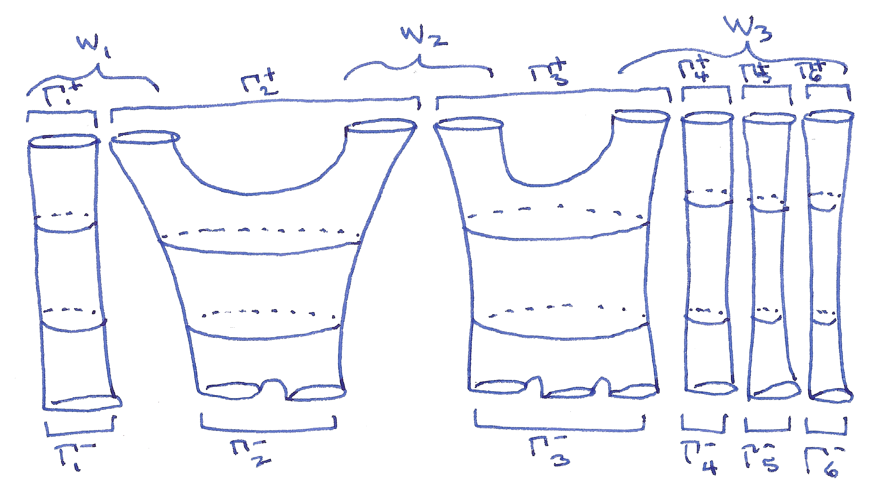
Figure 1. A typical collection of curves in $\widehat{X}$ contributing to the coefficient $\langle\Phi^{3}(w_{1},w_{2},w_{3}),x_{\Gamma_{1}^{-}}...x_{\Gamma_{6}^{-}}\rangle$.

To see that the maps $\Phi^{1},\Phi^{2},\Phi^{3},...$ define an $\mathcal{L}_{\infty}$ homomorphism, we look at the boundary of the compactified moduli space $\overline{\mathcal{M}}_{X}(\Gamma^{+};\Gamma^{-})$ for ${\operatorname{ind}}_{X,\omega}(\Gamma^{+};\Gamma^{-})=1$, with $\Gamma^{+}=(\gamma_{1},...,\gamma_{k})$. It suffices to check the relation $\widehat{\ell}_{Y^{-}}\circ\widehat{\Phi}-\widehat{\Phi}\circ\widehat{\ell}_{Y^{+}}=0$ on elements $x_{\gamma_{1}}\odot...\odot x_{\gamma_{k}}\in\overline{S}\mathcal{A}_{Y^{+}}$, with $\widehat{\Phi}:\overline{S}\mathcal{A}_{Y^{+}}\rightarrow\overline{S}\mathcal{A}_{Y^{-}}$ the induced map on bar complexes. This follows because the coefficient of $x_{\Gamma^{-}}$ in this relation precisely corresponds to the count of points in $\partial\overline{\mathcal{M}}_{X}(\Gamma^{+};\Gamma^{-})$.

The filtered $\mathcal{L}_{\infty}$ algebra ${{\operatorname{CHA}}}(Y)$ is in independent of the choice of almost complex structure and all other choices, up to filtered $\mathcal{L}_{\infty}$ homotopy equivalence. To see this, consider for example two different versions of the cobordism map $\Phi:{{\operatorname{CHA}}}(Y^{+})\rightarrow{{\operatorname{CHA}}}(Y^{-})$ defined by two different almost complex structures $J_{0}$ and $J_{1}$. We can pick a $1$-parameter family of almost complex structures $J_{t}$ joining $J_{0}$ and $J_{1}$, and consider a $t$-parametrized analogue of the map $\Phi$ defined by counting solutions to an appropriate $t$-parametrized moduli space of curves in $X$. According to [18, Thm 2.4.5], the resulting algebraic output is a homotopy between the rational SFT potentials associated to $J_{0}$ and $J_{1}$, formulated in terms of a certain Hamilton-Jacobi differential equation. In our setup, this translates precisely to a filtered $\mathcal{L}_{\infty}$ homotopy between filtered $\mathcal{L}_{\infty}$ homomorphisms as in §2. Note that this implies in particular that the homology level versions of ${{\operatorname{CHA}}}(Y)$ and $\mathcal{B}{{\operatorname{CHA}}}(Y)$ are well-defined up to isomorphism over $\Lambda_{\geq 0}$.

Remark 3.13.

The fact that ${{\operatorname{CHA}}}(Y)$ and $\mathcal{B}{{\operatorname{CHA}}}(Y)$ have well-defined torsion over $\Lambda_{\geq 0}$ is plausible, since we are considering these as invariants of the strict contact manifold $(Y,\alpha)$ up to strict contactomorphism. If instead we were to consider general contactomorphisms, we could only expect equivalences over the Novikov field $\Lambda$.

3.4.3. The $\mathcal{L}_{\infty}$ structure on linearized contact homology

Given a symplectic filling $(X,\omega)$, we can also linearize the $\mathcal{L}_{\infty}$ structure on ${{\operatorname{CHA}}}(X)$ to get a much smaller $\mathcal{L}_{\infty}$ structure whose underlying chain complex is ${\operatorname{CH}}_{{\operatorname{lin}}}(X)$. More precisely, we define operations $\ell^{k}_{{\operatorname{lin}}}:\odot^{k}\mathcal{X}\rightarrow\mathcal{X}$ which together form an $\mathcal{L}_{\infty}$ algebra structure on $s^{-1}\mathcal{X}$, and such that $\ell^{1}_{{\operatorname{lin}}}=\partial_{{\operatorname{lin}}}$ is the linearized contact homology differential.

As a special case of the cobordism map $\Phi$ from §3.4.2, the filling $X$ induces an $\mathcal{L}_{\infty}$ augmentation $\epsilon:{{\operatorname{CHA}}}(Y)\rightarrow\Lambda_{\geq 0}$. Let $w_{1},...,w_{k}\in\mathcal{A}_{Y}$ be words as above. We define an $\mathcal{L}_{\infty}$ homomorphism $F^{\epsilon}:\mathcal{A}\rightarrow\mathcal{A}$ by

$$F^{\epsilon;k}(w_{1},...,w_{k})$$

$$= \sum_{\begin{subarray}{c}J_{1}\sqcup...\sqcup J_{m}\sqcup K=\{1,...,N\}\\ A_{1},...,A_{m}\;:\;A_{i}\in H_{2}(X,\Gamma_{i}^{+}\cup\varnothing;\mathbb{Z})\end{subarray}}\#\overline{\mathcal{M}}_{X,A_{1}}(\Gamma_{1}^{+};\varnothing)...\#\overline{\mathcal{M}}_{X,A_{m}}(\Gamma_{m}^{+};\varnothing)T^{[\omega]\cdot(A_{1}+...+A_{m})}x_{\Gamma_{K}},$$

where $\Gamma_{i}^{+}\in\mathfrak{S}_{|J_{i}|}(Y,\alpha)$ corresponds to $J_{i}$ for $i=1,...,m$, $\Gamma_{K}\in\mathfrak{S}_{|K|}(Y,\alpha)$ corresponds to $K$, and the sum is over all partitions $J_{1}\sqcup...\sqcup J_{m}\sqcup K=\{1,...,N\}$ with the property that the graph $G(I_{1},...,I_{k};J_{1},...,J_{m})$ is simply connected. Note that the map $F^{\epsilon;1}$ agrees with the automorphism of $\mathcal{A}$ defined in §3.4.1 (and denoted by $F^{\epsilon}$ there). Moreover, the $\mathcal{L}_{\infty}$ homomorphism $F^{\epsilon}$ is invertible, with inverse $F^{-\epsilon}$. We can therefore define a new $\mathcal{L}_{\infty}$ structure on $s^{-1}\mathcal{A}$ via $\widehat{\ell}^{\epsilon}:=\widehat{F^{\epsilon}}\circ\widehat{\ell}\circ\widehat{F^{-\epsilon}}$. This corresponds to defining new $\mathcal{L}_{\infty}$ operations $\ell^{\epsilon;1},\ell^{\epsilon;2},\ell^{\epsilon;3},...$, which have the property that $\pi_{0}\circ\ell_{\epsilon}^{k}=0$ for each $k$. Therefore, we can restrict the operations $\ell^{\epsilon;k}$ to inputs from $\mathcal{X}$ and post-compose with the projection $\pi_{1}$ to get $\mathcal{L}_{\infty}$ operations $\ell^{k}_{{{\operatorname{lin}}}}:\odot^{k}\mathcal{X}\rightarrow\mathcal{X}$ for $k=1,2,3,...$. In particular, the differential $\ell^{1}_{{{\operatorname{lin}}}}$ agrees with the linearized contact homology differential $\partial_{{{\operatorname{lin}}}}$ from before.

As in the case of the linearized contact homology differential, we can interpret the $\mathcal{L}_{\infty}$ operations on ${\operatorname{CH}}_{{\operatorname{lin}}}$ more geometrically as follows. The structure coefficient $\langle\ell^{k}_{{\operatorname{lin}}}(x_{\gamma_{1}},...,x_{\gamma_{k}}),x_{\eta}\rangle$ counts rational curves in the symplectization of $Y$ with $k$ positive ends $\gamma_{1},...,\gamma_{k}$ and $1$ negative end $\eta$, plus some number of additional anchors in $X$. Unlike the case of $\partial_{{\operatorname{lin}}}$, the symplectization level can actually be disconnected, with one nontrivial component and some number of trivial cylinders, and the anchors in $X$ can have multiple positive ends. See Figure 2 for a cartoon.

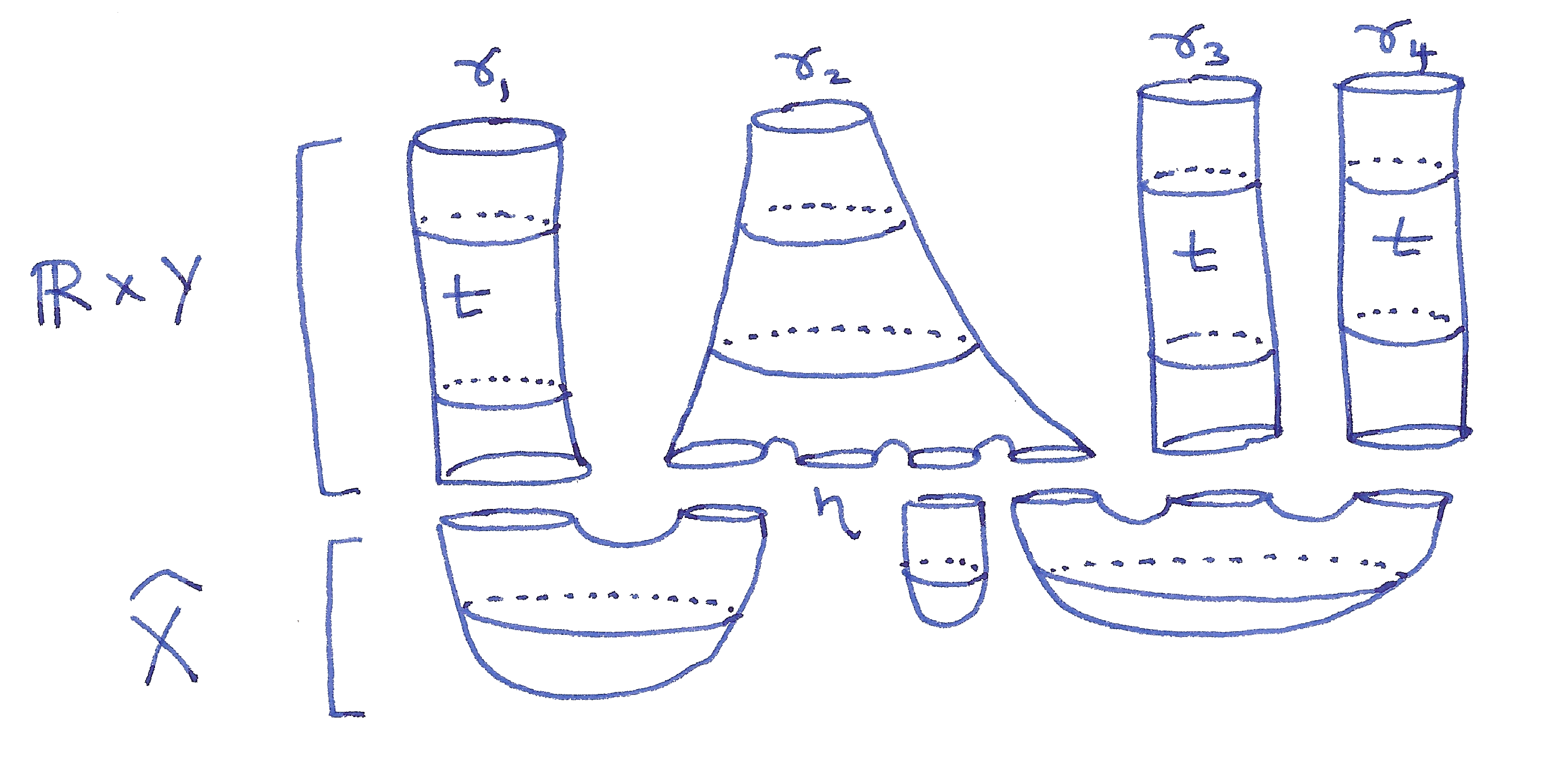
Figure 2. A typical configuration contributing to the coefficient $\langle\ell^{4}_{{{\operatorname{lin}}}}(x_{\gamma_{1}},x_{\gamma_{2}},x_{\gamma_{3}},x_{\gamma_{4}}),x_{\eta}\rangle$. Here the cylinders labeled by $t$ are trivial cylinders.

Suppose that $(X_{0},\omega_{0})$ and $(X_{1},\omega_{1})$ are symplectic fillings, with a symplectic embedding $X_{0}\hookrightarrow X_{1}$ such that $X_{1}\setminus X_{0}$ is an exact symplectic cobordism. By linearizing the $\mathcal{L}_{\infty}$ cobordism map $\Phi:{{\operatorname{CHA}}}(\partial^{+}X_{1})\rightarrow{{\operatorname{CHA}}}(\partial^{+}X_{0})$, we get an $\mathcal{L}_{\infty}$ homomorphism

$$\Phi_{{{\operatorname{lin}}}}:{{\operatorname{CHA}}}(X_{1})\rightarrow{{\operatorname{CHA}}}(X_{0}),$$

well-defined up to filtered $\mathcal{L}_{\infty}$ homotopy. In general, for $(X,\omega)$ a symplectic filling, the filtered $\mathcal{L}_{\infty}$ algebra ${\operatorname{CH}}_{{\operatorname{lin}}}(X)$ is a symplectomorphism invariant of $(X,\omega)$, up to filtered $\mathcal{L}_{\infty}$ homotopy equivalence.

4. The Cieliebak–Latschev element

A non-exact symplectic cobordism $(X,\omega)$ between $(Y^{+},\alpha^{+})$ and $(Y^{-},\alpha^{-})$ does not generally induce chain maps

$${{\operatorname{CHA}}}(Y^{+})\rightarrow{{\operatorname{CHA}}}(Y^{-}),$$

$${\operatorname{CH}}_{{\operatorname{lin}}}(Y^{+})\rightarrow{\operatorname{CH}}_{{\operatorname{lin}}}(Y^{-}),$$

let alone $\mathcal{L}_{\infty}$ homomorphisms. The basic issue is that an index $1$ curve in $X$ can break into a configuration involving “reverse anchors”, i.e. rational curves in $X$ with only negative ends. These reverse anchors, which pose an obstruction to defining a chain map, are ruled out for exact symplectic cobordisms exact by Stokes’ theorem. Nevertheless, inspired by [22], Cieliebak–Latschev observed that we can still define transfer maps, provided we appropriately deform the target. In fact, the reverse anchors assemble to define a Maurer–Cartan element $\mathfrak{cl}$ in ${{\operatorname{CHA}}}(Y^{-})$, and there is an $\mathcal{L}_{\infty}$ homomorphism

$$\Phi:{{\operatorname{CHA}}}(Y^{+})\rightarrow{{\operatorname{CHA}}}_{\mathfrak{cl}}(Y^{-}),$$

where the latter denotes the $\mathcal{L}_{\infty}$ structure with deformed operations $\ell^{1}_{\mathfrak{cl}},\ell^{2}_{\mathfrak{cl}},\ell^{3}_{\mathfrak{cl}},...$ as in §2.3.

More precisely, we define $\mathfrak{cl}\in{{\operatorname{CHA}}}(Y^{-})$ by

$$\mathfrak{cl}:=\sum_{\begin{subarray}{c}\Gamma^{-}\in\mathfrak{S}(Y^{-},\alpha^{-})\\ A\in H_{2}(X,\varnothing\cup\Gamma^{-};\mathbb{Z})\end{subarray}}\#\overline{\mathcal{M}}_{X,A}(\varnothing;\Gamma^{-})\frac{T^{[\omega]\cdot A}}{\mu_{\Gamma^{-}}\kappa_{\Gamma^{-}}}x_{\Gamma^{-}}.$$

To see that this is a Maurer–Cartan element, one analyzes the boundary strata of the spaces $\overline{\mathcal{M}}_{X,A}(\varnothing;\Gamma^{-})$ in the case that ${\operatorname{ind}}_{X,A}(\varnothing;\Gamma^{-})=1$. Namely, each boundary stratum is a two-level building, with an index $0$ level in $X$ and an index $1$ level in the symplectization of $Y$, and this contributes a term of the form $\ell^{k}(\mathfrak{cl},...,\mathfrak{cl})$. A similar analysis, looking at moduli spaces of index $1$ curves in $X$, confirms that $\Phi$ is an $\mathcal{L}_{\infty}$ homomorphism from ${{\operatorname{CHA}}}(Y^{+})$ to ${{\operatorname{CHA}}}_{\mathfrak{cl}}(Y^{-})$. Arguing as in §3.4.1, one can also show that $\mathfrak{cl}$ is independent of any choices up to gauge equivalence.

Remark 4.1.

We can view a symplectic filling $(X,\omega)$ of $(Y,\alpha)$ as a cobordism with negative end the empty set and trivial Cieliebak–Latschev element. In particular, in this case the $\mathcal{L}_{\infty}$ augmentation $\epsilon:{{\operatorname{CHA}}}(Y)\rightarrow\Lambda_{\geq 0}$ is defined without any deformation.

Now suppose that $(X_{0},\omega_{0})$ is a symplectic filling of $(Y^{-},\alpha^{-})$, and let $(X,\omega)$ be a (possibly non-exact) symplectic cobordism with positive end $(Y^{+},\alpha^{+})$ and negative end $(Y^{-},\alpha^{-})$. In this situation we have a linearized version of $\mathfrak{cl}\in{{\operatorname{CHA}}}(Y^{-})$, which is a Maurer–Cartan element ${\mathfrak{cl}_{{\operatorname{lin}}}}$ for the $\mathcal{L}_{\infty}$ structure on ${\operatorname{CH}}_{{\operatorname{lin}}}(X_{0})$. Namely, we push forward $\mathfrak{cl}$ under the $\mathcal{L}_{\infty}$ homomorphism $F^{\epsilon}:{{\operatorname{CHA}}}(Y^{-})\rightarrow{{\operatorname{CHA}}}(Y^{-})$, and then set

$${\mathfrak{cl}_{{\operatorname{lin}}}}:=\pi_{1}(F^{\epsilon}_{*}(\mathfrak{cl}))\in{\operatorname{CH}}_{{\operatorname{lin}}}(X_{0}).$$

Let ${\operatorname{CH}}_{{\operatorname{lin,{\mathfrak{cl}_{{\operatorname{lin}}}}}}}(X_{0})$ denote the $\mathcal{L}_{\infty}$ structure on ${\operatorname{CH}}_{{\operatorname{lin}}}(X_{0})$ deformed by ${\mathfrak{cl}_{{\operatorname{lin}}}}$. We can also linearize $\Phi$ to define an $\mathcal{L}_{\infty}$ homomorphism $\Phi_{{\operatorname{lin}}}:{\operatorname{CH}}_{{\operatorname{lin}}}(X_{0}\circledcirc X)\rightarrow{\operatorname{CH}}_{{{\operatorname{lin}}},{\mathfrak{cl}_{{\operatorname{lin}}}}}(X_{0})$. See Figure 3.

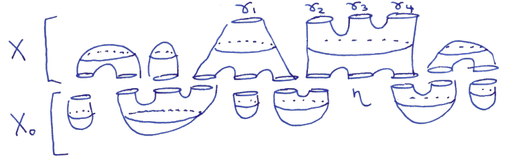
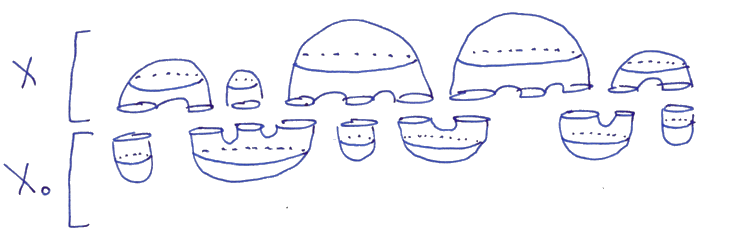
Figure 3. Left: a typical configuration contributing to the coefficient $\langle\Phi^{4}_{{{\operatorname{lin}}}}(x_{\gamma_{1}},x_{\gamma_{2}},x_{\gamma_{3}},x_{\gamma_{4}}),x_{\eta}\rangle$, in the case of a non-exact symplectic cobordism $X$. Right: a typical configuration contributing to the Maurer–Cartan element ${\mathfrak{cl}_{{\operatorname{lin}}}}\in{\operatorname{CH}}_{{\operatorname{lin}}}(X_{0})$.

Now consider the case that $(M,\beta)=(X^{-},\omega^{-})\circledcirc(X^{+},\omega^{+})$ is a closed symplectic manifold which decomposes into a symplectic filling $(X^{-},\omega^{-})$ and a symplectic cap $(X^{+},\omega^{+})$ with common contact boundary $(Y,\alpha)$. For simplicity, assume there are no rigid closed curves in $(X^{-},\omega^{-})$ or $(X^{+},\omega^{+})$ individually. We have the Cieliebak–Latschev element $\mathfrak{cl}\in{{\operatorname{CHA}}}(Y)$, and the augmentation $\epsilon:{{\operatorname{CHA}}}(Y)\rightarrow\Lambda_{\geq 0}$ induced by the filling $X^{-}$. We can also consider the genus zero Gromov–Witten invariant

$${\operatorname{GW}}_{M}=\sum_{A\in H_{2}(M;\mathbb{Z})}T^{[\omega]\cdot A}{\operatorname{GW}}_{M,A}\in\Lambda_{\geq 0},$$

where for a homology class $A\in H_{2}(M;\mathbb{Z})$ we put ${\operatorname{GW}}_{M,A}=\#\overline{\mathcal{M}}_{M,A}\in\mathbb{Q}$. In this situation, by analyzing what happens when we neck-stretch closed curves in $M$ along the contact-type hypersurface $Y$, we find the following relation:

$$\epsilon_{*}(\mathfrak{cl})={\operatorname{GW}}_{M},$$

where $\epsilon_{*}(\mathfrak{cl})\in\Lambda_{\geq 0}$ is defined as in §2.3 by

$$\epsilon_{*}(\mathfrak{cl})=\sum_{k=1}^{\infty}\frac{1}{k!}\epsilon^{k}(\underbrace{\mathfrak{cl},...,\mathfrak{cl}}_{k})=\pi_{1}\widehat{\epsilon}(\exp(\mathfrak{cl})).$$

Similarly, we have

$$(\epsilon_{{\operatorname{lin}}})_{*}({\mathfrak{cl}_{{\operatorname{lin}}}})={\operatorname{GW}}_{M}.$$

In the next section we define various generalizations of the $\mathcal{L}_{\infty}$ augmentation $\epsilon$ which count curves with various additional geometric constraints. The same neck-stretching argument gives

$$(\epsilon_{{\operatorname{lin}}})_{*}\Langle\mathcal{T}^{m}p\Rangle({\mathfrak{cl}_{{\operatorname{lin}}}})={\operatorname{GW}}_{M}\Langle\mathcal{T}^{m}p\Rangle,$$

and more generally

$$\epsilon_{*}\Langle(\mathcal{T}^{m^{1}_{1}}p_{1},...,\mathcal{T}^{m^{1}_{b_{1}}}p_{1}),...,(\mathcal{T}^{m^{r}_{1}}p_{r},...,\mathcal{T}^{m^{r}_{b_{r}}}p_{r})\Rangle(\mathfrak{cl})$$

$$={\operatorname{GW}}_{M}\Langle(\mathcal{T}^{m^{1}_{1}}p_{1},...,\mathcal{T}^{m^{1}_{b_{1}}}p_{1}),...,(\mathcal{T}^{m^{r}_{1}}p_{r},...,\mathcal{T}^{m^{r}_{b_{r}}}p_{r})\Rangle,$$

provided that there are no rigid closed curves in $(X^{+},\omega^{-})$ or $(X^{+},\omega^{+})$ satisfying the same constraints (so that closed curves are forced to split nontrivially under neck stretching). This will be used in §6.2.3 to give upper bounds on the corresponding capacities.

In some cases we can make a more refined statement at the level of individual homology classes. For example, suppose that $X^{-}$ is a symplectic filling of $Y$ such that $H_{1}(Y;\mathbb{Z})=H_{2}(Y;\mathbb{Z})=H_{2}(X^{-})=0$ (e.g. $X^{-}$ is a star-shaped domain). Let $X^{+}$ be a cap of $Y$, and set $M=X^{-}\circledcirc X^{+}$. In this situation, each homology group $H_{2}(X^{+};\varnothing\cup\Gamma^{-};\mathbb{Z})$ is naturally identified with $H_{2}(X^{+};\mathbb{Z})$, and the inclusion $H_{2}(X^{+};\mathbb{Z})\rightarrow H_{2}(M;\mathbb{Z})$ is an isomorphism. Under these identifications, curves in $X^{+}$ define classes in $H_{2}(M;\mathbb{Z})$, and we have

$$\widehat{\ell}(\exp(\mathfrak{cl})_{A})=0,$$

where $\exp(\mathfrak{cl})_{A}$ denotes the component of $\exp(\mathfrak{cl})$ in the class $A\in H_{2}(M;\mathbb{Z})$. Moreover, we have the relation

$$\epsilon_{*}(\exp(\mathfrak{cl})_{A})=T^{[\omega]\cdot A}{\operatorname{GW}}_{M,A},$$

and similarly for the other relations discussed above.

5. Geometric constraints and augmentations

Let $(Y,\alpha)$ be a strict contact manifold, with symplectic filling $(X,\omega)$. As discussed in §3.4, the filling induces an $\mathcal{L}_{\infty}$ augmentation $\epsilon:{{\operatorname{CHA}}}(Y)\rightarrow\Lambda_{\geq 0}$, which is used to define the linearized $\mathcal{L}_{\infty}$ algebra ${\operatorname{CH}}_{{\operatorname{lin}}}(X)$. Recall that the augmentation $\epsilon$ counts index $0$, (possibly disconnected) rational curves in $X$. In this section, we define various other $\mathcal{L}_{\infty}$ augmentations ${{\operatorname{CHA}}}(Y)\rightarrow\Lambda_{\geq 0}$. These can be interpreted as counting rational curves in $X$ which become rigid after imposing additional geometric constraints:

• requiring curves to pass through $r$ generic points $p_{1},...p_{r}\in X$

• requiring curves to pass through a chosen point in $p\in X$ with an order $m$ local tangency constraint at that point

• requiring curves to have an order $b$ self-contact singularity at a chosen point $p\in X$ (e.g. $b=2$ corresponds to having a node at $p$),

as well as hybrids of these conditions. By counting curves in $X$ which satisfy these extra constraints, we get corresponding $\mathcal{L}_{\infty}$ augmentations ${{\operatorname{CHA}}}(Y)\rightarrow\Lambda_{\geq 0}$, denoted by $\epsilon\Langle p_{1},...,p_{r}\Rangle$, $\epsilon\Langle\mathcal{T}^{m}p\Rangle$, and $\epsilon\Langle\underbrace{p,...,p}_{b}\Rangle$ respectively. The first type of constraint is a standard part of symplectic field theory and is described (in slightly different language) in [18]. The second type of constraint is based on the setup of Cieliebak–Mohnke [7]. The local tangency constraints we consider are closely related to but subtly different from a gravitational descendant condition at a point (see Remark 5.5 for more details). The third type of constraint is most naturally formulated in terms of curves in a multiple blow-up of $X$ in a specified homology class. In §5.5, we combine all of these constraints into a unified framework by considering curves in a symplectic cobordism with extra negative ends. The basic idea is to count curves with specified ends after removing small neighborhoods of points $p_{1},...,p_{r}$ from $X$. This allows us to combine constraints into general augmentations of the form $\epsilon\Langle(\mathcal{T}^{m^{1}_{1}}p_{1},...,\mathcal{T}^{m^{1}_{b_{1}}}p_{1}),...,(\mathcal{T}^{m^{r}_{1}}p_{r},...,\mathcal{T}^{m^{r}_{b_{r}}}p_{r})\Rangle$, which can all be defined within a standard SFT framework. By plugging these augmentations in the formalism of §6.1, these give rise to symplectic capacities. In §5.7, we discuss a relation between the three types of constraints, based on the fact that constraints at different points in the target space can be “pushed together” into constraints at a single point.

Remark 5.1.

The above constraints can also be posed for closed curves in say a closed symplectic manifold $(M,\beta)$, giving rise to Gromov–Witten-type invariants rather than $\mathcal{L}_{\infty}$ augmentations. We denote the corresponding curve counts in homology class $A\in H_{2}(M;\mathbb{Z})$ by

$${\operatorname{GW}}_{M,A}\Langle(\mathcal{T}^{m^{1}_{1}}p_{1},...,\mathcal{T}^{m^{1}_{b_{1}}}p_{1}),...,(\mathcal{T}^{m^{r}_{1}}p_{r},...,\mathcal{T}^{m^{r}_{b_{r}}}p_{r})\Rangle\in\mathbb{Q}.$$

Most of the above $\mathcal{L}_{\infty}$ augmentations are not stable under products with $\mathbb{C}$. Indeed, each constraint $\mathcal{T}^{m^{i}_{j}}p_{k}$ prescribes a negative end of a curve, whereas we only expect curves with one negative end to stabilize (c.f. the index computation in §1.1). The exception is the $\mathcal{L}_{\infty}$ augmentation $\epsilon\Langle\mathcal{T}^{m}p\Rangle$, which is formulated in terms of a single negative end. As such, it linearizes to an augmentation

$$\epsilon_{{\operatorname{lin}}}\Langle\mathcal{T}^{m}p\Rangle:{\operatorname{CH}}_{{\operatorname{lin}}}(X)\rightarrow\Lambda_{\geq 0}$$

which is dimensionally stable. The details are discussed in §5.4.

5.1. Point constraints

Let $(X^{2n},\omega)$ be a symplectic cobordism between $(Y^{+},\alpha^{+})$ and $(Y^{-},\alpha^{-})$. The induced $\mathcal{L}_{\infty}$ cobordism map $\Phi:{{\operatorname{CHA}}}(Y^{+})\rightarrow{{\operatorname{CHA}}}(Y^{-})$ is defined in terms of index $0$ moduli spaces $\overline{\mathcal{M}}_{X,A}(\Gamma^{+};\Gamma^{-})$. We can also consider the versions $\overline{\mathcal{M}}_{X,A,r}(\Gamma^{+};\Gamma^{-})$ with an additional $r$ (ordered) marked points freely varying in the domain. These moduli spaces come with evaluation maps ${{\operatorname{ev}}}:\overline{\mathcal{M}}_{X,A,r}(\Gamma^{+};\Gamma^{-})\rightarrow X^{\times r}$. Fixing pairwise distinct points $p_{1},...,p_{r}\in X$, we define the moduli space of curves with $r$ point constraints by

$$\overline{\mathcal{M}}_{X,A}(\Gamma^{+};\Gamma^{-})\Langle p_{1},...,p_{r}\Rangle:={{\operatorname{ev}}}^{-1}(\{p_{1}\}\times...\times\{p_{r}\}).$$

Note that each point constraint cuts down the expected dimension by $2n-2$, so $\overline{\mathcal{M}}_{X,A}(\Gamma^{+};\Gamma^{-})\Langle p_{1},...,p_{r}\Rangle$ having index $0$ corresponds to $\overline{\mathcal{M}}_{X,A,r}(\Gamma^{+};\Gamma^{-})$ having index $r(2n-2)$. The combinatorial structure of the boundary strata of $\overline{\mathcal{M}}_{X,A}(\Gamma^{+};\Gamma^{-})\Langle p_{1},...,p_{r}\Rangle$ is such that a typical element of $\partial\overline{\mathcal{M}}_{X,A}(\Gamma^{+};\Gamma^{-})\Langle p_{1},...,p_{r}\Rangle$ consists of a pseudoholomorphic building with one “main” level in $X$ and some number of levels in the symplectization $\mathbb{R}\times Y^{\pm}$. Note that the curves in the main level may be disconnected, and the point constraints $p_{1},...,p_{r}$ are distributed arbitrarily between the different components in $X$.

We define the point-constrained $\mathcal{L}_{\infty}$ cobordism map $\Phi\Langle p_{1},...,p_{r}\Rangle:{{\operatorname{CHA}}}(Y^{+})\rightarrow{{\operatorname{CHA}}}(Y^{-})$ in the same way that we defined the $\mathcal{L}_{\infty}$ cobordism map $\Phi:{{\operatorname{CHA}}}(Y^{+})\rightarrow{{\operatorname{CHA}}}(Y^{-})$, but now imposing the point constraints $p_{1},...,p_{r}$. In particular, if $(X,\omega)$ is a symplectic filling, we get an $\mathcal{L}_{\infty}$ augmentation

$$\epsilon\Langle p_{1},...,p_{r}\Rangle:{{\operatorname{CHA}}}(Y)\rightarrow\Lambda_{\geq 0}.$$

As in §3.4, it follows from the general invariance properties of rational symplectic field theory that $\epsilon\Langle p_{1},...,p_{r}\Rangle$ is independent of all choices, including the precise locations of the points $p_{1},...,p_{r}\in X$, up to (filtered) $\mathcal{L}_{\infty}$ homotopy.

Remark 5.2.

More generally, instead of requiring curves to pass through points $p_{1},...,p_{r}$, we could require them to pass through $r$ chosen cycles in $X$. However, in this paper we will only make use of the point class, since this is the only homology class relevant to all symplectic fillings regardless of their topological type.

Remark 5.3.

There is another $\mathcal{L}_{\infty}$ augmentation ${{\operatorname{CHA}}}(Y)\rightarrow\Lambda_{\geq 0}$ which is very similar to $\epsilon\Langle p_{1},...,p_{r}\Rangle$ but does not reference the filling $(X,\omega)$. It is defined in the same way except that we pick the points $p_{1},...,p_{r}$ to lie in $\mathbb{R}\times Y$ rather than $X$, and we count curves in $\mathbb{R}\times Y$ rather than in $X$. These curves still have no negative ends, and here we think of $\mathbb{R}\times Y$ as a symplectic cobordism rather than a symplectization (i.e. we do not quotient by translations in the target). In some cases these two $\mathcal{L}_{\infty}$ augmentations coincide. Namely, if for every $\Gamma^{+}\in\mathfrak{S}(Y,\alpha)$ we have $\#\overline{\mathcal{M}}_{X}(\Gamma^{+};\varnothing)=0$, then by a neck-stretching argument the relevant curves in $\widehat{X}$ are in correspondence with curves in $\mathbb{R}\times Y$.

For example, this holds for ellipsoids $E(a_{1},...,a_{n})$ for index reasons. More generally, if we have $c_{1}(X,\omega)=0$ and every Reeb orbit $\gamma$ of $Y$ satisfies ${{\operatorname{CZ}}}(\gamma)>|n-3|$, then for all $\Gamma^{+}=(\gamma_{1}^{+},...,\gamma_{k}^{+})\in\mathfrak{S}(Y,\alpha)$ we have ${\operatorname{ind}}\;\overline{\mathcal{M}}_{X}(\Gamma^{+};\varnothing)>0$, so there are no rigid genus zero anchors in $X$. Indeed, we have

$${\operatorname{ind}}\;\overline{\mathcal{M}}_{X}(\Gamma^{+};\varnothing)=(n-3)(2-k)+\sum_{i=1}^{k}{{\operatorname{CZ}}}(\gamma_{i}^{+})>(n-3)(2-k)+k|n-3|\geq 0.$$

For $r=1$, the $\mathcal{L}_{\infty}$ augmentation $\epsilon\Langle p\Rangle:{{\operatorname{CHA}}}(Y)\rightarrow\Lambda_{\geq 0}$ induces a linearized $\mathcal{L}_{\infty}$ augmentation $\epsilon_{{\operatorname{lin}}}\Langle p\Rangle:{\operatorname{CH}}_{{\operatorname{lin}}}(X)\rightarrow\Lambda_{\geq 0}$. As mentioned in the introduction, its first component $\epsilon_{{\operatorname{lin}}}^{1}\Langle p\Rangle:{\operatorname{CH}}_{{\operatorname{lin}}}(X)\rightarrow\Lambda_{\geq 0}$ is part of the SFT model for symplectic cohomology considered in [4]. For $r\geq 2$ the $\mathcal{L}_{\infty}$ augmentation $\epsilon\Langle p_{1},...,p_{r}\Rangle:{{\operatorname{CHA}}}(Y)\rightarrow\Lambda_{\geq 0}$ does not induce an $\mathcal{L}_{\infty}$ augmentation ${\operatorname{CH}}_{{\operatorname{lin}}}(X)\rightarrow\Lambda_{\geq 0}$. Indeed, even the chain map $\epsilon^{1}\Langle p_{1},...,p_{r}\Rangle:{{\operatorname{CHA}}}(X)\rightarrow\Lambda_{\geq 0}$ does not induce a chain map ${\operatorname{CH}}_{{\operatorname{lin}}}(X)\rightarrow\Lambda_{\geq 0}$. The essential reason is that an index $1$ curve in $X$ with two point constraints can degenerate into a configuration for which the marked points lie on different curve components in $X$.

5.2. Tangency constraints

Following Cieliebak–Mohnke [7, 6], we can consider curves in a symplectic cobordism $(X,\omega)$ satisfying certain local tangency constraints. Let $J$ be an admissible almost complex structure on $\widehat{X}$ which is integrable near a chosen point $p\in X$, and let $D$ be a germ of complex divisor in $\mathcal{O}p(p)$. Suppose we have a $J$-holomorphic map $u:\Sigma\rightarrow\widehat{X}$ and a marked point $z\in\Sigma$ such that $u(z)=p$. In this situation there is a well-defined notion of $u$ being tangent to $D$ of order $m$ at $z$, which one can formulate in local coordinates and then show to coordinate-independent (see [7] for details). Let $\mathcal{M}_{X,A}(\Gamma^{+};\Gamma^{-})\Langle\mathcal{T}^{m}p\Rangle$ be defined in the same way as $\mathcal{M}_{X,A}(\Gamma^{+},\Gamma^{-})$, but now with the constituent curves having one marked point $z$ which maps to $p$ and is tangent to $D$ of order $m$ at $z$. It is shown in [7, Prop 3.1] that for generic $J$ (which can be assumed to be fixed and integrable near $p$), the moduli space $\mathcal{M}_{X,A}(\Gamma^{+};\Gamma^{-})\Langle\mathcal{T}^{m}p\Rangle$ is, at least near a somewhere injective curve $u$, a smooth manifold of dimension

$$(n-3)(2-s^{+}-s^{-})+\sum_{i=1}^{s^{+}}{{\operatorname{CZ}}}(\gamma_{i}^{+})-\sum_{j=1}^{s^{-}}{{\operatorname{CZ}}}(\gamma_{j}^{-})+2c_{1}(X,\omega)\cdot A_{u}-(2n-2)-2m.$$

Note that the $\mathcal{T}^{m}p$ constraint is a real codimension $2n-2+2m$ condition. If we fix distinct points $p_{1},...,p_{r}\in X$ and a divisor germ $D_{i}$ at each $p_{i}$, for $m_{1},...,m_{r}\in\mathbb{Z}_{\geq 0}$ we can similarly define the moduli space $\mathcal{M}_{X,A}(\Gamma^{+},\Gamma^{-})\Langle\mathcal{T}^{m_{1}}p_{1},...,\mathcal{T}^{m_{r}}p_{r}\Rangle$ by considering curves with marked points $z_{1},...,z_{r}$, with $z_{i}$ mapping to $p_{i}$ and tangent to $D_{i}$ of order $m_{i}$.

Now suppose that $(X,\omega)$ is a symplectic filling of $(Y,\alpha)$. By counting index $0$ curves in compactified moduli spaces $\overline{\mathcal{M}}_{X,A}(\Gamma^{+},\varnothing)\Langle\mathcal{T}^{m_{1}}p_{1},...,\mathcal{T}^{m_{r}}p_{r}\Rangle$, we get an $\mathcal{L}_{\infty}$ augmentation $\epsilon\Langle\mathcal{T}^{m_{1}}p_{1},...,\mathcal{T}^{m_{r}}p_{r}\Rangle:{{\operatorname{CHA}}}(Y)\rightarrow\Lambda_{\geq 0}$. In the special case $r=1$, we also have an induced linearized $\mathcal{L}_{\infty}$ augmentation $\epsilon_{{\operatorname{lin}}}\Langle\mathcal{T}^{m}p\Rangle:{\operatorname{CH}}_{{\operatorname{lin}}}(X)\rightarrow\Lambda_{\geq 0}$.

Remark 5.4.

In a closed symplectic manifold, the analogous counts of closed curve with tangency constraints are considered in [48]. It is shown in that setting that these give enumerative invariants which can be defined for all semipositive symplectic manifolds using only classical transversality techniques.

Remark 5.5 (on the relationship between tangency constraints and gravitational descendants).

Here we compare curve counts with the tangency constraint $\Langle\mathcal{T}^{m}p\Rangle$ to the gravitational descendant condition $\Langle\psi^{m}p\Rangle$. For simplicity, assume that $(M^{2n},\beta)$ is a closed symplectic manifold, and let $A\in H_{2}(M;\mathbb{Z})$ be a homology class such that

$${\operatorname{ind}}_{M,A}=2n-6+2c_{1}(M,\beta)\cdot A-(2n-2)-2m=0.$$

In the context of algebraic Gromov–Witten theory, recall that one defines ${\operatorname{GW}}_{M,A}\Langle\psi^{m}p\Rangle\in\mathbb{Q}$ as follows. Consider the space $\overline{\mathcal{M}}_{M,A,1}$ of genus zero stable maps to $M$ in the homology class $A$ with one marked point. This space comes with an evaluation map ${{\operatorname{ev}}}:\overline{\mathcal{M}}_{M,A,1}\rightarrow\mathbb{CP}^{2}$ and a complex line bundle $\mathbb{L}\rightarrow\overline{\mathcal{M}}_{M,A,1}$ whose fiber over a curve is the cotangent space to the curve at the marked point. We then set

$${\operatorname{GW}}_{M,A}\Langle\psi^{m}p\Rangle:=\int_{[\overline{\mathcal{M}}_{M,A}]^{{\operatorname{vir}}}}{{\operatorname{ev}}}^{*}([p]^{\vee})\cup\underbrace{c_{1}(\mathbb{L})\cup...\cup c_{1}(\mathbb{L})}_{m},$$

where $[p]^{\vee}\in H^{2n}(M;\mathbb{Q})$ denotes the point class and $[\overline{\mathcal{M}}_{M,A}]^{{\operatorname{vir}}}\in H_{2n-4+2c_{1}(M,\beta)\cdot A}(M;\mathbb{Q})$ is the virtual fundamental class. The case of open curves is more subtle, since then $\mathbb{L}$ is a line bundle over a space with codimension one boundary, but it does also appear in the literature (see for example [17, 52, 19]). Now suppose that $D$ is a smooth divisor passing through $p\in M$. In [25] (see also [60]) it is observed that the line bundle $\mathbb{L}^{\otimes k}$ for $k\in\mathbb{Z}_{>0}$ has a partially defined section $\sigma_{k}$, given by the $k$-jet of a curve at the marked point in the direction normal to $D$. The intersection of the locus ${{\operatorname{ev}}}^{-1}(p)\cap\sigma_{1}^{-1}(0)\cap...\cap\sigma_{m}^{-1}(0)$ with the main stratum $\mathcal{M}_{M,A,1}$ consists of curves with smooth domain which are tangent to $D$ to order $m$ at the marked point. The count of such curves would give precisely $m!{\operatorname{GW}}_{M,A}\Langle\psi^{m}p\Rangle$, provided we knew that the sections $\sigma_{1},...,\sigma_{m}$ were sufficiently transverse and nonvanishing along the boundary strata $\overline{\mathcal{M}}_{M,A,1}\setminus\mathcal{M}_{M,A,1}$. However, it turns out that these sections always vanish on the boundary strata, and this typically gives additional contributions to the descendant invariant.

As a simple example, we have $2!{\operatorname{GW}}_{\mathbb{CP}^{1},{\operatorname{deg}}=2}\Langle\psi^{2}p\Rangle=1/2$, which follows easily from the genus zero topological recursion formula (see for example [41]). By contrast, we have ${\operatorname{GW}}_{\mathbb{CP}^{1},{\operatorname{deg}}=2}\Langle\mathcal{T}^{2}p\Rangle=0$. In fact, the compactified moduli space $\overline{\mathcal{M}}_{\mathbb{CP}^{1},{\operatorname{deg}}=2}\Langle\mathcal{T}^{2}p\Rangle$ is empty, essentially because there are no degree two Hurwitz maps $\mathbb{CP}^{1}\rightarrow\mathbb{CP}^{1}$ with an order three branch point over $p$. As a slightly more interesting example, we have $4!{\operatorname{GW}}_{\mathbb{CP}^{2},2[L]}\Langle\psi^{4}p\Rangle=3$, whereas ${\operatorname{GW}}_{\mathbb{CP}^{2},2[L]}\Langle\mathcal{T}^{4}p\Rangle=1$ (see §5.7 below). One can show that discrepancies in both cases come from a configuration with two degree $1$ curves joined by a central ghost component containing one marked point.

Nevertheless, at least in the case of a global divisor, Gathmann [25] gives explicit descriptions of the extra boundary contributions occurring in the descendant invariants, described in terms of “comb configurations” related to the ghost configurations above. This is related to the general fact that relative Gromov–Witten invariants can be reduced to absolute Gromov–Witten invariants, possibly with gravitational descendants (c.f. [44, 51]). It might also be possible to extend this approach to the local divisor case in order to give explicit descriptions of the descendant invariants ${\operatorname{GW}}_{M,A}\Langle\psi^{m}p\Rangle$ in terms of the tangency invariants ${\operatorname{GW}}_{M,A}\Langle\mathcal{T}^{m}p\Rangle$, plus extra discrepancy configurations.

Example 5.6.

We consider the example of the two-ball $B^{2}$. Let $\alpha_{1},\alpha_{2},\alpha_{3},...$ denote the Reeb orbits of $\partial B^{2}$. Firstly, following [4], the symplectic cochain complex ${\operatorname{SC}}(B^{2})$ over $\mathbb{K}$ has a model with the following generators

• $\check{\alpha}_{k}$ for $k\geq 1$, with $\mathcal{A}(\check{\alpha}_{k})=k$ and $|\check{\alpha}_{k}|=1-2k$

• $\hat{\alpha}_{k}$ for $k\geq 1$, with $\mathcal{A}(\hat{\alpha}_{k})=k$ and $|\hat{\alpha}_{k}=-2k$

• $e$, with $\mathcal{A}(e)=0$ and $|e|=0$.

The differential $\partial$ is given by

• $\partial(\check{\alpha}_{1})=1$

• $\partial(\check{\alpha}_{k})=\hat{\alpha}_{k-1}$ for $k\geq 2$

• $\partial(\hat{\alpha}_{k})=0$ for $k\geq 1$

• $\partial(e)=0$.

In this model the higher BV operators $\Delta_{2},\Delta_{3},...$ are trivial, while $\Delta_{1}$ is given by

• $\Delta_{1}(\check{\alpha}_{k})=k\hat{\alpha}_{k}$ for $k\geq 1$

• $\Delta_{1}(\hat{\alpha}_{k})=0$ for $k\geq 1$

• $\Delta_{1}(e)=0$.

The $S^{1}$-equivariant chain complex is given by setting ${\operatorname{SC}}_{S^{1}}(B^{2})={\operatorname{SC}}(B^{2})\otimes\mathbb{K}[u^{-1}]$ and $\partial_{S^{1}}=\partial+u\Delta_{1}$. The complex ${\operatorname{SC}}_{S^{1},+}(B^{2})$ is given by quotienting out $\mathbb{K}[u^{-1}]e$, and for each $m\geq 0$ we get a chain map $\langle u^{-m}e,\partial_{S^{1}}(-)\rangle:{\operatorname{SC}}_{S^{1},+}(B^{2})\rightarrow\mathbb{K}$ which gives the coefficient of $u^{-m}e$ after applying $\partial_{S^{1}}$.

The linearized contact homology complex ${\operatorname{CH}}_{{\operatorname{lin}}}(B^{2})$ over $\mathbb{K}$ simply has one generator $x_{\alpha_{k}}$ for each $k\geq 1$, with $\mathcal{A}(x_{\alpha_{k}})=k$ and $|x_{\alpha_{k}}|=1-2k$. For $m\geq 0$, the chain map $\epsilon_{{\operatorname{lin}}}^{1}\Langle\mathcal{T}^{m}p\Rangle:{\operatorname{CH}}_{{\operatorname{lin}}}(B^{2})\rightarrow\mathbb{K}$ counts certain Hurwitz covers of $B^{2}$ with an order $m+1$ branch point over $p\in B^{2}$, and we have $\epsilon_{{\operatorname{lin}}}^{1}\Langle\mathcal{T}^{m}p\Rangle(\alpha_{k})=1$ if $k=m+1$ and $0$ otherwise. There are also natural $\mathbb{K}$-linear inverse chain homotopy equivalences $\Phi:{\operatorname{SC}}_{S^{1},+}(B^{2})\rightarrow{\operatorname{CH}}_{{\operatorname{lin}}}(B^{2})$ and $\Psi:{\operatorname{CH}}_{{\operatorname{lin}}}(B^{2})\rightarrow{\operatorname{SC}}_{S^{1},+}(B^{2})$, with

• $\Phi(\check{\alpha}_{k})=x_{\alpha_{k}}$ for $k\geq 1$

• $\Phi(u^{-j}\check{\alpha}_{k})=0$ for $j\geq 1$

• $\Phi(u^{-j}\hat{\alpha}_{k})=0$ for $j\geq 0$ and $k\geq 1$,

and

$$\Psi(x_{\alpha_{k}})=\check{\alpha}_{k}-\tfrac{u^{-1}}{k-1}\check{\alpha}_{k-1}+\tfrac{u^{-2}}{(k-1)(k-2)}\check{\alpha}_{k-2}-...+(-1)^{k-2}\tfrac{u^{-k+2}}{(k-1)...(3)(2)}\check{\alpha}_{2}+(-1)^{k-1}\tfrac{u^{-k+1}}{(k-1)!}\check{\alpha}_{1}$$

for $k\geq 1$. Observe that the chain maps $\langle u^{-m}e,\partial_{S^{1}}(-)\rangle:{\operatorname{SC}}_{S^{1},+}(B^{2})\rightarrow\mathbb{K}$ and $\epsilon_{{\operatorname{lin}}}^{1}\Langle\mathcal{T}^{m}p\Rangle\circ\Phi:{\operatorname{SC}}_{S^{1},+}(B^{2})\rightarrow\mathbb{K}$ agree up to chain homotopy and a scalar factor $\tfrac{(-1)^{m-1}}{(m-1)!}$, and similarly for the chain maps $\langle u^{-m}e,\partial_{S^{1}}(-)\rangle\circ\Psi:{\operatorname{CH}}_{{\operatorname{lin}}}(B^{2})\rightarrow\mathbb{K}$ and $\epsilon_{{\operatorname{lin}}}^{1}\Langle\mathcal{T}^{m}p\Rangle:{\operatorname{CH}}_{{\operatorname{lin}}}(B^{2})\rightarrow\mathbb{K}.$

Remark 5.7.

The above example can in fact be generalized from $B^{2}$ to any symplectic filling $X$. Namely, Bourgeois–Oancea [5] give inverse chain homotopy equivalences $\Phi:{\operatorname{SC}}_{S^{1},+}(X)\rightarrow{\operatorname{CH}}_{{\operatorname{lin}}}(X)$ and $\Psi:{\operatorname{CH}}_{{\operatorname{lin}}}(X)\rightarrow{\operatorname{SC}}_{S^{1},+}(X)$, and we claim that the chain maps $\langle u^{-m}e,\partial_{S^{1}}(-)\rangle$ and $\epsilon_{{\operatorname{lin}}}^{1}\Langle\mathcal{T}^{m}p\Rangle$ are identified after precomposing with $\Phi$ and $\Psi$, up to the same scalar factor. Indeed, using the ideas from §5.4, we can first generalize from $B^{2}$ to the ellipsoid $E(1,S,...,S)$ for $S$ sufficiently large. Since any $X$ contains a symplectic embedding of $E(\varepsilon,\varepsilon S,...,\varepsilon S)$ for $\varepsilon>0$ sufficiently small, and since both of the above augmentations associated to $X$ can be factored as a cobordism map for $X\setminus E(\varepsilon,\varepsilon S,...,\varepsilon S)$ followed by an augmentation associated to $E(\varepsilon,\varepsilon S,...,\varepsilon S)$, this suffices. We also expect a generalization of this argument to hold at the level of $\mathcal{L}_{\infty}$ structures, although writing down the explicit chain level $\mathcal{L}_{\infty}$ structures is more involved.

5.3. Blow-up constraints

We also count curves with nodal singularities or higher order self-contact singularities. These conditions are most naturally posed by considering curves in a suitable symplectic blow-up at finitely many points. First suppose that $(M^{2n},\beta)$ is a closed symplectic manifold with $2n\geq 4$. Fix distinct points $p_{1},...,p_{r}\in X$ and let $\widetilde{X}$ denote a symplectic blow-up of $X$ at the points $p_{1},...,p_{r}$. Recall that the symplectic blow-up construction starts with a collection of disjoint Darboux balls $B_{1},...,B_{r}$, with $B_{i}$ centered at $p_{i}$ and having area $a_{i}$. Then $\widetilde{X}$ is given by removing each $B_{i}$ from $X$ and collapsing its boundary along the Hopf fibration. Note that $\widetilde{X}$ depends on the points $p_{1},...,p_{r}$ and balls $B_{1},...,B_{r}$ up to symplectomorphism, but not up to symplectic deformation equivalence. Each collapsed boundary $\partial B_{i}$ gives rise to an exceptional divisor $\mathcal{E}_{i}\subset\widetilde{X}$, which is a symplectically embedded copy of $\mathbb{CP}^{n-1}$ whose line $L_{i}\subset\mathcal{E}_{i}$ has area $a_{i}$. Note that the homology group $H_{2}(\widetilde{X};\mathbb{Z})$ naturally splits as $H_{2}(X;\mathbb{Z})\oplus\mathbb{Z}\langle[L_{1}],...,[L_{r}]\rangle$, and we have $[\mathcal{E}_{i}]\cdot[L_{i}]=(-1)^{n-1}[pt]$, where $[pt]\in H_{0}(\widetilde{X};\mathbb{Z})$ is the point class. Therefore we can uniquely write any class $\widetilde{A}$ in $H_{2}(\widetilde{X};\mathbb{Z})$ as $\widetilde{A}=A+C_{1}[L_{1}]+...+C_{r}[L_{r}]$ for $C_{1},...,C_{r}\in\mathbb{Z}$, where $\sum_{i=1}^{r}C_{i}[L_{i}]$ is the “exceptional part” of $\widetilde{A}$.

For $b_{1},...,b_{r}\geq 1$, we introduce the following notation:

$${\operatorname{GW}}_{X}\Langle\underbrace{(p_{1},...,p_{1})}_{b_{1}},...,\underbrace{(p_{r},...,p_{r})}_{b_{r}}\Rangle:=\sum_{A\in H_{2}(X;\mathbb{Z})}T^{[\omega]\cdot A]}{\operatorname{GW}}_{X,A}\Langle\underbrace{(p_{1},...,p_{1})}_{b_{1}},...,\underbrace{(p_{r},...,p_{r})}_{b_{r}}\Rangle,$$

where ${\operatorname{GW}}_{X,A}\Langle\underbrace{(p_{1},...,p_{1})}_{b_{1}},...,\underbrace{(p_{r},...,p_{r})}_{b_{r}}\Rangle$ is defined to be $b_{1}!...b_{r}!{\operatorname{GW}}_{\widetilde{X},A-b_{1}[L_{1}]-...-b_{r}[L_{r}]}$. Here the extra combinatorial factor $b_{1}!...b_{r}!$ has the effect of ordering the points mapping to each exceptional divisor $\mathcal{E}_{i}$, which is convenient since the marked points in the definition of ${\operatorname{GW}}_{X,A}\Langle p_{1},...,p_{r}\Rangle$ are also ordered. Note that the Novikov exponent $T^{[\omega]\cdot A}$ ignores the exceptional part $-b_{1}[L_{1}]-...-b_{r}[L_{r}]$, and hence is independent of the sizes $a_{i}$ of the blow-up, which we think of as being arbitrarily small.

Now suppose that $(X,\omega)$ is a symplectic cobordism between $(Y^{+},\alpha^{+})$ and $(Y^{-},\alpha^{-})$. We can define an $\mathcal{L}_{\infty}$ homomorphism

$$\Phi\Langle\underbrace{(p_{1},...,p_{1})}_{b_{1}},...,\underbrace{(p_{r},...,p_{r})}_{b_{r}}\Rangle:{{\operatorname{CHA}}}(Y^{+})\rightarrow{{\operatorname{CHA}}}(Y^{-})$$

as follows. The homology group $H_{2}(\widetilde{X},\Gamma^{+}\cup\Gamma^{-};\mathbb{Z})$ naturally splits as a direct sum of $H_{2}(X,\Gamma^{+}\cup\Gamma^{-};\mathbb{Z})$ and $\mathbb{Z}\langle[L_{1}],...,[L_{r}]\rangle$. The definition of $\Phi\Langle\underbrace{(p_{1},...,p_{1})}_{b_{1}},...,\underbrace{(p_{r},...,p_{r})}_{b_{r}}\Rangle$ is similar to that of the $\mathcal{L}_{\infty}$ homomorphism $\Phi:{{\operatorname{CHA}}}(Y^{+})\rightarrow{{\operatorname{CHA}}}(Y^{-})$ from §3.4.2, with $\Phi^{k}\Langle\underbrace{(p_{1},...,p_{1})}_{b_{1}},...,\underbrace{(p_{r},...,p_{r})}_{b_{r}}\Rangle(w_{1},...,w_{k})$ given by

$$\sum_{\begin{subarray}{c}J_{1}\sqcup...\sqcup J_{m}=\{1,...,N\}\\ \Gamma_{1}^{-},...,\Gamma_{m}^{-}\in\mathfrak{S}(Y^{-},\alpha^{-})\end{subarray}}\#\overline{\mathcal{M}}_{\widetilde{X},\widetilde{A}_{1}}(\Gamma_{1}^{+};\Gamma_{1}^{-})...\#\overline{\mathcal{M}}_{\widetilde{X},\widetilde{A}_{m}}(\Gamma_{m}^{+};\Gamma_{m}^{-})\frac{T^{[\omega]\cdot(A_{1}+...+A_{m})}b_{1}!...b_{r}!}{\mu_{\Gamma_{1}^{-}}...\mu_{\Gamma_{m}^{-}}\kappa_{\Gamma_{1}^{-}}...\kappa_{\Gamma_{m}^{-}}}x_{\Gamma_{1}^{-}}...x_{\Gamma_{m}^{-}},$$

but where the sum is now over all homology classes $\widetilde{A}_{1},...,\widetilde{A}_{m}\in H_{2}(\widetilde{X},\Gamma_{i}^{+}\cup\Gamma_{i}^{-};\mathbb{Z})$ such that the total exceptional part of $\widetilde{A}_{1}+...+\widetilde{A}_{m}$ is $-b_{1}[L_{1}]-...-b_{r}[L_{r}]$. In the case that $(X,\omega)$ is a filling of $(Y,\alpha)$, we get an $\mathcal{L}_{\infty}$ augmentation

This does not generally induce an $\mathcal{L}_{\infty}$ augmentation of ${\operatorname{CH}}_{{\operatorname{lin}}}(X)$, unless $r=1$ and $b_{1}=1$. Also, the case $b_{1}=...=b_{r}=1$ agrees with $\Phi\Langle p_{1},...,p_{r}\Rangle$ from the previous subsection.

5.4. Behavior under dimensional stabilization

Here we discuss the extent to which curve counts persist to higher dimensions. Let $(X,\omega)$ be an exact symplectic filling of $(Y,\alpha)$. We will show that the linearized contact homology $\mathcal{L}_{\infty}$ algebra ${\operatorname{CH}}_{{\operatorname{lin}}}(X)$ is invariant under taking a product with $\mathbb{C}$, in a suitable sense. Similar statements hold for the $\mathcal{L}_{\infty}$ augmentation $\epsilon\Langle\mathcal{T}^{k}p\Rangle:{\operatorname{CH}}_{{\operatorname{lin}}}(X,\omega)\rightarrow\Lambda_{\geq 0}$ and the $\mathcal{L}_{\infty}$ cobordism map ${\operatorname{CH}}_{{\operatorname{lin}}}(X^{\prime})\rightarrow{\operatorname{CH}}_{{\operatorname{lin}}}(X)$ given an exact symplectic embedding $(X,\omega)\hookrightarrow(X^{\prime},\omega^{\prime})$.

Naively, the main point is that, for a split almost complex structure, curves in the product $X\times\mathbb{C}$ are given by a product of curves in each factor, and curves in $\mathbb{C}$ effectively must be constant. However, there are a few subtleties to address before making this precise. For one, the product $X\times\mathbb{C}$ is not strictly speaking a symplectic filling, due to its noncompactness. If we replace $\mathbb{C}$ with the two-ball $B^{2}(a)$ of area $a$, then $X\times B^{2}(a)$ is compact but has corners. We can smooth the corners to obtain an honest symplectic filling, but the smoothing process is not entirely canonical. In particular, different choices of smoothings lead to different Reeb dynamics. Moreover, an admissible almost complex structure for the smoothed product is no longer split, so we cannot quite argue via the projection to the $\mathbb{C}$ factor. Another issue is that the index of a punctured curve typically changes under stabilization and can potentially become negative, meaning that stabilized curves might be irregular and disappear after a small perturbation. Since ${\operatorname{CH}}_{{\operatorname{lin}}}$ effectively involves curves with one negative end, it should stabilize in a straightforward way (in contrast to ${{\operatorname{CHA}}}$, which involves multiple negative ends). However, the $\mathcal{L}_{\infty}$ structure maps of ${\operatorname{CH}}_{{\operatorname{lin}}}$ technically count anchored curves with one negative end, hence the symplectization components could still have multiple negative ends and some care is needed.

Remark 5.8.

The papers [31, 10, 11, 46] also prove stabilization theorems similar in spirit to and provide inspiration for the one in this paper. The setup is slightly different, since those papers work directly with somewhere injective curves rather than SFT moduli spaces, and they rule out superfluous curves using an $S^{1}$-symmetry argument.

To address the above issues, we first need to discuss the smoothing process more carefully. By picking a smoothing $X\mathrel{\mathop{\times}\limits^{\vbox to-1.50694pt{\kern-2.0pt\hbox{$\scriptstyle\frown$}\vss}}}B^{2}(S)$ of $X\times B^{2}(S)$ which looks like a product on a neighborhood of $X\times\{0\}$, we can work with an admissible almost complex structure which is split on that neighborhood. This choice of smoothing produces Morse–Bott families of Reeb orbits, but we can handle this in a standard fashion by adapting the formalism to the Morse–Bott setting. By taking the neighborhood on which the smoothing looks like a product to be sufficiently wide, say $X\times B^{2}(R)$ for $S>R\gg 0$, we can arrange that any curve with ends in the slice $\widehat{X}\times\{0\}$ is either entirely contained in that slice or else has very large symplectic energy.

In more detail, given $0<R<S$, let $X\mathrel{\mathop{\times}\limits^{\vbox to-1.50694pt{\kern-2.0pt\hbox{$\scriptstyle\frown$}\vss}}}B^{2}(S)$ denote a subdomain of the naive product $X\times B^{2}(S)$ such that $X\mathrel{\mathop{\times}\limits^{\vbox to-1.50694pt{\kern-2.0pt\hbox{$\scriptstyle\frown$}\vss}}}B^{2}(S)$ is a symplectic filling with respect to the restriction of the product symplectic form, and such that it contains the product subdomain $X\times B^{2}(R)$. In particular, this means that $X\mathrel{\mathop{\times}\limits^{\vbox to-1.50694pt{\kern-2.0pt\hbox{$\scriptstyle\frown$}\vss}}}B^{2}(S)$ has smooth boundary which is a contact hypersurface. By default we think of $R$ as being arbitrarily close to $S$. We also fix a contact form for $\partial(X\mathrel{\mathop{\times}\limits^{\vbox to-1.50694pt{\kern-2.0pt\hbox{$\scriptstyle\frown$}\vss}}}B^{2}(S))$ which on $Y\times B^{2}(R)$ is given by $\alpha+\lambda_{{\operatorname{std}}}$. Then each Reeb orbit $\gamma$ of $Y$ gives rise to a disk’s worth of Reeb orbits $\gamma\times\{z\}$, $z\in B^{2}(R)$, in $\partial(X\mathrel{\mathop{\times}\limits^{\vbox to-1.50694pt{\kern-2.0pt\hbox{$\scriptstyle\frown$}\vss}}}B^{2}(S))$. We assume that the contact form $\alpha$ is nondegenerate, so that these families of Reeb orbits are Morse–Bott, while all other Reeb orbits of $\partial(X\mathrel{\mathop{\times}\limits^{\vbox to-1.50694pt{\kern-2.0pt\hbox{$\scriptstyle\frown$}\vss}}}B^{2}(S))$ are nondegenerate. We can also assume that all the nondegenerate Reeb orbits have action greater than $R$.

Recall from §3.4.2 that the $\mathcal{L}_{\infty}$ structure on ${\operatorname{CH}}_{{\operatorname{lin}}}(X)$ is defined by counting index $1$ rational curves in the symplectization $\mathbb{R}\times Y$ with several positive punctures $\Gamma^{+}=(\gamma_{1}^{+},...,\gamma_{k}^{+})$, one negative puncture $\Gamma^{-}=(\gamma^{-})$, plus some number of index $0$ anchors in $X$. Let $\overline{\mathcal{M}}_{X,{\operatorname{anch}}}(\Gamma^{+},\Gamma^{-})$ denote the corresponding compactified moduli space of anchored configurations of total index $1$, taken as a union over all possible anchors. Note that the total index of a representative $u\in\overline{\mathcal{M}}_{X,{\operatorname{anch}}}(\Gamma^{+},\Gamma^{-})$ is given by

$${\operatorname{ind}}(u)=(n-3)(1-k)+\sum_{i=1}^{k}{{\operatorname{CZ}}}(\gamma_{i}^{+})-{{\operatorname{CZ}}}(\gamma^{-})+2c_{1}(Y,\alpha)\cdot A_{u},$$

although in principle some of the constituent curves could have negative index in the absence of virtual perturbations.

Strictly speaking, the definition of ${\operatorname{CH}}_{{\operatorname{lin}}}$ from §3.4 not apply to $X\mathrel{\mathop{\times}\limits^{\vbox to-1.50694pt{\kern-2.0pt\hbox{$\scriptstyle\frown$}\vss}}}B^{2}(S)$ on account of the Morse–Bott Reeb dynamics. One could extend the definition to this situation by taking a limit over small nondegenerate perturbations of $X\mathrel{\mathop{\times}\limits^{\vbox to-1.50694pt{\kern-2.0pt\hbox{$\scriptstyle\frown$}\vss}}}B^{2}(S)$, but instead we will consider a Morse–Bott formulation. Namely, we extend the formalism from §3.4.2 to the Morse–Bott case by picking a Morse function on each Morse–Bott locus of Reeb orbits and taking the new generators to be the critical points of these Morse functions. The differential and higher $\mathcal{L}_{\infty}$ structure maps then count cascades (c.f. [2]) consisting of pseudoholomorphic buildings joined by gradient descent flow segments. We denote the relevant compactified moduli spaces by $\overline{\mathcal{M}}_{X\mathrel{\mathop{\times}\limits^{\vbox to-1.07639pt{\kern-2.0pt\hbox{$\scriptstyle\frown$}\vss}}}B^{2}(S),{\operatorname{anch}}}^{{\operatorname{MB}}}(-,-)$. For $\gamma$ a Reeb orbit of $\partial X$, we will sometimes also denote the corresponding generator in ${\operatorname{CH}}_{{\operatorname{lin}}}(X\mathrel{\mathop{\times}\limits^{\vbox to-1.50694pt{\kern-2.0pt\hbox{$\scriptstyle\frown$}\vss}}}B^{2}(S))$ by $\gamma$ when no confusion should arise.

We pick a Morse function on each locus $\gamma\times B^{2}(R)$ with a unique maximum at $\gamma\times\{0\}$. We also pick an admissible almost complex structure on the completion of $X\mathrel{\mathop{\times}\limits^{\vbox to-1.50694pt{\kern-2.0pt\hbox{$\scriptstyle\frown$}\vss}}}B^{2}(S)$ which when restricted to $\widehat{X}\times B^{2}(R)$ is a product of admissible almost complex structures. Similarly, we pick an admissible almost complex structure on the symplectization $\mathbb{R}\times\partial(X\mathrel{\mathop{\times}\limits^{\vbox to-1.50694pt{\kern-2.0pt\hbox{$\scriptstyle\frown$}\vss}}}B^{2}(S))$ which is split on $(\mathbb{R}\times\partial X)\times B^{2}(R)$. Now consider a cascade in $\overline{\mathcal{M}}_{X\mathrel{\mathop{\times}\limits^{\vbox to-1.07639pt{\kern-2.0pt\hbox{$\scriptstyle\frown$}\vss}}}B^{2}(S),{\operatorname{anch}}}^{{\operatorname{MB}}}(-;-)$ whose positive ends are of the form $\gamma_{1}\times\{0\},...,\gamma_{k}\times\{0\}$ for $\gamma_{1},...,\gamma_{k}$ Reeb orbits of $\partial X$. Such a cascade involves curve components in the symplectization $\mathbb{R}\times\partial(X\mathrel{\mathop{\times}\limits^{\vbox to-1.50694pt{\kern-2.0pt\hbox{$\scriptstyle\frown$}\vss}}}B^{2}(S))$ and the completion of $X\mathrel{\mathop{\times}\limits^{\vbox to-1.50694pt{\kern-2.0pt\hbox{$\scriptstyle\frown$}\vss}}}B^{2}(S)$, as well as gradient flow segments in the Morse–Bott loci. First suppose that every curve component is entirely contained in either $(\mathbb{R}\times\partial X)\times B^{2}(R)$ or $\widehat{X}\times B^{2}(R)$. Then each such component must project to a punctured curve in $B^{2}(R)$ with all punctures asymptotic to $0\in B^{2}(R)$, so this projection is necessarily constant. In fact, by considering the matching conditions for the gradient flow segments of a cascade, this implies that the entire cascade is contained in the slices $(\mathbb{R}\times\partial X)\times\{0\}$ and $\widehat{X}\times\{0\}$, and hence corresponds to an element of a moduli space $\overline{\mathcal{M}}_{X,{\operatorname{anch}}}(-,-)$. Otherwise, the cascade contains at least one component which does not entirely project to $B^{2}(R)$. By restricting to a nontrivial curve component lying over $B^{2}(R)$ and considering its projection, we see that the cascade must have energy at least $R$. In summary, elements of $\overline{\mathcal{M}}_{X\mathrel{\mathop{\times}\limits^{\vbox to-1.07639pt{\kern-2.0pt\hbox{$\scriptstyle\frown$}\vss}}}B^{2}(S),{\operatorname{anch}}}^{{\operatorname{MB}}}(-,-)$ with positive ends stabilized from $\partial X$ and with energy less than $R$ are in one-to-one correspondence with elements of $\overline{\mathcal{M}}_{{\operatorname{anch}}}(-,-)$ of energy less than $R$, so we have:

Proposition 5.9.

For any $C>0$ we can find $S$ sufficiently large so that there is a natural inclusion of $\mathcal{L}_{\infty}$ algebras ${\operatorname{CH}}_{{\operatorname{lin}}}(X)/(T^{C})\hookrightarrow{\operatorname{CH}}_{{\operatorname{lin}}}(X\mathrel{\mathop{\times}\limits^{\vbox to-1.50694pt{\kern-2.0pt\hbox{$\scriptstyle\frown$}\vss}}}B^{2}(S))/(T^{C})$.

Similarly, we can define the $\mathcal{L}_{\infty}$ augmentation $\epsilon\Langle\mathcal{T}^{m}p\Rangle:{\operatorname{CH}}_{{\operatorname{lin}}}(X\mathrel{\mathop{\times}\limits^{\vbox to-1.50694pt{\kern-2.0pt\hbox{$\scriptstyle\frown$}\vss}}}B^{2}(S))\rightarrow\Lambda_{\geq 0}$ using Morse–Bott moduli spaces $\overline{\mathcal{M}}_{X\mathrel{\mathop{\times}\limits^{\vbox to-1.07639pt{\kern-2.0pt\hbox{$\scriptstyle\frown$}\vss}}}B^{2}(S)}^{{\operatorname{MB}}}(-;\varnothing)\Langle\mathcal{T}^{m}p\Rangle$. Given the local divisor $D\subset X$ at $p$, we take the local divisor in $X\mathrel{\mathop{\times}\limits^{\vbox to-1.50694pt{\kern-2.0pt\hbox{$\scriptstyle\frown$}\vss}}}B^{2}(S)$ to be of the form $D\times B^{2}(\varepsilon)$. By considering the restrictions of curves to $\widehat{X}\times B^{2}(R)$ and their projections to $B^{2}(R)$, we can show as above that all curves in the completion of $X\mathrel{\mathop{\times}\limits^{\vbox to-1.50694pt{\kern-2.0pt\hbox{$\scriptstyle\frown$}\vss}}}B^{2}(S)$ which are not entirely contained in the slice $\widehat{X}\times\{0\}$ have large symplectic energy, and hence we have:

Proposition 5.10.

Under the inclusion of Proposition 5.9, we can further arrange that the $\mathcal{L}_{\infty}$ augmentation $\epsilon_{X\mathrel{\mathop{\times}\limits^{\vbox to-1.07639pt{\kern-2.0pt\hbox{$\scriptstyle\frown$}\vss}}}B^{2}(S)}\Langle\mathcal{T}^{m}p\Rangle:{\operatorname{CH}}_{{\operatorname{lin}}}(X\mathrel{\mathop{\times}\limits^{\vbox to-1.50694pt{\kern-2.0pt\hbox{$\scriptstyle\frown$}\vss}}}B^{2}(S))/(T^{C})\rightarrow\Lambda_{\geq 0}/(T^{C})$ restricts to the $\mathcal{L}_{\infty}$ augmentation $\epsilon_{X}\Langle\mathcal{T}^{m}p\Rangle:{\operatorname{CH}}_{{\operatorname{lin}}}(X)/(T^{C})\rightarrow\Lambda_{\geq 0}/(T^{C})$.

Lastly, suppose that $(X,\omega)\hookrightarrow(X^{\prime},\omega^{\prime})$ is an embedding such that $X^{\prime}\setminus X$ is an exact symplectic cobordism. The $\mathcal{L}_{\infty}$ cobordism map ${\operatorname{CH}}_{{\operatorname{lin}}}(X^{\prime})\rightarrow{\operatorname{CH}}_{{\operatorname{lin}}}(X)$ is defined by counting elements of $\overline{\mathcal{M}}^{{\operatorname{MB}}}_{X^{\prime}\setminus X,{\operatorname{anch}}}(-;-)$. We can construct the smoothed product $X^{\prime}\mathrel{\mathop{\times}\limits^{\vbox to-1.50694pt{\kern-2.0pt\hbox{$\scriptstyle\frown$}\vss}}}B^{2}(S)$ in such a way that it contains $X\mathrel{\mathop{\times}\limits^{\vbox to-1.50694pt{\kern-2.0pt\hbox{$\scriptstyle\frown$}\vss}}}B^{2}(S)$ as subdomain, and we have:

Proposition 5.11.

Under the inclusion of Proposition 5.9, we can further arrange that the $\mathcal{L}_{\infty}$ cobordism map ${\Phi_{X^{\prime}\mathrel{\mathop{\times}\limits^{\vbox to-1.07639pt{\kern-2.0pt\hbox{$\scriptstyle\frown$}\vss}}}B^{2}(S)\setminus X\mathrel{\mathop{\times}\limits^{\vbox to-1.07639pt{\kern-2.0pt\hbox{$\scriptstyle\frown$}\vss}}}B^{2}(S)}:{\operatorname{CH}}_{{\operatorname{lin}}}(X^{\prime}\mathrel{\mathop{\times}\limits^{\vbox to-1.50694pt{\kern-2.0pt\hbox{$\scriptstyle\frown$}\vss}}}B^{2}(S))/(T^{C})\rightarrow{\operatorname{CH}}_{{\operatorname{lin}}}(X\mathrel{\mathop{\times}\limits^{\vbox to-1.50694pt{\kern-2.0pt\hbox{$\scriptstyle\frown$}\vss}}}B^{2}(S))/(T^{C})}$ restricts to the $\mathcal{L}_{\infty}$ cobordism map $\Phi_{X^{\prime}\setminus X}:{\operatorname{CH}}_{{\operatorname{lin}}}(X^{\prime})/(T^{C})\rightarrow{\operatorname{CH}}_{{\operatorname{lin}}}(X)/(T^{C})$.

Addendum 5.12.

In the absence of anchors (which holds in our intended examples for index reasons - c.f. Remark 5.3), one can give alternative proofs of Propositions 5.9, 5.10, 5.11 by adapting the proof of [48, Lemma 3.1.7]. For this it is more convenient to work with a smoothing $X\mathrel{\mathop{\times}\limits^{\vbox to-1.50694pt{\kern-2.0pt\hbox{$\scriptstyle\frown$}\vss}}}B^{2}(S)$ of $X\times B^{2}(S)$ such that each Reeb orbit of $\partial X$ stabilizes to a nondegenerate Reeb orbit of $\partial(X\mathrel{\mathop{\times}\limits^{\vbox to-1.50694pt{\kern-2.0pt\hbox{$\scriptstyle\frown$}\vss}}}B^{2}(S))$ with normal Conley–Zehnder index equal to one (see [50]). We can then invoke positivity of intersection to argue that all index zero rational curves $\widehat{X}\times\mathbb{C}$ and $\mathbb{R}\times\partial(X\times\mathbb{C})$ with one negative end and all asymptotic Reeb orbits stabilized from $\partial X$ must be entirely contained in the divisors $\widehat{X}\times\{0\}$ and $\mathbb{R}\times\partial X$ respectively – see [48, Lemma 3.1.7] for details. Note that since these divisors are noncompact, we must invoke Siefring’s intersection theory to handle intersection points near the punctures (see e.g. [58, 50]). This approach has the advantage of avoiding Morse–Bott techniques, and also does not require working modulo $T^{C}$.

5.5. Constraints via extra negative ends

We now give an alternative formulation of the local tangency constraint $\Langle\mathcal{T}^{m}p\Rangle$, defined by excising a skinny ellipsoid and counting curves with an extra negative end. This has the advantage of putting the $\mathcal{L}_{\infty}$ augmentations $\epsilon\Langle\mathcal{T}^{m}p\Rangle:{\operatorname{CH}}_{{\operatorname{lin}}}(X)\rightarrow\Lambda_{\geq 0}$ into a unified SFT framework and sheds light on the nature of the local tangency constraint.

Let $(X^{2n},\omega)$ be a symplectic filling of $(Y,\alpha)$, and suppose we are interested in understanding the $\mathcal{L}_{\infty}$ augmentation $\epsilon_{X,{{\operatorname{lin}}}}\Langle\mathcal{T}^{m}p\Rangle:{\operatorname{CH}}_{{\operatorname{lin}}}(X)\rightarrow\Lambda_{\geq 0}$. To see how the constraint $\Langle\mathcal{T}^{m}p\Rangle$ can be reformulated in terms of extra negative ends, let $U\subset X$ be a small neighborhood of $p$ which is symplectomorphic to the ball $B^{2n}(\varepsilon)$ of area $\varepsilon$. By stretching the neck along the boundary of $U$, we find that $\epsilon_{X,{{\operatorname{lin}}}}\Langle\mathcal{T}^{k}p\Rangle$ is $\mathcal{L}_{\infty}$ homotopic to the composition $\epsilon_{U,{{\operatorname{lin}}}}\Langle\mathcal{T}^{k}p\Rangle\circ\Phi_{{\operatorname{lin}}}$, where $\Phi_{{\operatorname{lin}}}$ denotes the $\mathcal{L}_{\infty}$ cobordism map $\Phi_{{\operatorname{lin}}}:{\operatorname{CH}}_{{\operatorname{lin}}}(X)\rightarrow{\operatorname{CH}}_{{\operatorname{lin}}}(U)$. Here $\epsilon_{U,{{\operatorname{lin}}}}\Langle\mathcal{T}^{m}p\Rangle:{\operatorname{CH}}_{{\operatorname{lin}}}(U)\rightarrow\Lambda_{\geq 0}$ is identified with the $\mathcal{L}_{\infty}$ augmentation $\epsilon_{B^{2n}(\varepsilon),{{\operatorname{lin}}}}\Langle\mathcal{T}^{m}p\Rangle:{{\operatorname{CHA}}}(B^{2n}(\varepsilon))\rightarrow\Lambda_{\geq 0}$, and can be defined either using Morse–Bott techniques as in the previous section or by slightly perturbing $B^{2n}(\varepsilon)$ to $E(\varepsilon+\delta_{1},...,\varepsilon+\delta_{n})$, where $0<\delta_{1}<...<\delta_{n}$ are small compared to $\varepsilon$ and rationally independent. The data associated to $B^{2n}(\varepsilon)$ is essentially the same as that of the unit ball $B^{2n}$, up to rescaling action. Recall that, after listing the Reeb orbits of $E(\varepsilon+\delta_{1},...,\varepsilon+\delta_{n})$ in order of increasing action, the $k$th orbit has Conley–Zehnder index $n-1+2k$, and in particular the $\mathcal{L}_{\infty}$ operations on ${\operatorname{CH}}_{{\operatorname{lin}}}(B^{2n})$ are all trivial for degree parity reasons. We will not endeavor to compute the $\mathcal{L}_{\infty}$ augmentation $\epsilon_{B^{2n},{{\operatorname{lin}}}}\Langle\mathcal{T}^{m}p\Rangle$ here, although the computations for $\mathbb{CP}^{2}$ in [48] can be viewed as the special case where all inputs are the long simple Reeb orbit of the (slightly perturbed) four-ball. Presently, the main point is that we can use this augmentation to recover the augmentation $\epsilon_{X,{{\operatorname{lin}}}}\Langle\mathcal{T}^{m}p\Rangle$ from the cobordism map $\Phi_{{\operatorname{lin}}}$ in a “universal” way.

However, to obtain a cleaner reformulation of the constraint $\Langle\mathcal{T}^{m}p\Rangle$, it is more convenient to replace the round neighborhood $U$ by a neighborhood $V$ which is symplectomorphic to a small skinny ellipsoid $E_{{\operatorname{sk}}}:=E(\varepsilon,L,...,L)$, where $\varepsilon$ and $L$ are both small and we have $L\gg\varepsilon$. The reason is that the $\mathcal{L}_{\infty}$ augmentation $\epsilon_{E_{{\operatorname{sk}}},{{\operatorname{lin}}}}:{\operatorname{CH}}_{{\operatorname{lin}}}(E_{{\operatorname{sk}}})\rightarrow\Lambda_{\geq 0}$ is particularly simple. Indeed, let $\alpha_{1}$ denote the simple Reeb orbit of $\partial E_{{\operatorname{sk}}}$ of action $\varepsilon$, and let $\alpha_{k}$ denote its $k$-fold iterate for $k\in\mathbb{Z}_{>0}$. Note that all other Reeb orbits of $\partial E_{{\operatorname{sk}}}$ have action at least $L$, and for $L$ sufficiently large compared to $\varepsilon$ they also have arbitrarily large Conley–Zehnder indices.

Proposition 5.13.

For $L$ sufficiently large relative to $\varepsilon$, $\epsilon_{{\operatorname{lin}}}^{k}\Langle\mathcal{T}^{m}p\Rangle(\alpha_{m_{1}},...,\alpha_{m_{k}})$ is equal to $T^{(m+1)\varepsilon}$ if $k=1$ and $m_{1}=m+1$, and $0$ otherwise.

Proof.

We find as in the proof of Proposition 5.10 that the compactified moduli space $\overline{\mathcal{M}}_{E_{{\operatorname{sk}}}}((\alpha_{m_{1}},...,\alpha_{m_{k}});\varnothing)\Langle\mathcal{T}^{m}p\Rangle$ reduces to $\overline{\mathcal{M}}_{B^{2}(\varepsilon)}((\alpha_{m_{1}},...,\alpha_{m_{k}});\varnothing)\Langle\mathcal{T}^{m}p\Rangle$. We can easily compute $\#\overline{\mathcal{M}}_{B^{2}(\varepsilon)}((\alpha_{m_{1}},...,\alpha_{m_{k}});\varnothing)\Langle\mathcal{T}^{m}p\Rangle$ as a count of Hurwitz covers of $\mathbb{CP}^{1}$ with a branch point of order $m+1$ over $p\in B^{2}$ and branch points of orders $m_{1},...,m_{k}$ over $\infty$. In particular we must have $m_{1}+...+m_{k}=m+1$. As an element of $\overline{\mathcal{M}}_{E_{{\operatorname{sk}}}}((\alpha_{m_{1}},...,\alpha_{m_{k}});\varnothing)\Langle\mathcal{T}^{m}p\Rangle$, the index of such a curve is computed to be $2k-2$, which means that $\epsilon_{{\operatorname{lin}}}^{k}\Langle\mathcal{T}^{m}p\Rangle(\alpha_{m_{1}},...,\alpha_{m_{k}})$ vanishes for degree reasons unless $k=1$. ∎

The upshot is that the $\mathcal{L}_{\infty}$ augmentation $\epsilon_{X,{{\operatorname{lin}}}}\Langle\mathcal{T}^{m}p\Rangle$ can be described (up to $\mathcal{L}_{\infty}$ homotopy) in terms of the $\mathcal{L}_{\infty}$ cobordism map $\Phi_{{\operatorname{lin}}}:{\operatorname{CH}}_{{\operatorname{lin}}}(X)\rightarrow{\operatorname{CH}}_{{\operatorname{lin}}}(V)$ via:

$$\epsilon_{X,{{\operatorname{lin}}}}^{k}\Langle\mathcal{T}^{m}p\Rangle(-,...,-)=T^{(m+1)\varepsilon}\cdot\langle\Phi_{{\operatorname{lin}}}^{k}(-,...,-),\alpha_{m+1}\rangle.$$

Here for $\gamma_{1},...,\gamma_{k}\in{\operatorname{CH}}_{{\operatorname{lin}}}(X)$, $\langle\Phi_{{\operatorname{lin}}}^{k}(\gamma_{1},...,\gamma_{k}),\alpha_{m+1}\rangle$ is the coefficient of the generator $\alpha_{m+1}$ in $\Phi_{{\operatorname{lin}}}^{k}(\gamma_{1},...,\gamma_{k})\in{\operatorname{CH}}_{{\operatorname{lin}}}(V)$. Not that the extra factor $T^{(m+1)\varepsilon}$ is present to compensate for the fact that the orbits of $V$ have not-quite-zero action.

Remark 5.14.

In principle we can similarly apply neck-stretching to reformulate the blowup augmentation $\epsilon_{X}\Langle\underbrace{p,...,p}_{b}\Rangle:{{\operatorname{CHA}}}(Y)\rightarrow\Lambda_{\geq 0}$ and its generalizations in terms of curves in $X\setminus E_{{\operatorname{sk}}}$. Indeed, we find that the $\mathcal{L}_{\infty}$ augmentation $\epsilon_{X}\Langle\underbrace{p,...,p}_{b}\Rangle$ is $\mathcal{L}_{\infty}$ homotopic to the composition $\epsilon_{E_{{\operatorname{sk}}}}\Langle\underbrace{p,...,p}_{b}\Rangle\circ\Phi$, where $\Phi:{{\operatorname{CHA}}}(Y)\rightarrow{{\operatorname{CHA}}}(E_{{\operatorname{sk}}})$ denotes the $\mathcal{L}_{\infty}$ homomorphism associated to the cobordism $X\setminus E_{{\operatorname{sk}}}$. However, we note that there is no simple analogue of Proposition 5.13 in this setting. For example, consider the term $\epsilon^{1}_{E_{{\operatorname{sk}}}}\Langle p,p\Rangle(\alpha_{2})$, where $\alpha_{2}$ denotes the two-fold cover of simple Reeb orbit of $\partial E_{{\operatorname{sk}}}$ of minimal action. One can show using the relative adjunction formula and ECH writhe bounds [37] that there are no somewhere injective planes in the one-point blowup of $E_{{\operatorname{sk}}}$ with top end asymptotic to $\alpha_{2}$. However, there is a two-level building representing such a term, with top level in $\mathbb{R}\times\partial E_{{\operatorname{sk}}}$ consisting of a double cover of a trivial cylinder with top end asymptotic to $\alpha_{2}$ and two bottom ends asymptotic to $\alpha_{1}$, and with bottom level in $E_{{\operatorname{sk}}}$ consisting of two planes each asymptotic to $\alpha_{1}$. The count of such buildings and hence the determination of the coefficient $\epsilon_{E_{{\operatorname{sk}}}}\Langle p,p\Rangle(\alpha_{1},\alpha_{1})$ depends on the particularities of the chosen virtual perturbations used, i.e. it is not completely canonical.

5.6. Multibranched tangency constraints

Now suppose we have a symplectic filling $(X,\omega)$ of $(Y,\alpha)$, and fix integers $b_{1},...,b_{r}\geq 1$ and $m_{j}^{i}\geq 1$ for $1\leq i\leq r$, $1\leq j\leq b_{i}$. We can also define an $\mathcal{L}_{\infty}$ augmentation

$$\epsilon\Langle(\mathcal{T}^{m^{1}_{1}}p_{1},...,\mathcal{T}^{m^{1}_{b_{1}}}p_{1}),...,(\mathcal{T}^{m^{r}_{1}}p_{r},...,\mathcal{T}^{m^{r}_{b_{r}}}p_{r})\Rangle:{{\operatorname{CHA}}}(Y)\rightarrow\Lambda_{\geq 0}$$

which counts curves “multibranched” tangency constraints at the pionts $p_{1},...,p_{r}$. For example, the constraint $\Langle\mathcal{T}^{m_{1}}p,...,\mathcal{T}^{m_{b}}p\Rangle$ corresponds to curves with $b$ local branches passing through $p$, such that the $i$th local branch has tangency order $m_{i}$ for the local divisor $D$ for $i=1,...,b$. These augmentations have not yet appeared in the literature, although analogous counts for closed curves in semipositive symplectic manifolds are defined in [48].

We can also put these counts into an SFT framework as follows. Let $X^{\prime}=X\setminus(V_{1}\cup...\cup V_{r})$ be the resulting symplectic cobordism after removing $r$ pairwise disjoint neighborhoods $V_{1},...,V_{r}\subset X$ each symplectomorphic to a small skinny ellipsoids as in $E_{{\operatorname{sk}}}$ above. Let $\Phi_{X^{\prime}}:{{\operatorname{CHA}}}(Y)\rightarrow{{\operatorname{CHA}}}(\partial V_{1}\cup...\cup\partial V_{r})$ denote the $\mathcal{L}_{\infty}$ cobordism map associated to $X^{\prime}$. Note that we have an identifcation ${{\operatorname{CHA}}}(\partial V_{1}\cup...\cup\partial V_{r})={{\operatorname{CHA}}}(\partial V_{1})\otimes...\otimes{{\operatorname{CHA}}}(\partial V_{r})$ as $\Lambda_{\geq 0}$-modules, with both $\mathcal{L}_{\infty}$ structures trivial. We define $\epsilon\Langle(\mathcal{T}^{m^{1}_{1}}p_{1},...,\mathcal{T}^{m^{1}_{b_{1}}}p_{1}),...,(\mathcal{T}^{m^{r}_{1}}p_{r},...,\mathcal{T}^{m^{r}_{b_{r}}}p_{r})\Rangle(\gamma_{1},...,\gamma_{k})$ by

$$T^{\mathcal{A}(w_{1})+...+\mathcal{A}(w_{r})}\mu_{\Gamma_{1}}...\mu_{\Gamma_{r}}\cdot\langle\Phi(\gamma_{1},...,\gamma_{k}),\Gamma_{1}\otimes...\otimes\Gamma_{r}\rangle,$$

where $w\Gamma_{i}=\alpha_{m^{i}_{1}+1}...\alpha_{m^{i}_{b_{i}}+1}\in{{\operatorname{CHA}}}(\partial V_{i})$ for $i=1,...,r$. Here the combinatorial factor $\mu_{\Gamma_{1}}...\mu_{\Gamma_{r}}$ plays the role of $b_{1}!...b_{r}!$ from the §5.3 and has the effect of ordered the constrained marked points. That is, we count rational curves in $X^{\prime}$ with positive ends $\gamma_{1},...,\gamma_{k}$ and $b_{i}$ specified negative ends on each $\partial V_{i}$, and each negative end is a $m^{i}_{j}$-fold iterate of the simple short orbit $\alpha_{1}$. As explained in [48], in the case of a closed symplectic manifold $(M,\beta)$, by similarly counting curves in $M\setminus(V_{1}\cup...\cup V_{r})$ with specified negative ends (and no positive ends), we define invariants

$${\operatorname{GW}}_{M,A}\Langle(\mathcal{T}^{m^{1}_{1}}p_{1},...,\mathcal{T}^{m^{1}_{b_{1}}}p_{1}),...,(\mathcal{T}^{m^{r}_{1}}p_{r},...,\mathcal{T}^{m^{r}_{b_{r}}}p_{r})\Rangle\in\mathbb{Q}.$$

5.7. Pushing points together

As observed in [48], we can combine multibranched tangency constraints at several different points to produce various constraints at a single point. For simplicity, we restrict to the case of dimension four. The starting point is the following heuristic, which appears in the work [24] of Gathmann. Given an index zero curve satisfying point constraints at $q$ and $p$, consider what happens as we vary the locations of the point constraints such that $q$ approaches $p$ along some tangent vector $v$ to $p$. If the marked points in the domain stay separated during the deformation, the limit should be a curve with two marked points which both map to $p_{1}$, and we can interpret this as a curve with a node at $p$. On the other hand, if the marked points collide in the domain, the result is a curve with a single marked point mapping to $p$, where it is tangent to the complexification of $v$. Gathmann makes this precise with the following formula for curves in $\mathbb{CP}^{2}$:

$${\operatorname{GW}}_{\mathbb{CP}^{2},A}\Langle q,p,-\Rangle={\operatorname{GW}}_{\mathbb{CP}^{2},A}\Langle\mathcal{T}p,-\Rangle+{\operatorname{GW}}_{\mathbb{CP}^{2},A}\Langle p,p,-\Rangle,$$

where the symbol $-$ is a shorthand for any additional constraints not involving $q$ or $p$. Note that the last term can also be written as $2{\operatorname{GW}}_{\widetilde{\mathbb{CP}}^{2},A-\mathcal{E}}$.

Using the formulation from the previous subsection, we can make the process of pushing points together precise by surrounding two small skinny ellipsoidal neighborhoods $V_{1},V_{2}$ by another such neighborhood $V$, and then stretching the neck along the boundary of $V$. In the example above with two point constraints $q\in V_{1}$ and $p\in V_{2}$, we start with a curve with an $\alpha_{1}$ negative end on each of $\partial V_{1},\partial V_{2}$. After neck-stretching, in the cobordism $V\setminus(V_{1}\cup V_{2})$ there are two possibities:

• a union of two cylinders, one with an $\alpha_{1}$ positive end on $\partial V$ and a negative end on $\partial V_{1}$ and one with an $\alpha_{1}$ positive end on $\partial V$ and a negative end on $\partial V_{2}$.

• a pair of pants with one $\alpha_{2}$ positive end on $\partial V$ and an $\alpha_{1}$ negative end on each of $\partial V_{1},\partial V_{2}$.

Looking at the remaining part of the curve in $\mathbb{CP}^{2}\setminus V$, the first situation corresponds precisely to ${\operatorname{GW}}_{\mathbb{CP}^{2},A}\Langle\mathcal{T}p\Rangle$, while the second situation corresponds precisely to ${\operatorname{GW}}_{\mathbb{CP}^{2},A}\Langle p,p\Rangle$.

In general, given constraints at two distinct points $q,p\in M$, we can push them together as above by surrounding $V_{1}\cup V_{2}$ by $V$ and stretching the neck. By studying curves in the symplectic cobordism $V\setminus(V_{1}\cup V_{2})$, we get the following outcome (the details will appear in [48]):

Theorem 5.15 (“pushing points together”).

If $(M^{4},\beta)$ is a closed four-dimensional symplectic manifold, we have the following equality:

$${\operatorname{GW}}_{M,A}\Langle(\mathcal{T}^{m}q),(\mathcal{T}^{m_{1}}p,...,\mathcal{T}^{m_{b}}p),-\Rangle$$

$$={\operatorname{GW}}_{M,A}\Langle(\mathcal{T}^{m}p,\mathcal{T}^{m_{1}}p,...,\mathcal{T}^{m_{b}}p),-\Rangle+\sum_{i=1}^{b}{\operatorname{GW}}_{M,A}\Langle(\mathcal{T}^{m_{1}}p,...,\mathcal{T}^{m_{i}+m}p_{i},...\mathcal{T}^{m_{b}}p),-\Rangle.$$

Similarly, if $(X^{4},\omega)$ is a four-dimensional symplectic filling, we have the following $\mathcal{L}_{\infty}$ homotopy:

$$\epsilon\Langle(\mathcal{T}^{m}q),(\mathcal{T}^{m_{1}}p,...,\mathcal{T}^{m_{b}}p),-\Rangle$$

$$\sim\epsilon\Langle(\mathcal{T}^{m}p,\mathcal{T}^{m_{1}}p,...,\mathcal{T}^{m_{b}}p),-\Rangle+\sum_{i=1}^{b}\epsilon\Langle(\mathcal{T}^{m_{1}}p,...,\mathcal{T}^{m_{i}+m}p_{i},...\mathcal{T}^{m_{b}}p),-\Rangle.$$

Note that in particular we can reduce all constraints at different points to a positive linear combination of constraints at a single point. Moreover, by applying this formula recursively in a somewhat clever way, we can reduce invariants with tangency constraints to linear combinations of invariants without tangency constraints (but possibly with constraints at multiple points). A recursive algorithm for doing this is be given in [48]. For example, this technique can be applied to recursively compute the invariants ${\operatorname{GW}}_{\mathbb{CP}^{2},d[L]}\Langle\mathcal{T}^{3d-2}p\Rangle\in\mathbb{Q}$ in terms of Gromov–Witten invariants of blow-ups of $\mathbb{CP}^{2}$ at finitely many points, which in turn are readily computable (c.f. [27]). Putting $T_{d}:={\operatorname{GW}}_{\mathbb{CP}^{2},d[L]}\Langle\mathcal{T}^{3d-2}p\Rangle$, the first few values we are:

$$T_{1}=1,\;\;\;\;\;T_{2}=1,\;\;\;\;\;T_{3}=4,\;\;\;\;\;T_{4}=26,\;\;\;\;\;T_{5}=217,\;\;\;\;\;T_{6}=2110,$$

etc. Strictly speaking, in order to apply the upper bound in §6.2.3 we only need to know that these numbers are nonzero, which follows from [48, Corollary 4.1.3].

6. Construction of capacities

6.1. The general construction

We now construct symplectic capacities using the $\mathcal{L}_{\infty}$ augmentations from the previous section. For notational simplicity we will assume that all domains under discussion are connected. Firstly, we have the ones based on the $\mathcal{L}_{\infty}$ structure on linearized contact homology. Given $(X,\omega)$ a symplectic filling of $(Y,\alpha)$, we have $\mathcal{L}_{\infty}$ augmentations

$$\epsilon_{{\operatorname{lin}}}\Langle\mathcal{T}^{m}p\Rangle:{\operatorname{CH}}_{{\operatorname{lin}}}(X)\rightarrow\Lambda_{\geq 0}$$

for $m\geq 0$. We assemble these into a single $\mathcal{L}_{\infty}$ homomorphism

$$\epsilon_{{\operatorname{lin}}}\Langle\mathcal{T}^{\bullet}p\Rangle:{\operatorname{CH}}_{{\operatorname{lin}}}(X)\rightarrow\Lambda_{\geq 0}[t],$$

with the $t^{m}$ coefficient given by $\epsilon_{{\operatorname{lin}}}\Langle\mathcal{T}^{m}p\Rangle$. For $\mathfrak{b}\in\overline{S}\mathbb{K}[t]\subset\overline{S}\Lambda_{\geq 0}[t]$, put

$$\mathfrak{g}_{\mathfrak{b}}^{\leq l}(X):=\inf\{a\;:\;T^{a}\mathfrak{b}=\widehat{\epsilon_{{\operatorname{lin}}}}\Langle\mathcal{T}^{\bullet}p\Rangle(x)\text{ for some }x\in\mathcal{B}_{\leq l}{\operatorname{CH}}_{{\operatorname{lin}}}(X)\text{ with }\widehat{\ell}(x)=0\}.$$

Recall here that $\widehat{\ell}$ is the differential on the bar complex $\mathcal{B}{\operatorname{CH}}_{{\operatorname{lin}}}(X)$. If $X$ is a Liouville domain, it is easy to check that this definition is equivalent to the one given in the introduction. We also define the simplified capacities

$$\mathfrak{g}^{\leq l}\Langle\mathcal{T}^{m}p\Rangle(X) :=\inf\{a\;:\;T^{a}=\pi_{1}\circ\widehat{\epsilon_{{\operatorname{lin}}}}\Langle\mathcal{T}^{m}p\Rangle(x)\text{ for some }x\in\mathcal{B}_{\leq l}{\operatorname{CH}}_{{\operatorname{lin}}}(X)\text{ with }\widehat{\ell}(x)=0\}$$

$$=\inf_{\mathfrak{b}\in\overline{S}\mathbb{K}[t]\;:\;\pi_{1}(\mathfrak{b})=t^{m}}\mathfrak{g}_{\mathfrak{b}}^{\leq l}(X),$$

where $\pi_{1}$ denotes the projection $\overline{S}\mathbb{K}[t]\rightarrow\mathbb{K}[t]$ to the word length one subspace. In light of Remark 5.7, in the special case $l=1$ we have $\mathfrak{g}_{t^{k}}^{\leq 1}=\mathfrak{c}_{k+1}^{{\operatorname{GH}}}$.

We also define the capacities based on the $\mathcal{L}_{\infty}$ structure on the full contact homology algebra as follows. We assemble the $\mathcal{L}_{\infty}$ augmentations

$$\epsilon\Langle\mathcal{T}^{m_{1}}p,...,\mathcal{T}^{m_{b}}p\Rangle:{{\operatorname{CHA}}}(Y)\rightarrow\Lambda_{\geq 0}$$

into a single $\mathcal{L}_{\infty}$ homomorphism

$$\epsilon\Langle\mathcal{T}^{\bullet}p,...,\mathcal{T}^{\bullet}p\Rangle:{{\operatorname{CHA}}}(Y)\rightarrow S\Lambda_{\geq 0}[t],$$

where the coefficient of $t^{m_{1}}\odot...\odot t^{m_{b}}$ is given by $\epsilon\Langle\mathcal{T}^{m_{1}}p,...,\mathcal{T}^{m_{b}}p\Rangle$. The corresponding map on bar complexes is

$$\widehat{\epsilon}\Langle\mathcal{T}^{\bullet}p,...,\mathcal{T}^{\bullet}p\Rangle:\mathcal{B}{{\operatorname{CHA}}}(Y)\rightarrow\overline{S}S\Lambda_{\geq 0}[t].$$

For $\mathfrak{b}\in\overline{S}S\mathbb{K}[t]\subset\overline{S}S\Lambda_{\geq 0}[t]$, we define the capacity

$$\mathfrak{r}_{\mathfrak{b}}^{\leq l}\Langle\mathcal{T}^{m_{1}}p,...,\mathcal{T}^{m_{b}}p\Rangle(X)\in\mathbb{R}_{>0}$$

by

$$\inf\{a\;:\;T^{a}\mathfrak{b}=\widehat{\epsilon}\Langle\mathcal{T}^{\bullet}p,...,\mathcal{T}^{\bullet}p\Rangle(x)\text{ for some }x\in\mathcal{B}_{\leq l}{{\operatorname{CHA}}}(Y)\text{ with }\widehat{\ell}(x)=0\}.$$

We also define the simplified capacities

$$\mathfrak{r}^{\leq l}\Langle\mathcal{T}^{m_{1}}p,...,\mathcal{T}^{m_{b}}p\Rangle:=\inf_{\mathfrak{b}\in\overline{S}S\mathbb{K}[t]\;:\;\pi_{1}(\mathfrak{b})=t^{m_{1}}\odot...\odot t^{m_{b}}}\mathfrak{r}^{\leq l}_{\mathfrak{b}}(X),$$

where now $\pi_{1}$ denotes the projection $\overline{S}S\mathbb{K}[t]\rightarrow S\mathbb{K}[t]$.

Remark 6.1.

We can also define capacities using the $\mathcal{L}_{\infty}$ augmentations involving several points in the target space

$$\epsilon\Langle(\mathcal{T}^{m^{1}_{1}}p_{1},...,\mathcal{T}^{m^{1}_{b_{1}}}p_{1}),...,(\mathcal{T}^{m^{r}_{1}}p_{r},...,\mathcal{T}^{m^{r}_{b_{r}}}p_{r})\Rangle:{{\operatorname{CHA}}}(Y)\rightarrow S\Lambda_{\geq 0}[t].$$

However, by the discussion in §5.7, these capacities with $r>1$ can all be reduced to ones with $r=1$.

6.2. Properties

6.2.1. Monotonicity

It follows from the basic functoriality properties discussed in §3.4 and §5 that all of the above capacities are monotone with respect to exact symplectic embeddings. Indeed, by working on the level of bar complexes this follows from simple diagram chases as explained in the introduction. Less obviously, these capacities are all monotone with respect to non-exact symplectic embeddings, provided we omit the word length refinement “$\leq l$”. Indeed, let $X,X^{\prime}$ be symplectic fillings of $Y,Y^{\prime}$ respectively, and suppose we have a symplectic embedding $X\hookrightarrow X^{\prime}$. According to §4, there is a Maurer–Cartan element $\mathfrak{cl}\in{{\operatorname{CHA}}}(Y)$, and an $\mathcal{L}_{\infty}$ homomorphism $\Phi:{{\operatorname{CHA}}}(Y^{\prime})\rightarrow{{\operatorname{CHA}}}_{\mathfrak{cl}}(Y).$ Let $\epsilon_{Y}\Langle-\Rangle:{{\operatorname{CHA}}}(Y)\rightarrow\Lambda_{\geq 0}$ and $\epsilon_{Y^{\prime}}\Langle-\Rangle:{{\operatorname{CHA}}}(Y^{\prime})\rightarrow\Lambda_{\geq 0}$ denote any one of the augmentations from §5. We can deform $\epsilon_{Y}\Langle-\Rangle$ by $\mathfrak{cl}$ to define an $\mathcal{L}_{\infty}$ augmentation

$$\epsilon_{Y,\mathfrak{cl}}\Langle-\Rangle:{{\operatorname{CHA}}}_{\mathfrak{cl}}(Y)\rightarrow\Lambda_{\geq 0}$$

such that the composition of $\Phi$ and $\epsilon_{Y,\mathfrak{cl}}\Langle-\Rangle$ is $\mathcal{L}_{\infty}$ homotopic to $\epsilon_{Y^{\prime}}\Langle-\Rangle$. For $x\in\mathcal{B}{{\operatorname{CHA}}}(Y^{\prime})$ satisfying $\ell(x)=0$ and $T^{a}=\pi_{1}\widehat{\epsilon_{Y^{\prime}}}\Langle-\Rangle(x)$, we then have

$$0=\widehat{\Phi}\widehat{\ell}(x)=\widehat{\ell_{\mathfrak{cl}}}\widehat{\Phi}(x)=\widehat{\ell}(\widehat{\Phi}(x)\odot\exp(\mathfrak{cl}))$$

and

$$T^{a}=\pi_{1}\widehat{\epsilon_{Y^{\prime}}}\Langle-\Rangle(x)=\pi_{1}\widehat{\epsilon_{Y,\mathfrak{cl}}}\Langle-\Rangle\widehat{\Phi}(x)=\pi_{1}\widehat{\epsilon_{Y}}\Langle-\Rangle(\widehat{\Phi}(x)\odot\exp(\mathfrak{cl})).$$

From this non-exact monotonicity for the corresponding capacity $\mathfrak{r}\Langle-\Rangle$ follows, but observe that $\widehat{\Phi}(x)\odot\exp(\mathfrak{cl})\in\mathcal{B}{{\operatorname{CHA}}}(Y)$ need not lie in the same word-filtration level as $x\in\mathcal{B}{{\operatorname{CHA}}}(Y^{\prime})$. Similar reasoning applies to the capacities $\mathfrak{r}_{\mathfrak{b}}$ and the linearized versions.

Remark 6.2.

Note that monotonicity provides one way of seeing that our capacities do not depend on any particular choice of contact form. Indeed, for $(X,\omega)$ a symplectic filling and for any two primitives $\alpha$ and $\alpha^{\prime}$ of $\omega|_{X}$, there is an exact symplectic cobordism of the form $[0,\delta]\times\partial X$ with primitives $\alpha$ on $\{0\}\times\partial X$ and $(1+\delta)\alpha^{\prime}$ on $\{\delta\}\times\partial X$, for $\delta>0$ arbitrarily small. We can concatenate $(X,\omega)$ with this cobordism to bound the capacity corresponding to $\alpha$ by a slight enlargement of the capacity corresponding to $\alpha$’, and by symmetry we also get the reverse inequality.

6.2.2. Behavior under stabilization

Using the propositions in §5.4, we have the following stabilization result:

Proposition 6.3.

For $(X,\omega)$ a Liouville domain, we have

$$\mathfrak{g}_{\mathfrak{b}}^{\leq l}(X\mathrel{\mathop{\times}\limits^{\vbox to-1.50694pt{\kern-2.0pt\hbox{$\scriptstyle\frown$}\vss}}}B^{2}(S))=\mathfrak{g}_{\mathfrak{b}}^{\leq l}(X)$$

for $S$ sufficiently large.

Proof.

According to §5.4, modulo $(T^{C})$ for $C$ arbitrarily large, we can view ${\operatorname{CH}}_{{\operatorname{lin}}}(X)$ as an $\mathcal{L}_{\infty}$ subalgebra of ${\operatorname{CH}}_{{\operatorname{lin}}}(X\mathrel{\mathop{\times}\limits^{\vbox to-1.50694pt{\kern-2.0pt\hbox{$\scriptstyle\frown$}\vss}}}B^{2}(S))$, and we can identify the restriction of the $\mathcal{L}_{\infty}$ augmentation $\epsilon\Langle\mathcal{T}^{\bullet}p\Rangle:{\operatorname{CH}}_{{\operatorname{lin}}}(X\mathrel{\mathop{\times}\limits^{\vbox to-1.50694pt{\kern-2.0pt\hbox{$\scriptstyle\frown$}\vss}}}B^{2}(S))\rightarrow\Lambda_{\geq 0}$ to this subalgebra with the $\mathcal{L}_{\infty}$ augmentation $\epsilon\Langle\mathcal{T}^{\bullet}p\Rangle:{\operatorname{CH}}_{{\operatorname{lin}}}(X)\rightarrow\Lambda_{\geq 0}$. Suppose we have an element $x\in\mathcal{B}_{\leq l}{\operatorname{CH}}_{{\operatorname{lin}}}(X)$ which satisfies $\widehat{\ell}(x)=0$ and $T^{a}\mathfrak{b}=\widehat{\epsilon}\Langle\mathcal{T}^{\bullet}p\Rangle(x)$. Since $X$ and $X\mathrel{\mathop{\times}\limits^{\vbox to-1.50694pt{\kern-2.0pt\hbox{$\scriptstyle\frown$}\vss}}}B^{2}(S)$ are Liouville domains, the $T$-adic filtrations on ${\operatorname{CH}}_{{\operatorname{lin}}}$ come from increasing action filtrations. Then by making $C$ larger than the action of $x$, we can assume that the element $\widetilde{x}\in\mathcal{B}_{\leq l}{\operatorname{CH}}_{{\operatorname{lin}}}(X\mathrel{\mathop{\times}\limits^{\vbox to-1.50694pt{\kern-2.0pt\hbox{$\scriptstyle\frown$}\vss}}}B^{2}(S))$ corresponding to $x$ is actually closed with respect to the bar differential. We can similarly assume that $\widehat{\epsilon}\Langle\mathcal{T}^{\bullet}p\Rangle(\widetilde{x})=T^{a}\mathfrak{b}$. This shows that $\mathfrak{g}_{\mathfrak{b}}^{\leq l}(X\mathrel{\mathop{\times}\limits^{\vbox to-1.50694pt{\kern-2.0pt\hbox{$\scriptstyle\frown$}\vss}}}B^{2}(S))\leq\mathfrak{g}_{\mathfrak{b}}^{\leq l}(X)$ for $S$ sufficiently large. On the other hand, for $S$ sufficiently large we can arrange that any Reeb orbit of $\partial(X\mathrel{\mathop{\times}\limits^{\vbox to-1.50694pt{\kern-2.0pt\hbox{$\scriptstyle\frown$}\vss}}}B^{2}(S))$ not coming from $\partial X$ has action greater than $\mathfrak{g}_{\mathfrak{b}}^{\leq l}(X)$, in which case we also have $\mathfrak{g}_{\mathfrak{b}}^{\leq l}(X\mathrel{\mathop{\times}\limits^{\vbox to-1.50694pt{\kern-2.0pt\hbox{$\scriptstyle\frown$}\vss}}}B^{2}(S))=\mathfrak{g}_{\mathfrak{b}}^{\leq l}(X)$. ∎

In fact, with slightly more attention, our proof actually shows that it suffices to take $S>\mathfrak{g}_{\mathfrak{b}}^{\leq l}(X)$. Define $\mathfrak{g}_{\mathfrak{b}}^{\leq l}(X\times B^{2}(S))$ to be the supremal $\mathfrak{g}_{\mathfrak{b}}^{\leq l}$ over all Liouville domains admitting exact symplectic embeddings into $X\times B^{2}(S)$. We get the following refinement:

Proposition 6.4.

For $(X,\omega)$ a Liouville domain, we have

$$\mathfrak{g}_{\mathfrak{b}}^{\leq l}(X\times B^{2}(S))=\mathfrak{g}_{\mathfrak{b}}^{\leq l}(X)$$

for $S>\mathfrak{g}_{\mathfrak{b}}^{\leq l}(X)$.

Remark 6.5.

We do not know whether there is a natural analogue of Proposition 6.3 for the capacities $\mathfrak{r}\Langle p_{1},...,p_{r}\Rangle$ constructed by Hutchings. Notice that if $X$ has dimension $2n$, adding a point constraint is a codimension $2n-2$ condition, which is dimension dependent. For example, for $n=2$ the $\mathcal{L}_{\infty}$ augmentations $\epsilon_{{\operatorname{lin}}}\Langle\mathcal{T}^{4}p\Rangle$ and $\epsilon_{{\operatorname{lin}}}\Langle p_{1},...,p_{5}\Rangle$ have the same degree, whereas for $n=3$ the augmentations $\epsilon_{{\operatorname{lin}}}\Langle\mathcal{T}^{4}p\Rangle$ and $\epsilon_{{\operatorname{lin}}}\Langle p_{1},p_{2},p_{3}\Rangle$ have the same degree.

6.2.3. Upper bounds from closed curves

Let $(X,\omega)$ be a symplectic filling of $(Y,\alpha)$, and assume that $H_{1}(Y;\mathbb{Z})=H_{2}(Y;\mathbb{Z})=H_{2}(X)=0$. Let $(M,\beta)$ a closed symplectic manifold, and suppose there is a symplectic embedding $X\hookrightarrow M$. By the discussion in §4, for each $A\in H_{2}(M;\mathbb{Z})$ we have an element $\exp(\mathfrak{cl})_{A}\in\mathcal{B}{{\operatorname{CHA}}}(Y)$ satisfying $\widehat{\ell}(\exp(\mathfrak{cl})_{A})=0$ and its image

$$\pi_{1}\widehat{\epsilon}\Langle(\mathcal{T}^{m^{1}_{1}}p_{1},...,\mathcal{T}^{m^{1}_{b_{1}}}p_{1}),...,(\mathcal{T}^{m^{r}_{1}}p_{r},...,\mathcal{T}^{m^{r}_{b_{r}}}p_{r})\Rangle(\exp(\mathfrak{cl})_{A})$$

agrees with the corresponding closed curve count

$$T^{[\omega]\cdot A}{\operatorname{GW}}_{M,A}\Langle(\mathcal{T}^{m^{1}_{1}}p_{1},...,\mathcal{T}^{m^{1}_{b_{1}}}p_{1}),...,(\mathcal{T}^{m^{r}_{1}}p_{r},...,\mathcal{T}^{m^{r}_{b_{r}}}p_{r})\Rangle\in\mathbb{Q}.$$

Provided that this latter count is nonzero, this immediately implies the upper bound

$$\mathfrak{r}\Langle(\mathcal{T}^{m^{1}_{1}}p_{1},...,\mathcal{T}^{m^{1}_{b_{1}}}p_{1}),...,(\mathcal{T}^{m^{r}_{1}}p_{r},...,\mathcal{T}^{m^{r}_{b_{r}}}p_{r})\Rangle(X)\leq[\omega]\cdot A.$$

Similarly, we have $\exp({\mathfrak{cl}_{{\operatorname{lin}}}})_{A}\in\mathcal{B}{\operatorname{CH}}_{{\operatorname{lin}}}(X)$ satisfying $\widehat{\ell}(\exp({\mathfrak{cl}_{{\operatorname{lin}}}})_{A})=0$ and

$$\pi_{1}\widehat{\epsilon_{{\operatorname{lin}}}}\Langle\mathcal{T}^{m}p\Rangle(\exp({\mathfrak{cl}_{{\operatorname{lin}}}})_{A})=T^{[\omega]\cdot A}{\operatorname{GW}}_{M,A},$$

which gives the upper bound

$$\mathfrak{g}\Langle\mathcal{T}^{m}p\Rangle(X)\leq[\omega]\cdot A.$$

For example, in the case that $M$ is $\mathbb{CP}^{2}$ with its standard Fubini-Study symplectic form, normalized so that a line has area $a$, we have

$$\mathfrak{r}\Langle p_{1},...,p_{3d-1}\Rangle(X)\leq da$$

$$\mathfrak{g}\Langle\mathcal{T}^{3d-2}p\Rangle(X)\leq da$$

for any symplectic filling $X$ admitting a symplectic embedding into $M$. Similarly, if $M$ is $\mathbb{CP}^{1}\times\mathbb{CP}^{1}$ with the symplectic form chosen such that the $\mathbb{CP}^{1}\times\{pt\}$ has area $a$ and $\{pt\}\times\mathbb{CP}^{1}$ has area $a^{\prime}$, we have

$$\mathfrak{r}\Langle p_{1},...,p_{2d+1}\Rangle(X)\leq a^{\prime}+da$$

$$\mathfrak{g}\Langle\mathcal{T}^{2d}p\Rangle(X)\leq a^{\prime}+da$$

6.2.4. Disjoint union lower bound

As observed by Hutchings, the capacities $\mathfrak{r}\Langle p_{1},...,p_{r}\Rangle$ satisfy a disjoint union lower bound, similar to the case of ECH capacities. Consider points $p_{1},...,p_{r}\in X$ which are pairwise distinct. Suppose that $X^{2n}_{1},...,X^{2n}_{l}$, $l\geq 1$, are symplectic fillings, with a symplectic embedding of the disjoint union

$$X_{1}\sqcup...\sqcup X_{l}\hookrightarrow X.$$

Put $Y=\partial X$ and $Y_{i}=\partial X_{i}$ for $i=1,...,l$. Since the $\mathcal{L}_{\infty}$ augmentation $\epsilon\Langle p_{1},...,p_{r}\Rangle:{{\operatorname{CHA}}}(Y)\rightarrow\Lambda_{\geq 0}$ does not depend on the locations of the points $p_{1},...,p_{r}\in X$ up to $\mathcal{L}_{\infty}$ homotopy, we can distribute them as we like amongst the subdomains $X_{1},...,X_{l}$. Given a partition $r=j_{1}+...+j_{l}$ with $j_{1},...,j_{l}\geq 1$, let us assume that exactly $j_{i}$ of the points lie in $X_{i}$. More specifically, let us suppose that we have a partition

$$\{p_{1},...,p_{r}\}=\{p_{1}^{1},...,p_{j_{1}}^{1}\}\sqcup...\sqcup\{p_{1}^{l},...,p^{l}_{j_{l}}\},$$

where $p^{i}_{1},...,p^{i}_{j_{i}}$ denote the points lying in $X_{i}$. By stretching the neck along $Y_{1}\sqcup...\sqcup Y_{l}$, we find that the following relation holds up to $\mathcal{L}_{\infty}$ homotopy:

$$\epsilon_{X}\Langle p_{1},...,p_{r}\Rangle=\otimes_{i=1}^{l}\left(\epsilon_{X_{i}}\Langle p^{i}_{1},...,p^{i}_{j_{i}}\Rangle\right)\circ\Phi,$$

where $\Phi:{{\operatorname{CHA}}}(Y)\rightarrow\otimes_{i=1}^{l}{{\operatorname{CHA}}}(Y_{j})$ denotes the $\mathcal{L}_{\infty}$ cobordism map associated to $X\setminus(X_{1}\sqcup...\sqcup X_{l})$. This relation implies the inequality

$$\mathfrak{r}\Langle p_{1},...,p_{r}\Rangle(X)\geq\sum_{i=1}^{l}\mathfrak{r}\Langle p^{i}_{1},...,p^{i}_{j_{i}}\Rangle(X).$$

Since the points $p_{1},...,p_{r}$ are all distinct, their precise locations are irrelevant, and we can introduce the shorthand

$$\mathfrak{r}_{r}(X):=\mathfrak{r}\Langle p_{1},...,p_{r}\Rangle.$$

Maximizing the lower bound over all partitions, we have

$$\mathfrak{r}_{r}(X)\geq\max_{j_{1}+...+j_{l}=r}\sum_{i=1}^{l}\mathfrak{r}_{j_{i}}(X_{i}).$$

More generally, consider the capacity

$$\mathfrak{r}\Langle(\mathcal{T}^{m^{1}_{1}}p_{1},...,\mathcal{T}^{m^{1}_{b_{1}}}p_{1}),...,(\mathcal{T}^{m^{r}_{1}}p_{r},...,\mathcal{T}^{m^{r}_{b_{r}}}p_{r})\Rangle(X).$$

By distributing the points $p_{1},...,p_{r}$ amongst the subdomains $X_{1},...,X_{l}$ as above, we get a lower bound of the form

$$\sum_{i=1}^{l}\mathfrak{r}\Langle(\mathcal{T}^{-}p^{i}_{1},...,\mathcal{T}^{-}p^{i}_{1}),...,(\mathcal{T}^{-}p^{i}_{j_{i}},...,\mathcal{T}^{-}p^{i}_{j_{i}})\Rangle(X_{i}),$$

where $(\mathcal{T}^{-}p^{i}_{j},...,\mathcal{T}^{-}p^{i}_{j})$ corresponds to $(\mathcal{T}^{m^{c}_{1}}p_{c},...,\mathcal{T}^{m^{c}_{b_{c}}}p_{c})$ if $p^{i}_{j}$ is the $c$th point.

Observe that in particular any ball packing of $X^{2n}$ induces a lower bound for the capacities of $X$. For example, in the case $2n=4$, this lower bound can be made explicit using the computations for $B^{4}$ given in §6.3 below. Namely, suppose that $X^{4}$ admits a packing by balls $B^{4}(a_{1}),...,B^{4}(a_{l})$ with areas $a_{1}\geq...\geq a_{l}$. Then we get the following lower bounds:

$$\mathfrak{g}\Langle\mathcal{T}^{k-1}p\Rangle(X)\geq a_{1}\lceil\tfrac{k+1}{3}\rceil$$

$$\mathfrak{r}_{k}(X)\geq\max_{j_{1}+...+j_{a}=k}\sum_{i=1}^{l}a_{i}\lceil\tfrac{j_{i}+1}{3}\rceil$$

$$\mathfrak{r}\Langle\underbrace{p,...,p}_{k}\Rangle(X)\geq ka_{1}.$$

Notice that these three capacities all count curves satisfying constraints of the same codimension, but their lower bounds get progressively stronger.

As an important special case, the ellipsoid $E(1,x)$ for $x$ rational admits a canonical ball packing $\sqcup_{i=1}^{l}B^{4}(a_{i})\hookrightarrow E(1,x)$ with $a_{1}\geq...\geq a_{l}$ related to the continued fraction expansion of $x$ (see [56] for details). This decomposition plays a central role in the solution of the four-dimensional ellipsoid embedding problem. For example, for $x=55/8$ we have a packing of $E(1,55/8)$ by $6$ balls of area $1$, $1$ ball of area $7/8$, and $7$ balls of area $1/8$.

6.3. First computations and applications

We end this paper by giving the computations stated in the introduction.

Proposition 6.6.

For $r\geq 1$, we have $\mathfrak{r}\Langle p_{1},...,p_{r}\Rangle(B^{4})=\lceil\tfrac{r+1}{3}\rceil$.

Note that $B^{4}$ actually has Morse–Bott Reeb dynamics, with simple Reeb orbits in $\partial B^{4}$ corresponding to fibers of the Hopf fibration $S^{3}\rightarrow\mathbb{CP}^{1}$. Alternatively, we make the Reeb orbits nondegenerate by slightly perturbing to an irrational ellipsoid $E(1,1+\delta)$ for $\delta>0$ arbitrarily small. After such a perturbation, there are precisely two simple Reeb orbits in $\partial E(1,1+\delta)$, with actions $1$ and $1+\delta$ respectively. Let $\alpha_{1},\alpha_{2},\alpha_{3},...$ denote the iterates of the shorter simple Reeb orbit, and let $\beta_{1},\beta_{2},\beta_{3},...$ denote the iterates of the longer simple Reeb orbit. The orbits $\alpha_{1},\alpha_{2},\alpha_{3},...$ have actions $1,2,3,...$ and Conley–Zehnder indices $3,7,11,...$, while the orbits $\beta_{1},\beta_{2},\beta_{3},...$ have actions $1+\delta,2+2\delta,3+3\delta,...$ and Conley–Zehnder indices $5,9,13,...$. Recall that we are computing Conley–Zehnder indices with respect to a global trivialization $\tau_{{\operatorname{ex}}}$ of the contact vector bundle (c.f. [48, §3.2]).

Proof.

The lower bound $\mathfrak{r}\Langle p_{1},...,p_{r}\Rangle(B^{4})\geq\lceil\tfrac{r+1}{3}\rceil$ follows easily by considering the actions and indices of Reeb orbits. For any Reeb orbit $\gamma$ we have ${{\operatorname{CZ}}}(\gamma)\leq 1+4\mathcal{A}(\gamma)$. The capacity $\mathfrak{r}\Langle p_{1},...,p_{r}\Rangle(B^{4})$ is represented by a (possibly disconnected) rigid rational curve in $B^{4}$ with $r$ point constraints. Consider a connected such curve with positive ends $\gamma_{1},...,\gamma_{k}$. Note that $k$ is at most $\mathcal{A}=\sum_{i=1}^{k}\mathcal{A}(\gamma_{i})$. Index considerations then give

$$0 =(2-3)(2-k)+\sum_{i=1}^{k}{{\operatorname{CZ}}}(\gamma_{i})-2r$$

$$\leq 6\mathcal{A}-2-2r,$$

i.e. $\mathcal{A}\geq\tfrac{r+1}{3}$. Since $\mathcal{A}$ is an integer (up to a factor of $\delta$), this gives $\mathcal{A}\geq\lceil\tfrac{r+1}{3}\rceil$. The analysis for a disconnected curve is similar.

As for the upper bound $\mathfrak{r}\Langle p_{1},...,p_{r}\Rangle(B^{4})\leq\lceil\tfrac{r+1}{3}\rceil$, since ${\operatorname{GW}}_{\mathbb{CP}^{2},d[L]}\Langle p_{1},...,p_{3d-1}\Rangle\neq 0$ for all $d\in\mathbb{Z}_{>0}$, the upper bound from §6.2.3 reads

$$\mathfrak{r}\Langle p_{1},...,p_{3d-1}\Rangle(B^{4})\leq d.$$

The upper bound for all other $r$ follows from the observation that $\mathfrak{r}\Langle p_{1},...,p_{r}\Rangle$ is nondecreasing with $r$ (c.f. Remark 5.3). ∎

Proposition 6.7.

We have $\mathfrak{g}\Langle\mathcal{T}^{m-1}p\Rangle(B^{4})=\lceil\tfrac{m+1}{3}\rceil$ for all $m\geq 1$ congruent to $2$ mod $3$.

Proof.

The lower bound $\mathfrak{g}\Langle\mathcal{T}^{m-1}p\Rangle(B^{4})\geq\lceil\tfrac{m+1}{3}\rceil$ follows exactly as in the proof of Prop 6.6. Similarly, if $m=3d-1$ for some $d\in\mathbb{Z}_{>0}$, $\mathfrak{g}\Langle\mathcal{T}^{m-1}p\Rangle(B^{4})$ follows from the upper bound from §6.2.3, using the fact that $B^{4}$ symplectically embeds in $\mathbb{CP}^{2}$ and we have ${\operatorname{GW}}_{\mathbb{CP}^{2},d[L]}\Langle\mathcal{T}^{3d-2}p\Rangle\neq 0$ for all $d\geq 1$ by [48, Corollary 4.1.3] ∎

Remark 6.8.

We expect the above computation to be valid for all $m\in\mathbb{Z}_{>0}$, but this does not follow directly from the proof given, since it is not clear from our definition whether $\mathfrak{g}\Langle\mathcal{T}^{m}\Rangle$ is nondecreasing with $m$.

Proposition 6.9.

For $1\leq m\leq x$, we have $\mathfrak{g}\Langle\mathcal{T}^{m-1}p\Rangle(E(1,x))=m$.

Proof.

We can assume without loss of generality that $x$ is irrational. As before let $\alpha_{1},\alpha_{2},\alpha_{3},...$ denote the iterates of the short simple Reeb orbit and $\beta_{1},\beta_{2},\beta_{3},...$ denote the iterates of the long simple Reeb orbit. The Reeb orbit $\alpha_{1}$ in $\partial E(1,x)$ of minimal action has ${{\operatorname{CZ}}}(\alpha_{1})=3$, and it bounds a unique holomorphic plane in $E(1,x)$ passing through $p$. There is a unique $m$-fold cover of this plane with a branch point at the pre-image of $p$ and one positive end $\alpha_{m}$. It then satisfies a $\mathcal{T}^{m-1}p$ condition, and it gives the upper bound $\mathfrak{g}\Langle\mathcal{T}^{m-1}\Rangle(E(1,x))\leq m$.

As for the lower bound $\mathfrak{g}\Langle\mathcal{T}^{m-1}\Rangle(E(1,x))\geq m$, note that any representative curve with energy less than $m$ would necessarily have at least two positive ends by index considerations. After replacing the tangency constraint with the skinny ellipsoidal constraint as in §5.5, it is easy to rule out such curves using the relative adjunction formula and ECH writhe bounds [36]. See [48, Lemma 4.2.3] for details. ∎

Proposition 6.10.

We have $\mathfrak{g}\Langle\mathcal{T}^{m-1}p\Rangle(P(1,x))=\min(m,x+\lceil\tfrac{m-1}{2}\rceil)$ for all odd $m\geq 1$.

Proof.

The upper bound $\mathfrak{g}\Langle\mathcal{T}^{m-1}p\Rangle(P(1,x))\leq m$ follows from Proposition 6.9, using the fact that $P(1,x)$ symplectically embeds into $E(1+\delta,x^{\prime})$ for all $\delta>0$ and $x^{\prime}$ sufficiently large. For $m=2d+1$ with $ed\geq 0$, the upper bound $\mathfrak{g}\Langle\mathcal{T}^{2d}p\Rangle(P(1,x))\leq x+d$ follows from the symplectic embedding of $P(1,x)$ into $\mathbb{CP}^{1}(1)\times\mathbb{CP}^{1}(x)$, together with the fact that the count of curves in $\mathbb{CP}^{1}\times\mathbb{CP}^{1}$ in bidegree $(d,1)$ and full codimension tangency constraint at a point is nontrivial, i.e. ${\operatorname{GW}}_{\mathbb{CP}^{1}\times\mathbb{CP}^{1},A=d[D_{1}]+[D_{2}]}\Langle\mathcal{T}^{2d}p\Rangle\neq 0$ (see [48, Example 5.1.4]).

As for the necessary lower bounds, consider a curve or building $u$ as in the definition of $\mathfrak{g}\Langle\mathcal{T}^{m-1}p\Rangle(P(1,x))\Rangle$. As in [37, §5.3], we can find a $C^{0}$-small perturbation $\widetilde{P}(1,x)$ of $P(1,x)$ such that in an arbitrarily large action window the Reeb orbits are of the following form:

1. $\alpha_{i,j}$ for $(i,j)\in\mathbb{Z}_{\geq 1}^{2}$ with ${{\operatorname{CZ}}}(\alpha_{i,j})=2i+2j$ and $\mathcal{A}(\alpha_{i,j})\approx i+jx$

2. $\beta_{i,j}$ for $(i,j)\in\mathbb{Z}_{\geq 0}^{2}\setminus\{(0,0)\}$ with ${{\operatorname{CZ}}}(\beta{i,j})=1+2i+2j$ and $\mathcal{A}(\beta_{i,j})\approx i+jx$.

Here the pair of orbits $\alpha_{i,j},\beta_{i,j}$ is roughly related to the fact that the strict product of an orbit in $\partial B^{2}(1)$ and an orbit in $\partial B^{2}(x)$ gives rise to a Morse–Bott circle of Reeb orbits, which then perturbs to two Reeb orbits with Conley–Zehnder indices differing by $1$. Meanwhile, $\beta_{i,0}$ and $\beta_{0,i}$ roughly correspond to orbits of the form $\partial B^{2}(1)\times\{0\}$ and $\{0\}\times\partial B^{2}(x)$ respectively in $\partial\widetilde{P}(1,x)$. See also [59, §5.3] for more details.

Suppose first that at least one of the positive ends of $u$ is not of the form $\beta_{i,0}$ for some $i$. It then follows from straightforward action and index considerations that the energy of $u$ is at least $x+\lceil\tfrac{m-1}{2}\rceil$. For example, suppose that $u$ has positive ends $\beta_{0,s},\beta_{s_{1},0},...,\beta_{s_{k},0}$ for $k,s_{1},...,s_{k}\geq 1$. We then have

$$0={\operatorname{ind}}(u)=2s+2k+2\sum_{i=1}^{k}s_{i}-2m,$$

i.e. $\sum_{i=1}^{k}s_{i}=m-s-k$. Since $s_{i}\geq 1$ for all $i$, we have

$$\sum_{i=1}^{k}s_{i}\geq m-s-\sum_{i=1}^{k}s_{i},$$

and hence $\sum_{i=1}^{k}s_{i}\geq\tfrac{m-s}{2}$. This gives

$$\mathcal{A}(u) =sx+\sum_{i=1}^{k}s_{i}$$

$$\geq x+s-1+\tfrac{m-s}{2}$$

$$\geq x+\lceil\tfrac{m-1}{2}\rceil$$

as desired. The other cases can be handled similarly.

Otherwise, we can assume that the positive ends of $u$ are of the form $\Gamma^{+}=(\beta_{s_{1},0},...,\beta_{s_{k},0})$ for some $k,s_{1},...,s_{k}\geq 1$, and it suffices to show that the energy $\sum_{i=1}^{k}s_{i}$ of $u$ is at least $m$. Arguing as in Addendum 1.23, we can arrange that any such curve must be contained in the two-dimensional slice corresponding to the symplectic completion of $B^{2}(1)\times\{0\}$. But then $u$ must be a Hurwitz cover of this slice, and in particular we must have $m=\sum_{i=1}^{k}s_{i}$. ∎

As mentioned in the introduction, the above computations of $\mathfrak{g}\Langle\mathcal{T}^{m-1}p\Rangle$ give various new obstructions for stabilized embedding problems. However, these capacities do not recover many of the optimal obstructions underlying Theorem 1.5, and hence they do not generally give optimal obstructions to Question 1.4. On the other hand, we now explain why the more general capacities $\mathfrak{g}_{\mathfrak{b}}(E(1,x))$ for $\mathfrak{b}\in\overline{S}\mathbb{K}[t]$ do recover the obstructions of Theorem 1.5, and why we expect Conjecture 1.20 to hold (see also Addendum 1.23). To keep the exposition concrete, we consider the symplectic embedding problem

$$E(1,13/2)\times\mathbb{C}^{n-2}\hookrightarrow B^{4}(c)\times\mathbb{C}^{n-2}.$$

According to [10], the optimal obstruction is $c\geq\tfrac{13}{5}$. By constrast, the Ekeland–Hofer capacities give the weaker obstruction $c\geq 2$, and it can be shown that the capacities $\mathfrak{g}\Langle\mathcal{T}^{m-1}p\Rangle$ also only give $c\geq 2$ (see [49]). After slightly perturbing $E(1,13/2)$ to $E(1,13/2+\delta)$ for $\delta>0$ sufficiently small, let $\alpha_{1}$ and $\beta_{1}$ denote the simple Reeb orbits of actions $1$ and $13/2+\delta$ respectively. Including iterates, in order of increasing action the orbits are $\alpha_{1},\alpha_{2},\alpha_{3},\alpha_{4},\alpha_{5},\alpha_{6},\beta_{1},\alpha_{7},...$, with Conley–Zehnder indices $3,5,7,9,11,13,15,17,...$, etc. Similarly, after perturbing $B^{4}(c)$ to $E(c,c+\delta^{\prime})$, let $\alpha_{1}^{\prime}$ and $\beta_{1}^{\prime}$ denote the primitive Reeb orbits of actions $1$ and $1+\delta^{\prime}$ respectively, and including iterates we have Reeb orbits $\alpha_{1}^{\prime},\beta_{1}^{\prime},\alpha_{2}^{\prime},\beta_{2}^{\prime},\alpha_{3}^{\prime},\beta_{3}^{\prime},...$, etc.

Recall that the differentials on $\mathcal{B}{\operatorname{CH}}_{{\operatorname{lin}}}(E(c,c+\delta^{\prime}))$ and $\mathcal{B}{\operatorname{CH}}_{{\operatorname{lin}}}(E(1,13/2+\delta))$ are both trivial for degree parity reasons. Working with increasing filtrations over $\mathbb{K}$ as in the introduction, we also have that the cobordism map $\mathcal{B}{\operatorname{CH}}_{{\operatorname{lin}}}(E(c,c+\delta^{\prime}))\rightarrow\mathcal{B}{\operatorname{CH}}_{{\operatorname{lin}}}(E(1,13/2+\delta))$ is an isomorphism (with inverse given by the cobordism in the reverse direction up to scaling). The maps $\widehat{\epsilon}\Langle\mathcal{T}^{\bullet}p\Rangle:\mathcal{B}{\operatorname{CH}}_{{\operatorname{lin}}}(E(c,c+\delta^{\prime}))\rightarrow\overline{S}\mathbb{K}[t]$ and $\widehat{\epsilon}\Langle\mathcal{T}^{\bullet}p\Rangle:\mathcal{B}{\operatorname{CH}}_{{\operatorname{lin}}}(E(1,13/2+\delta))\rightarrow\overline{S}\mathbb{K}[t]$ are also isomorphisms, using the identification of $\overline{S}\mathbb{K}[t]$ with $\mathcal{B}{\operatorname{CH}}_{{\operatorname{lin}}}(E_{{\operatorname{sk}}})$. In particular, for any given $\mathfrak{b}\in\overline{S}\mathbb{K}[t]$, there is a unique element $w\in\mathcal{B}{\operatorname{CH}}_{{\operatorname{lin}}}(E(1,13/2+\delta))$ such that $\widehat{\epsilon}\Langle\mathcal{T}^{\bullet}p\Rangle(w)=\mathfrak{b}$, and the capacity $\mathfrak{g}_{\mathfrak{b}}(E(1,13/2+\delta))$ is simply the valuation of $w$.

The Cristofaro-Gardiner–Hind obstruction comes from the existence of a curve in the complementary cobordism $E(c,c+\delta^{\prime})\setminus E(1,13/2+\delta)$ with five positive ends each asymptotic to $\beta_{1}^{\prime}$, and one negative end asymptotic to $\alpha_{13}$ (see [10]). Such a curve has Fredholm index zero, and Stokes’ theorem gives $5c\geq 13$. The word $\beta_{l}\odot\beta_{l}\odot\beta_{l}\odot\beta_{l}\odot\beta_{l}$ defines an element in $\mathcal{B}{\operatorname{CH}}_{{\operatorname{lin}}}(E(c,c+\delta^{\prime}))$, and its image in $\overline{S}{\operatorname{CH}}_{{\operatorname{lin}}}(E(1,13/2+\delta))$ is $\alpha_{s}^{13}$ plus a sum of elements of word length at least two. Let $\mathfrak{b}$ be the image of $\beta_{l}\odot\beta_{l}\odot\beta_{l}\odot\beta_{l}\odot\beta_{l}$ under the map $\widehat{\epsilon}\Langle\mathcal{T}^{\bullet}p\Rangle:\mathcal{B}{\operatorname{CH}}_{{\operatorname{lin}}}(E(c,c+\delta^{\prime}))\rightarrow\overline{S}\mathbb{K}[t]$. We must have $\mathfrak{g}_{\mathfrak{b}}(B^{4}(c))=5c$ and $\mathfrak{g}_{\mathfrak{b}}(E(1,13/2))\geq 13$, and these together recover the optimal obstruction $c\geq\tfrac{13}{5}$. A similar argument shows that any obstruction coming from the existence of a somewhere injective rational curve with one negative end should be visible to $\mathfrak{g}_{\mathfrak{b}}$ for some $\mathfrak{b}\in\overline{S}\mathbb{K}[t]$.

References

- [1] Mohammed Abouzaid and Paul Seidel. An open string analogue of viterbo functoriality. Geometry & Topology, 14(2):627–718, 2010.
- [2] Frédéric Bourgeois. A Morse-Bott approach to contact homology. In Symplectic and contact topology: interactions and perspectives (Toronto, ON/Montreal, QC, 2001), volume 35 of Fields Inst. Commun., pages 55–77. Amer. Math. Soc., Providence, RI, 2003.
- [3] Frédéric Bourgeois, Yakov Eliashberg, Helmut Hofer, Krzysztof Wysocki, and Eduard Zehnder. Compactness results in symplectic field theory. Geom. Topol., 7:799–888, 2003.
- [4] Frédéric Bourgeois and Alexandru Oancea. An exact sequence for contact and symplectic homology. Inventiones Mathematicae, 175(3):611–680, 2009.
- [5] Frédéric Bourgeois and Alexandru Oancea. -equivariant symplectic homology and linearized contact homology. Int. Math. Res. Not. IMRN, (13):3849–3937, 2017.
- [6] Kai Cieliebak and Klaus Mohnke. Symplectic hypersurfaces and transversality in Gromov-Witten theory. J. Symplectic Geom., 5(3):281–356, 2007.
- [7] Kai Cieliebak and Klaus Mohnke. Punctured holomorphic curves and Lagrangian embeddings. Invent. Math., 212(1):213–295, 2018.
- [8] Dan Cristofaro-Gardiner and Kyler Siegel. Higher symplectic capacities and the stabilized ellipsoid into polydisk problem. Preprint available online at http://math.columbia.edu/ kyler/, 2019.
- [9] Daniel Cristofaro-Gardiner, David Frenkel, and Felix Schlenk. Symplectic embeddings of four-dimensional ellipsoids into integral polydiscs. Algebraic & Geometric Topology, 17(2):1189–1260, 2017.
- [10] Daniel Cristofaro-Gardiner and Richard Hind. Symplectic embeddings of products. Comment. Math. Helv., 93(1):1–32, 2018.
- [11] Daniel Cristofaro-Gardiner, Richard Hind, and Dusa McDuff. The ghost stairs stabilize to sharp symplectic embedding obstructions. J. Topol., 11(2):309–378, 2018.
- [12] Daniel Cristofaro-Gardiner, Michael Hutchings, et al. From one reeb orbit to two. Journal of Differential Geometry, 102(1):25–36, 2016.
- [13] Daniel Cristofaro-Gardiner, Michael Hutchings, and Vinicius Gripp Barros Ramos. The asymptotics of ech capacities. Inventiones mathematicae, 199(1):187–214, 2015.
- [14] Ivar Ekeland and Helmut Hofer. Symplectic topology and Hamiltonian dynamics. Math. Z., 200(3):355–378, 1989.
- [15] Ivar Ekeland and Helmut Hofer. Symplectic topology and Hamiltonian dynamics. II. Math. Z., 203(4):553–567, 1990.
- [16] Tobias Ekholm and Alexandru Oancea. Symplectic and contact differential graded algebras. Geom. Topol., 21(4):2161–2230, 2017.
- [17] Yakov Eliashberg. Symplectic field theory and its applications. In International Congress of Mathematicians. Vol. I, pages 217–246. Eur. Math. Soc., Zürich, 2007.
- [18] Yakov Eliashberg, Alexander Givental, and Helmut Hofer. Introduction to symplectic field theory. Geom. Funct. Anal., (Special Volume, Part II):560–673, 2000. GAFA 2000 (Tel Aviv, 1999).
- [19] Oliver Fabert. Gravitational descendants in symplectic field theory. Comm. Math. Phys., 302(1):113–159, 2011.
- [20] Joel W Fish and Helmut Hofer. Lectures on polyfolds and symplectic field theory. arXiv:1808.07147, 2018.
- [21] Kenji Fukaya. Deformation theory, homological algebra and mirror symmetry. In Geometry and physics of branes (Como, 2001), Ser. High Energy Phys. Cosmol. Gravit., pages 121–209. IOP, Bristol, 2003.
- [22] Kenji Fukaya. Application of floer homology of langrangian submanifolds to symplectic topology. In Morse theoretic methods in nonlinear analysis and in symplectic topology, pages 231–276. Springer, 2006.
- [23] Sheel Ganatra. Cyclic homology, -equivariant floer cohomology, and calabi-yau structures.
- [24] Andreas Gathmann. Gromov-Witten invariants of blow-ups. J. Algebraic Geom., 10(3):399–432, 2001.
- [25] Andreas Gathmann. Absolute and relative Gromov-Witten invariants of very ample hypersurfaces. Duke Math. J., 115(2):171–203, 2002.
- [26] Ezra Getzler. Lie theory for nilpotent -algebras. Ann. of Math. (2), 170(1):271–301, 2009.
- [27] Lother Göttsche and Rahul Pandharipande. The quantum cohomology of blow-ups of and enumerative geometry. J. Differential Geom., 48(1):61–90, 1998.
- [28] Mikhael Gromov. Pseudo holomorphic curves in symplectic manifolds. Inventiones Mathematicae, 82(2):307–347, 1985.
- [29] Larry Guth. Symplectic embeddings of polydisks. Invent. Math., 172(3):477–489, 2008.
- [30] Jean Gutt and Michael Hutchings. Symplectic capacities from positive -equivariant symplectic homology. Algebr. Geom. Topol., 18(6):3537–3600, 2018.
- [31] Richard Hind and Ely Kerman. New obstructions to symplectic embeddings. Invent. Math., 196(2):383–452, 2014.
- [32] H. Hofer. Pseudoholomorphic curves in symplectizations with applications to the Weinstein conjecture in dimension three. Invent. Math., 114(3):515–563, 1993.
- [33] Helmut Hofer, Krzysztof Wysocki, and Eduard Zehnder. Polyfold and fredholm theory. arXiv preprint arXiv:1707.08941, 2017.
- [34] Michael Hutchings. Quantitative embedded contact homology. J. Differential Geom., 88(2):231–266, 2011.
- [35] Michael Hutchings. Rational sft using only q variables. https://floerhomology.wordpress.com/2013/04/23/rational-sft-using-only-q-variables/, 2013.
- [36] Michael Hutchings. Lecture notes on embedded contact homology. In Contact and symplectic topology, pages 389–484. Springer, 2014.
- [37] Michael Hutchings. Beyond ech capacities. Geometry & Topology, 20(2):1085–1126, 2016.
- [38] Kei Irie. Dense existence of periodic reeb orbits and ech spectral invariants. Journal of Modern Dynamics, 9:357–363, 2015.
- [39] Daniel Irvine. The stabilized symplectic embedding problem for polydiscs. 2019.
- [40] Suguru Ishikawa. Construction of general symplectic field theory. arXiv:1807.09455, 2018.
- [41] Joachim Kock. Notes on psi classes. Notes, 2001.
- [42] Jacob Lurie. Moduli problems for ring spectra. In Proceedings of the International Congress of Mathematicians. Volume II, pages 1099–1125. Hindustan Book Agency, New Delhi, 2010.
- [43] Patrick Massot, Klaus Niederkrüger, and Chris Wendl. Weak and strong fillability of higher dimensional contact manifolds. Invent. Math., 192(2):287–373, 2013.
- [44] Davesh Maulik and Rahul Pandharipande. A topological view of Gromov-Witten theory. Topology, 45(5):887–918, 2006.
- [45] Dusa McDuff. The Hofer conjecture on embedding symplectic ellipsoids. J. Differential Geom., 88(3):519–532, 2011.
- [46] Dusa McDuff. A remark on the stabilized symplectic embedding problem for ellipsoids. Eur. J. Math., 4(1):356–371, 2018.
- [47] Dusa McDuff and Felix Schlenk. The embedding capacity of 4-dimensional symplectic ellipsoids. Ann. of Math. (2), 175(3):1191–1282, 2012.
- [48] Dusa McDuff and Kyler Siegel. Counting curves with local tangency constraints. arXiv:1906.02394, 2019.
- [49] Dusa McDuff and Kyler Siegel. Curve counting in symplectic ellipsoids. In preparation.
- [50] Augustin Moreno and Richard Siefring. Holomorphic curves in the presence of holomorphic hypersurface foliations. arXiv:1902.027001, 2019.
- [51] Andrei Okounkov and Rahul Pandharipande. Gromov-Witten theory, Hurwitz theory, and completed cycles. Ann. of Math. (2), 163(2):517–560, 2006.
- [52] Rahul Pandharipande, Jake P Solomon, and Ran J Tessler. Intersection theory on moduli of disks, open kdv and virasoro. arXiv:1409.2191, 2014.
- [53] John Pardon. An algebraic approach to virtual fundamental cycles on moduli spaces of pseudo-holomorphic curves. Geom. Topol., 20(2):779–1034, 2016.
- [54] Álvaro Pelayo and San Vũ Ngọc. Hofer’s question on intermediate symplectic capacities. Proc. Lond. Math. Soc. (3), 110(4):787–804, 2015.
- [55] Felix Schlenk. Embedding problems in symplectic geometry, volume 40 of De Gruyter Expositions in Mathematics. Walter de Gruyter GmbH & Co. KG, Berlin, 2005.
- [56] Felix Schlenk. Symplectic embedding problems, old and new. Bull. Amer. Math. Soc. (N.S.), 55(2):139–182, 2018.
- [57] Paul Seidel. A biased view of symplectic cohomology. In Current developments in mathematics, 2006, pages 211–253. Int. Press, Somerville, MA, 2008.
- [58] Richard Siefring. Intersection theory of punctured pseudoholomorphic curves. Geometry & Topology, 15(4):2351–2457, 2011.
- [59] Kyler Siegel. Computing higher symplectic capacities I. 2019.
- [60] Dmitry Tonkonog. String topology with gravitational descendants, and periods of landau-ginzburg potentials. arXiv:1801.06921, 2018.
- [61] Sinan Yalin. Maurer-Cartan spaces of filtered -algebras. J. Homotopy Relat. Struct., 11(3):375–407, 2016.