Formalism of a harmonic oscillator in the future-included complex action theory

Abstract

In a special representation of complex action theory that we call “future-included”, we study a harmonic oscillator model defined with a non-normal Hamiltonian $\hat{H}$, in which a mass $m$ and an angular frequency $\omega$ are taken to be complex numbers. In order for the model to be sensible some restrictions on $m$ and $\omega$ are required. We draw a phase diagram in the plane of the arguments of $m$ and $\omega$, according to which the model is classified into several types. In addition, we formulate two pairs of annihilation and creation operators, two series of eigenstates of the Hamiltonians $\hat{H}$ and $\hat{H}^{\dagger}$, and coherent states. They are normalized in a modified inner product $I_{Q}$, with respect to which the Hamiltonian $\hat{H}$ becomes normal. Furthermore, applying to the model the maximization principle that we previously proposed, we obtain an effective theory described by a Hamiltonian that is $Q$-Hermitian, i.e. Hermitian with respect to the modified inner product $I_{Q}$. The generic solution to the model is found to be the “ground” state. Finally we discuss what the solution implies.

1 Introduction

The Feynman path integral (FPI) is a very nice framework for formulating quantum theory. We usually consider a real action in the FPI. However, if we pursue a fundamental theory, it is better to require fewer conditions imposed on it at first. Indeed, there is a possibility that the action is complex at the fundamental level but looks real effectively. We pursue such a complex action theory (CAT), which is preferable to the usual real action theory (RAT) in the sense that the former has at least one fewer conditions: there is no reality condition on the action. The CAT has been investigated with the expectation that the imaginary part of the action would give some falsifiable predictions[1, 3, 2, 4], and various interesting suggestions have been made for the Higgs mass[5], quantum-mechanical philosophy[6, 7, 8], some fine-tuning problems[9, 10], black holes[11], de Broglie–Bohm particles, and a cut-off in loop diagrams[12]. In addition, in Ref. [13], introducing a modified inner product $I_{Q}$ so that a given non-normal Hamiltonian becomes normal with respect to it, we proposed a mechanism to effectively obtain a Hamiltonian that is $Q$-Hermitian, i.e. Hermitian with respect to the modified inner product $I_{Q}$, after a long time development. Furthermore, using the complex coordinate formalism [20], we explicitly derived the momentum relation $p=m\dot{q}$, where $m$ is a complex mass, via the FPI [21].

The CAT can be classified into two types. One is the future-not-included theory [22], i.e. the theory in which the past state $|A(T_{A})\rangle$ at the initial time $T_{A}$ is given, and the time integration is performed over the past time. The other one is the future-included theory[1], in which not only the past state but also the future state $|B(T_{B})\rangle$ at the final time $T_{B}$ is given at first, and the time integration is performed over the whole period from the past to the future. In Ref. [23] we pointed out that if a theory is described with a complex action, then such a theory is suggested to be the future-included theory rather than the future-not-included theory, as long as we respect objectivity. In the future-included theory, the normalized matrix element [1]

$$\langle\hat{\cal O}\rangle^{BA}\equiv\frac{\langle B(t)|\hat{\cal O}|A(t)\rangle}{\langle B(t)|A(t)\rangle},$$ (1)

where $t$ is an arbitrary time ($T_{A}\leq t\leq T_{B}$), is a strong candidate for the expectation value of an operator $\hat{\cal O}$. Indeed, if we regard $\langle\hat{\cal O}\rangle^{BA}$ as an expectation value in the future-included theory, we obtain the Heisenberg equation, Ehrenfest’s theorem, and a conserved probability current density [26, 27]. In Ref. [28], changing the notation of $\langle B(t)|$ as $\langle B(t)|\rightarrow\langle B(t)|_{Q}\equiv\langle B(t)|Q$ in $\langle\hat{\cal O}\rangle^{BA}$, where $Q$ is a Hermitian operator that is appropriately chosen to define the modified inner product $I_{Q}$, we introduced a slightly modified normalized matrix element $\langle\hat{\cal O}\rangle_{Q}^{BA}\equiv\frac{\langle B(t)|_{Q}\hat{\cal O}|A(t)\rangle}{\langle B(t)|_{Q}A(t)\rangle}$. We proposed a theorem which states that, provided that an operator $\hat{\cal O}$ is $Q$-Hermitian, $\langle\hat{\cal O}\rangle_{Q}^{BA}$ becomes real and time-develops under a $Q$-Hermitian Hamiltonian for the future and past states selected such that the absolute value of the transition amplitude defined with $I_{Q}$ from the past state to the future state is maximized. We call this way of thinking the maximization principle. This theorem was proven in both the CAT [28] and the RAT [29], and briefly reviewed in Refs. [30, 31].

Through various works explained above we have studied the idea that the fundamental action for the universe could be complex instead of being real, as is usually assumed. A major result of ours is that with regard to the observation of the time development there is approximately no deviation from what the usual RAT would give, and thus there could a priori be the CAT in nature without having immediately seen it. The most remarkable deviation from the RAT that the CAT predicts is a kind of restriction on the initial conditions. Hence we could say that it unifies initial conditions and equations of motion or usual quantum mechanics. These predictions, however, depend on the detail of the action, which has to be guessed as usual. To truly settle what type of prediction the CAT leads to, a combination of investigation of what the CAT will do and guessing of the action to choose is needed. To reach the understanding thus required, it must be useful to study some examples in the CAT. The simplest example from which we can hopefully learn the most important features of the CAT is a harmonic oscillator. Therefore, in this paper, we shall develop the formalism of the harmonic oscillator with parameters $m$ and $\omega$ taken to be complex so that the action becomes complex. Even though harmonic oscillators have of course been studied so intensively that there is not much chance to do anything new on them, we could claim that, since one normally considers it only sensible to work with a real action or a Hermitian Hamiltonian, we study a seemingly nonsensical and thus not so overstudied theory as one a priori thinks about harmonic oscillators. Indeed, it would very commonly be assumed that the action is real, and in most cases one would neither feel safe nor trust studies for the question of the CAT. In this sense our work on the harmonic oscillator in the CAT is guaranteed to be new.

Based on the motivation stated above, we study the harmonic oscillator model in the future-included CAT. After reviewing the complex coordinate formalism [20], we provide a non-normal Hamiltonian $\hat{H}$ for the model, in which a mass $m$ and an angular frequency $\omega$ are taken to be complex numbers. We point out that some restrictions on $m$ and $\omega$ are required so that the model becomes sensible. According to the argument of $m$ and $\omega$, the model is classified into several types. We draw a phase diagram in the plane of the arguments of $m$ and $\omega$. We formulate two pairs of annihilation and creation operators, and construct two series of eigenstates $|n\rangle_{1}$ and $|n\rangle_{2}$ of the Hamiltonians $\hat{H}$ and $\hat{H}^{\dagger}$ respectively with several algebraically elegant properties as seen in the usual harmonic oscillator in the RAT. Our eigenstates $|n\rangle_{1}$ and $|n\rangle_{2}$ are not normalized in a usual sense, but are normalized by the condition ${}_{2}\langle n|m\rangle_{1}=\delta_{nm}$. We call this dual normalization. In addition, expecting that classical physics can be described well by coherent states even in the CAT as well as in the RAT, we construct them for later study.

Next, after reviewing the modified inner product $I_{Q}$, with respect to which the eigenstates of the Hamiltonian $\hat{H}$ become orthogonal to each other, we argue that the dual normalization is interpreted as the $Q$-normalization, i.e. the normalization with respect to the inner product $I_{Q}$. Furthermore, we apply the maximization principle to the harmonic oscillator model. As a preliminary study, supposing that $|A(T_{A})\rangle$ and $|B(T_{B})\rangle$ are given by the coherent states that we constructed, $|\lambda_{A}(T_{A})\rangle_{\mathrm{coh},1}$ and $|\lambda_{B}(T_{B})\rangle_{\mathrm{coh},1}$, we evaluate $\langle\hat{q}_{\mathrm{new}}\rangle_{Q}^{\lambda_{B}\lambda_{A}}$ and $\langle\hat{p}_{\mathrm{new}}\rangle_{Q}^{\lambda_{B}\lambda_{A}}$, where $\hat{q}_{\mathrm{new}}$ and $\hat{p}_{\mathrm{new}}$ are non-Hermitian coordinate and momentum operators respectively. Then we obtain a classical equation of motion, which suggests that, if we obtain a real observable $\langle\hat{\cal O}\rangle_{Q}^{\lambda_{B}\lambda_{A}}$ via the maximization principle, then we have a classical solution, which behaves in a quite similar way to that in the RAT. Furthermore, we introduce $Q$-Hermitian coordinate and momentum operators $\hat{q}_{Q}$ and $\hat{p}_{Q}$, and rewrite the Hamiltonian $\hat{H}$ in terms of $\hat{q}_{Q}$ and $\hat{p}_{Q}$. Utilizing the maximization principle, we obtain an effective theory described by a $Q$-Hermitian Hamiltonian that is expressed in terms of $\hat{q}_{Q}$ and $\hat{p}_{Q}$. We find that the solution to the harmonic oscillator model is the “ground” state. The “ground” state means the state with the utmost energy in the half-infinite series of levels. It it only a true ground state for the case of (real) positive $\omega$. Finally, we discuss what the solution implies.

This paper is organized as follows. In Sect. 2 we briefly review the complex coordinate formalism [20]. In Sect. 3 we define our harmonic oscillator model and present a phase diagram in the space of the arguments of $m$ and $\omega$. In Sect. 4 we formulate two pairs of annihilation and creation operators, and construct two series of eigenstates of the Hamiltonians $\hat{H}$ and $\hat{H}^{\dagger}$ with the dual normalization. Also, we formulate coherent states. In Sect. 5, after reviewing the modified inner product $I_{Q}$, we argue that the dual normalization is interpreted as the normalization with respect to $I_{Q}$. In Sect. 6, after reviewing the maximization principle, we preliminarily study the behavior of $\langle\hat{q}_{\mathrm{new}}\rangle_{Q}^{\lambda_{B}\lambda_{A}}$ and $\langle\hat{p}_{\mathrm{new}}\rangle_{Q}^{\lambda_{B}\lambda_{A}}$ by supposing that $|A(T_{A})\rangle$ and $|B(T_{B})\rangle$ are given by coherent states $|\lambda_{A}(T_{A})\rangle_{\mathrm{coh},1}$ and $|\lambda_{B}(T_{B})\rangle_{\mathrm{coh},1}$. Finally, we argue that we obtain via the maximization principle an effective theory, which is described by a $Q$-Hermitian Hamiltonian, and that we are led to the ground state solution. Section 7 is devoted to discussion.

2 Complex coordinate formalism

In this section we briefly review the complex coordinate formalism that we proposed in Ref.[20] so that we can deal with complex coordinate $q$ and momentum $p$ properly not only in the CAT but also in the RAT, where we encounter them at the saddle point in the WKB approximation, etc.

2.1 Non-Hermitian operators $\hat{q}_{\mathrm{new}}$ and $\hat{p}_{\mathrm{new}}$, and the eigenstates of their Hermitian conjugates $|q\rangle_{\mathrm{new}}$ and $|p\rangle_{\mathrm{new}}$

We can construct the non-Hermitian operators of coordinate and momentum, $\hat{q}_{\mathrm{new}}$ and $\hat{p}_{\mathrm{new}}$, and the eigenstates of their Hermitian conjugates $|q\rangle_{\mathrm{new}}$ and $|p\rangle_{\mathrm{new}}$, such that

$$\hat{q}_{\mathrm{new}}^{\dagger}|q\rangle_{\mathrm{new}}=q|q\rangle_{\mathrm{new}},$$ (2)

$$\hat{p}_{\mathrm{new}}^{\dagger}|p\rangle_{\mathrm{new}}=p|p\rangle_{\mathrm{new}},$$ (3)

$$[\hat{q}_{\mathrm{new}},\hat{p}_{\mathrm{new}}]=i\hbar,$$ (4)

for complex $q$ and $p$ by formally utilizing two coherent states. Our proposal is to replace the usual Hermitian operators of coordinate and momentum, $\hat{q}$ and $\hat{p}$, and their eigenstates $|q\rangle$ and $|p\rangle$, which obey $\hat{q}|q\rangle=q|q\rangle$, $\hat{p}|p\rangle=p|p\rangle$, and $[\hat{q},\hat{p}]=i\hbar$ for real $q$ and $p$, with $\hat{q}_{\mathrm{new}}^{\dagger}$, $\hat{p}_{\mathrm{new}}^{\dagger}$, $|q\rangle_{\mathrm{new}}$, and $|p\rangle_{\mathrm{new}}$. The explicit expressions for $\hat{q}_{\mathrm{new}}$, $\hat{p}_{\mathrm{new}}$, $|q\rangle_{\mathrm{new}}$, and $|p\rangle_{\mathrm{new}}$ are given by

$$\hat{q}_{\mathrm{new}}\equiv\frac{1}{\sqrt{1-\epsilon\epsilon^{\prime}}}\left(\hat{q}-i\epsilon\hat{p}\right),$$ (5)

$$\hat{p}_{\mathrm{new}}\equiv\frac{1}{\sqrt{1-\epsilon\epsilon^{\prime}}}\left(\hat{p}+i\epsilon^{\prime}\hat{q}\right),$$ (6)

$$|q\rangle_{\mathrm{new}}\equiv\left(\frac{1-\epsilon\epsilon^{\prime}}{4\pi\hbar\epsilon}\right)^{\frac{1}{4}}e^{-\frac{1}{4\hbar\epsilon}\left(1-\epsilon\epsilon^{\prime}\right){q}^{2}}|\sqrt{\frac{1-\epsilon\epsilon^{\prime}}{2\hbar\epsilon}}q\rangle_{\mathrm{coh}},$$ (7)

$$|p\rangle_{\mathrm{new}}\equiv\left(\frac{1-\epsilon\epsilon^{\prime}}{4\pi\hbar\epsilon^{\prime}}\right)^{\frac{1}{4}}e^{-\frac{1}{4\hbar\epsilon^{\prime}}\left(1-\epsilon\epsilon^{\prime}\right)p^{2}}|i\sqrt{\frac{1-\epsilon\epsilon^{\prime}}{2\hbar\epsilon^{\prime}}}p\rangle_{\mathrm{coh^{\prime}}},$$ (8)

where $|\lambda\rangle_{\mathrm{coh}}$ is a coherent state parameterized with a complex parameter $\lambda$ defined up to a normalization factor by $|\lambda\rangle_{\mathrm{coh}}\equiv e^{\lambda{\hat{a}}^{\dagger}}|0\rangle=\sum_{n=0}^{\infty}\frac{\lambda^{n}}{\sqrt{n!}}|n\rangle$, and this satisfies the relation $\hat{a}|\lambda\rangle_{\mathrm{coh}}=\lambda|\lambda\rangle_{\mathrm{coh}}$. Here, $\hat{a}=\sqrt{\frac{1}{2\hbar\epsilon}}\left(\hat{q}+i\epsilon\hat{p}\right)$ and $\hat{a}^{\dagger}=\sqrt{\frac{1}{2\hbar\epsilon}}\left(\hat{q}-i\epsilon\hat{p}\right)$ are annihilation and creation operators. In Eq.(8), $|\lambda\rangle_{\mathrm{coh^{\prime}}}\equiv e^{\lambda{\hat{a^{\prime}}}^{\dagger}}|0\rangle$, where ${\hat{a^{\prime}}}^{\dagger}$ is given by ${\hat{a^{\prime}}}^{\dagger}=\sqrt{\frac{\epsilon^{\prime}}{2\hbar}}\left(\hat{q}-i\frac{\hat{p}}{\epsilon^{\prime}}\right)$, is another coherent state defined similarly. Before seeing the properties of $\hat{q}_{\mathrm{new}}$, $\hat{p}_{\mathrm{new}}$, $|q\rangle_{\mathrm{new}}$, and $|p\rangle_{\mathrm{new}}$, we define a delta function of complex parameters in the next subsection.

2.2 The delta function

We define ${\cal D}$ as a class of distributions depending on one complex variable $q\in\mathbf{C}$. Using a function $g:{\mathbf{C}}\rightarrow{\mathbf{C}}$ as a distribution in the class ${\cal D}$, we introduce the functional $G[f]=\int_{C}f(q)g(q)dq$ for any analytical function $f:{\mathbf{C}}\rightarrow{\mathbf{C}}$ with convergence requirements such that $f\rightarrow 0$ for $q\rightarrow\pm\infty$. The functional $G$ is a linear mapping from the function $f$ to a complex number. Since the simulated function $g$ is supposed to be analytical in $q$, the path $C$, which is chosen to run from $-\infty$ to $\infty$ in the complex $q$-plane, can be deformed freely, and so it is not relevant. As an example of such a distribution, we could think of the delta function and approximate it by the smeared delta function defined for complex $q$ by

$$g(q)=\delta_{c}^{\epsilon}(q)\equiv\sqrt{\frac{1}{4\pi\epsilon}}e^{-\frac{q^{2}}{4\epsilon}},$$ (9)

where $\epsilon$ is a finite small positive real number. For the limit of $\epsilon\rightarrow 0$, $g(q)$ behaves as a distribution for complex $q$ obeying the condition

$$L(q)\equiv\left(\text{Re}(q)\right)^{2}-\left(\text{Im}(q)\right)^{2}>0.$$ (10)

For any analytical test function $f(q)$ and any complex $q_{0}$, this $\delta_{c}^{\epsilon}(q)$ satisfies $\int_{C}f(q)\delta_{c}^{\epsilon}(q-q_{0})dq=f(q_{0})$, as long as we choose the path $C$ such that it runs from $-\infty$ to $\infty$ in the complex $q$-plane and at any $q$ its tangent line and a horizontal line form an angle $\theta$ whose absolute value is within $\frac{\pi}{4}$ to satisfy the inequality in Eq.(10). An example of such a permitted path is drawn in Fig. 1. Also, the domain of the delta function is shown in Fig. 2.

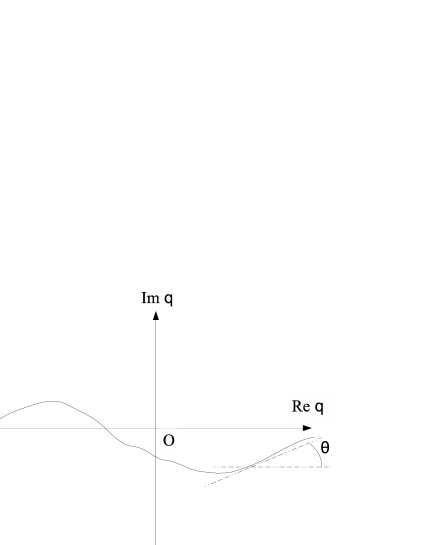
Figure 1: Example of a permitted path $C$

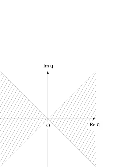
Figure 2: Domain of the delta function

Next, we extend the delta function to complex $\epsilon$, and consider

$$\delta_{c}^{\epsilon}(aq) = \sqrt{\frac{1}{4\pi\epsilon}}e^{-\frac{1}{4\epsilon}a^{2}q^{2}}$$ (11)

for a non-zero complex $a$. We express $\epsilon$, $q$, and $a$ as $\epsilon=r_{\epsilon}e^{i\theta_{\epsilon}}$, $q=r_{q}e^{i\theta_{q}}$, and $a=r_{a}e^{i\theta_{a}}$. The convergence condition of $\delta_{c}^{\epsilon}(aq)$: $\text{Re}\left(\frac{a^{2}q^{2}}{\epsilon}\right)>0$ is expressed as

$$-\frac{\pi}{4}+\frac{1}{2}(\theta_{\epsilon}-2\theta_{a})<\theta_{q}<\frac{\pi}{4}+\frac{1}{2}(\theta_{\epsilon}-2\theta_{a}),$$ (12)

$$\frac{3}{4}\pi+\frac{1}{2}(\theta_{\epsilon}-2\theta_{a})<\theta_{q}<\frac{5}{4}\pi+\frac{1}{2}(\theta_{\epsilon}-2\theta_{a}).$$ (13)

For $q$, $\epsilon$, and $a$ such that Eqs.(12) and (13) are satisfied, $\delta_{c}^{\epsilon}(aq)$ behaves well as a delta function of $aq$, and we obtain the relation

$$\delta_{c}^{\epsilon}(aq)=\frac{\text{sign}(\text{Re}~{}a)}{a}\delta_{c}^{\frac{\epsilon}{a^{2}}}(q),$$ (14)

where we have introduced

$$\text{sign}(\text{Re}a)\equiv\left\{\begin{array}[]{cc}1&\text{for}~{}\text{Re}a>0,\\ -1&\text{for}~{}\text{Re}a<0.\\ \end{array}\right.$$ (17)

2.3 New devices to handle complex parameters

To keep the analyticity in dynamical variables of FPI such as $q$ and $p$, we define a modified set of a complex conjugate, real and imaginary parts, bras, and Hermitian conjugates.

2.3.1 Modified complex conjugate $*_{\{\}}$

We define a modified complex conjugate for a function of $n$ parameters $f(\{a_{i}\}_{i=1,\ldots,n})$ by

$$f(\{a_{i}\}_{i=1,\ldots,n})^{*_{\{a_{i}|i\in A\}}}=f^{*}(\{a_{i}\}_{i\in A},\{a_{i}^{*}\}_{i\not\in A}),$$ (18)

where $A$ denotes the set of indices attached to the parameters in which we keep the analyticity, and $*$ on $f$ acts on the coefficients included in $f$. For example, the complex conjugate $*_{q,p}$ of a function $f(q,p)=aq^{2}+bp^{2}$ is written as $f(q,p)^{*_{q,p}}=a^{*}q^{2}+b^{*}p^{2}$. The analyticity is kept in both $q$ and $p$. For simplicity we express the modified complex conjugate as $*_{\{\}}$, where $\{\}$ is a symbolic expression for a set of parameters in which we keep the analyticity.

2.3.2 Modified real and imaginary parts $\text{Re}_{\{\}}$, $\text{Im}_{\{\}}$

We define the modified real and imaginary parts by using $*_{\{\}}$. We decompose some complex function $f$ as

$$f=\text{Re}_{\{\}}f+i\text{Im}_{\{\}}f,$$ (19)

where $\text{Re}_{\{\}}f$ and $\text{Im}_{\{\}}f$ are the “$\{\}$-real” and “$\{\}$-imaginary” parts of $f$ defined by

$$\text{Re}_{\{\}}f\equiv\frac{f+f^{*_{\{\}}}}{2},$$ (20)

$$\text{Im}_{\{\}}f\equiv\frac{f-f^{*_{\{\}}}}{2i}.$$ (21)

For example, for $f=kq^{2}$, the $q$-real and $q$-imaginary parts of $f$ are expressed as $\text{Re}_{q}f=\text{Re}(k)q^{2}$ and $\text{Im}_{q}f=\text{Im}(k)q^{2}$, respectively. In particular, if $f$ satisfies $f^{*_{\{\}}}=f$, we say $f$ is $\{\}$-real, while if $f$ obeys $f^{*_{\{\}}}=-f$, $f$ is purely $\{\}$-imaginary.

2.3.3 Modified bras ${}_{m}\langle~{}|$ and ${}_{\{\}}\langle~{}|$, and modified Hermitian conjugate ${\dagger}_{\{\}}$

For some state $|\lambda\rangle$ with some complex parameter $\lambda$, we define a modified bra ${}_{m}\langle\lambda|$ by

$${}_{m}\langle\lambda|\equiv\langle\lambda^{*}|$$ (22)

so that it preserves the analyticity in $\lambda$. In the special case of $\lambda$ being real it becomes a normal bra. In addition we define a slightly generalized modified bra ${}_{\{\}}\langle~{}|$ and a modified Hermitian conjugate ${\dagger}_{\{\}}$ of a ket. For example, ${}_{u,v}\langle u|={}_{u}\langle u|={}_{m}\langle u|$, $(|u\rangle)^{{\dagger}_{u,v}}=(|u\rangle)^{{\dagger}_{u}}={}_{m}\langle u|$. We express the Hermitian conjugate ${\dagger}_{\{\}}$ of a ket symbolically as $(|~{}\rangle)^{{\dagger}_{\{\}}}={}_{\{\}}\langle~{}|$. Also, we write the Hermitian conjugate ${\dagger}_{\{\}}$ of a bra as $({}_{\{\}}\langle~{}|)^{{\dagger}_{\{\}}}=|~{}\rangle$. Hence, for a matrix element we have the relation ${}_{\{\}}\langle u|A|v\rangle^{*_{\{\}}}={}_{\{\}}\langle v|A^{\dagger}|u\rangle$.

2.4 Properties of $\hat{q}_{\mathrm{new}}$, $\hat{p}_{\mathrm{new}}$, $|q\rangle_{\mathrm{new}}$, and $|p\rangle_{\mathrm{new}}$

The states $|q\rangle_{\mathrm{new}}$ and $|p\rangle_{\mathrm{new}}$ are normalized so that they satisfy the following relations:

$${}_{m}\langle_{\mathrm{new}}~{}q^{\prime}|q\rangle_{\mathrm{new}} = \delta_{c}^{\epsilon_{1}}(q^{\prime}-q),$$ (23)

$${}_{m}\langle_{\mathrm{new}}~{}p^{\prime}|p\rangle_{\mathrm{new}} = \delta_{c}^{\epsilon^{\prime}_{1}}(p^{\prime}-p),$$ (24)

where $\epsilon_{1}$ and $\epsilon^{\prime}_{1}$ are given by

$$\epsilon_{1} \equiv \frac{\hbar\epsilon}{1-\epsilon\epsilon^{\prime}},$$ (25)

$$\epsilon^{\prime}_{1} \equiv \frac{\hbar\epsilon^{\prime}}{1-\epsilon\epsilon^{\prime}}.$$ (26)

We take $\epsilon$ and $\epsilon^{\prime}$ sufficiently small, for which the delta functions converge for complex $q$, $q^{\prime}$, $p$, and $p^{\prime}$ satisfying the conditions $L(q-q^{\prime})>0$ and $L(p-p^{\prime})>0$, where $L$ is given in Eq.(10). These conditions are satisfied only when $q$ and $q^{\prime}$ or $p$ and $p^{\prime}$ are on the same paths respectively. For small $\epsilon$ and $\epsilon^{\prime}$, Eqs.(23) and (24) represent the orthogonality relations for $|q\rangle_{\mathrm{new}}$ and $|p\rangle_{\mathrm{new}}$, and we have the following relations:

$$\int_{C}dq|q\rangle_{\mathrm{new}}~{}{}_{m}\langle_{\mathrm{new}}q|\simeq 1,$$ (27)

$$\int_{C}dp|p\rangle_{\mathrm{new}}~{}{}_{m}\langle_{\mathrm{new}}p|\simeq 1,$$ (28)

$$\hat{p}_{\mathrm{new}}^{\dagger}|q\rangle_{\mathrm{new}}\simeq i\hbar\frac{\partial}{\partial q}|q\rangle_{\mathrm{new}},$$ (29)

$$\hat{q}_{\mathrm{new}}^{\dagger}|p\rangle_{\mathrm{new}}\simeq\frac{\hbar}{i}\frac{\partial}{\partial p}|p\rangle_{\mathrm{new}},$$ (30)

$${}_{m}\langle_{\mathrm{new}}~{}q|p\rangle_{\mathrm{new}}\simeq\frac{1}{\sqrt{2\pi\hbar}}\exp\left(\frac{i}{\hbar}pq\right).$$ (31)

Thus, $\hat{q}_{\mathrm{new}}^{\dagger}$, $\hat{p}_{\mathrm{new}}^{\dagger}$, $|q\rangle_{\mathrm{new}}$, and $|p\rangle_{\mathrm{new}}$ with complex $q$ and $p$ obey the same relations as $\hat{q}$, $\hat{p}$, $|q\rangle$, and $|p\rangle$ with real $q$ and $p$. In the $\epsilon\rightarrow 0$ and $\epsilon^{\prime}\rightarrow 0$ limits, $\delta_{c}^{\epsilon_{1}}(q^{\prime}-q)$, $\delta_{c}^{\epsilon^{\prime}_{1}}(p^{\prime}-p)$, and $\exp\left(\frac{i}{\hbar}pq\right)$ in Eqs.(23), (24), and (31) are well defined as distributions of the class ${\cal D}$. For real $q^{\prime}$ and $p^{\prime}$, $|q^{\prime}\rangle_{\mathrm{new}}$ and $|p^{\prime}\rangle_{\mathrm{new}}$ become $|q^{\prime}\rangle$ and $|p^{\prime}\rangle$ respectively; also, $\hat{q}_{\mathrm{new}}^{\dagger}$ and $\hat{p}_{\mathrm{new}}^{\dagger}$ behave like $\hat{q}$ and $\hat{p}$ respectively.

3 Harmonic oscillator model and phase diagram in $m$ and $\omega$

In this section, after reviewing the future-included theory, we define our harmonic oscillator model in the CAT and present the phase diagram.

3.1 Harmonic oscillator Hamiltonian in the future-included theory

3.1.1 Future-included theory

The future-included theory[1, 26, 27] is described by using the future state $|B(T_{B})\rangle$ at the final time $T_{B}$ and the past state $|A(T_{A})\rangle$ at the initial time $T_{A}$. For a given non-normal Hamiltonian $\hat{H}$, $|A(t)\rangle$ and $|B(t)\rangle$ obey the Schrödinger equations

$$i\hbar\frac{d}{dt}|A(t)\rangle=\hat{H}|A(t)\rangle,$$ (32)

$$i\hbar\frac{d}{dt}|B(t)\rangle={\hat{H}}^{{\dagger}}|B(t)\rangle,$$ (33)

and are expressed as

$$|A(t)\rangle = e^{-\frac{i}{\hbar}\hat{H}(t-T_{A})}|A(T_{A})\rangle,$$ (34)

$$|B(t)\rangle = e^{-\frac{i}{\hbar}\hat{H}^{\dagger}(t-T_{B})}|B(T_{B})\rangle.$$ (35)

In Refs.[26, 27], we investigated the normalized matrix element $\langle\hat{\cal O}\rangle^{BA}\equiv\frac{\langle B(t)|\hat{\cal O}|A(t)\rangle}{\langle B(t)|A(t)\rangle}$, which is called the weak value[24, 25] in the RAT, and found that if we regard $\langle\hat{\cal O}\rangle^{BA}$ as an expectation value in the future-included theory, then we obtain the Heisenberg equation, Ehrenfest’s theorem, and a conserved probability current density. In fact, since $\langle\hat{\cal O}\rangle^{BA}$ obeys

$$\frac{d}{dt}\langle\hat{\cal O}\rangle^{BA} = \langle\frac{i}{\hbar}[\hat{H},\hat{\cal O}]\rangle^{BA}$$ (36)

for a general Hamiltonian

$$\hat{H}=\frac{1}{2m}\hat{p}_{\mathrm{new}}^{2}+V(\hat{q}_{\mathrm{new}}),$$ (37)

where $V$ is a general potential defined by $V(q)=\sum_{n=2}^{\infty}b_{n}q^{n}$, we obtain

$$\frac{d}{dt}\langle\hat{q}_{\mathrm{new}}\rangle^{BA}=\frac{1}{m}\langle\hat{p}_{\mathrm{new}}\rangle^{BA},$$ (38)

$$\frac{d}{dt}\langle\hat{p}_{\mathrm{new}}\rangle^{BA}=-\langle V^{\prime}(\hat{q}_{\mathrm{new}})\rangle^{BA},$$ (39)

and Ehrenfest’s theorem, $m\frac{d^{2}}{dt^{2}}\langle\hat{q}_{\mathrm{new}}\rangle^{BA}=-\langle V^{\prime}(\hat{q}_{\mathrm{new}})\rangle^{BA}$. Thus, $\langle\hat{\cal O}\rangle^{BA}$ provides the time development of the saddle point for $\exp(\frac{i}{\hbar}S)$, and seems to have the role of an expectation value in the future-included theory. In addition, let us introduce a probability density $\rho$ by

$$\rho\equiv\frac{\psi_{B}(q)^{*_{q}}\psi_{A}(q)}{\langle B|A\rangle}=\frac{\langle B|q\rangle_{\mathrm{new}}~{}{}_{m}\langle_{\mathrm{new}}~{}q|A\rangle}{\langle B|A\rangle},$$ (40)

which satisfies $\int_{C}dq\rho=1$, where $C$ is an arbitrary contour running from $-\infty$ to $\infty$ in the complex $q$-plane. Then we can construct a conserved probability current density $j$ by

$$j(q,t)\equiv\frac{\frac{i\hbar}{2m}\left(\frac{\partial\tilde{\psi}_{B}^{*_{q}}}{\partial q}\psi_{A}-\tilde{\psi}_{B}^{*_{q}}\frac{\partial\psi_{A}}{\partial q}\right)}{\langle B|A\rangle},$$ (41)

which obeys the continuity equation $\frac{\partial\rho}{\partial t}+\frac{\partial}{\partial q}j(q,t)=0$. Therefore, probability interpretation seems to work formally with this $\rho$.

As for the Lagrangian, in Ref. [21], starting from the Hamiltonian given in Eq.(37), we obtained via the FPI the Lagrangian $L(q,\dot{q})=\frac{1}{2}m\dot{q}^{2}-\sum_{n=2}^{\infty}b_{n}q^{n}$, and vice versa. In addition, we derived via the FPI the momentum relation

$$p(t)=m\frac{d}{dt}q(t).$$ (42)

We note that this is not the case in the future-not-included CAT. Indeed, we showed in Ref. [22] that in the future-not-included CAT the Lagrangian and momentum relation are given by $L_{\text{eff}}(\dot{q},q)=\frac{1}{2}m_{\text{eff}}~{}\dot{q}^{2}-\sum_{n=2}^{\infty}\text{Re}b_{n}~{}q^{n}$ and $p=m_{\mathrm{eff}}\dot{q}$, where $m_{\text{eff}}\equiv m_{\mathrm{R}}+\frac{m_{\mathrm{I}}^{2}}{m_{\mathrm{R}}}$. Since Eq.(38) is consistent with Eq.(42), Eq.(42) is confirmed to be the momentum relation in the future-included theory.

3.1.2 Harmonic oscillator Hamiltonian

Utilizing $\hat{q}_{\mathrm{new}}$ and $\hat{p}_{\mathrm{new}}$ given in Eqs.(5) and (6), we define our harmonic oscillator Hamiltonian $\hat{H}$ by

$$\hat{H}\equiv\frac{1}{2m}\hat{p}_{\mathrm{new}}^{2}+V(\hat{q}_{\mathrm{new}}),$$ (43)

$$V(\hat{q}_{\mathrm{new}})=\frac{1}{2}m\omega^{2}\hat{q}_{\mathrm{new}}^{2},$$ (44)

where both mass $m$ and angular frequency $\omega$ are complex, and decomposed as follows:

$$m=m_{\mathrm{R}}+im_{\mathrm{I}}=r_{m}e^{i\theta_{m}},$$ (45)

$$\omega=\omega_{\mathrm{R}}+i\omega_{\mathrm{I}}=r_{\omega}e^{i\theta_{\omega}},$$ (46)

where $m_{\mathrm{R}}$, $\omega_{\mathrm{R}}$, $m_{\mathrm{I}}$, and $\omega_{\mathrm{I}}$ are the real and imaginary parts of $m$ and $\omega$, and $r_{m}$, $r_{\omega}$, $\theta_{m}$, and $\theta_{\omega}$ are the absolute values and arguments of $m$ and $\omega$, respectively. This Hamiltonian depends on $\epsilon$ and $\epsilon^{\prime}$ via $\hat{q}_{\mathrm{new}}$ and $\hat{p}_{\mathrm{new}}$. For our later convenience, let us introduce another Hamiltonian that is independent of $\epsilon$ and $\epsilon^{\prime}$,

$$\hat{H}_{\epsilon=\epsilon^{\prime}=0}\equiv\frac{1}{2m}\hat{p}^{2}+\frac{1}{2}m\omega^{2}\hat{q}^{2},$$ (47)

by taking the limits $\epsilon\rightarrow 0$ and $\epsilon^{\prime}\rightarrow 0$, or replacing $\hat{q}_{\mathrm{new}}$ and $\hat{p}_{\mathrm{new}}$ with $\hat{q}$ and $\hat{p}$ in $\hat{H}$. Utilizing the fact obtained in Ref. [21], we find that the Lagrangian is simply given by

$$L(q,\dot{q}) = \frac{1}{2}m\dot{q}^{2}-V(q),$$ (48)

$$V(q) = \frac{1}{2}m\omega^{2}q^{2}.$$ (49)

The potential $V$ is decomposed as

$$V = V_{\mathrm{R}}+iV_{\mathrm{I}},$$ (50)

$$V_{\mathrm{R}} \equiv \text{Re}_{q}V=\text{Re}\left(\frac{m\omega^{2}}{2}\right)q^{2},$$ (51)

$$V_{\mathrm{I}} \equiv \text{Im}_{q}V=\text{Im}\left(\frac{m\omega^{2}}{2}\right)q^{2},$$ (52)

where $\text{Re}_{q}$ and $\text{Im}_{q}$ are introduced in Eqs.(20) and (21).

We consider the functional integral $\int_{C}{\cal D}q~{}\psi_{B}^{*}\psi_{A}e^{\frac{i}{\hbar}\int L(q,\dot{q})dt}$, and suppose that the asymptotic values of dynamical variables such as $q$ and $p$ are on the real axis. The path $C$ denotes an arbitrary path running from $-\infty$ to $\infty$ in the complex plane for each moment of time $t$, and we can deform it as long as the integrand keeps the analyticity in $q$ and $p$. To prevent the kinetic term in the integrand from blowing up for $\dot{q}\rightarrow\pm\infty$ along the real axis, we impose on $m$ the condition

$$m_{\mathrm{I}}\geq 0.$$ (53)

In addition, to ensure the convergence of the functional integral, we need the following condition on the potential:

$$\text{Im}(m\omega^{2})\leq 0.$$ (54)

Then, since $m\omega$ and $m\omega^{2}$ are written as

$$m\omega\equiv re^{i\theta}=r_{m}r_{\omega}e^{i(\theta_{m}+\theta_{\omega})},$$ (55)

$$m\omega^{2}=r_{m}r_{\omega}^{2}e^{i(\theta_{m}+2\theta_{\omega})},$$ (56)

the two conditions in Eqs.(53) and (54) are expressed in terms of $\theta_{m}$ and $\theta_{\omega}$ as

$$0\leq\theta_{m}\leq\pi,$$ (57)

$$-\pi\leq\theta_{m}+2\theta_{\omega}\leq 0\quad\leftrightarrow\quad-\frac{\theta_{m}}{2}-\frac{\pi}{2}\leq\theta_{\omega}\leq-\frac{\theta_{m}}{2},$$ (58)

respectively.

3.2 Study of the phase diagram

In this subsection we analyze the phase diagram in the $(\theta_{m},\theta_{\omega})$ plane. We will see that, according to the values of $\theta_{m}$ and $\theta_{\omega}$, our harmonic oscillator model includes several different theories. Indeed, the value of $\theta_{m}$ classifies the model into the usual time theory (UTT), imaginary time theory (ITT) and flipped time theory (FTT). Also, according to the value of $\theta_{\omega}$, not only a harmonic oscillator (HO) but also an inverted harmonic oscillator (IHO) is described.

Using Eq.(56), let us express $V_{\mathrm{R}}$ and $V_{\mathrm{I}}$ given in Eqs.(51) and (52) as

$$V_{\mathrm{R}} = \frac{q^{2}}{2}r_{m}r_{\omega}^{2}\cos(\theta_{m}+2\theta_{\omega}),$$ (59)

$$V_{\mathrm{I}} = \frac{q^{2}}{2}r_{m}r_{\omega}^{2}\sin(\theta_{m}+2\theta_{\omega}).$$ (60)

Then, according to the signs of $V_{\mathrm{R}}$ and $V_{\mathrm{I}}$, the permitted region of $\theta_{\omega}$ by the condition in Eq.(58) can be classified into the following five regions:

1. For $\theta_{\omega}=-\frac{\theta_{m}}{2}\quad\Leftrightarrow\quad\theta_{m}+2\theta_{\omega}=0$:

   $V_{\mathrm{R}}>0$, $V_{\mathrm{I}}=0$.

2. For $-\frac{\theta_{m}}{2}-\frac{\pi}{4}<\theta_{\omega}<-\frac{\theta_{m}}{2}\quad\Leftrightarrow\quad-\frac{\pi}{2}<\theta_{m}+2\theta_{\omega}<0$:

   $V_{\mathrm{R}}>0$, $V_{\mathrm{I}}<0$.

3. For $\theta_{\omega}=-\frac{\theta_{m}}{2}-\frac{\pi}{4}\quad\Leftrightarrow\quad\theta_{m}+2\theta_{\omega}=-\frac{\pi}{2}$:

   $V_{\mathrm{R}}=0$, $V_{\mathrm{I}}<0$.

4. For $-\frac{\theta_{m}}{2}-\frac{\pi}{2}<\theta_{\omega}<-\frac{\theta_{m}}{2}-\frac{\pi}{4}\quad\Leftrightarrow\quad-\pi<\theta_{m}+2\theta_{\omega}<-\frac{\pi}{2}$:

   $V_{\mathrm{R}}<0$, $V_{\mathrm{I}}<0$.

5. For $\theta_{\omega}=-\frac{\theta_{m}}{2}-\frac{\pi}{2}\quad\Leftrightarrow\quad\theta_{m}+2\theta_{\omega}=-\pi$:

   $V_{\mathrm{R}}<0$, $V_{\mathrm{I}}=0$.

Later, using the different condition in Eq.(57), we investigate these regions in more detail according to the value of $\theta_{m}$.

3.2.1 Our principle of interpretation of various quantities in the CAT

We shall explain our interpretation of various quantities in the CAT. We allow both mass $m$ and angular frequency $\omega$ to be complex, so negative numbers are naturally included. Since we have a much larger class of theories, there can only be a priori less chance that we obtain just what we find in nature. Some possible outcomes will simply disagree with some of our experiences. We have to choose the parameters appropriately. We then divide the possibilities for the sign of the real part of $m$ called $m_{\mathrm{R}}$ to classify the theories. We think that the real part of (non-relativistic) mass should be positive in a sensible theory. One possible strategy would be to declare that there is an empirical law that $m_{\mathrm{R}}$ shall be positive. Another one would be to introduce some transformation to change the mass into a new mass so that its real part becomes positive. Based on this way of thinking, we define a new mass by

$$m_{\mathrm{new}}\equiv am,$$ (61)

where $a$, whose magnitude is $1$, is properly chosen so that $\text{Re}~{}m_{\mathrm{new}}>0$. Since $\theta_{m}=\arg m$ is restricted by the condition in Eq.(57), $a$ is chosen according to the sign of $m_{\mathrm{R}}$, as shown later.

Next we introduce new times $t_{\mathrm{new}}$ and $T_{A}^{\mathrm{new}}$, and a new angular frequency $\omega_{\mathrm{new}}$ by demanding the relation

$$\exp\left[-\frac{i}{\hbar}\hat{H}(t-T_{A})\right] = \exp\left[-\frac{i}{\hbar}\hat{H}_{\mathrm{new}}(t_{\mathrm{new}}-T_{A}^{\mathrm{new}})\right]$$ (62)

for the Hamiltonian $\hat{H}$ given in Eqs.(43) and (44), and a new Hamiltonian $\hat{H}_{\mathrm{new}}$ defined by

$$\hat{H}_{\mathrm{new}} \equiv \frac{\hat{p}_{\mathrm{new}}^{2}}{2m_{\mathrm{new}}}+\frac{1}{2}m_{\mathrm{new}}\omega_{\mathrm{new}}^{2}\hat{q}_{\mathrm{new}}^{2}=\frac{1}{a}\hat{H}.$$ (63)

Comparing the free parts of $\hat{H}$ and $\hat{H}_{\mathrm{new}}$ on both sides of Eq.(62), we define

$$t_{\mathrm{new}}\equiv\frac{m_{\mathrm{new}}}{m}t=at,$$ (64)

and $T_{A}^{\mathrm{new}}\equiv\frac{m_{\mathrm{new}}}{m}T_{A}=aT_{A}$. Similarly, we define $T_{B}^{\mathrm{new}}\equiv aT_{B}$. In addition, we introduce a new pair of coordinate and momentum, $q_{\mathrm{new}}$ and $p_{\mathrm{new}}$, by

$$q_{\mathrm{new}}(t_{\mathrm{new}}) \equiv q(t),$$ (65)

$$p_{\mathrm{new}}(t_{\mathrm{new}}) \equiv p(t).$$ (66)

Using Eqs.(64)-(66), we can rewrite the momentum relation given in Eq.(42) in terms of the new variables as $p_{\mathrm{new}}(t_{\mathrm{new}})=m_{\mathrm{new}}\frac{d}{dt_{\mathrm{new}}}q_{\mathrm{new}}(t_{\mathrm{new}})$. Next we compare the potential terms of $\hat{H}$ and $\hat{H}_{\mathrm{new}}$ on both sides of Eq.(62). Then we might feel like defining $\omega_{\mathrm{new}}=\pm\frac{1}{a}\omega$, where we encounter an indefiniteness for the sign of $\omega_{\mathrm{new}}$. However, since the expression of Eq.(63) suggests a new energy $E_{\mathrm{new}}\equiv\frac{1}{a}\lambda_{n}$, if we suppose that we can obtain an energy eigenvalue $\lambda_{n}\equiv\hbar\omega\left(n+\frac{1}{2}\right)$ for $\hat{H}$, we are led to defining $\omega_{\mathrm{new}}$ with a definite sign by

$$\omega_{\mathrm{new}}\equiv\frac{1}{a}\omega,$$ (67)

so that $E_{\mathrm{new}}$ is expressed as $E_{\mathrm{new}}=\hbar\omega_{\mathrm{new}}\left(n+\frac{1}{2}\right)$. Equation (67) is also given by demanding the relation $\omega t=\omega_{\mathrm{new}}t_{\mathrm{new}}$.

According to the sign of $m_{\mathrm{R}}$, we determine $m_{\mathrm{new}}$, $\omega_{\mathrm{new}}$, and $t_{\mathrm{new}}$ as follows:

1. For $0\leq\theta_{m}<\frac{\pi}{2}$:

   Since $m_{\mathrm{R}}>0$, we choose $a=1$, i.e. $m_{\mathrm{new}}=m$, $\omega_{\mathrm{new}}=\omega$, and $t_{\mathrm{new}}=t$.

2. For $\theta_{m}=\frac{\pi}{2}$:

   Since $m_{\mathrm{R}}=0$, we choose $a=-i$, i.e. $m_{\mathrm{new}}=-im$, $\omega_{\mathrm{new}}=i\omega$, and $t_{\mathrm{new}}=-it$.

3. For $\frac{\pi}{2}<\theta_{m}\leq\pi$:

   Since $m_{\mathrm{R}}<0$, we choose $a=-1$, i.e. $m_{\mathrm{new}}=-m$, $\omega_{\mathrm{new}}=-\omega$, and $t_{\mathrm{new}}=-t$.

Unless one transforms the negativity of $m_{\mathrm{R}}$ away, cases 2 and 3 would be forbidden by the empirical law that $m_{\mathrm{R}}$ shall be positive.

3.2.2 The phase diagram

Based on the strategy given in Sect. 3.2.1, we can classify our harmonic oscillator model into several theories. We have presented such an explicit study in Appendix A. Thus, the phase diagram of the harmonic oscillator specified by Eqs.(57) and (58) is drawn in Fig.3.

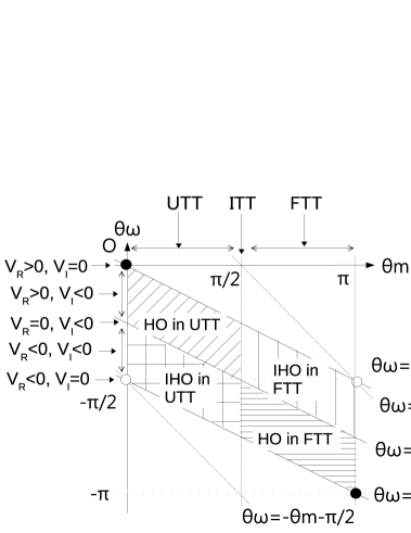
Figure 3: The phase diagram of the harmonic oscillator defined with complex $m$ and $\omega$. Here $\theta_{m}=\arg m$ and $\theta_{\omega}=\arg\omega$, as defined in Eqs.(45) and (46). The special cases contained in the RAT are at the four corners of the allowed parallelogram region. A usual harmonic oscillator model having positive energy is defined at the upper left corner.

4 Two-basis formalism

In this section we develop our two-basis formalism of eigenvectors for the harmonic oscillator Hamiltonians $\hat{H}$ and $\hat{H}^{\dagger}$.

4.1 Annihilation and creation operators

We define two annihilation operators, $\hat{a}_{1}$ and $\hat{a}_{2}$, and creation operators, $\hat{a}_{1}^{\dagger}$ and $\hat{a}_{2}^{\dagger}$, by their Hermitian conjugates as follows:

$$\hat{a}_{1}=\sqrt{\frac{m\omega}{2\hbar}}\left(\hat{q}_{\mathrm{new}}+\frac{i\hat{p}_{\mathrm{new}}}{m\omega}\right),$$ (68)

$$\hat{a}_{2}=\sqrt{\frac{m^{*}\omega^{*}}{2\hbar}}\left(\hat{q}_{\mathrm{new}}^{\dagger}+\frac{i\hat{p}_{\mathrm{new}}^{\dagger}}{m^{*}\omega^{*}}\right),$$ (69)

$$\hat{a}_{2}^{\dagger}=\sqrt{\frac{m\omega}{2\hbar}}\left(\hat{q}_{\mathrm{new}}-\frac{i\hat{p}_{\mathrm{new}}}{m\omega}\right),$$ (70)

$$\hat{a}_{1}^{\dagger}=\sqrt{\frac{m^{*}\omega^{*}}{2\hbar}}\left(\hat{q}_{\mathrm{new}}^{\dagger}-\frac{i\hat{p}_{\mathrm{new}}^{\dagger}}{m^{*}\omega^{*}}\right).$$ (71)

Equations (68) and (70) provide $\hat{q}_{\mathrm{new}}$ and $\hat{p}_{\mathrm{new}}$ in terms of $\hat{a}_{1}$ and $\hat{a}_{2}^{\dagger}$ as

$$\hat{q}_{\mathrm{new}} = \sqrt{\frac{\hbar}{2m\omega}}(\hat{a}_{1}+\hat{a}_{2}^{\dagger}),$$ (72)

$$\hat{p}_{\mathrm{new}} = -i\sqrt{\frac{\hbar m\omega}{2}}(\hat{a}_{1}-\hat{a}_{2}^{\dagger}).$$ (73)

Then, the commutation relation $[\hat{q}_{\mathrm{new}},\hat{p}_{\mathrm{new}}]=i\hbar$ is written as

$$[\hat{a}_{1},\hat{a}_{2}^{\dagger}]=1,$$ (74)

and the Hamiltonian $\hat{H}$ in Eq.(43) and its Hermitian conjugate $\hat{H}^{\dagger}$ are expressed in terms of $\hat{a}_{1}$ and $\hat{a}_{2}^{\dagger}$ as

$$\hat{H} = \hbar\omega\left(\hat{a}_{2}^{\dagger}\hat{a}_{1}+\frac{1}{2}\right),$$ (75)

$$\hat{H}^{\dagger} = \hbar\omega^{*}\left(\hat{a}_{1}^{\dagger}\hat{a}_{2}+\frac{1}{2}\right).$$ (76)

We define two ground states $|0\rangle_{1}$ and $|0\rangle_{2}$ up to the normalization by

$$\hat{a}_{1}|0\rangle_{1}=0,$$ (77)

$$\hat{a}_{2}|0\rangle_{2}=0,$$ (78)

and excited states $|n\rangle_{1}$ and $|n\rangle_{2}$ for positive integer $n$ up to the normalization as $|n\rangle_{1}\propto(\hat{a}_{2}^{\dagger})^{n}|0\rangle_{1}$ and $|n\rangle_{2}\propto(\hat{a}_{1}^{\dagger})^{n}|0\rangle_{2}$. In addition, we introduce number operators $\hat{n}_{1}$ and $\hat{n}_{2}$ by

$$\hat{n}_{1}=\hat{a}_{2}^{\dagger}\hat{a}_{1},$$ (79)

$$\hat{n}_{2}=\hat{a}_{1}^{\dagger}\hat{a}_{2}=\hat{n}_{1}^{\dagger}.$$ (80)

Then they obey $\hat{n}_{1}|n\rangle_{1}=n|n\rangle_{1}$ and $\hat{n}_{2}|n\rangle_{2}=n|n\rangle_{2}$, and $\hat{H}$ and $\hat{H}^{\dagger}$ are expressed as

$$\hat{H}=\hbar\omega\left(\hat{n}_{1}+\frac{1}{2}\right),$$ (81)

$$\hat{H}^{\dagger}=\hbar\omega^{*}\left(\hat{n}_{2}+\frac{1}{2}\right).$$ (82)

We see that $|n\rangle_{1}$ and $|n\rangle_{2}$ are eigenstates of $\hat{H}$ and $\hat{H}^{\dagger}$,

$$\hat{H}|n\rangle_{1}=\hbar\omega\left(n+\frac{1}{2}\right)|n\rangle_{1},$$ (83)

$$\hat{H}^{\dagger}|n\rangle_{2}=\hbar\omega^{*}\left(n+\frac{1}{2}\right)|n\rangle_{2},$$ (84)

so, in particular, $\hat{H}$ has the following eigenvalue for $|n\rangle_{1}$:

$$\lambda_{n}=\hbar\omega\left(n+\frac{1}{2}\right).$$ (85)

Here we note that $|n\rangle_{1}$ and $|n\rangle_{2}$ are not orthogonal eigenstates; ${}_{1}\langle m|n\rangle_{1}$ and ${}_{2}\langle m|n\rangle_{2}$ are not proportional to $\delta_{mn}$, since $\hat{H}$ and $\hat{H}^{\dagger}$ are not Hermitian. Though these eigenstates $|n\rangle_{1}$ and $|n\rangle_{2}$ are technically somewhat hard to normalize, we can construct rather easily two series of eigenstates that are not genuinely normalized but fixed by a convention that makes the algebra of $\hat{a}_{2}^{\dagger}$ and $\hat{a}_{1}$ work very elegantly like in the RAT case.

4.2 Normalization of $|n\rangle_{1}$ and $|n\rangle_{2}$

In this subsection we shall discuss how we normalize the series of Hilbert vectors $|n\rangle_{1}$ and $|n\rangle_{2}$. There could be a number of ways of normalizing them. We first explain them.

1) We can imagine the special set of $|n\rangle_{1}$ by a naive analytical continuation of the $q$-representation of the normalized state in the RAT, $|n\rangle=\frac{1}{\sqrt{n!}}(\hat{a}^{\dagger})^{n}|0\rangle$, to complex $m\omega$ for small $\epsilon$ and $\epsilon^{\prime}$:

$${}_{m}\langle_{\mathrm{new}}~{}q|n\rangle_{1}\simeq\left(\frac{m\omega}{\pi\hbar}\right)^{\frac{1}{4}}\frac{1}{\sqrt{n!}}\left(\frac{1}{\sqrt{2}}\right)^{n}H_{n}\left(\sqrt{\frac{m\omega}{\hbar}}q\right)\exp\left(-\frac{m\omega}{2\hbar}q^{2}\right),$$ (86)

where on the left-hand side we have used a modified bra for complex $q$, and on the right-hand side $H_{n}(x)$ is the $n$th Hermite polynomial, $H_{n}(x)=\exp\left(\frac{1}{2}x^{2}\right)\left(x-\frac{d}{dx}\right)^{n}\exp\left(-\frac{1}{2}x^{2}\right)$. In particular, ${}_{m}\langle_{\mathrm{new}}~{}q|0\rangle_{1}$ is expressed as

$${}_{m}\langle_{\mathrm{new}}~{}q|0\rangle_{1}\simeq\left(\frac{m\omega}{\pi\hbar}\right)^{\frac{1}{4}}\exp\left(-\frac{m\omega}{2\hbar}q^{2}\right).$$ (87)

Replacing $m\omega$ with $m^{*}\omega^{*}$ in the RAT state $|n\rangle$ and then analytically continuing in $m^{*}\omega^{*}$, we obtain the set $|n\rangle_{2}$ for small $\epsilon$ and $\epsilon^{\prime}$:

$${}_{m}\langle_{\mathrm{new}}~{}q|n\rangle_{2} \simeq \left(\frac{m^{*}\omega^{*}}{\pi\hbar}\right)^{\frac{1}{4}}\frac{1}{\sqrt{n!}}\left(\frac{1}{\sqrt{2}}\right)^{n}H_{n}\left(\sqrt{\frac{m^{*}\omega^{*}}{\hbar}}q\right)\exp\left(-\frac{m^{*}\omega^{*}}{2\hbar}q^{2}\right).$$ (88)

Let us consider the correction to complex $q$ for the $n$th Hermite polynomial $H_{n}(q)$. $H_{n}(q)$ is a smooth $q$-wave function for small $n$, but not so for large $n$, for which it oscillates considerably. Comparing the expressions for the Hamiltonian $\hat{H}$ in Eqs.(43) and (83), we see that $q$ and $p$ classically go up in proportion to $\sqrt{n}$ for large $n$. Hence, the width of $H_{n}(q)$ is proportional to $\sqrt{n}$. In addition, $H_{n}(q)$ has $n$ zeros. Since the density of zeros is about $\frac{n}{\sqrt{n}}=\sqrt{n}$ per unit length in $q$, the length of each wave contained in $H_{n}(q)$ is about $\frac{1}{\sqrt{n}}$. On the other hand, the correction to complex $q$ is $\epsilon p\sim\epsilon\sqrt{n}$. It is $\epsilon\sqrt{n}/{\frac{1}{\sqrt{n}}}\sim\epsilon n$ relative to the wave length. Therefore, when $\epsilon n>1$ we cannot ignore the $\epsilon p$ term anymore. So the expressions in Eqs.(86) and (88) are valid for $n$ such that $n<\frac{1}{\epsilon}$.

The expression of Eq.(86), which is a function of $m\omega$ but not $m^{*}\omega^{*}$, motivates us to define our $|n\rangle_{1}$ including the factor in front by

$$|n\rangle_{1}\equiv\frac{1}{\sqrt{n!}}(\hat{a}_{2}^{\dagger})^{n}|0\rangle_{1}.$$ (89)

The state $|n\rangle_{1}$ is not normalized in the usual sense. The squared norm of $|n\rangle_{1}$ involves both $m\omega$ and $m^{*}\omega^{*}$, so it is not analytic in $m\omega$. Similarly, we are motivated to define our $|n\rangle_{2}$ by

$$|n\rangle_{2}\equiv\frac{1}{\sqrt{n!}}(\hat{a}_{1}^{\dagger})^{n}|0\rangle_{2}.$$ (90)

2) We could also single out our proposed series of eigenstate $|n\rangle_{1}$ by the requirement of the usual ladder formulas with $\hat{a}_{2}^{\dagger}$ and $\hat{a}_{1}$ replacing $a^{\dagger}$ and $a$ respectively,

$$\hat{a}_{2}^{\dagger}|n\rangle_{1}=\sqrt{n+1}|n+1\rangle_{1},$$ (91)

$$\hat{a}_{1}|n\rangle_{1}=\sqrt{n}|n-1\rangle_{1}.$$ (92)

This algebraic requirement – not involving any norm – specifies the $|n\rangle_{1}$ state even with respect to $n$-dependent scale factors. To consider the set $|n\rangle_{2}$ in the same way, the algebraic requirement in Eqs.(91) and (92) should be replaced with the following ladder equations:

$$\hat{a}_{1}^{\dagger}|n\rangle_{2}=\sqrt{n+1}|n+1\rangle_{2},$$ (93)

$$\hat{a}_{2}|n\rangle_{2}=\sqrt{n}|n-1\rangle_{2}.$$ (94)

In our definitions $\hat{a}_{1}^{\dagger}$ and $\hat{a}_{2}$ are the ladder operators depending on $m^{*}\omega^{*}$, while $\hat{a}_{2}^{\dagger}$ and $\hat{a}_{1}$ used for construction of the $|n\rangle_{1}$ states are the ones depending on $m\omega$.

3) The third possibility is to try to determine both the prefactors of $|n\rangle_{1}$ and $|n\rangle_{2}$ by imposing the condition

$${}_{2}\langle m|n\rangle_{1}=\delta_{mn}$$ (95)

on $|n\rangle_{1}$ and $|m\rangle_{2}$. This condition means that $|m\rangle_{2}$ is regarded as a dual basis of $|n\rangle_{1}$, and also implies the following completeness relation:

$$\sum_{n=0}^{\infty}|n\rangle_{1}~{}{}_{2}\langle n|=1.$$ (96)

If we write $|n\rangle_{1}$ and $|m\rangle_{2}$ as $|n\rangle_{1}=C_{1}(n)(\hat{a}_{2}^{\dagger})^{n}|0\rangle_{1}$ and $|m\rangle_{2}=C_{2}(m)(\hat{a}_{1}^{\dagger})^{m}|0\rangle_{2}$, then Eq.(95) gives only the condition $C_{2}(n)^{*}C_{1}(n)=\frac{1}{n!}$. Choosing $C_{1}(n)$ and $C_{2}(n)$ symmetrically as $C_{1}(n)=C_{2}(n)=\frac{1}{\sqrt{n!}}$ leads to the $|n\rangle_{1}$ of Eq.(89) specified by $1)$ and $2)$, and the analogue for $|n\rangle_{2}$ given in Eq.(90). This procedure $3)$ does not quite fix the normalization of $|n\rangle_{1}$ alone, but needs to be supplemented by $1)$ or $2)$. The condition in Eq.(95) indeed follows from the scale specifications suggested under $1)$ and $2)$, i.e. the analytical continuation and the ladder relation requirements respectively, if they are supplemented by the analogous construction of the $|n\rangle_{2}$ states. We call this “dual normalization”.

Using the above rules $1)$, $2)$, and $3)$, which are consistent with each other, we have specified two series of eigenstates $|n\rangle_{1}$ and $|n\rangle_{2}$ of $\hat{H}$ and $\hat{H}^{\dagger}$ respectively. They formally look like being normalized in the usual sense, but actually only in the sense of the dual normalization by Eq.(95). The two-basis formalism of $|n\rangle_{1}$ and $|m\rangle_{2}$ is our replacement for the usual formalism of $|n\rangle$ in the RAT. Indeed, we first define our ground states $|0\rangle_{1}$ and $|0\rangle_{2}$ by Eqs.(77), (78), and (95), where we choose their normalization factors symmetrically. Second, we define our $|n\rangle_{1}$ and $|n\rangle_{2}$ for $n\geq 1$ by Eqs.(89) and (90). Then we obtain for the overlap ${}_{2}\langle m|n\rangle_{1}$ the same result $\delta_{mn}$ as in the RAT, i.e. Eq.(95), and our states $|n\rangle_{1}$ and $|n\rangle_{2}$ obey the ladder relations given in Eqs.(91), (92), (93), and (94).

The point is that, when we take the bra ${}_{2}\langle m|$ correlated to the ket $|m\rangle_{2}$, we get an expression formally written in terms of $m\omega$, and thus the overlap ${}_{2}\langle m|n\rangle_{1}$ becomes an integral of an expression involving only $m\omega$ to be an analytical continuation of $\langle m|n\rangle$ in $m\omega$, which is well known to give $\delta_{mn}$. For ${}_{2}\langle n|n^{\prime}\rangle_{1}$ we can see this property even by using the concrete expressions of Eqs.(86) and (88) for small $\epsilon$ and $\epsilon^{\prime}$ as follows:

$${}_{2}\langle n|n^{\prime}\rangle_{1} \simeq \int dq~{}{}_{2}\langle n|q\rangle_{\mathrm{new}}~{}{}_{m}\langle_{\mathrm{new}}~{}q|n^{\prime}\rangle_{1}$$ (97)

$$\simeq \frac{1}{\sqrt{n!n^{\prime}!}}\left(\frac{1}{\sqrt{2}}\right)^{n+n^{\prime}}\left(\frac{m\omega}{\pi\hbar}\right)^{\frac{1}{2}}\left(\frac{\hbar}{m\omega}\right)^{\frac{1}{2}}\int dXH_{n}(X)H_{n^{\prime}}(X)\exp(-X^{2})$$

$$= \delta_{nn^{\prime}},$$

where in the second line we have changed the variable $q$ into $X=\sqrt{\frac{m\omega}{\hbar}}q=\sqrt{\frac{r}{\hbar}}e^{i\frac{\theta}{2}}q$, where $r$ and $\theta$ are introduced in Eq.(55). In the last equality, we have used the following relation for complex $X$ by rotating the integration contour by the angle $|\frac{\theta}{2}|$: $\int_{-\infty}^{\infty}dXH_{n}(X)H_{n^{\prime}}(X)e^{-X^{2}}=\sqrt{\pi}2^{n}n!\delta_{nn^{\prime}}$, which is valid for $\theta$ such that

$$|\theta|<\frac{\pi}{2}~{}\leftrightarrow~{}-\theta_{m}-\frac{\pi}{2}<\theta_{\omega}<-\theta_{m}+\frac{\pi}{2}.$$ (98)

Therefore, this is the condition for $|n\rangle_{1}$ and $|n\rangle_{2}$ to be normalizable in the sense of Eq.(95). If, however, we ask for overlaps of $|n\rangle_{1}$ states with each other, ${}_{1}\langle m|n\rangle_{1}$, or those of $|n\rangle_{2}$ states with each other, ${}_{2}\langle m|n\rangle_{2}$, then, since $|n\rangle_{1}$ and $|n\rangle_{2}$ are not normalized in the usual inner product, we obtain overlap integrals with both $m\omega$ and $m^{*}\omega^{*}$ appearing formally. These integrals are not simple analytical continuations of the RAT integrals. In Sect. 5.2 we will show that the dual normalization by Eq.(95) can be regarded as an orthonormal condition of $|n\rangle_{1}$ or $|n\rangle_{2}$ with respect to an inner product $I_{Q}$ or $I_{Q^{-1}}$ defined there, respectively.

4.3 Coherent states made of $|n\rangle_{1}$ and $|n\rangle_{2}$

It is strongly suggested that if we want to see classical dynamics of a harmonic oscillator, we should study coherent states. Indeed, in the RAT coherent states are thought to be classical states represented by wave packets, so we now attempt to construct coherent states in the CAT. We utilize one of the coherent states in Sect. 6.1.

Following the two-basis formalism developed in the previous subsections, we define two coherent states $|\lambda\rangle_{\mathrm{coh},1}$ and $|\lambda\rangle_{\mathrm{coh},2}$ by

$$|\lambda\rangle_{\mathrm{coh},1}=e^{-\frac{|\lambda|^{2}}{2}}e^{\lambda\hat{a}_{2}^{\dagger}}|0\rangle_{1}=\sum_{n=0}^{\infty}f(n)|n\rangle_{1},$$ (99)

$$|\lambda\rangle_{\mathrm{coh},2}=e^{-\frac{|\lambda|^{2}}{2}}e^{\lambda\hat{a}_{1}^{\dagger}}|0\rangle_{2}=\sum_{n=0}^{\infty}f(n)|n\rangle_{2},$$ (100)

where $f(n)$ is given by

$$f(n)=e^{-\frac{|\lambda|^{2}}{2}}\frac{\lambda^{n}}{\sqrt{n!}}.$$ (101)

Here, the coefficients $e^{-\frac{|\lambda|^{2}}{2}}$ of the center expressions of Eqs.(99) and (100) are chosen symmetrically so that in the RAT limit $|\lambda\rangle_{\mathrm{coh},1}$ and $|\lambda\rangle_{\mathrm{coh},2}$ have the same forms as the coherent state in the RAT. The two coherent states satisfy

$$\hat{a}_{1}|\lambda\rangle_{\mathrm{coh},1}=\lambda|\lambda\rangle_{\mathrm{coh},1},$$ (102)

$$\hat{a}_{2}|\lambda\rangle_{\mathrm{coh},2}=\lambda|\lambda\rangle_{\mathrm{coh},2},$$ (103)

which can be checked by using the relations $[\hat{a}_{1},(\hat{a}_{2}^{\dagger})^{n}]=n(\hat{a}_{2}^{\dagger})^{n-1}$, $[\hat{a}_{1},e^{\lambda\hat{a}_{2}^{\dagger}}]=\lambda e^{\lambda\hat{a}_{2}^{\dagger}}$, $[\hat{a}_{2},(\hat{a}_{1}^{\dagger})^{n}]=n(\hat{a}_{1}^{\dagger})^{n-1}$, and $[\hat{a}_{2},e^{\lambda\hat{a}_{1}^{\dagger}}]=\lambda e^{\lambda\hat{a}_{1}^{\dagger}}$. Since the overlap of $|\lambda_{B}\rangle_{\mathrm{coh},2}$ and $|\lambda_{A}\rangle_{\mathrm{coh},1}$ is given by ${}_{\mathrm{coh},2}\langle\lambda_{B}|\lambda_{A}\rangle_{\mathrm{coh},1}=\exp\left[-\frac{1}{2}\left(|\lambda_{B}|^{2}-2\lambda_{B}^{*}\lambda_{A}+|\lambda_{A}|^{2}\right)\right]$, they are normalized by ${}_{\mathrm{coh},2}\langle\lambda|\lambda\rangle_{\mathrm{coh},1}={}_{2}\langle 0|0\rangle_{1}=1$, and obey $\frac{1}{\pi}\int d^{2}\lambda|\lambda\rangle_{\mathrm{coh},1}~{}{}_{\mathrm{coh},2}\langle\lambda|=\sum_{n=0}^{\infty}|n\rangle_{1}~{}{}_{2}\langle n|=1$, where $d^{2}\lambda=d\lambda_{R}d\lambda_{I}$.

Incidentally, we give the $q$-representation of the coherent state $|\lambda\rangle_{\mathrm{coh},1}$ for small $\epsilon$ and $\epsilon^{\prime}$. For this purpose we utilize the relation

$$e^{\lambda\hat{a}_{2}^{\dagger}}=\exp\left(\lambda\sqrt{\frac{m\omega}{2\hbar}}\hat{q}_{\mathrm{new}}\right)\exp\left(-i\lambda\sqrt{\frac{1}{2\hbar m\omega}}\hat{p}_{\mathrm{new}}\right)e^{-\frac{1}{4}\lambda^{2}},$$ (104)

which can be derived by using Eq.(70) and $e^{\hat{A}+\hat{B}}=e^{\hat{A}}e^{\hat{B}}e^{-\frac{1}{2}[\hat{A},\hat{B}]}$, which holds for operators $\hat{A}$ and $\hat{B}$ such that $[\hat{A},\hat{B}]$ is a classical number. Then the $q$-representation of the coherent state $|\lambda\rangle_{\mathrm{coh},1}$ for small $\epsilon$ and $\epsilon^{\prime}$ is given by

$${}_{m}\langle_{\mathrm{new}}~{}q|\lambda\rangle_{\mathrm{coh},1} \simeq e^{-\frac{|\lambda|^{2}}{2}}e^{-\frac{1}{4}\lambda^{2}}\exp\left(\lambda\sqrt{\frac{m\omega}{2\hbar}}q\right)~{}{}_{m}\langle_{\mathrm{new}}~{}q-\lambda\sqrt{\frac{\hbar}{2m\omega}}|0\rangle_{1}$$ (105)

$$\simeq e^{\frac{1}{2}(\lambda^{2}-|\lambda|^{2})}\left(\frac{m\omega}{\pi\hbar}\right)^{\frac{1}{4}}\exp\left[-\frac{m\omega}{2\hbar}\left(q-\lambda\sqrt{\frac{2\hbar}{m\omega}}\right)^{2}\right],$$

where in the first equality we have used Eqs.(99) and (104), and in the second equality we have used Eq.(87). Equation (105) suggests that for the coherent state $|\lambda\rangle_{\mathrm{coh},1}$ to be normalizable we need the following condition on $m\omega$:

$$\text{Re}(m\omega)>0.$$ (106)

This is the same as the condition in Eq.(98) for $|n\rangle_{1}$ and $|n\rangle_{2}$ to be normalizable in the sense of Eq.(95). Similarly, we obtain the $q$-representation of the coherent state $|\lambda\rangle_{\mathrm{coh},2}$ for small $\epsilon$ and $\epsilon^{\prime}$:

$$~{}{}_{m}\langle_{\mathrm{new}}~{}q|\lambda\rangle_{\mathrm{coh},2} \simeq e^{\frac{1}{2}(\lambda^{2}-|\lambda|^{2})}\left(\frac{m^{*}\omega^{*}}{\pi\hbar}\right)^{\frac{1}{4}}\exp\left[-\frac{m^{*}\omega^{*}}{2\hbar}\left(q-\lambda\sqrt{\frac{2\hbar}{m^{*}\omega^{*}}}\right)^{2}\right].$$ (107)

The condition for the coherent state $|\lambda\rangle_{\mathrm{coh},2}$ to be normalizable is the same as in Eq.(98).

In the phase diagram shown in Fig.3 we have seen that some phases have a healthy real part, but others even violate the positivity of the Hermitian part of the Hamiltonian. Nevertheless, our treatment with the two-basis formalism will be applicable as long as the ground states are achievable. We note that the condition in Eq.(98) excludes the two corners $(\theta_{m},\theta_{\omega})=(\pi,-\frac{\pi}{2}),(0,-\frac{\pi}{2})$ from the parallelogram region permitted by Eqs.(57) and (58). Therefore, our treatment extends to the whole parallelogram except for the two corners in the phase diagram. The two troublesome corners represent inverted harmonic oscillators in the RAT. Indeed, their kinetic terms $T$ and potential terms $V$ go oppositely: one has $T\geq 0$ and $V\leq 0$, while the other has $T\leq 0$ and $V\geq 0$.

We summarize various quantities of our two-basis formalism in Table 1.

Table 1: Summary of the two-basis formalism for the two Hamiltonians $\hat{H}$ and $\hat{H}^{\dagger}$

	For $\hat{H}=\frac{\hat{p}_{\mathrm{new}}^{2}}{2m}+\frac{1}{2}m\omega^{2}\hat{q}_{\mathrm{new}}^{2}$:	For $\hat{H}^{\dagger}=\frac{(\hat{p}_{\mathrm{new}}^{\dagger})^{2}}{2m^{*}}+\frac{1}{2}m^{*}(\omega^{*})^{2}(\hat{q}_{\mathrm{new}}^{\dagger})^{2}$:
Annihilation operator	$\hat{a}_{1}=\sqrt{\frac{m\omega}{2\hbar}}\left(\hat{q}_{\mathrm{new}}+\frac{i\hat{p}_{\mathrm{new}}}{m\omega}\right)$	$\hat{a}_{2}=\sqrt{\frac{m^{*}\omega^{*}}{2\hbar}}\left(\hat{q}_{\mathrm{new}}^{\dagger}+\frac{i\hat{p}_{\mathrm{new}}^{\dagger}}{m^{*}\omega^{*}}\right)$
Creation operator	$\hat{a}_{2}^{\dagger}=\sqrt{\frac{m\omega}{2\hbar}}\left(\hat{q}_{\mathrm{new}}-\frac{i\hat{p}_{\mathrm{new}}}{m\omega}\right)$	$\hat{a}_{1}^{\dagger}=\sqrt{\frac{m^{*}\omega^{*}}{2\hbar}}\left(\hat{q}_{\mathrm{new}}^{\dagger}-\frac{i\hat{p}_{\mathrm{new}}^{\dagger}}{m^{*}\omega^{*}}\right)$
Ground state	$|0\rangle_{1}$ defined by $\hat{a}_{1}|0\rangle_{1}=0$	$|0\rangle_{2}$ defined by $\hat{a}_{2}|0\rangle_{2}=0$
$n$-state	$|n\rangle_{1}=\frac{1}{\sqrt{n!}}(\hat{a}_{2}^{\dagger})^{n}|0\rangle_{1}$	$|n\rangle_{2}=\frac{1}{\sqrt{n!}}(\hat{a}_{1}^{\dagger})^{n}|0\rangle_{2}$
Ladder equation	$\hat{a}_{1}|n\rangle_{1}=\sqrt{n}|n-1\rangle_{1}$ ,	$\hat{a}_{2}|n\rangle_{2}=\sqrt{n}|n-1\rangle_{2}$ ,
	$\hat{a}_{2}^{\dagger}|n\rangle_{1}=\sqrt{n+1}|n+1\rangle_{1}$	$\hat{a}_{1}^{\dagger}|n\rangle_{2}=\sqrt{n+1}|n+1\rangle_{2}$
Number operator	$\hat{n}_{1}=\hat{a}_{2}^{\dagger}\hat{a}_{1}$ ,	$\hat{n}_{2}=\hat{a}_{1}^{\dagger}\hat{a}_{2}=\hat{n}_{1}^{\dagger}$ ,
	$\hat{n}_{1}|n\rangle_{1}=n|n\rangle_{1}$	$\hat{n}_{2}|n\rangle_{2}=n|n\rangle_{2}$
Commutation relation	$[\hat{a}_{1},\hat{a}_{2}^{\dagger}]=1$ ,	$[\hat{a}_{2},\hat{a}_{1}^{\dagger}]=1$ ,
	$[\hat{n}_{1},\hat{a}_{1}]=-\hat{a}_{1}$ , $[\hat{n}_{1},\hat{a}_{2}^{\dagger}]=\hat{a}_{2}^{\dagger}$	$[\hat{n}_{2},\hat{a}_{2}]=-\hat{a}_{2}$ , $[\hat{n}_{2},\hat{a}_{1}^{\dagger}]=\hat{a}_{1}^{\dagger}$
Hamiltonian	$\hat{H}=\hbar\omega\left(\hat{n}_{1}+\frac{1}{2}\right)$ ,	$\hat{H}^{\dagger}=\hbar\omega^{*}\left(\hat{n}_{2}+\frac{1}{2}\right)$ ,
	$\hat{H}|n\rangle_{1}=\hbar\omega\left(n+\frac{1}{2}\right)|n\rangle_{1}$	$\hat{H}^{\dagger}|n\rangle_{2}=\hbar\omega^{*}\left(n+\frac{1}{2}\right)|n\rangle_{2}$
$q$-representation	${}_{m}\langle_{\mathrm{new}}~{}q|n\rangle_{1}\simeq$	${}_{m}\langle_{\mathrm{new}}~{}q|n\rangle_{2}\simeq$
of the eigenstate	$\left(\frac{m\omega}{\pi\hbar}\right)^{\frac{1}{4}}\frac{1}{\sqrt{n!}}\left(\frac{1}{\sqrt{2}}\right)^{n}$	$\left(\frac{m^{*}\omega^{*}}{\pi\hbar}\right)^{\frac{1}{4}}\frac{1}{\sqrt{n!}}\left(\frac{1}{\sqrt{2}}\right)^{n}$
	$\times H_{n}\left(\sqrt{\frac{m\omega}{\hbar}}q\right)\exp\left(-\frac{m\omega}{2\hbar}q^{2}\right)$	$\times H_{n}\left(\sqrt{\frac{m^{*}\omega^{*}}{\hbar}}q\right)\exp\left(-\frac{m^{*}\omega^{*}}{2\hbar}q^{2}\right)$

5 On the inner product $I_{Q}$

In the previous section we constructed two sets of eigenstates $|n\rangle_{1}$ and $|n\rangle_{2}$ for the Hamiltonians $\hat{H}$ and $\hat{H}^{\dagger}$ respectively with several algebraically elegant properties as seen in the usual harmonic oscillator in the RAT. These states $|n\rangle_{1}$ and $|n\rangle_{2}$ are not orthogonal to each other. They are dual-normalized by Eq.(95), not normalized in the usual sense. In this section, after reviewing the modified inner product $I_{Q}$, we argue that the dual normalization of Eq.(95) can be interpreted as the normalization condition with respect to the inner product $I_{Q}$.

5.1 Review of the modified inner product $I_{Q}$

It is easy to see that Eq.(95) can be interpreted as a formal orthogonality relation provided we introduce the modified inner product $I_{Q}$ for arbitrary states $|\psi_{1}\rangle$ and $|\psi_{2}\rangle$ in the Hilbert space by

$$I_{Q}(|\psi_{1}\rangle,|\psi_{2}\rangle)\equiv\langle\psi_{1}|_{Q}\psi_{2}\rangle\equiv\langle\psi_{1}|Q|\psi_{2}\rangle,$$ (108)

where $Q$ is chosen so that the eigenstates of a given non-normal Hamiltonian $\hat{H}$, $|\lambda_{i}\rangle_{1}$, which obey $\hat{H}|\lambda_{i}\rangle_{1}=\lambda_{i}|\lambda_{i}\rangle_{1}$, become orthogonal to each other,

$$I_{Q}(|\lambda_{i}\rangle_{1},|\lambda_{j}\rangle_{1})={}_{1}\langle\lambda_{i}|_{Q}\lambda_{j}\rangle_{1}=\delta_{ij}.$$ (109)

In Refs.[13, 20] we put forward the idea of introducing such a modified inner product $I_{Q}$. Then, $\hat{H}$, being not even normal, $[\hat{H}^{\dagger},\hat{H}]\neq 0$, becomes $Q$-normal, $[\hat{H}^{{\dagger}^{Q}},\hat{H}]=0$, where the $Q$-Hermitian conjugate of any operator $A$, $A^{{\dagger}^{Q}}\equiv Q^{-1}A^{\dagger}Q$, is defined so that $\langle\psi_{1}|_{Q}A|\psi_{2}\rangle^{*}=\langle\psi_{2}|_{Q}A^{{\dagger}^{Q}}|\psi_{1}\rangle$. Also, we define ${{\dagger}^{Q}}$ for kets and bras by $|\psi_{1}\rangle^{{\dagger}^{Q}}\equiv\langle\psi_{1}|_{Q}$, $\left(\langle\psi_{1}|_{Q}\right)^{{\dagger}^{Q}}\equiv|\psi_{1}\rangle$. We argued that in the case of non-normal Hamiltonians we had better readjust the Hilbert space inner product, which will have a physical significance by delivering a Born rule of probabilities to the properly modified one defined by Eqs.(108) and (109) so that unphysical transitions between energy eigenstates $|\lambda_{i}\rangle_{1}$ and $|\lambda_{j}\rangle_{1}$ with different eigenvalues are prohibited, i.e. not observed with an energy-conserving measurement instrument.

It is natural to attempt to choose $Q$ as close to the unit operator as possible to change the inner product in the Hilbert space as little as possible. In Refs.[13, 20, 26] we chose

$$Q=(P^{\dagger})^{-1}P^{-1},$$ (110)

where $P=(|\lambda_{1}\rangle_{1},|\lambda_{2}\rangle_{1},\ldots)$ is a diagonalizing operator of $\hat{H}$, $\hat{H}=PDP^{-1}$. Incidentally, $P^{-1}$ is expressed as

$$P^{-1}=\left(\begin{array}[]{c}{}_{2}\langle\lambda_{1}|\\ {}_{2}\langle\lambda_{2}|\\ \vdots\end{array}\right),$$ (111)

where the $|\lambda_{j}\rangle_{2}$ are the eigenstates of $\hat{H}^{\dagger}$,

$$|\lambda_{j}\rangle_{2}=Q|\lambda_{j}\rangle_{1}.$$ (112)

We introduce an orthonormal basis $|e_{i}\rangle~{}(i=1,\ldots)$ satisfying $\langle e_{i}|e_{j}\rangle=\delta_{ij}$ by $D|e_{i}\rangle=\lambda_{i}|e_{i}\rangle$. Then, $P$, which obeys $|\lambda_{i}\rangle_{1}=P|e_{i}\rangle$, is rewritten as $P=\sum_{i}|\lambda_{i}\rangle_{1}~{}\langle e_{i}|$, and $Q$ given in Eq.(110) is expressed as

$$Q=\left(\sum_{i}|\lambda_{i}\rangle_{1}~{}{}_{1}\langle\lambda_{i}|\right)^{-1}=\sum_{i}|\lambda_{i}\rangle_{2}~{}{}_{2}\langle\lambda_{i}|.$$ (113)

The completeness relation is written as $\sum_{i}|\lambda_{i}\rangle_{1}~{}{}_{1}\langle\lambda_{i}|_{Q}=\sum_{i}|\lambda_{i}\rangle_{2}~{}{}_{2}\langle\lambda_{i}|_{Q^{-1}}=1$.

We note that the operator $Q$ is not unambiguously determined by the defining properties of Eqs.(108) and (109), because if we define a Hermitian operator $Q_{g}$ by using some function of the Hamiltonian operator $g(\hat{H})$ by

$$Q=\left\{g(\hat{H})\right\}^{\dagger}Q_{g}g(\hat{H}),$$ (114)

then Eq.(109) is rewritten as ${}_{1}^{g}\langle\lambda_{i}|Q_{g}|\lambda_{j}\rangle_{1}^{g}=\delta_{ij}$, where $|\lambda_{i}\rangle_{1}^{g}$ is defined by $|\lambda_{i}\rangle_{1}^{g}\equiv g(\hat{H})|\lambda_{i}\rangle_{1}$. If, however, we write conditions involving $Q$ and operators not commuting with $\hat{H}$, such conditions will specify how to resolve the ambiguity by Eq.(114).

5.2 Choice of $Q$ in the harmonic oscillator model

In the harmonic oscillator model, Eq.(112) is expressed as

$$|n\rangle_{2}=Q|n\rangle_{1}\quad\Leftrightarrow\quad{}_{2}\langle n|={}_{1}\langle n|_{Q},$$ (115)

and Eq.(113) provides the expression for $Q$:

$$Q=\left(\sum_{n}|n\rangle_{1}~{}{}_{1}\langle n|\right)^{-1}=\sum_{n}|n\rangle_{2}~{}{}_{2}\langle n|.$$ (116)

We investigate the properties of the operators $\hat{a}_{1}^{{\dagger}^{Q}}$ and $\hat{a}_{2}^{{\dagger}^{Q^{-1}}}$ expressed as

$$\hat{a}_{1}^{{\dagger}^{Q}}=Q^{-1}\hat{a}_{1}^{\dagger}Q,$$ (117)

$$\hat{a}_{2}^{{\dagger}^{Q^{-1}}}=Q\hat{a}_{2}^{\dagger}Q^{-1}.$$ (118)

The operators $\hat{a}_{1}^{{\dagger}^{Q}}$ and $\hat{a}_{2}^{{\dagger}^{Q^{-1}}}$ obey

$$\hat{a}_{1}^{{\dagger}^{Q}}|n\rangle_{1}=\sqrt{n+1}|n+1\rangle_{1},$$ (119)

$$\hat{a}_{2}^{{\dagger}^{Q^{-1}}}|n\rangle_{2}=\sqrt{n+1}|n+1\rangle_{2},$$ (120)

where we have used Eqs.(93) and (91), respectively. Comparing these relations with Eqs.(91) and (93), and using Eq.(116), we obtain the following relations:

$$\hat{a}_{1}^{{\dagger}^{Q}}=\hat{a}_{2}^{\dagger}=\sum_{n=0}\sqrt{n+1}|n+1\rangle_{1}~{}{}_{2}\langle n|,$$ (121)

$$\hat{a}_{2}^{{\dagger}^{Q^{-1}}}=\hat{a}_{1}^{\dagger}=\sum_{n=0}\sqrt{n+1}|n+1\rangle_{2}~{}{}_{1}\langle n|.$$ (122)

Equation (122) is also provided by operating $Q$ and $Q^{-1}$ from the left and right respectively on both sides of Eq.(121). Using Eqs.(121), (122), (72), and (73), we obtain the relations

$$\hat{q}_{\mathrm{new}}^{{\dagger}_{Q}}=Q^{-1}\hat{q}_{\mathrm{new}}^{\dagger}Q=e^{i\theta}\hat{q}_{\mathrm{new}},$$ (123)

$$\hat{p}_{\mathrm{new}}^{{\dagger}_{Q}}=Q^{-1}\hat{p}_{\mathrm{new}}^{\dagger}Q=e^{-i\theta}\hat{p}_{\mathrm{new}},$$ (124)

where $\theta=\arg(m\omega)$ was introduced in Eq.(55). We note that Eq.(121) or the pair of Eqs.(123) and (124) can be regarded as conditions that $Q$ has to obey. Indeed, they can determine $Q$ up to an overall factor. In our present construction, $Q$ is defined by Eqs.(116) and (86), so $Q$, whose overall factor is already determined, obeys Eqs.(121), (123), and (124) automatically.

Using Eqs.(121) and (122), we can rewrite the number operators defined in Eqs.(79) and (80) in more usual expressions as $\hat{n}_{1}=\hat{a}_{1}^{{\dagger}^{Q}}\hat{a}_{1}$ and $\hat{n}_{2}=\hat{a}_{2}^{{\dagger}^{Q^{-1}}}\hat{a}_{2}$, which are $Q$-Hermitian and $Q^{-1}$-Hermitian respectively, and $\hat{H}$ and $\hat{H}^{\dagger}$ given in Eqs.(81) and (82) as $\hat{H}=\hbar\omega\left(\hat{a}_{1}^{{\dagger}^{Q}}\hat{a}_{1}+\frac{1}{2}\right)$ and $\hat{H}^{\dagger}=\hbar\omega^{*}\left(\hat{a}_{2}^{{\dagger}^{Q^{-1}}}\hat{a}_{2}+\frac{1}{2}\right)$. Since $\hat{H}^{{\dagger}^{Q}}$ is written as

$$\hat{H}^{{\dagger}^{Q}} = \hbar\omega^{*}\left(\hat{n}_{1}+\frac{1}{2}\right)=\frac{\omega^{*}}{\omega}\hat{H},$$ (125)

$\hat{H}$ only deviates from $Q$-Hermiticity because of $\omega$ being complex.

Using the inner product $I_{Q}$ instead of the usual inner product in the Hilbert space, we have achieved a formalism that is very similar to the usual one in the RAT. We defined $\hat{a}_{1}$ and $\hat{a}_{1}^{{\dagger}^{Q}}=\hat{a}_{2}^{\dagger}$ as annihilation and creation operators respectively for $|n\rangle_{1}$, and $\hat{a}_{2}$ and $\hat{a}_{2}^{{\dagger}^{Q^{-1}}}=\hat{a}_{1}^{\dagger}$ for $|n\rangle_{2}$. Our $|n\rangle_{1}$ is “$Q$-orthonormal”, i.e. orthonormal with respect to the inner product $I_{Q}$, while $|n\rangle_{2}$ is “$Q^{-1}$-orthonormal”. Indeed, using Eq.(115), we can rewrite Eq.(95) as

$${}_{1}\langle m|_{Q}n\rangle_{1}={}_{2}\langle m|_{Q^{-1}}n\rangle_{2}=\delta_{mn}.$$ (126)

Thus, the dual normalization of Eq.(95) can be interpreted as “$Q$-normalization” for $|n\rangle_{1}$ or “$Q^{-1}$-normalization” for $|n\rangle_{2}$, as expressed by Eq.(126).

6 The maximization principle and the solution to the harmonic oscillator model

In the future-included CAT, we suppose that $|A(T_{A})\rangle$ and $|B(T_{B})\rangle$ are randomly given at first, i.e. they are given by the overlaps of many states. However, due to the existence of the imaginary part of the action $S_{\mathrm{I}}$, only a single class of pairs of $|A(t)\rangle$ and $|B(t)\rangle$ dominates most significantly in the FPI. Then we can approximate $|A(t)\rangle$ and $|B(t)\rangle$ by such representative states, and classical physics is described by them. Indeed, in Refs. [28, 29, 30, 31] we argued by such a maximization principle that we can obtain real expectation values. In the RAT, classical behaviors are typically described by coherent states, so it would be natural for us to expect that coherent states work similarly even in the CAT. Supposing that we utilize the maximization principle, we can imagine a simple situation where the representative $|A(t)\rangle$ and $|B(t)\rangle$ are essentially approximated by just a pair of coherent states. In this section, based on this speculation, we first consider such a simple situation where $|A(t)\rangle$ and $|B(t)\rangle$ are given by a single pair of coherent states as a preliminary study. Supposing that they time-develop according to the Schrödinger equations, we see that we can obtain an equation of motion. Next, briefly explaining the maximization principle [28, 29, 30, 31], and applying it to the harmonic oscillator model, we argue that the system obtained is described by a $Q$-Hermitian Hamiltonian, which can be expressed in terms of $Q$-Hermitian coordinate and momentum operators. Finally, we find that the generic solution to the harmonic oscillator model is the ground state.

In the following, we adopt the proper inner product $I_{Q}$ for all quantities. This is realized by changing the notation of the final state $\langle B(T_{B})|$ as $\langle B(T_{B})|\rightarrow\langle B(T_{B})|_{Q}$. Then $\langle B(T_{B})|$ time-develops not according to Eq.(33) but to

$$-i\hbar\frac{d}{dt}\langle B(t)|_{Q}=\langle B(t)|_{Q}\hat{H}\quad\Leftrightarrow\quad i\hbar\frac{d}{dt}|B(t)\rangle={\hat{H}}^{{\dagger}^{Q}}|B(t)\rangle,$$ (127)

and the normalized matrix element $\langle\hat{\cal O}\rangle^{BA}$ in Eq.(1), which is a strong candidate for the expectation value of the operator $\hat{\cal O}$, is replaced with

$$\langle\hat{\cal O}\rangle_{Q}^{BA}\equiv\frac{\langle B(t)|_{Q}\hat{\cal O}|A(t)\rangle}{\langle B(t)|_{Q}A(t)\rangle}.$$ (128)

In addition, we suppose that $|A(T_{A})\rangle$ and $|B(T_{B})\rangle$ are $Q$-normalized, i.e. normalized with the modified inner product $I_{Q}$, by $\langle A(T_{A})|_{Q}A(T_{A})\rangle=1$ and $\langle B(T_{B})|_{Q}B(T_{B})\rangle=1$, respectively.

6.1 Preliminary study in the case of $|A(T_{A})\rangle$ and $|B(T_{B})\rangle$ being coherent states

As a preliminary study, based on the speculation that classical behaviors are typically described by coherent states even in the CAT, let us consider a situation where $|A(t)\rangle$ and $|B(t)\rangle$ are given by a pair of coherent states $|\lambda_{A}(t)\rangle_{\mathrm{coh},1}$ and $|\lambda_{B}(t)\rangle_{\mathrm{coh},1}$, which are defined in Eqs.(99) and (101), and investigate how $\langle\hat{\cal O}\rangle_{Q}^{BA}$ behaves. To study this, let us formulate the time-development of the coherent states.

6.1.1 Time-development of coherent states

We consider the case where $|A(T_{A})\rangle$ and $|B(T_{B})\rangle$ are given by the coherent states $|\lambda_{A}(T_{A})\rangle_{\mathrm{coh},1}$ and $|\lambda_{B}(T_{B})\rangle_{\mathrm{coh},1}$ that time-develop according to the Schrödinger equations

$$i\hbar\frac{d}{dt}|\lambda_{A}(t)\rangle_{\mathrm{coh},1}=H|\lambda_{A}(t)\rangle_{\mathrm{coh},1},$$ (129)

$$i\hbar\frac{d}{dt}|\lambda_{B}(t)\rangle_{\mathrm{coh},1}=H^{{\dagger}^{Q}}|\lambda_{B}(t)\rangle_{\mathrm{coh},1},$$ (130)

and are normalized with the modified inner product $I_{Q}$ by ${}_{\mathrm{coh},1}\langle\lambda_{A}(T_{A})|_{Q}\lambda_{A}(T_{A})\rangle_{\mathrm{coh},1}=1$ and ${}_{\mathrm{coh},1}\langle\lambda_{B}(T_{B})|_{Q}\lambda_{B}(T_{B})\rangle_{\mathrm{coh},1}=1$, respectively. Then $|\lambda_{A}(t)\rangle_{\mathrm{coh},1}$ and $|\lambda_{B}(t)\rangle_{\mathrm{coh},1}$ are expressed as

$$|\lambda_{A}(t)\rangle_{\mathrm{coh},1} = e^{-i\frac{\omega}{2}(t-T_{A})}e^{-\frac{|\lambda_{A}(T_{A})|^{2}}{2}}\exp[\lambda_{A}(T_{A})e^{-i\omega(t-T_{A})}\hat{a}_{2}^{\dagger}]|0\rangle_{1}$$

$$= e^{-i\frac{\omega}{2}(t-T_{A})}\exp\left(-\frac{|\lambda_{A}(T_{A})|^{2}}{2}\left\{1-\exp\left[2\omega_{I}(t-T_{A})\right]\right\}\right)|\lambda_{A}(T_{A})e^{-i\omega(t-T_{A})}\rangle_{\mathrm{coh},1},$$

$$|\lambda_{B}(t)\rangle_{\mathrm{coh},1} = e^{-i\frac{\omega^{*}}{2}(t-T_{B})}e^{-\frac{|\lambda_{B}(T_{B})|^{2}}{2}}\exp[\lambda_{B}(T_{B})e^{-i\omega^{*}(t-T_{B})}\hat{a}_{2}^{\dagger}]|0\rangle_{1}$$

$$= e^{-i\frac{\omega^{*}}{2}(t-T_{B})}\exp\left(-\frac{|\lambda_{B}(T_{B})|^{2}}{2}\left\{1-\exp\left[-2\omega_{I}(t-T_{B})\right]\right\}\right)|\lambda_{B}(T_{B})e^{-i\omega^{*}(t-T_{B})}\rangle_{\mathrm{coh},1}.$$

Operating $\hat{a}_{1}$ on both sides of Eqs.(LABEL:coh-1-t-sch-n-TA) and.(LABEL:coh-2-t-sch-n-TB), we obtain the relations

$$\hat{a}_{1}|\lambda_{A}(t)\rangle_{\mathrm{coh},1}=\lambda_{A}(T_{A})e^{-i\omega(t-T_{A})}|\lambda_{A}(t)\rangle_{\mathrm{coh},1},$$ (133)

$$\hat{a}_{1}|\lambda_{B}(t)\rangle_{\mathrm{coh},1}=\lambda_{B}(T_{B})e^{-i\omega^{*}(t-T_{B})}|\lambda_{B}(t)\rangle_{\mathrm{coh},1},$$ (134)

where we have used Eqs.(102), (LABEL:coh-1-t-sch-n-TA), and (LABEL:coh-2-t-sch-n-TB). Equations (133) and (134) suggest that $\lambda_{A}(t)$ and $\lambda_{B}(t)$ time-develop as

$$\lambda_{A}(t)=\lambda_{A}(T_{A})e^{-i\omega(t-T_{A})},$$ (135)

$$\lambda_{B}(t)=\lambda_{B}(T_{B})e^{-i\omega^{*}(t-T_{B})},$$ (136)

so that we have relations similar to Eq.(102):

$$\hat{a}_{1}|\lambda_{A}(t)\rangle_{\mathrm{coh},1}=\lambda_{A}(t)|\lambda_{A}(t)\rangle_{\mathrm{coh},1},$$ (137)

$$\hat{a}_{1}|\lambda_{B}(t)\rangle_{\mathrm{coh},1}=\lambda_{B}(t)|\lambda_{B}(t)\rangle_{\mathrm{coh},1}.$$ (138)

6.1.2 Derivation of classical equation of motion

Now we are prepared for evaluating $\langle\hat{q}_{\mathrm{new}}\rangle_{Q}^{\lambda_{B}\lambda_{A}}$ and $\langle\hat{p}_{\mathrm{new}}\rangle_{Q}^{\lambda_{B}\lambda_{A}}$, where $\langle\hat{\cal O}\rangle_{Q}^{BA}$ for any operator $\hat{\cal O}$ is defined in Eq.(128). They are calculated as

$$\langle\hat{q}_{\mathrm{new}}\rangle_{Q}^{\lambda_{B}\lambda_{A}} = \sqrt{\frac{\hbar}{2m\omega}}(\lambda_{A}(t)+\lambda_{B}(t)^{*}),$$ (139)

$$\langle\hat{p}_{\mathrm{new}}\rangle_{Q}^{\lambda_{B}\lambda_{A}} = -i\sqrt{\frac{\hbar m\omega}{2}}(\lambda_{A}(t)-\lambda_{B}(t)^{*}),$$ (140)

where we have used Eqs.(72), (73), (121), (137), and (138). Equations (135) and (136) suggest that $\dot{\lambda_{B}}(t)$ and $\dot{\lambda_{A}}(t)$ are expressed as $\dot{\lambda_{B}}(t)=-i\omega^{*}\lambda_{B}(t)$ and $\dot{\lambda_{A}}(t)=-i\omega\lambda_{A}(t)$. Using these relations, we can evaluate the time derivative of Eqs.(139) and (140) as follows:

$$\frac{d}{dt}\langle\hat{q}_{\mathrm{new}}\rangle_{Q}^{\lambda_{B}\lambda_{A}} = \frac{1}{m}\langle\hat{p}_{\mathrm{new}}\rangle_{Q}^{\lambda_{B}\lambda_{A}},$$ (141)

$$\frac{d}{dt}\langle\hat{p}_{\mathrm{new}}\rangle_{Q}^{\lambda_{B}\lambda_{A}} = -m\omega^{2}\langle\hat{q}_{\mathrm{new}}\rangle_{Q}^{\lambda_{B}\lambda_{A}}=-\langle V^{\prime}(\hat{q}_{\mathrm{new}})\rangle_{Q}^{\lambda_{B}\lambda_{A}},$$ (142)

where $V$ is the potential of the harmonic oscillator, which is given in Eq.(44). Equations (141) and (142) are the momentum relation and equation of motion, which are consistent with Eqs.(38) and (39). As when we reviewed the general properties of the future-included theory [26] in Sect. 3.1.1, we have obtained Ehrenfest’s theorem: $m\frac{d^{2}}{dt^{2}}\langle\hat{q}_{\mathrm{new}}\rangle_{Q}^{\lambda_{B}\lambda_{A}}=-\langle V^{\prime}(\hat{q}_{\mathrm{new}})\rangle_{Q}^{\lambda_{B}\lambda_{A}}$, and $\langle{\cal O}\rangle_{Q}^{\lambda_{B}\lambda_{A}}$ provides the saddle point development with $t$. It is very nice to have such properties. Though $\langle{\cal O}\rangle_{Q}^{\lambda_{B}\lambda_{A}}$ is generically complex, if a pair of coherent states with $\lambda_{A}(t)$ and $\lambda_{B}(t)$ such that $\langle{\cal O}\rangle_{Q}^{\lambda_{B}\lambda_{A}}$ becomes real dominates most significantly in the FPI, then classical physics is nicely realized. In the next subsection, to solve the harmonic oscillator model we utilize the maximization principle and investigate what kind of $|A(t)\rangle$ and $|B(t)\rangle$ dominate most significantly in the FPI. We shall find that they are not such interesting coherent states, but just the ground state.

6.2 Application of the maximization principle to the harmonic oscillator model

First we explain the maximization principle briefly.

Theorem 1. Maximization principle in the future-included theories
As a prerequisite, assume that a given Hamiltonian $\hat{H}$ is non-normal but diagonalizable and that the imaginary parts of the eigenvalues of $\hat{H}$ are bounded from above; then define a modified inner product $I_{Q}$ by means of a Hermitian operator $Q$ arranged so that $\hat{H}$ becomes normal with respect to $I_{Q}$. Let the two states $|A(t)\rangle$ and $|B(t)\rangle$ time-develop according to the Schrödinger equations with $\hat{H}$ and $\hat{H}^{{\dagger}^{Q}}$ respectively: $|A(t)\rangle=e^{-\frac{i}{\hbar}\hat{H}(t-T_{A})}|A(T_{A})\rangle$, $|B(t)\rangle=e^{-\frac{i}{\hbar}{\hat{H}}^{{\dagger}^{Q}}(t-T_{B})}|B(T_{B})\rangle$, and be normalized with $I_{Q}$ at the initial time $T_{A}$ and the final time $T_{B}$ respectively: $\langle A(T_{A})|_{Q}A(T_{A})\rangle=1$, $\langle B(T_{B})|_{Q}B(T_{B})\rangle=1$. Next, determine $|A(T_{A})\rangle$ and $|B(T_{B})\rangle$ so as to maximize the absolute value of the transition amplitude $|\langle B(t)|_{Q}A(t)\rangle|=|\langle B(T_{B})|_{Q}\exp(-i\hat{H}(T_{B}-T_{A}))|A(T_{A})\rangle|$. Then, provided that an operator $\hat{\cal O}$ is $Q$-Hermitian, i.e. Hermitian with respect to the inner product $I_{Q}$, $\hat{\cal O}^{{\dagger}^{Q}}=\hat{\cal O}$, the normalized matrix element of the operator $\hat{\cal O}$ defined by $\langle\hat{\cal O}\rangle_{Q}^{BA}\equiv\frac{\langle B(t)|_{Q}\hat{\cal O}|A(t)\rangle}{\langle B(t)|_{Q}A(t)\rangle}$ becomes real and time-develops under a $Q$-Hermitian Hamiltonian.

In this theorem, exactly speaking, not only the maximizing states but also many other states contribute to the transition amplitude, but their contribution becomes very small for large $T=T_{B}-T_{A}$, in which we are interested practically. So, we ignore the effects of the other states, and consider only those of the maximizing states. Then, the normalized matrix element $\langle\hat{\cal O}\rangle_{Q}^{BA}$ for a $Q$-Hermitian operator $\hat{\cal O}$ turns out to be real, and time-develops according to a $Q$-Hermitian Hamiltonian. We call this way of thinking the maximization principle. This theorem can be applied not only to the CAT but also to the RAT. In the CAT there are imaginary parts of the eigenvalues of $\hat{H}$, $\text{Im}\lambda_{i}$, and the eigenstates having the largest $\text{Im}\lambda_{i}$ blow up and contribute most to the the absolute value of the transition amplitude $|\langle B(t)|_{Q}A(t)\rangle|$. Utilizing this property, we proved the theorem in the case of the CAT [28]. On the other hand, in the RAT, there are no $\text{Im}\lambda_{i}$, so the full set of eigenstates of $\hat{H}$ can contribute to $|\langle B(t)|A(t)\rangle|$ [29]. The theorem is reviewed in Refs. [30, 31].

Now we try to apply the maximization principle to the harmonic oscillator model. $|A(T_{A})\rangle$ and $|B(T_{B})\rangle$ time-develop as Eqs.(32) and (127), and are $Q$-normalized by $\langle A(T_{A})|_{Q}A(T_{A})\rangle=1$ and $\langle B(T_{B})|_{Q}B(T_{B})\rangle=1$. The normalized matrix element $\langle\hat{\cal O}\rangle_{Q}^{BA}$ is given in Eq.(128). In addition, in the harmonic oscillator model the eigenvalue of the Hamiltonian for $|n\rangle_{1}$, $\lambda_{n}$, is given in Eq.(85). So $\text{Re}\lambda_{n}=\hbar\text{Re}\omega\left(n+\frac{1}{2}\right)$ and $\text{Im}\lambda_{n}=\hbar\text{Im}\omega\left(n+\frac{1}{2}\right)$. To consider the theorem explicitly, let us expand $|A(t)\rangle$ and $|B(t)\rangle$ in terms of the eigenstates $|n\rangle_{1}$ as follows:

$$|A(t)\rangle=\sum_{n}a_{n}(t)|n\rangle_{1},$$ (143)

$$|B(t)\rangle=\sum_{n}b_{n}(t)|n\rangle_{1},$$ (144)

where $a_{n}(t)$ and $b_{n}(t)$ are expressed as

$$a_{n}(t)=a_{n}(T_{A})e^{-i\omega\left(n+\frac{1}{2}\right)(t-T_{A})},$$ (145)

$$b_{n}(t)=b_{n}(T_{B})e^{-i\omega^{*}\left(n+\frac{1}{2}\right)(t-T_{B})}.$$ (146)

We write $a_{n}(T_{A})$ and $b_{n}(T_{B})$ as $a_{n}(T_{A})=|a_{n}(T_{A})|e^{i\theta_{a_{n}}}$ and $b_{n}(T_{B})=|b_{n}(T_{B})|e^{i\theta_{b_{n}}}$, and introduce

$$T\equiv T_{B}-T_{A},$$ (147)

$$\Theta_{n}\equiv\theta_{a_{n}}-\theta_{b_{n}}-T\text{Re}\omega\left(n+\frac{1}{2}\right),$$ (148)

$$R_{n}\equiv|a_{n}(T_{A})||b_{n}(T_{B})|e^{T\text{Im}\omega\left(n+\frac{1}{2}\right)}.$$ (149)

Then, since $\langle B(t)|_{Q}A(t)\rangle$ is expressed as $\langle B(t)|_{Q}A(t)\rangle=\sum_{n}R_{n}e^{i\Theta_{n}}$, $|\langle B(t)|_{Q}A(t)\rangle|^{2}$ is calculated as

$$|\langle B(t)|_{Q}A(t)\rangle|^{2}=\sum_{n}R_{n}^{2}+2\sum_{n<m}R_{n}R_{m}\cos(\Theta_{i}-\Theta_{j}).$$ (150)

In addition, the normalization conditions for $|A(T_{A})\rangle$ and $|B(T_{B})\rangle$ are expressed as $\sum_{n}|a_{n}(T_{A})|^{2}=\sum_{n}|b_{n}(T_{B})|^{2}=1$. We note that, since we are studying the harmonic oscillator model in the whole parallelogram region allowed by Eqs.(57) and (58) except for the two corners $(\theta_{m},\theta_{\omega})=(0,-\frac{\pi}{2}),(\pi,-\frac{\pi}{2})$ in the phase diagram given in Fig. 3, the imaginary part of the angular frequency $\omega$ is negative, $\text{Im}\omega\leq 0$.

Let us first consider the case where $\text{Im}\omega<0$. The imaginary parts of the eigenvalues of the Hamiltonian, $\text{Im}\lambda_{n}$, are supposed to be bounded from above to avoid the FPI $\int e^{\frac{i}{\hbar}S}{\cal D}\text{path}$ being divergently meaningless. So some of $\text{Im}\lambda_{n}$ take the maximal value $B$. We denote the corresponding subset of $\{n\}$ as $A$. $\text{Im}\lambda_{n}=\hbar\text{Im}\omega\left(n+\frac{1}{2}\right)$ can take the maximum value $B=\frac{\hbar}{2}\text{Im}\omega$ only for $n=0$, for which $\text{Re}\lambda_{0}=\frac{\hbar}{2}\text{Re}\omega$ and $\text{Im}\lambda_{0}=\frac{\hbar}{2}\text{Im}\omega$. Hence we find that, in the harmonic oscillator model, $A=\{0\}$. Then, since $R_{n}\geq 0$, $|\langle B(t)|_{Q}A(t)\rangle|$ can take the maximal value $e^{\frac{1}{\hbar}TB}=e^{\frac{T}{2}\text{Im}\omega}$ only under the following conditions:

$$|a_{0}(T_{A})|=|b_{0}(T_{B})|=1,$$ (151)

$$|a_{n}(T_{A})|=|b_{n}(T_{B})|=0\quad\text{for $\forall n$ s.t. $n\neq 0$},$$ (152)

and the states to maximize $|\langle B(t)|_{Q}A(t)\rangle|$, $|A(t)\rangle_{\rm{max}}$ and $|B(t)\rangle_{\rm{max}}$, are expressed as

$$|A(t)\rangle_{\rm{max}}=a_{0}(t)|0\rangle_{1},$$ (153)

$$|B(t)\rangle_{\rm{max}}=b_{0}(t)|0\rangle_{1},$$ (154)

where $a_{0}(t)$ and $b_{0}(t)$ obey Eq.(151). That is to say, the ground state $|0\rangle_{1}$ is chosen for both the maximizing states $|A(t)\rangle_{\rm{max}}$ and $|B(t)\rangle_{\rm{max}}$.

To evaluate $\langle\hat{\cal O}\rangle_{Q}^{BA}$ for $|A(t)\rangle_{\rm{max}}$ and $|B(t)\rangle_{\rm{max}}$, utilizing the $Q$-Hermitian part of $\hat{H}$, $\hat{H}_{Qh}\equiv\frac{1}{2}\left(\hat{H}+\hat{H}^{{\dagger}^{Q}}\right)$, we define the following state:

$$|\tilde{A}(t)\rangle\equiv e^{-\frac{i}{\hbar}(t-T_{A})\hat{H}_{Qh}}|A(T_{A})\rangle_{\rm{max}},$$ (155)

which is normalized as $\langle\tilde{A}(t)|_{Q}\tilde{A}(t)\rangle=1$ and obeys the Schrödinger equation

$$i\hbar\frac{d}{dt}|\tilde{A}(t)\rangle = \hat{H}_{Qh}|\tilde{A}(t)\rangle.$$ (156)

Using Eqs.(151) and (152), we obtain ${}_{\rm{max}}\langle B(t)|_{Q}A(t)\rangle_{\rm{max}}=e^{i\Theta_{0}}R_{0}=e^{i\Theta_{0}}e^{\frac{BT}{\hbar}}$, and

$${}_{\rm{max}}\langle B(t)|_{Q}\hat{\cal O}|A(t)\rangle_{\rm{max}} = e^{i\Theta_{0}}e^{\frac{BT}{\hbar}}\langle\tilde{A}(t)|_{Q}\hat{\cal O}|\tilde{A}(t)\rangle$$ (157)

$$= e^{i\Theta_{0}}e^{\frac{BT}{\hbar}}a_{0}(T_{A})^{*}a_{0}(T_{A}){}_{1}\langle 0|_{Q}\hat{\cal O}|0\rangle_{1}$$

$$= e^{i\Theta_{0}}e^{\frac{BT}{\hbar}}{}_{\rm{max}}\langle A(T_{A})|_{Q}\hat{\cal O}|A(T_{A})\rangle_{\rm{max}}.$$

Thus, $\langle\hat{\cal O}\rangle_{Q}^{BA}$ for $|A(t)\rangle_{\rm{max}}$ and $|B(t)\rangle_{\rm{max}}$ is evaluated as

$$\langle\hat{\cal O}\rangle_{Q}^{B_{\rm{max}}A_{\rm{max}}} = \langle\tilde{A}(t)|_{Q}\hat{\cal O}|\tilde{A}(t)\rangle\equiv\langle\hat{\cal O}\rangle_{Q}^{\tilde{A}\tilde{A}}.$$ (158)

Since $\left\{\langle\hat{\cal O}\rangle_{Q}^{\tilde{A}\tilde{A}}\right\}^{*}=\langle\hat{\cal O}^{{\dagger}^{Q}}\rangle_{Q}^{\tilde{A}\tilde{A}}$, $\langle\hat{\cal O}\rangle_{Q}^{BA}$ for $|A(t)\rangle_{\rm{max}}$ and $|B(t)\rangle_{\rm{max}}$ is real for $Q$-Hermitian $\hat{\cal O}$. In addition, if we express $\langle\hat{\cal O}\rangle_{Q}^{\tilde{A}\tilde{A}}$ as $\langle\hat{\cal O}\rangle_{Q}^{\tilde{A}\tilde{A}}=\langle\tilde{A}(T_{A})|_{Q}\hat{\cal O}_{H}(t,T_{A})|\tilde{A}(T_{A})\rangle$, where $\hat{\cal O}_{H}(t,T_{A})\equiv e^{\frac{i}{\hbar}\hat{H}_{Qh}(t-T_{A})}\hat{\cal O}e^{-\frac{i}{\hbar}\hat{H}_{Qh}(t-T_{A})}$ is the Heisenberg operator, $\hat{\cal O}_{H}(t,T_{A})$ obeys the Heisenberg equation $i\hbar\frac{d}{dt}\hat{\cal O}_{H}(t,T_{A})=[\hat{\cal O}_{H}(t,T_{A}),\hat{H}_{Qh}]$, so $\langle\hat{\cal O}\rangle_{Q}^{\tilde{A}\tilde{A}}$ time-develops under the $Q$-Hermitian Hamiltonian $\hat{H}_{Qh}$ as

$$\frac{d}{dt}\langle\hat{\cal O}\rangle_{Q}^{\tilde{A}\tilde{A}} = \frac{i}{\hbar}\langle\left[\hat{H}_{Qh},\hat{\cal O}\right]\rangle_{Q}^{\tilde{A}\tilde{A}}.$$ (159)

Thus the maximization principle generically provides both the reality of $\langle\hat{\cal O}\rangle_{Q}^{BA}$ for $Q$-Hermitian $\hat{\cal O}$ and the $Q$-Hermitian Hamiltonian $\hat{H}_{Qh}$. However, in the harmonic oscillator model that we are now studying we have the particular relation $\langle\hat{\cal O}\rangle_{Q}^{\tilde{A}\tilde{A}}={}_{\rm{max}}\langle A(T_{A})|_{Q}\hat{\cal O}|A(T_{A})\rangle_{\rm{max}}$, so $\langle\hat{\cal O}\rangle_{Q}^{\tilde{A}\tilde{A}}$ is constant in time: $\frac{d}{dt}\langle\hat{\cal O}\rangle_{Q}^{\tilde{A}\tilde{A}}=0$.

In the case where $\text{Im}\omega=0$ we are left only at the two corners $(\theta_{m},\theta_{\omega})=(0,0),(\pi,-\pi)$ in the phase diagram shown in Fig.3, because the conditions in Eqs.(57) and (58) are imposed on $\theta_{m}$ and $\theta_{\omega}$. Since for $\forall n$ $\text{Im}\lambda_{n}=0$, i.e. $\lambda_{n}\in\mathbf{R}$, the norms of $|A(t)\rangle$ and $|B(t)\rangle$ are constant in time: $\langle A(t)|_{Q}A(t)\rangle=\langle A(T_{A})|_{Q}A(T_{A})\rangle=1$, $\langle B(t)|_{Q}B(t)\rangle=\langle B(T_{B})|_{Q}B(T_{B})\rangle=1$. Therefore, we easily find that $|B(t)\rangle_{\rm{max}}=e^{-i\Theta_{c}}|A(t)\rangle_{\rm{max}}$, where $\Theta_{c}$ is a constant phase factor such that, for $\Theta_{n}$ given in Eq.(148), $\Theta_{n}=\Theta_{c}$ for $\forall n$. Thus, in this special case $|A(t)\rangle_{\rm{max}}$ and $|B(t)\rangle_{\rm{max}}$ are not restricted to a unique pair of states. This is in contrast to the case where $\text{Im}\omega<0$. Indeed, in the case where $\text{Im}\omega=0$ we have harmonic oscillators defined with real coefficients $m$ and $\omega$ as in the RAT, so it is not so strange that there are many pairs of maximizing states $|A(t)\rangle_{\rm{max}}$ and $|B(t)\rangle_{\rm{max}}$ allowed by the maximizing principle. For the maximizing states the normalized matrix element $\langle\hat{\cal O}\rangle_{Q}^{BA}$ is evaluated and time-develops in the same way as Eqs.(158) and (159).

6.2.1 Introduction of the $Q$-Hermitian coordinate and momentum operators: $\hat{q}_{Q}$ and $\hat{p}_{Q}$

To consider concrete examples of $\langle\hat{\cal O}\rangle_{Q}^{\tilde{A}\tilde{A}}$, let us define $Q$-Hermitian coordinate and momentum operators $\hat{q}_{Q,a}$ and $\hat{p}_{Q,b}$ by

$$\hat{q}_{Q,a} \equiv \frac{a}{2}\left(\hat{q}_{\mathrm{new}}+\hat{q}_{\mathrm{new}}^{{\dagger}_{Q}}\right)=ae^{i\frac{\theta}{2}}\cos{\frac{\theta}{2}}\hat{q}_{\mathrm{new}},$$ (160)

$$\hat{p}_{Q,b} \equiv \frac{b}{2}\left(\hat{p}_{\mathrm{new}}+\hat{p}_{\mathrm{new}}^{{\dagger}_{Q}}\right)=be^{-i\frac{\theta}{2}}\cos{\frac{\theta}{2}}\hat{p}_{\mathrm{new}},$$ (161)

where $a$ and $b$ are real parameters that are properly chosen. In the second equalities of Eqs.(160) and (161) we have used Eqs.(123) and (124), respectively. $\hat{q}_{Q,a}$ and $\hat{p}_{Q,b}$ obey the commutation relation $[\hat{q}_{Q,a},\hat{p}_{Q,b}]=abi\hbar\cos^{2}{\frac{\theta}{2}}$. We are interested in introducing $Q$-Hermitian coordinate and momentum operators that obey the same commutation relation as the usual one. So let us choose $a=b=\frac{1}{\cos{\frac{\theta}{2}}}$ symmetrically, and define $\hat{q}_{Q}$ and $\hat{p}_{Q}$ by

$$\hat{q}_{Q} \equiv \hat{q}_{Q,\frac{1}{\cos{\frac{\theta}{2}}}}=e^{i\frac{\theta}{2}}\hat{q}_{\mathrm{new}},$$ (162)

$$\hat{p}_{Q} \equiv \hat{p}_{Q,\frac{1}{\cos{\frac{\theta}{2}}}}=e^{-i\frac{\theta}{2}}\hat{p}_{\mathrm{new}},$$ (163)

so that they satisfy the commutation relation $[\hat{q}_{Q},\hat{p}_{Q}]=i\hbar$.

Naively Eq.(162) looks strange if one wants to consider eigenstates for the two supposedly identical operators. In fact, $\hat{q}_{Q}$ is Hermitian with regard to the modified inner product $I_{Q}$, and thus has only real eigenvalues, which, though, do not have eigenstates belonging to the (true) Hilbert space for $I_{Q}$, the $Q$-Hilbert space $\cal{H}_{Q}$. Rather, $\hat{q}_{Q}$ has only delta-function-normalizable eigenstates with regard to $I_{Q}$, which means that these eigenstates for $\hat{q}_{Q}$ belong to an extension of $\cal{H}_{Q}$ by completion in the weak topology for it. Now it is a priori – and indeed it is so – possible that such eigenstates belonging to the extension of $\cal{H}_{Q}$ could even be true Hilbert space vectors under a different inner product such as the usual inner product $I$. Therefore, Eq.(162) is not, as it looks at first, contradictory, even if we note that $e^{i\frac{\theta}{2}}\hat{q}_{\mathrm{new}}$ on the right-hand side has all complex numbers $q$ as left-hand eigenvalues in the sense of the Hermitian conjugate of Eq.(2) being ${}_{m}\langle_{\mathrm{new}}~{}q|\hat{q}_{\mathrm{new}}={}_{m}\langle_{\mathrm{new}}~{}q|q$, and that $\hat{q}_{\mathrm{new}}$ has no right-hand eigenvalues at all on the (true) Hilbert space for the usual inner product $I$, not even on the extension of it. Extension using the inner products $I_{Q}$ and $I$ does not lead to the same space of extended vectors. These seeming problems will be discussed further in our subsequent paper[33].

6.2.2 Hamiltonian expressed in terms of $Q$-Hermitian coordinate and momentum operators

In order to formulate the $Q$-Hermitian Hamiltonian $\hat{H}_{Qh}$ in terms of $Q$-Hermitian coordinate and momentum operators $\hat{q}_{Q}$ and $\hat{p}_{Q}$, we rewrite the Hamiltonian $\hat{H}$ in Eq.(43) as

$$\hat{H} = \frac{e^{i\theta}}{2m}\hat{p}_{Q}^{2}+\frac{m{\omega}^{2}e^{-i\theta}}{2}\hat{q}_{Q}^{2}=\frac{\hat{p}_{Q}^{2}}{2m^{\prime}}+\frac{1}{2}m^{\prime}{\omega}^{2}\hat{q}_{Q}^{2},$$ (164)

where we have introduced $m^{\prime}\equiv r_{m}e^{-i\theta_{\omega}}$. Then, since $\hat{H}^{{\dagger}^{Q}}$ is given by

$$\hat{H}^{{\dagger}^{Q}} = \frac{e^{-i\theta}}{2m^{*}}\hat{p}_{Q}^{2}+\frac{m^{*}{\omega^{*}}^{2}e^{i\theta}}{2}\hat{q}_{Q}^{2}=\frac{\hat{p}_{Q}^{2}}{2{m^{\prime}}^{*}}+\frac{1}{2}{m^{\prime}}^{*}{{\omega}^{*}}^{2}\hat{q}_{Q}^{2},$$ (165)

the $Q$-Hermitian part of $\hat{H}$, $\hat{H}_{Qh}=\frac{1}{2}\left(\hat{H}+\hat{H}^{{\dagger}^{Q}}\right)$, is given by

$$\hat{H}_{Qh} = \cos{\theta_{\omega}}\left[\frac{1}{2r_{m}}\hat{p}_{Q}^{2}+\frac{rr_{\omega}}{2}\hat{q}_{Q}^{2}\right]=\frac{\hat{p}_{Q}^{2}}{2m_{h}}+\frac{1}{2}m_{h}{\omega_{h}}^{2}\hat{q}_{Q}^{2},$$ (166)

where we have introduced

$$m_{h}\equiv\frac{|m^{\prime}|^{2}}{\text{Re}m^{\prime}}=\frac{r_{m}}{\cos{\theta_{\omega}}},$$ (167)

$$\omega_{h}\equiv\frac{\sqrt{\text{Re}m^{\prime}\text{Re}(m^{\prime}{\omega}^{2})}}{|m^{\prime}|}=r_{\omega}\cos{\theta_{\omega}}.$$ (168)

Similarly, the anti-$Q$-Hermitian part of $\hat{H}$, $\hat{H}_{Qa}=\frac{1}{2}\left(\hat{H}-\hat{H}^{{\dagger}^{Q}}\right)$, is given by

$$\hat{H}_{Qa} = i\sin{\theta_{\omega}}\left[\frac{1}{2r_{m}}\hat{p}_{Q}^{2}+\frac{rr_{\omega}}{2}\hat{q}_{Q}^{2}\right]=-i\left[\frac{\hat{p}_{Q}^{2}}{2m_{a}}+\frac{1}{2}m_{a}{\omega_{a}}^{2}\hat{q}_{Q}^{2}\right],$$ (169)

where we have introduced

$$m_{a}\equiv\frac{|m^{\prime}|^{2}}{\text{Im}m^{\prime}}=-\frac{r_{m}}{\sin{\theta_{\omega}}},$$ (170)

$$\omega_{a}\equiv\frac{\sqrt{\text{Re}m^{\prime}\text{Re}(m^{\prime}{\omega}^{2})}}{|m^{\prime}|}=-r_{\omega}\sin{\theta_{\omega}}.$$ (171)

To check the consistency, let us see the other expression for $\hat{H}$ given by Eq.(81). Since $\hat{H}^{{\dagger}^{Q}}$ is given by Eq.(125), we obtain $\hat{H}_{Qh}=\hbar r_{\omega}\cos{\theta_{\omega}}\left(\hat{n}_{1}+\frac{1}{2}\right)$ and $\hat{H}_{Qa}=i\hbar r_{\omega}\sin{\theta_{\omega}}\left(\hat{n}_{1}+\frac{1}{2}\right)$, which lead to

$$\hat{H}_{Qa}=i\tan{\theta_{\omega}}\hat{H}_{Qh}.$$ (172)

Considering Eqs.(166) and (169), we obtain

$$m_{h}=-\tan{\theta_{\omega}}m_{a},$$ (173)

$$(m_{h}\omega_{h})^{2}=(m_{a}\omega_{a})^{2}.$$ (174)

We find that Eqs.(166) and (169) satisfy Eq.(172), and that Eqs.(167), (170), (168), and (171) obey Eqs.(173) and (174), so they are consistent.

6.2.3 The classical solution to the harmonic oscillator model

In the generic case where $\text{Im}\omega<0$, we evaluate $\langle\hat{q}_{Q}\rangle_{Q}^{\tilde{A}\tilde{A}}$ and $\langle\hat{p}_{Q}\rangle_{Q}^{\tilde{A}\tilde{A}}$. $\langle\hat{q}_{Q}\rangle_{Q}^{\tilde{A}\tilde{A}}$ is given by

$$\langle\hat{q}_{Q}\rangle_{Q}^{\tilde{A}\tilde{A}} = |a(T_{A})|^{2}{}_{1}\langle 0|_{Q}\hat{q}_{Q}|0\rangle_{1}$$ (175)

$$\propto {}_{1}\langle 0|_{Q}(\hat{a}_{1}+\hat{a}_{2}^{\dagger})|0\rangle_{1}$$

$$= 0,$$

where in the second line we have used Eqs.(162) and (72), and in the last equality we have utilized Eqs.(77), (78), and (115). Similarly, $\langle\hat{p}_{Q}\rangle_{Q}^{\tilde{A}\tilde{A}}$ is given by

$$\langle\hat{p}_{Q}\rangle_{Q}^{\tilde{A}\tilde{A}} = |a(T_{A})|^{2}{}_{1}\langle 0|_{Q}\hat{p}_{Q}|0\rangle_{1}$$ (176)

$$\propto {}_{1}\langle 0|_{Q}(\hat{a}_{1}-\hat{a}_{2}^{\dagger})|0\rangle_{1}$$

$$= 0,$$

where in the second line we have used Eqs.(163) and (73), and in the last equality we have utilized Eqs.(77), (78), and (115). In addition, Eq.(159) for $\hat{\cal O}$ being $\hat{q}_{Q}$ or $\hat{p}_{Q}$ is expressed as

$$\frac{d}{dt}\langle\hat{q}_{Q}\rangle_{Q}^{\tilde{A}\tilde{A}} = \frac{1}{m_{h}}\langle\hat{p}_{Q}\rangle_{Q}^{\tilde{A}\tilde{A}}=0,$$ (177)

$$\frac{d}{dt}\langle\hat{p}_{Q}\rangle_{Q}^{\tilde{A}\tilde{A}} = -m_{h}\omega_{h}^{2}\langle\hat{q}_{Q}\rangle_{Q}^{\tilde{A}\tilde{A}}=0,$$ (178)

where in the second equalities of Eqs.(177) and (178) we have used Eqs.(176) and (175), respectively. Combining Eqs.(177) and (178), we obtain the classical equation of motion:

$$m_{h}\frac{d^{2}}{dt^{2}}\langle\hat{q}_{Q}\rangle_{Q}^{\tilde{A}\tilde{A}} = -m_{h}\omega_{h}^{2}\langle\hat{q}_{Q}\rangle_{Q}^{\tilde{A}\tilde{A}}=0.$$ (179)

Thus the generic classical solution to the harmonic oscillator model is just zero, as shown in the above relations.

In the special case where $\text{Im}\omega=0$ we do no have specific solutions, but only have the relations between $\langle\hat{q}_{Q}\rangle_{Q}^{A_{\rm{max}}A_{\rm{max}}}$ and $\langle\hat{p}_{Q}\rangle_{Q}^{A_{\rm{max}}A_{\rm{max}}}$:

$$\frac{d}{dt}\langle\hat{q}_{Q}\rangle_{Q}^{A_{\rm{max}}A_{\rm{max}}} = \frac{1}{m_{h}}\langle\hat{p}_{Q}\rangle_{Q}^{A_{\rm{max}}A_{\rm{max}}},$$ (180)

$$\frac{d}{dt}\langle\hat{p}_{Q}\rangle_{Q}^{A_{\rm{max}}A_{\rm{max}}} = -m_{h}\omega_{h}^{2}\langle\hat{q}_{Q}\rangle_{Q}^{\tilde{A}\tilde{A}},$$ (181)

which lead to the classical equation of motion:

$$m_{h}\frac{d^{2}}{dt^{2}}\langle\hat{q}_{Q}\rangle_{Q}^{\tilde{A}\tilde{A}} = -m_{h}\omega_{h}^{2}\langle\hat{q}_{Q}\rangle_{Q}^{\tilde{A}\tilde{A}}.$$ (182)

Our model in this case is almost the same as the harmonic oscillators in the RAT in the sense that there are no imaginary parts of the eigenvalues for the Hamiltonian. Hence we cannot specify the classical solution unless we are additionally given an initial (or final) condition.

7 Discussion

In the future-included CAT we have formulated and studied the harmonic oscillator model defined with a mass $m$ and an angular frequency $\omega$ that are taken to be complex numbers. Utilizing the complex coordinate formalism [20], we defined the Hamiltonian $\hat{H}$ for the harmonic oscillator model. For the model to be reasonable we need some restrictions on $m$ and $\omega$. We found that, according to the argument of $m$ and $\omega$, the model is classified into several different theories, and drew the phase diagram. Except for at the two corners representing inverted harmonic oscillators in the RAT, we formulated two pairs of annihilation and creation operators and two series of eigenstates $|n\rangle_{1}$ and $|n\rangle_{2}$ for the Hamiltonians $\hat{H}$ and $\hat{H}^{\dagger}$ respectively, with several algebraically elegant properties as seen in the usual harmonic oscillator in the RAT. Our eigenstates $|n\rangle_{1}$ and $|n\rangle_{2}$ are not normalized in the usual sense, but are $Q$-normalized, i.e. normalized in the modified inner product $I_{Q}$, with respect to which the eigenstates of the Hamiltonian $\hat{H}$ become orthogonal to each other. In addition, we constructed coherent states.

Furthermore, we applied to the harmonic oscillator model the maximization principle [28, 29, 30, 31], which is the main assumption used by a theorem of ours presented in Sect. 6.2. The theorem states that, provided that an operator $\hat{\cal O}$ is $Q$-Hermitian, i.e. Hermitian with respect to the modified inner product $I_{Q}$, the normalized matrix element (weak value) $\langle\hat{\cal O}\rangle_{Q}^{BA}$ defined in Eq.(128) becomes real and time-develops under a $Q$-Hermitian Hamiltonian for the past and future states selected such that the absolute value of the transition amplitude from the past state to the future state is maximized. In the RAT, coherent states describe classical physics nicely. So, as a preliminary study, supposing that $|A(T_{A})\rangle$ and $|B(T_{B})\rangle$ are given by coherent states, we evaluated $\langle\hat{q}_{\mathrm{new}}\rangle_{Q}^{BA}$ and $\langle\hat{p}_{\mathrm{new}}\rangle_{Q}^{BA}$, and obtained a nice classical equation of motion. This suggests that if we obtain a real observable $\langle\hat{\cal O}\rangle_{Q}^{B_{\rm{max}}A_{\rm{max}}}$ for the maximizing states via the maximization principle, then a nice classical solution is realized. Incidentally, introducing $Q$-Hermitian coordinate and momentum operators $\hat{q}_{Q}$ and $\hat{p}_{Q}$, and rewriting the Hamiltonian $\hat{H}$ in terms of $\hat{q}_{Q}$ and $\hat{p}_{Q}$, we found that we can obtain via the maximization principle an effective theory that is described by the $Q$-Hermitian Hamiltonian expressed in terms of $\hat{q}_{Q}$ and $\hat{p}_{Q}$. However, we have finally obtained via the maximization principle the ground state as the generic solution to the harmonic oscillator model. This might be a somewhat tedious result, but what does this imply? In our universe, every kind of oscillation can be approximately regarded as a harmonic oscillator near the bottom of each potential. Therefore, if we suppose that our harmonic oscillator model describes our universe, then our solution of the ground state would be very natural. In addition, if the universe consists of a lot of approximate harmonic oscillators, we would see all unexcited except for the few that happened to be almost the RAT. We should also point out that we obtained a real-valued solution, because $\langle\hat{q}_{Q}\rangle_{Q}^{\tilde{A}\tilde{A}}=0\in\mathbf{R}$ and $\langle\hat{p}_{Q}\rangle_{Q}^{\tilde{A}\tilde{A}}=0\in\mathbf{R}$. Furthermore, it is interesting that we obtained the $Q$-Hermitian Hamiltonian that is expressed in terms of $Q$-Hermitian coordinate and momentum operators.

What should we study next? In this paper we studied the harmonic oscillator model except for at the two corners in the phase diagram in Fig.3. So it is very important to study this model in the limit at these corners representing inverted harmonic oscillators in the RAT. In particular, inverted harmonic oscillators would be very interesting to study, at least from the point of view of regarding such an inverted harmonic oscillator as a typically simplified inflaton potential for the slow roll inflation in the early universe. Also, it is interesting to investigate the concrete expression for $Q$ in the harmonic oscillator model. Furthermore, in this paper we studied the harmonic oscillator model by utilizing the maximization principle, where $|A(T_{A})\rangle$ and $|B(T_{B})\rangle$ are $Q$-normalized, i.e. normalized in the modified inner product $I_{Q}$. On the other hand, it is also important to investigate the model where $|A(T_{A})\rangle$ and $|B(T_{B})\rangle$ are normalized in the usual inner product $I$. Such a theory is more complicated to study, because we cannot fully utilize the orthogonality of the eigenstates of the Hamiltonian $\hat{H}$. Due to this difficulty, we have not yet studied in general such a version of the maximization principle. However, it would be easier to study it in a concrete model such as the harmonic oscillator. We would like to report on such studies in the future.

Appendix A Detail study of the classification of our harmonic oscillator model by $m$ and $\omega$

In this appendix, based on the argument in Sect. 3.2.1, we present an explicit study of the classification of our harmonic oscillator model according to the values of $\theta_{m}$ and $\theta_{\omega}$. This enables us to draw the phase diagram in Fig.3, which is shown in Sect. 3.2.2.

A.1 The $0\leq\theta_{m}<\frac{\pi}{2}$ case

In this case, since $\cos\theta_{m}>0$ the real part of the mass $m$, $m_{\mathrm{R}}=r_{m}\cos\theta_{m}$, is positive. We choose $a=1$ in Eq.(61). The quantum Hamiltonian $\hat{H}$ is given by Eqs.(43) and (44), and $|A(t)\rangle$ and $|B(t)\rangle$ time-develop according to Eqs.(34) and (35). So let us call this the usual time theory (UTT). Based on the signs of $V_{\mathrm{R}}$ and $V_{\mathrm{I}}$ we can identify the theory as a harmonic oscillator (HO), a free particle, or an inverted harmonic oscillator (IHO).

The five regions classified below Eq.(60) are interpreted as follows:

1. For $\theta_{\omega}=-\frac{\theta_{m}}{2}$:

   $V_{\mathrm{R}}>0$, $V_{\mathrm{I}}=0$, so this is a harmonic oscillator (HO).

2. For $-\frac{\theta_{m}}{2}-\frac{\pi}{4}<\theta_{\omega}<-\frac{\theta_{m}}{2}$:

   $V_{\mathrm{R}}>0$, $V_{\mathrm{I}}<0$, so this is a harmonic oscillator (HO).

3. For $\theta_{\omega}=-\frac{\theta_{m}}{2}-\frac{\pi}{4}$:

   $V_{\mathrm{R}}=0$, $V_{\mathrm{I}}<0$, so this is a free particle with an imaginary potential.

4. For $-\frac{\theta_{m}}{2}-\frac{\pi}{2}<\theta_{\omega}<-\frac{\theta_{m}}{2}-\frac{\pi}{4}$:

   $V_{\mathrm{R}}<0$, $V_{\mathrm{I}}<0$, so this is an inverted harmonic oscillator (IHO).

5. For $\theta_{\omega}=-\frac{\theta_{m}}{2}-\frac{\pi}{2}$:

   $V_{\mathrm{R}}<0$, $V_{\mathrm{I}}=0$, so this is an inverted harmonic oscillator (IHO).

A.2 The $\theta_{m}=\frac{\pi}{2}$ case

In this case, since $e^{i\theta_{m}}=i$, the mass $m$ is purely imaginary: $m=ir_{m}$. Since $m_{\mathrm{I}}=r_{m}>0$, we choose $a=-i$ in Eq.(61), and introduce a new mass $\tilde{m}$ by $\tilde{m}\equiv-im=r_{m}$, so that the real part of the new mass $\tilde{m}$ becomes positive. Let us define purely imaginary times by $\tilde{t}\equiv-it$, $\tilde{T}_{A}\equiv-iT_{A}$, $\tilde{T}_{B}\equiv-iT_{B}$, and another angular frequency by $\tilde{\omega}\equiv i\omega$, so that $\omega t=\tilde{\omega}\tilde{t}$. Then the coordinate and momentum are rewritten as $q(t)=q(i\tilde{t})\equiv\tilde{q}(\tilde{t})$ and $p(t)=m\dot{q}(t)=\tilde{m}\dot{\tilde{q}}(\tilde{t})\equiv\tilde{p}(\tilde{t})$, where we have introduced $\tilde{q}(\tilde{t})$ and $\tilde{p}(\tilde{t})$ and used the relation $\dot{q}(t)=-i\frac{d}{d\tilde{t}}\tilde{q}(\tilde{t})=-i\dot{\tilde{q}}(\tilde{t})$. Using these new quantities and variables, we can rewrite the classical Hamiltonian as $H=\frac{p^{2}}{2m}+\frac{1}{2}m\omega^{2}q^{2}=-i\tilde{H}_{\tilde{m},\tilde{\omega}}$, where we have introduced $\tilde{H}_{\tilde{m},\tilde{\omega}}\equiv\frac{\tilde{p}^{2}}{2\tilde{m}}+\tilde{V}$ and $\tilde{V}\equiv\frac{1}{2}\tilde{m}\tilde{\omega}^{2}\tilde{q}(\tilde{t})^{2}$. Then its quantum Hamiltonian is given by $\hat{\tilde{H}}_{\tilde{m},\tilde{\omega}}\equiv\frac{\hat{p}^{2}}{2\tilde{m}}+\hat{\tilde{V}}$, where $\hat{\tilde{V}}\equiv\frac{1}{2}\tilde{m}\tilde{\omega}^{2}\hat{q}^{2}$. $|\tilde{A}(\tilde{t})\rangle\equiv|A(t)\rangle$ and $|\tilde{B}(\tilde{t})\rangle\equiv|B(t)\rangle$ time-develop according to $|\tilde{A}(\tilde{t})\rangle=e^{-\frac{i}{\hbar}\hat{\tilde{H}}_{\tilde{m},\tilde{\omega}}(\tilde{t}-\tilde{T}_{A})}|\tilde{A}(\tilde{T}_{A})\rangle$ and $|\tilde{B}(\tilde{t})\rangle=e^{-\frac{i}{\hbar}\hat{\tilde{H}}_{\tilde{m},\tilde{\omega}}^{\dagger}(\tilde{t}-\tilde{T}_{B})}|\tilde{B}(\tilde{T}_{B})\rangle$, respectively. Thus, in the present case, our theory can be identified as the imaginary time theory (ITT) defined with the Hamiltonian $\hat{\tilde{H}}_{\tilde{m},\tilde{\omega}}$.

Using the relations $\text{Re}\tilde{V}=\text{Re}(iV)=-V_{\mathrm{I}}$ and $\text{Im}\tilde{V}=\text{Im}(iV)=V_{\mathrm{R}}$, we interpret the five regions classified below Eq.(60) as follows:

1. For $\theta_{\omega}=-\frac{\theta_{m}}{2}\quad\Leftrightarrow\quad\theta_{\omega}=-\frac{\pi}{4}$:

   $\text{Re}\tilde{V}=0$, $\text{Im}\tilde{V}>0$, so this is a free particle with an imaginary potential.

2. For $-\frac{\theta_{m}}{2}-\frac{\pi}{4}<\theta_{\omega}<-\frac{\theta_{m}}{2}\quad\Leftrightarrow\quad-\frac{\pi}{2}<\theta_{\omega}<-\frac{\pi}{4}$:

   $\text{Re}\tilde{V}>0$, $\text{Im}\tilde{V}>0$, so this is a harmonic oscillator (HO).

3. For $\theta_{\omega}=-\frac{\theta_{m}}{2}-\frac{\pi}{4}\quad\Leftrightarrow\quad\theta_{\omega}=-\frac{\pi}{2}$:

   $\text{Re}\tilde{V}>0$, $\text{Im}\tilde{V}=0$, so this is a harmonic oscillator (HO).

4. For $-\frac{\theta_{m}}{2}-\frac{\pi}{2}<\theta_{\omega}<-\frac{\theta_{m}}{2}-\frac{\pi}{4}\quad\Leftrightarrow\quad-\frac{3}{4}\pi<\theta_{\omega}<-\frac{\pi}{2}$:

   $\text{Re}\tilde{V}>0$, $\text{Im}\tilde{V}<0$, so this is a harmonic oscillator (HO).

5. For $\theta_{\omega}=-\frac{\theta_{m}}{2}-\frac{\pi}{2}\quad\Leftrightarrow\quad\theta_{\omega}=-\frac{3}{4}\pi$:

   $\text{Re}\tilde{V}=0$, $\text{Im}\tilde{V}<0$, so this is a free particle with an imaginary potential.

A.3 The $\frac{\pi}{2}<\theta_{m}\leq\pi$ case

In this case, since $\cos\theta_{m}<0$, the real part of the mass $m$, $m_{\mathrm{R}}=r_{m}\cos\theta_{m}$, is negative. In a sensible theory the real part of the mass should be positive. So we choose $a=-1$ in Eq.(61), and introduce a flipped mass $m^{\prime}$ by $m^{\prime}\equiv-m$, so that the real part of $m^{\prime}$ is positive. Let us define flipped times by $t^{\prime}\equiv-t$, $T^{\prime}_{A}\equiv-T_{A}$ and $T^{\prime}_{B}\equiv-T_{B}$, and also a flipped angular frequency $\omega^{\prime}$ by $\omega^{\prime}\equiv-\omega$, so that $\omega t=\omega^{\prime}t^{\prime}$. Then the coordinate and momentum are rewritten as $q(t)=q(-t^{\prime})\equiv q^{\prime}(t^{\prime})$ and $p(t)=m\dot{q}(t)=m^{\prime}\dot{q}^{\prime}(t^{\prime})\equiv p^{\prime}(t^{\prime})$, where we have introduced $q^{\prime}(t^{\prime})$ and $p^{\prime}(t^{\prime})$, and used the relation $\dot{q}(t)=-\frac{d}{dt^{\prime}}q^{\prime}(t^{\prime})=-\dot{q}^{\prime}(t^{\prime})$. In terms of such flipped quantities and new variables the classical Hamiltonian is expressed as $H=-H^{\prime}_{m^{\prime},\omega^{\prime}}$, where $H^{\prime}_{m^{\prime},\omega}$ is defined by $H^{\prime}_{m^{\prime},\omega^{\prime}}(q^{\prime},p^{\prime})\equiv\frac{{p^{\prime}}^{2}}{2m^{\prime}}+V^{\prime}$ and $V^{\prime}\equiv\frac{1}{2}m^{\prime}{\omega^{\prime}}^{2}{q^{\prime}(t^{\prime})}^{2}$. Its quantum Hamiltonian is given by $\hat{H^{\prime}}_{m^{\prime},\omega^{\prime}}\equiv\frac{\hat{p}^{2}}{2m^{\prime}}+\hat{V^{\prime}}$, where $\hat{V^{\prime}}\equiv\frac{1}{2}m^{\prime}{\omega^{\prime}}^{2}\hat{q}^{2}$. $|A^{\prime}(t^{\prime})\rangle\equiv|A(t)\rangle$ and $|B^{\prime}(t^{\prime})\rangle\equiv|B(t)\rangle$ time-develop according to $|A^{\prime}(t^{\prime})\rangle=e^{-\frac{i}{\hbar}\hat{H^{\prime}}_{m^{\prime},\omega^{\prime}}(t^{\prime}-T^{\prime}_{A})}|A^{\prime}(T^{\prime}_{A})\rangle$ and $|B^{\prime}(t^{\prime})\rangle=e^{-\frac{i}{\hbar}\hat{H^{\prime}}_{m^{\prime},\omega^{\prime}}^{\dagger}(t^{\prime}-T^{\prime}_{B})}|B^{\prime}(T^{\prime}_{B})\rangle$, respectively. Our theory in the present case can be identified as the flipped time theory (FTT), where the state $|A^{\prime}(T^{\prime}_{A})\rangle$ time-develops backward from the future time $T_{A}^{\prime}$ to the past time $T^{\prime}_{B}$, while another state $|B^{\prime}(T^{\prime}_{B})\rangle$ time-develops forward from the past time $T_{B}^{\prime}$ to the future time $T^{\prime}_{A}$.

Using the relations $\text{Re}V^{\prime}=-V_{\mathrm{R}}$ and $\text{Im}V^{\prime}=-V_{\mathrm{I}}$, we interpret the five regions classified below Eq.(60) as follows:

1. For $\theta_{\omega}=-\frac{\theta_{m}}{2}$:

   $\text{Re}V^{\prime}<0$, $\text{Im}V^{\prime}=0$, so this is an inverted harmonic oscillator (IHO).

2. For $-\frac{\theta_{m}}{2}-\frac{\pi}{4}<\theta_{\omega}<-\frac{\theta_{m}}{2}$:

   $\text{Re}V^{\prime}<0$, $\text{Im}V^{\prime}>0$, so this is an inverted harmonic oscillator (IHO).

3. For $\theta_{\omega}=-\frac{\theta_{m}}{2}-\frac{\pi}{4}$:

   $\text{Re}V^{\prime}=0$, $\text{Im}V^{\prime}>0$, so this is a free particle with an imaginary potential.

4. For $-\frac{\theta_{m}}{2}-\frac{\pi}{2}<\theta_{\omega}<-\frac{\theta_{m}}{2}-\frac{\pi}{4}$:

   $\text{Re}V^{\prime}>0$, $\text{Im}V^{\prime}>0$, so this is a harmonic oscillator (HO).

5. For $\theta_{\omega}=-\frac{\theta_{m}}{2}-\frac{\pi}{2}$:

   $\text{Re}V^{\prime}>0$, $\text{Im}V^{\prime}=0$, so this is a harmonic oscillator (HO).

Appendix B Explicit expressions for our ground states $|0\rangle_{1}$ and $|0\rangle_{2}$

In this appendix, to complement our definition of $|n\rangle_{1}$ and $|n\rangle_{2}$ in Sect. 4.2, we present explicit expressions for our ground states $|0\rangle_{1}$ and $|0\rangle_{2}$.

To show the definition of our ground states $|0\rangle_{1}$ and $|0\rangle_{2}$ explicitly, utilizing the definitions of $\hat{q}_{\mathrm{new}}$ and $\hat{p}_{\mathrm{new}}$ given in Eqs.(5) and (6), we rewrite $\hat{a}_{1}$ and $\hat{a}_{2}$ given in Eqs.(68) and (69) in terms of $\hat{q}$ and $\hat{p}$ as

$$\hat{a}_{1}=\sqrt{\frac{m\omega}{2\hbar}}\frac{1}{\sqrt{1-\epsilon\epsilon^{\prime}}}\left(1-\frac{\epsilon^{\prime}}{m\omega}\right)\left(\hat{q}+\frac{i\hat{p}}{(m\omega)_{1}}\right),$$ (183)

$$\hat{a}_{2}=\sqrt{\frac{m^{*}\omega^{*}}{2\hbar}}\frac{1}{\sqrt{1-\epsilon\epsilon^{\prime}}}\left(1+\frac{\epsilon^{\prime}}{m^{*}\omega^{*}}\right)\left(\hat{q}+\frac{i\hat{p}}{(m\omega)_{2}^{*}}\right),$$ (184)

where $(m\omega)_{1}$ and $(m\omega)_{2}$ are defined by

$$(m\omega)_{1}\equiv\frac{m\omega-\epsilon^{\prime}}{1-m\omega\epsilon},$$ (185)

$$(m\omega)_{2}\equiv\frac{m\omega+\epsilon^{\prime}}{1+m\omega\epsilon}.$$ (186)

Then, operating $\langle q|$ on Eqs.(77) and (78), we obtain

$$\left(q+\frac{\hbar}{(m\omega)_{1}}\frac{\partial}{\partial q}\right)\langle q|0\rangle_{1}=0,$$ (187)

$$\left(q+\frac{\hbar}{(m\omega)_{2}^{*}}\frac{\partial}{\partial q}\right)\langle q|0\rangle_{2}=0.$$ (188)

Thus the real $q$ representations of our ground states are expressed as

$$\langle q|0\rangle_{1}=C_{1}\exp\left(-\frac{(m\omega)_{1}}{2\hbar}q^{2}\right),$$ (189)

$$\langle q|0\rangle_{2}=C_{2}^{*}\exp\left(-\frac{(m\omega)_{2}^{*}}{2\hbar}q^{2}\right),$$ (190)

where $C_{1}$ and $C_{2}$ are normalization factors to be determined by Eq.(95). For $\langle q|0\rangle_{1}$ and $\langle q|0\rangle_{2}$ to be convergent, we need the conditions

$$\text{Re}(m\omega)_{1}>0,$$ (191)

$$\text{Re}(m\omega)_{2}>0,$$ (192)

respectively. Hence, for the convergence of both $\langle q|0\rangle_{1}$ and $\langle q|0\rangle_{2}$, remembering Eqs.(185) and (186), we must assume $\epsilon^{\prime}<\text{Re}\left(m\omega\right)<\frac{1}{\epsilon}$. For small $\epsilon$ and $\epsilon^{\prime}$, this is essentially $\text{Re}(m\omega)>0$, which is equivalent to the condition in Eq.(98).

To determine the normalization factors $C_{1}$ and $C_{2}$ by Eq.(95), let us evaluate ${}_{2}\langle 0|0\rangle_{1}$ as follows:

$${}_{2}\langle 0|0\rangle_{1} = \int dq~{}{}_{2}\langle 0|q\rangle\langle q|0\rangle_{1}$$ (193)

$$= C_{1}C_{2}\int dq\exp\left(-\frac{(m\omega)_{1}+(m\omega)_{2}}{2\hbar}q^{2}\right)$$

$$= C_{1}C_{2}\sqrt{\frac{\pi\hbar(1-m^{2}\omega^{2}\epsilon^{2})}{m\omega(1-\epsilon\epsilon^{\prime})}},$$

where in the second line the convergent condition for the integral

$$\text{Re}\left\{(m\omega)_{1}+(m\omega)_{2}\right\}>0$$ (194)

is automatically satisfied under the conditions in Eqs.(191) and (192), which become Eq.(98) for small $\epsilon$ and $\epsilon^{\prime}$. We choose symmetrically

$$C_{1}=C_{2}=\left\{\frac{m\omega(1-\epsilon\epsilon^{\prime})}{\pi\hbar(1-m^{2}\omega^{2}\epsilon^{2})}\right\}^{\frac{1}{4}}\equiv C,$$ (195)

so that ${}_{2}\langle 0|0\rangle_{1}=1$. Thus our ground states $|0\rangle_{1}$ and $|0\rangle_{2}$ are specified by Eqs.(189), (190), and (195).

Incidentally, we give the explicit expressions for our excited states $|n\rangle_{1}$ and $|n\rangle_{2}$ for our reference. Substituting Eqs.(184) and (183) for Eqs.(89) and (90), respectively, and operating $\langle q|$ on them, we obtain the real $q$ representations of $|n\rangle_{1}$ and $|n\rangle_{2}$ as follows:

$$\langle q|n\rangle_{1}=\frac{C}{\sqrt{n!}}\left\{\sqrt{\frac{m\omega}{2\hbar}}\frac{1}{\sqrt{1-\epsilon\epsilon^{\prime}}}\left(1+\frac{\epsilon^{\prime}}{m\omega}\right)\right\}^{n}\left(q-\frac{\hbar}{(m\omega)_{2}}\frac{\partial}{\partial q}\right)^{n}\exp\left(-\frac{(m\omega)_{1}}{2\hbar}q^{2}\right),$$ (196)

$$\langle q|n\rangle_{2}=\frac{C^{*}}{\sqrt{n!}}\left\{\sqrt{\frac{m^{*}\omega^{*}}{2\hbar}}\frac{1}{\sqrt{1-\epsilon\epsilon^{\prime}}}\left(1-\frac{\epsilon^{\prime}}{m^{*}\omega^{*}}\right)\right\}^{n}\left(q-\frac{\hbar}{(m\omega)_{1}^{*}}\frac{\partial}{\partial q}\right)^{n}\exp\left(-\frac{(m\omega)_{2}^{*}}{2\hbar}q^{2}\right),$$

where $C$, $(m\omega)_{1}$, and $(m\omega)_{2}$ are given in Eqs.(195), (185), and (186).

References

- [1] H. B. Nielsen and M. Ninomiya, Proc. 9th Workshop Bled 2006: What Comes Beyond the Standard Models?, p.87 (2006) [arXiv:hep-ph/0612250].
- [2] H. B. Nielsen and M. Ninomiya, Int. J. Mod. Phys. A 23, 919 (2008).
- [3] H. B. Nielsen and M. Ninomiya, Int. J. Mod. Phys. A 24, 3945 (2009).
- [4] H. B. Nielsen and M. Ninomiya, Prog. Theor. Phys. 116, 851 (2007).
- [5] H. B. Nielsen and M. Ninomiya, Proc. 10th Workshop Bled 2007: What Comes Beyond the Standard Models?, p.144 (2007) [arXiv:0711.3080 [hep-ph]].
- [6] H. B. Nielsen and M. Ninomiya, arXiv:0910.0359 [physics.gen-ph].
- [7] H. B. Nielsen, Found. Phys. 41, 608 (2011) [arXiv:0911.4005[quant-ph]].
- [8] H. B. Nielsen and M. Ninomiya, Proc. 13th Workshop Bled 2010: What Comes Beyond the Standard Models?, p.138 (2010) [arXiv:1008.0464 [physics.gen-ph]].
- [9] H. B. Nielsen, arXiv:1006.2455 [physic.gen-ph].
- [10] H. B. Nielsen and M. Ninomiya, arXiv:hep-th/0701018.
- [11] H. B. Nielsen, PoS (BHs, GR and Strings) 025 (2008) [arXiv:0911.3859 [gr-qc]].
- [12] H. B. Nielsen, N. S. Mankoč Borštnik, K. Nagao, and G. Moultaka, Proc. 13th Workshop Bled 2010: What Comes Beyond the Standard Models?, p.211 (2010) [arXiv:1012.0224 [hep-ph]].
- [13] K. Nagao and H. B. Nielsen, Prog. Theor. Phys. 125, 633 (2011).
- [14] F. G. Scholtz, H. B. Geyer, and F. J. W. Hahne, Ann. Phys. 213, 74 (1992).
- [15] A. Mostafazadeh, J. Math. Phys. 43, 3944 (2002).
- [16] A. Mostafazadeh, J. Math. Phys. 44, 974 (2003).
- [17] C. M. Bender and S. Boettcher, Phys. Rev. Lett. 80, 5243 (1998).
- [18] C. M. Bender, S. Boettcher, and P. Meisinger, J. Math. Phys. 40, 2201 (1999).
- [19] C. M. Bender and P. D. Mannheim, Phys. Rev. D 84, 105038 (2011); 84, 129902 (2011) [erratum].
- [20] K. Nagao and H. B. Nielsen, Prog. Theor. Phys. 126, 1021 (2011); 127, 1131 (2012) [erratum].
- [21] K. Nagao and H. B. Nielsen, Int. J. Mod. Phys. A27, 1250076 (2012); 32, 1792003 (2017)[erratum].
- [22] K. Nagao and H. B. Nielsen, Prog. Theor. Exp. Phys. 2013, 073A03 (2013); 2018, 029201 (2018)[erratum].
- [23] K. Nagao and H. B. Nielsen, Prog. Theor. Exp. Phys. 2017, 111B01 (2017).
- [24] Y. Aharonov, D. Z. Albert, and L. Vaidman, Phys. Rev. Lett. 60, 1351 (1988).
- [25] Y. Aharonov, S. Popescu, and J. Tollaksen, Phys. Today 63, 27 (2010).
- [26] K. Nagao and H. B. Nielsen, Prog. Theor. Exp. Phys. 2013, 023B04 (2013); 2018, 039201 (2018)[erratum].
- [27] K. Nagao and H. B. Nielsen, Proc. 15th Workshop Bled 2012: What Comes Beyond the Standard Models?, p.86 (2012) [arXiv:1211.7269 [quant-ph]].
- [28] K. Nagao and H. B. Nielsen, Prog. Theor. Exp. Phys. 2015, 051B01 (2015).
- [29] K. Nagao and H. B. Nielsen, Prog. Theor. Exp. Phys. 2017, 081B01 (2017).
- [30] K. Nagao and H. B. Nielsen, Fundamentals of Quantum Complex Action Theory (Lambert Academic Publishing, Saarbrücken, Germany, 2017).
- [31] K. Nagao and H. B. Nielsen, Proc. 20th Workshop Bled 2017: What Comes Beyond the Standard Models?, p.121 (2017) [arXiv:1710.02071 [quant-ph]].
- [32] N. Nakanishi, Prog. Theor. Phys. 19, 607 (1958).
- [33] K. Nagao and H. B. Nielsen, in preparation.