Supplementary Materials:
Solitary wave excitations of skyrmion strings in chiral magnets

Abstract

Details concerning the results presented in the main text are provided. In section I the linear spin-wave theory is discussed that was used to compute the spectrum in Fig. 2 of the main text. In section II the effective Lagrangian of Eq. (4) in the main text is analyzed, and the derivation of the solitary wave function is further explained. Finally, section III contains details regarding the micromagnetic simulations and explanations of the movies that are also included in the supplementary materials.

I Linear spin-wave spectrum for the skyrmion string

The evaluation of the linear spin-wave spectrum for the skyrmion string is based on a standard technique that was previously applied to a variety of two-dimensional magnetic textures [1, 2, 3, 4]. Very recently, this spectrum was also computed for the skyrmion string by Lin et al. [5] with results in complete agreement with ours. Here, we review the method, and we give details of the eigenvalue problem that has to be solved.

The Landau-Lifshitz equation is the Euler-Lagrange equation of the Lagrangian density

$$L=\frac{M_{s}}{\gamma}\bm{A}(\bm{n})\cdot\partial_{t}\bm{n}-\mathcal{V},$$ (1)

where $\bm{n}$ is a unit vector field describing the orientation of the magnetization, $\mathcal{V}$ is the potential density, and $\bm{A}(\bm{n})$ is the spin-gauge field that obeys $\frac{\partial A_{j}}{\partial n_{i}}-\frac{\partial A_{i}}{\partial n_{j}}=\epsilon_{ijk}n_{k}$. Let $\bm{n}_{0}(\bm{r})$ be a static equilibrium solution of the magnetization. Small deviations from the equilibrium state can be parameterized by means of a complex valued function $\varphi(\bm{r},t)$ in the following way

$$\bm{n}=\bm{n}_{0}\sqrt{1-2|\varphi|^{2}}+\bm{e}^{+}\varphi+\bm{e}^{-}\varphi^{*},$$ (2)

where $\bm{e}^{\pm}=(\bm{e}_{1}\pm\mathrm{i}\bm{e}_{2})/\sqrt{2}$ with $\bm{e}_{1}\times\bm{e}_{2}=\bm{n}_{0}$. This is a particular case of a general representation of spin-operators discussed in Ref. 6. Using $\bm{A}(\bm{n})=\bm{A}(\bm{n}_{0})+\varphi\frac{\partial\bm{A}}{\partial n_{i}}e^{+}_{i}+\varphi^{*}\frac{\partial\bm{A}}{\partial n_{i}}e^{-}_{i}+O(|\varphi|^{2})$ and the properties $\bm{e}^{+}\cdot\bm{e}^{+}=\bm{e}^{-}\cdot\bm{e}^{-}=0$, $\bm{e}^{+}\cdot\bm{e}^{-}=1$ the harmonic part of the Lagrangian density (1) is obtained in the form

$$L^{(2)}=\frac{\mathrm{i}}{2}\frac{M_{s}}{\gamma}\bm{\varPhi}^{\dagger}\tau^{z}\partial_{t}\bm{\varPhi}-\mathcal{V}^{(2)},$$ (3)

where $\bm{\varPhi}=(\varphi,\varphi^{*})^{\textsc{t}}$, $\tau^{z}$ is the third Pauli matrix and $\mathcal{V}^{(2)}$ is the harmonic part of the energy density.

In the following we consider the potential for cubic chiral magnets given in Eq. (1) of the main text. Using dimensionless time $t^{\prime}=t\omega_{c2}$ and space $\bm{r}^{\prime}=\bm{r}Q$ coordinates results in the following harmonic Lagrangian

$$\mathscr{L}^{(2)}=\frac{1}{2}\bm{\varPhi}^{\dagger}\left(\mathrm{i}\tau^{z}\partial_{t^{\prime}}-\mathcal{H}\right)\bm{\varPhi},\quad\mathcal{H}=\begin{pmatrix}\mathscr{H}^{+}&\mathscr{W}^{-}\\ \mathscr{W}^{+}&\mathscr{H}^{-}\end{pmatrix}.$$ (4)

Here $\mathscr{H}^{\pm}=-\Delta-\mathscr{V}_{0}-2\mathscr{V}^{\pm}$ where $\Delta$ is the Laplace operator and

$$\begin{split}\mathscr{V}_{0}=&-\bm{n}_{0}\cdot\Delta\bm{n}_{0}+2\,\bm{n}_{0}\!\cdot\![\bm{\nabla}\times\bm{n}_{0}]-h(\bm{n}_{0}\cdot\hat{\bm{z}})\\ &+\mathrm{Re}(\bm{e}^{+}\cdot\Delta\bm{e}^{-})-2\mathrm{Re}[\bm{e}^{+}\cdot(\bm{\nabla}\times\bm{e}^{-})],\\ \mathscr{V}^{\pm}=&e^{\mp}_{i}(\bm{\nabla}e^{\pm}_{i}\cdot\bm{\nabla})-\left([\bm{e}^{\pm}\times\bm{e}^{\mp}]\cdot\bm{\nabla}\right),\\ \mathscr{W}^{\pm}=&-(\bm{e}^{\pm}\cdot\Delta\bm{e}^{\pm})+2\bm{e}^{\pm}\cdot[\bm{\nabla}\times\bm{e}^{\pm}].\end{split}$$ (5)

It is convenient to utilize the constraint $|\bm{n}_{0}|=1$ by means of the angular parameterization $\bm{n}_{0}=\sin\theta\bm{\varepsilon}+\cos\theta\hat{\bm{z}}$, with $\bm{\varepsilon}=\cos\phi\hat{\bm{x}}+\sin\phi\hat{\bm{y}}$. In this case vectors $\bm{e}_{1}$ and $\bm{e}_{2}$ can be defined as follows $\bm{e}_{1}=\partial_{\phi}\bm{\varepsilon}$, $\bm{e}_{2}=-\partial_{\theta}\bm{n}_{0}$ and the potentials (5) obtain the form

$$\begin{split}\mathscr{V}_{0}=&\frac{(\bm{\nabla}\theta)^{2}}{2}+(1-3\cos^{2}\theta)\left[\frac{(\bm{\nabla}\phi)^{2}}{2}-\partial_{z}\phi\right]\\ &+(\bm{\nabla}\theta\times\bm{\varepsilon})_{z}+3\sin\theta\cos\theta(\bm{\varepsilon}\cdot\bm{\nabla}\phi)-h\cos\theta,\\ \mathscr{V}^{\pm}=&\pm\mathrm{i}\left[\left(\bm{n}_{0}-\cos\theta\bm{\nabla}\phi\right)\cdot\bm{\nabla}\right],\\ \mathscr{W}^{\pm}=&-\frac{(\bm{\nabla}\theta)^{2}}{2}+\sin^{2}\theta\left[\frac{(\bm{\nabla}\phi)^{2}}{2}-\partial_{z}\phi\right]+(\bm{\varepsilon}\times\bm{\nabla}\theta)_{z}\\ &+\sin\theta\cos\theta(\bm{\varepsilon}\cdot\bm{\nabla}\phi)\mp\mathrm{i}\bm{\nabla}\cdot\bm{n}_{0}\\ &\pm\mathrm{i}\sin\theta\left[2(\bm{\varepsilon}\times\bm{\nabla}\phi)_{z}-(\bm{\nabla}\theta\cdot\bm{\nabla}\phi)\right].\end{split}$$ (6)

Note that Eqs. (4) and (6) determine the linear dynamics for an arbitrary equilibrium state $\bm{n}_{0}$. Now, let us consider $\bm{n}_{0}$ in the form of a skyrmion solution. In the cylindrical frame of reference $(\varrho,\chi,z)$ the model (1) of the main text permits the separation of variables for the polar angle $\theta=\theta(\varrho)$ and the azimuthal angle $\phi=\phi(\chi)$. The function $\theta(\varrho)$ is determined by the equation [7]

$$\begin{split}&\Delta_{\varrho}\theta-\frac{\sin\theta\cos\theta}{\varrho}+2\frac{\sin^{2}\theta}{\varrho^{2}}-h\sin\theta=0,\end{split}$$ (7)

where $\phi=\chi+\mathrm{sgn}(D)\pi/2$, and $\Delta_{\varrho}$ denotes the radial part of the Laplacian operator. The boundary conditions $\theta(0)=\pi$ and $\theta(\infty)=0$ applied to Eq. (7) results in a skyrmion solution. In this case the potentials (6) have the form

$$\begin{split}\mathscr{V}_{0}=&\frac{(\partial_{\varrho}\theta)^{2}}{2}+\frac{1-3\cos^{2}\theta}{2\varrho^{2}}+\partial_{\varrho}\theta+3\frac{\sin\theta\cos\theta}{\varrho}-h\cos\theta,\\ \mathscr{V}^{\pm}=&\pm\mathrm{i}\left(\frac{\sin\theta}{\varrho}-\frac{\cos\theta}{\varrho^{2}}\right)\partial_{\chi}\pm\mathrm{i}\cos\theta\partial_{z},\\ \mathscr{W}^{\pm}=&\mathscr{W}=-\frac{(\partial_{\varrho}\theta)^{2}}{2}+\frac{\sin^{2}\theta}{2\varrho^{2}}-\partial_{\varrho}\theta+\frac{\sin\theta\cos\theta}{\varrho}.\end{split}$$ (8)

Applying the Fourier transform

$$\begin{split}&\bar{\varphi}_{k_{z}m\omega}(\varrho)=\!\!\int\limits_{-\infty}^{\infty}\!\!\mathrm{d}t\!\!\int\limits_{-\infty}^{\infty}\!\!\mathrm{d}z\!\!\int\limits_{0}^{2\pi}\mathrm{d}\chi e^{\mathrm{i}(\omega t-k_{z}z-m\chi)}\varphi(\varrho,\chi,z,t),\\ &\varphi=\frac{1}{(2\pi)^{3/2}}\!\!\int\limits_{-\infty}^{\infty}\!\!\!\mathrm{d}\omega\!\!\!\int\limits_{-\infty}^{\infty}\!\!\!\mathrm{d}k_{z}\!\!\!\sum\limits_{m=-\infty}^{\infty}\!\!e^{-\mathrm{i}(\omega t-k_{z}z-m\chi)}\bar{\varphi}_{k_{z}m\omega}(\varrho)\end{split}$$ (9)

to the equations of motion generated by the Lagrangian (4) one obtains the following eigenvalue problem

$$\mathbb{H}_{k_{z}m}\tilde{\bm{\varPhi}}_{k_{z}m\omega}=\omega\tau^{z}\tilde{\bm{\varPhi}}_{k_{z}m\omega},\quad\mathbb{H}_{k_{z}m}=\begin{pmatrix}\mathscr{H}_{k_{z}m}&\mathscr{W}\\ \mathscr{W}&\mathscr{H}_{-k_{z}-m}\end{pmatrix}.$$ (10)

Here $\tilde{\bm{\varPhi}}_{k_{z}m\omega}=(\bar{\varphi}_{k_{z}m\omega},\bar{\varphi}^{*}_{-k_{z}-m-\omega})^{\textsc{t}}$ and $\mathscr{H}_{k_{z}m}=-\Delta_{\varrho}+\frac{m^{2}}{\varrho^{2}}+k_{z}^{2}-\mathscr{V}_{0}+2k_{z}\cos\theta+2m\left(\frac{\sin\theta}{\varrho}-\frac{\cos\theta}{\varrho^{2}}\right)$ with $\mathscr{V}_{0}$ and $\mathscr{W}$ defined in Eq. (8). The sign of the azimuthal quantum number $m$ defined here coincides with the definition of Ref. 4 but it is opposite to the one defined in Ref. 8.

For each given value of the dimensionless field $h>1$ the linear analysis proceeds in two steps: $(i)$ by means of numerically solving Eq. (7) we obtain the skyrmion profile $\theta(\varrho)$; $(ii)$ using the profile $\theta(\varrho)$ we determine the operator $\mathbb{H}_{k_{z}m}$ and numerically solve the eigenvalue problem (10). An example of the resulting energy spectrum for $h=2.16$ is shown in Fig. 2(a) of the main text with two magnon-skyrmion bound states within the given range of wavevectors: the breathing mode with $m=0$ and the translational mode with $m=-1$. Additional bound modes appear for smaller values of $h$. In Fig. 1 the spectrum is shown for $h=1.05$ with an additional high-frequency gyrotropic mode with $m=1$ and a quadrupolar mode with $m=-2$.

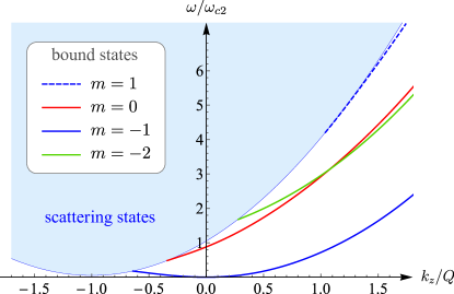
Figure 1: Linear spin-wave spectrum of the skyrmion string for a field $h=1.05$.

II Solitary wave solution for the skyrmion string

The solitary wave solutions of the effective Lagrangian in Eq. (4) of the main text is discussed in further detail. We start with the corresponding Euler-Lagrange equations of motion that read

$$-\mathrm{i}\partial_{0}\psi= \frac{1}{2}\partial_{1}^{2}\psi-\frac{1}{4}\partial_{1}\left(|\partial_{1}\psi|^{2}\partial_{1}\psi\right),$$ (11a)

$$\mathrm{i}\partial_{0}\psi^{*}= \frac{1}{2}\partial_{1}^{2}\psi^{*}-\frac{1}{4}\partial_{1}\left(|\partial_{1}\psi|^{2}\partial_{1}\psi^{*}\right).$$ (11b)

Multiplication of Eq. (11a) by $\psi^{*}$ and Eq. (11b) by $-\psi$ and subsequent summation yields the conservation law

$$\partial_{\mu}j_{\mu}=0,$$ (12)

with the density $j_{0}$ and the associated current $j_{1}$ given by

$$j_{0}= |\psi|^{2},$$ (13a)

$$j_{1}= \frac{\mathrm{i}}{2}(\psi\partial_{1}\psi^{*}-\psi^{*}\partial_{1}\psi)\left(1-\frac{1}{2}|\partial_{1}\psi|^{2}\right).$$ (13b)

For appropriate boundary conditions the total number of particles $N=\int|\psi|^{2}\mathrm{d}x_{1}$ is constant in time. Moreover, the symmetry with respect to space-time translations leads to the conservation law

$$\partial_{\mu}T_{\mu\nu}=0$$ (14)

for the energy-momentum tensor

$$T_{\mu\nu}=-\delta_{\mu\nu}\mathcal{L}+\frac{\partial\mathcal{L}}{\partial\partial_{\mu}\psi}\partial_{\nu}\psi+\frac{\partial\mathcal{L}}{\partial\partial_{\mu}\psi^{*}}\partial_{\nu}\psi^{*}.$$ (15)

Consequently, the total energy $E=\int T_{00}\mathrm{d}x_{1}$ and total linear momentum $P=-\int T_{01}\mathrm{d}x_{1}$ are constant in time. The components of the energy-momentum tensor read explicity

$$\begin{split}T_{00}&=\frac{1}{2}|\partial_{1}\psi|^{2}-\frac{1}{8}|\partial_{1}\psi|^{4},\\ T_{01}&=\frac{\mathrm{i}}{2}(\psi^{*}\partial_{1}\psi-\psi\partial_{1}\psi^{*}),\\ T_{10}&=-\frac{\mathrm{1}}{2}(\partial_{0}\psi^{*}\partial_{1}\psi+\partial_{0}\psi\partial_{1}\psi^{*})\left(1-\frac{1}{2}|\partial_{1}\psi|^{2}\right),\\ T_{11}&=-\frac{\mathrm{i}}{2}(\psi^{*}\partial_{0}\psi-\psi\partial_{0}\psi^{*})-\frac{1}{2}|\partial_{1}\psi|^{2}+\frac{3}{8}|\partial_{1}\psi|^{4}.\end{split}$$ (16)

For the Ansatz of the solitary wave function given in Eq. (5) of the main text with velocity $v$, all these components $T_{\mu\nu}$ as well as $j_{\mu}$ are reduced to functions of the variable $\xi=x_{1}-vx_{0}$. The conservation laws (12) and (14) then imply that the following quantities are independent of space and time,

$$\mathcal{J}= -vj_{0}+j_{1}=A^{2}\left[\phi^{\prime}-(\phi^{\prime}+v)\frac{|\psi^{\prime}|^{2}}{2}\right],$$ (17a)

$$\mathcal{T}_{0}= -vT_{00}+T_{10}=\frac{v}{2}|\psi^{\prime}|^{2}\left(1-\frac{3}{4}|\psi^{\prime}|^{2}\right)$$ (17b)

$$+A^{2}\left(\omega-\frac{v^{2}}{2}\right)(\phi^{\prime}+v)\left(1-\frac{|\psi^{\prime}|^{2}}{2}\right),$$

$$\mathcal{T}_{1}= -vT_{01}+T_{11}=$$ (17c)

$$-\frac{|\psi^{\prime}|^{2}}{2}\left(1-\frac{3}{4}|\psi^{\prime}|^{2}\right)-A^{2}\left(\omega-\frac{v^{2}}{2}\right),$$

where $|\psi^{\prime}|^{2}=A^{\prime 2}+A^{2}(\phi^{\prime}+v)^{2}$. These quantities are linearly dependent $\mathcal{T}_{0}+v\mathcal{T}_{1}=(\omega-\frac{v^{2}}{2})\mathcal{J}$.

In case of a spatially localized solution with boundary conditions $A(\pm\infty)=0$ and $A^{\prime}(\pm\infty)=0$ these constants vanish $\mathcal{J}=\mathcal{T}_{1}=\mathcal{T}_{2}=0$. Solving now any two equations of (17) for $A$ and $A^{\prime}$ one obtains Eqs. (6) of the main text. The resulting ordinary differential equation for the derivative of the phase $\phi^{\prime}(\xi)=v\kappa(\xi)$ reads in terms of the auxiliary localized function $\kappa(\xi)$ centered at $\xi=0$

$$\kappa^{\prime}=-\text{sgn}(\xi)|v|\frac{\kappa(1+\kappa)^{3/2}\sqrt{(2-\kappa)(2\alpha-\kappa+\kappa^{2})}}{1-2\kappa},$$ (18a)

$$\kappa(0)=(1-\sqrt{1-8\alpha})/2.$$ (18b)

where $\alpha=-2\omega/v^{2}$. The initial condition (18b) originates from the condition $A^{\prime}(0)=0$ that the derivative of the magnitude vanishes at the center of the solitary wave. Note that the initial condition is formulated for the point $\xi=0$, which is exactly at the boundary of the definitional domain of the right-hand side of Eq. (18a). The assumptions of the Peano existence theorem [9] are therefore not fulfilled, and the Cauchy differential problem (18) can have more than one solution. As a consequence, in addition to the trivial solution $\kappa(\xi)\equiv\kappa(0)=\text{const}$, one obtains the localized one with $\kappa(\pm\infty)=0$, see Fig. 2(a). Substitution of $\phi^{\prime}=v\kappa$ into Eq. (6) of the main text results in the phase trajectory shown in Fig. 2(b) and the magnitude shown in Fig. 2(c). The phase kink shown in Fig. 2(d) is obtained by computing the integral $\phi(\xi)=v\int_{0}^{\xi}\kappa(\xi^{\prime})\mathrm{d}\xi^{\prime}$.

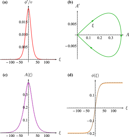
Figure 2: Solitary wave of the skyrmion string with velocity $v=0.5$ and parameter $\alpha=0.01$. (a) Solution for the derivative of the phase, $\phi^{\prime}(\xi)=v\kappa(\xi)$, obtained by solving Eq. (18). (b) The corresponding trajectory in the $(A,A^{\prime})$-plane using Eq. (6) of the main text. (c) The magnitude and (d) the phase of the solitary wave. The dashed lines in panel (c) and (d) show the low-amplitude approximations given in Eq. (8) of the main text.

In the limit $\alpha\to 0^{+}$, the total energy of the solitary wave is given by $E\approx\frac{4\sqrt{\alpha}}{|v|}$, the total momentum reads $P\approx\frac{8\sqrt{\alpha}}{v|v|}$ and the total number of particles is $N\approx 8\sqrt{\alpha}/v^{3}$. The latter quantifies the total angular momentum of the skyrmion string, $J_{z}\propto N$.

III Micromagnetic simulations

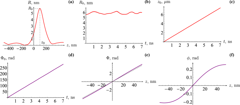
Figure 3: Numerically extracted profile of the solitary wave for the example given in Fig. 1 of the main text with positive velocity $v>0$. (a) Spatial distribution of the magnitude $R=|X+\mathrm{i}Y|$ at time $t=6.4$ ns. It shows a localized excitation with amplitude $R_{0}$ and position $z_{0}$ that both evolve in time as shown in panels (b) and (c), respectively. (d) Time evolution of the phase $\varPhi_{0}=\text{arg}(X_{0}+\mathrm{i}Y_{0})$ at the center of the solitary wave, $(X_{0},Y_{0})=(X(z_{0}),Y(z_{0}))$. (e) Spatial distribution of the phase within the comoving frame of reference $\varPhi(z)=\text{arg}[X(z-z_{0})+\mathrm{i}Y(z-z_{0})]-\varPhi_{0}$ within the region $|z-z_{0}|<\xi_{w}$, where $\xi_{w}$ is the width of the solitary wave, at time $t=6.4$ ns. The dashed line is given by $k_{z}^{\rm sw}z$ with $k_{z}^{\rm sw}=QV/V_{0}$, see text, and the difference $\phi(z)=\varPhi(z)-k_{z}^{\rm sw}z$ is shown in panel (f).

The micromagnetic simulations were performed with the OOMMF code [10] supplemented with the extension for the Dzyaloshinskii-Moriya interaction (DMI) in cubic crystals [11]. We used the parameters for the cubic chiral magnet FeGe with four Fe and four Ge atoms per unit cell that were given in Ref. 12: exchange constant $A=8.78\times 10^{-12}$ J/m, saturation magnetization $M_{s}=3.84\times 10^{5}$ A/m, and DMI constant $D=1.58\times 10^{-3}$ J/m². Magnetic field $\mu_{0}H=0.8$ T was fixed for all simulations. The magnetostatic interaction was neglected. These material parameters determine the length scale $Q^{-1}\approx 11.1$ nm and the time scale $\omega_{c2}^{-1}\approx 15.3$ ps.

We simulated the magnetization dynamics within a cylinderically shaped sample oriented along the field with a diameter 100 nm and the length was varied from 0.8 to 5 $\mu$m depending on the width of the solitary wave. For most of the cases the spatial discretization was fixed to $(\Delta x,\Delta y,\Delta z)=(1\,\text{nm},1\,\text{nm},3\,\text{nm})$. This enabled us to consider skyrmion string excitations with deformation gradients up to $|\partial_{z}\bm{R}|_{\text{max}}\approx 0.25$. For larger deformations we observed that the string broke producing a pair of oppositely charged Bloch points that quickly separated. For the largest samples the spatial discretization was increased to $(\Delta x,\Delta y,\Delta z)=(2\,\text{nm},2\,\text{nm},5\,\text{nm})$.

Periodic boundary conditions were applied to the top and bottom surfaces of the cylinder so that the skyrmion string is effectively forming a loop. At the side surfaces of the cylinder we employed Dirichlet boundary conditions with a magnetization pointing along the field, $\bm{n}=\hat{\bm{z}}$. Open boundary conditions on the side surfaces would have the disadvantage that the magnetization twists at the boundary [13] effectively reducing the lateral size of the sample.

Each simulation was performed in two steps: $(i)$ an initial magnetization $\bm{n}_{\text{ini}}(\bm{r})$ was generated containing a solitary wave of a form close to the one expected theoretically. This magnetization was relaxed using the Landau-Lifshitz-Gilbert equation with a large damping parameter $\alpha_{\textsc{g}}=0.5$ for several tens of picoseconds. $(ii)$ Afterwards the damping was switched off, $\alpha_{\textsc{g}}=0$, and the simulation was continued for a total time which varied from 7 to 40 ns depending on the velocity of the solitary wave.

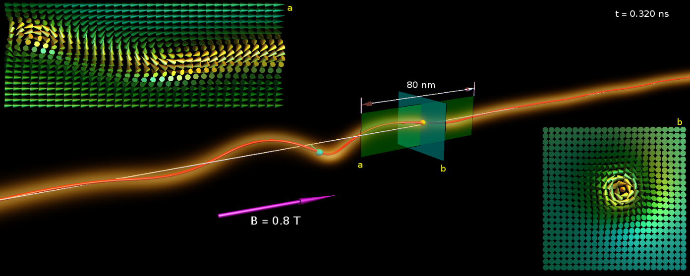
Figure 4: Snapshot of the movie movie2.mkv showing the dynamics of the solitary wave, whose parameters are marked by the superscript ^m in Table 1. The red line shows the position of the skyrmion string as defined by Eq. (2) of the main text. The color density represents the distribution of the topological charge $\rho_{\rm top}$. Panels ‘a’ and ‘b’ show the distribution of the magnetization along the cross sections determined by the planes ‘a’ and ‘b’, respectively. The cyan point has coordinates $(X_{0},Y_{0},z_{0})$ and shows the position of the solitary-wave maximum. The yellow point has coordinates $(X(0),Y(0),0)$ and shows the intersection of the string and the plane ‘b’. Note the opposite sense of rotation of the cyan and yellow points in the movie. This follows directly from the structure of the Galilean transformation of the wavefunction in Eq. (5) of the main text. Whereas the cyan point in the comoving frame of reference is expected to rotate with the dimensionless frequency $\omega-v^{2}/2=-(1+\alpha)v^{2}/2<0$ that is negative, the yellow point in the fixed frame of reference instead rotates on average with a positive frequency $\omega+v^{2}/2=(1-\alpha)v^{2}/2>0$ for $0<\alpha<1/8$. No scalings of length are applied here.

III.1 Determination of the solitary wave profile

During the second stage $(ii)$ of the simulation the magnetization snapshots were saved at timesteps $\Delta t=10$ ps. From each snapshot we extracted the skyrmion string coordinates $X$ and $Y$ by means of Eq. (2) of the main text, with which we numerically constructed the function $\Psi_{\rm sim}(z,t)=X(z,t)+\mathrm{i}Y(z,t)$. A typical profile of the solitary wave defined by the magnitude $R(z,t)=|\Psi_{\rm sim}(z,t)|$ as a function of $z$ at a certain fixed time $t$ is shown in Fig. 3(a). From the profile function $R(z,t)$ we extracted three time-dependent quantities: the amplitude $R_{0}(t)=\max_{z}R(z,t)$, the position $z_{0}(t):\,R_{0}(t)=R(z_{0}(t),t)$, and the width $\xi_{w}(t)$ by means of fitting $R(z,t)$ with the trial function $R^{\rm fit}(z)=R_{0}/\cosh(\frac{z-z_{0}}{\xi_{w}})$ at each moment of time. Results for $R_{0}(t)$ and $z_{0}(t)$ are shown in Fig. 3(b) and (c), respectively. Due to parasitic magnon excitations the amplitude $R_{0}(t)$ weakly fluctuates around a time-independent constant value $\langle R_{0}\rangle_{t}$. The time averaged amplitude $\langle R_{0}\rangle_{t}$ and width $\langle\xi_{w}\rangle_{t}$ are listed in Table 1.

Moreover, fitting the dependence $z_{0}(t)$ by a linear function $z_{0}^{\rm fit}(t)=Vt+z_{0}^{\rm ini}$, we obtain the velocity $V$, that is also listed in Table 1. In order to determine the rotation frequency $\Omega$ of the solitary wave within the comoving frame of reference, we considered the phase $\varPhi_{0}(t)=\text{arg}[X_{0}(t)+\mathrm{i}Y_{0}(t)]$ of the solitary wave at its center, where $X_{0}(t)=X(z_{0}(t),t)$ and $Y_{0}(t)=Y(z_{0}(t),t)$, see Fig. 3(d). Fitting the time dependence $\varPhi_{0}(t)$ by the linear function $\varPhi_{0}^{\rm fit}(t)=\Omega t+\varPhi_{0}^{\rm ini}$ yields the frequency $\Omega$, see Table 1. In addition, we determined the phase within the comoving frame of reference $\varPhi(z)=\text{arg}[X(z-z_{0})+\mathrm{i}Y(z-z_{0})]-\varPhi_{0}$, see Fig. 3(e). Due to parasitic magnon excitations, the phase $\varPhi(z)$ exhibits fluctuations, which are small within the region of the solitary wave $|z-z_{0}|<\xi_{w}$, but they are significant outside this region $|z-z_{0}|>\xi_{w}$ (not shown). The derivative of the phase at the center of the solitary wave averaged over time $\langle\varPhi^{\prime}(0)\rangle_{t}$ is listed in Table 1.

With this procedure we constructed the solitary wave function

$$\Psi_{\rm sim}(z,t)=R(z-Vt)e^{\mathrm{i}\varPhi(z-Vt)+\mathrm{i}\Omega t}.$$ (19)

Comparison of Eq. (19) with Eq. (5) of the main text allows to connect the numerical data with our analytical results. The magnitude function $A$ is related to $R$ via $A=RQ\sqrt{2b_{1}/a_{1}}$ with the coefficients $a_{1}$ and $b_{1}$ defined in Fig. 3 of the main text. The dimensionless velocity is given by $v=V/V_{0}$ where $V_{0}=\Omega_{0}/Q\approx 1308$ m/s, and $\Omega_{0}=2a_{1}\omega_{c2}\approx 1.177\times 10^{11}$ rad/s. With the help of the rotation frequency $\Omega$ and the velocity $V$ we can extract the dimensionless frequency $\omega=\frac{V^{2}}{2V_{0}^{2}}-\Omega/\Omega_{0}$, from which follows the dimensionless parameter $\alpha=-2\omega/v^{2}=2\frac{\Omega V_{0}^{2}}{\Omega_{0}V^{2}}-1$ that is a central quantity in the theoretical description, see Fig. (4) of the main text.

The solitary wave phase profile $\phi(z)$ is determined as $\phi(z)=\varPhi(z)-k_{z}^{\rm sw}z$, where $k_{z}^{\rm sw}=QV/V_{0}$ can be interpreted as a wavevector associated with the solitary wave.

III.2 Movies of the solitary wave

For better illustration of the solitary wave dynamics we provide three movies constructed from our micromagnetic simulations.

movie1.mkv shows the full time evolution of the snapshots given in Fig. 1 of the main text. Shown are 3 ns of the dynamics of two solitary waves moving in opposite directions. The length of the cylinder is 0.96 $\mu$m with periodic boundary conditions at the top and the bottom. Lengths in the $(x,y)$-plane are upscaled by a factor of five as in Fig. 1 of the main text. The vertical arrow indicates the direction of the magnetic field $\bm{B}=\hat{\bm{z}}$(0.8 T).

movie2.mkv illustrates the solitary wave with the largest amplitude of all simulated waves. The corresponding parameters are marked by the superscript ^m in Table 1. Shown are 0.8 ns of its dynamics; details are explained in Fig. 4.

movie3.mkv is an alternative representation of the dynamics shown in movie2.mkv. The local gyrovector field $\bm{\rho}=\hat{\bm{x}}_{i}\epsilon_{ijk}\bm{n}\cdot\left[\partial_{x_{j}}\bm{n}\times\partial_{x_{k}}\bm{n}\right]/(8\pi)$ was evaluated from the magnetization field, and it is shown by the green arrows in addition to the red line that represents Eq. (2) of the main text as in the previous two movies. The spatial distribution of the quantity $|\bm{\rho}|$ is represented both by the length of the green arrows as well as by the color density. Note that the vector $\bm{\rho}$ is tangential to the string as defined by the red line.

Velocity $V$, km/s	Frequency of rotation in the comoving r.f. $\Omega$, GHz	Amplitude $R_{0}$, nm	Half-width $\xi_{w}$, nm	Derivative of the phase at the solitary-wave center $\varPhi^{\prime}(0)$, nm-1
${}^{\rm m}0.93286\pm 6.3\times 10^{-5}$	$5.305\pm 7.4\times 10^{-4}$	$9.6\pm 0.3$	$37\pm 2$	$0.0846\pm 0.0024$
$1.00468\pm 8.1\times 10^{-5}$	$5.754\pm 8.2\times 10^{-4}$	$6.8\pm 0.3$	$53\pm 4$	$0.0776\pm 0.0011$
$1.06104\pm 1.0\times 10^{-4}$	$6.331\pm 1.2\times 10^{-3}$	$6.0\pm 0.2$	$54\pm 2$	$0.07998\pm 0.0009$
$1.08760\pm 9.5\times 10^{-5}$	$6.544\pm 1.1\times 10^{-3}$	$4.6\pm 0.15$	$66\pm 5$	$0.07910\pm 0.0006$
$1.09221\pm 7.4\times 10^{-5}$	$6.594\pm 8.0\times 10^{-4}$	$3.97\pm 0.2$	$71\pm 11$	$0.07948\pm 0.0005$
$1.10592\pm 9.5\times 10^{-5}$	$6.679\pm 1.0\times 10^{-3}$	$3.33\pm 0.13$	$82\pm 7$	$0.07870\pm 0.00032$
$1.13773\pm 3.7\times 10^{-4}$	$6.962\pm 4.4\times 10^{-3}$	$2.0\pm 0.05$	$152\pm 3$	$0.07800\pm 0.00032$
$-0.87884\pm 7.3\times 10^{-5}$	$4.8607\pm 9.2\times 10^{-4}$	$8.7\pm 0.2$	$45\pm 2$	$-0.07858\pm 0.0012$
$-0.93909\pm 7.0\times 10^{-5}$	$5.3946\pm 8.5\times 10^{-4}$	$7.0\pm 0.2$	$51\pm 2$	$-0.07915\pm 0.0009$
$-0.97287\pm 1.0\times 10^{-4}$	$5.6623\pm 1.2\times 10^{-3}$	$5.6\pm 0.2$	$62\pm 4$	$-0.07844\pm 0.0007$
$-0.99312\pm 6.6\times 10^{-5}$	$5.8445\pm 6.2\times 10^{-4}$	$4.6\pm 0.15$	$69\pm 6$	$-0.07864\pm 0.0004$
$-1.00521\pm 8.7\times 10^{-5}$	$5.9478\pm 9.8\times 10^{-4}$	$3.7\pm 0.17$	$82\pm 9$	$-0.07868\pm 0.0004$
$-1.01561\pm 9.3\times 10^{-5}$	$6.0325\pm 9.2\times 10^{-4}$	$3.17\pm 0.07$	$90\pm 4$	$-0.07831\pm 0.0002$
$-1.02910\pm 2.2\times 10^{-4}$	$6.1414\pm 2.7\times 10^{-4}$	$2.18\pm 0.05$	$137\pm 7$	$-0.07814\pm 0.0002$
$0.54606\pm 1.6\times 10^{-5}$	$1.6716\pm 7.0\times 10^{-5}$	$8.6\pm 0.4$	$122\pm 13$	$0.04051\pm 0.0003$
$0.55616\pm 1.6\times 10^{-5}$	$1.7112\pm 8.0\times 10^{-5}$	$7.4\pm 0.5$	$144\pm 23$	$0.04013\pm 0.0003$
$0.56497\pm 2.0\times 10^{-5}$	$1.7473\pm 1.0\times 10^{-4}$	$6.4\pm 0.5$	$172\pm 34$	$0.03991\pm 0.0002$
$0.57265\pm 1.6\times 10^{-5}$	$1.7792\pm 9.0\times 10^{-5}$	$5.1\pm 0.4$	$230\pm 46$	$0.03964\pm 0.0002$
$0.57995\pm 1.5\times 10^{-5}$	$1.8122\pm 9.0\times 10^{-5}$	$4.0\pm 0.3$	$272\pm 61$	$0.03952\pm 0.0001$
$-0.52443\pm 1.6\times 10^{-5}$	$1.5837\pm 7.0\times 10^{-5}$	$8.1\pm 0.3$	$137\pm 12$	$-0.04009\pm 0.0002$
$-0.53174\pm 1.4\times 10^{-5}$	$1.6127\pm 7.0\times 10^{-5}$	$7.2\pm 0.4$	$153\pm 20$	$-0.03990\pm 0.0002$
$-0.53787\pm 1.6\times 10^{-5}$	$1.6382\pm 9.0\times 10^{-5}$	$6.1\pm 0.4$	$188\pm 29$	$-0.03971\pm 0.0002$
$-0.54429\pm 1.6\times 10^{-5}$	$1.6653\pm 1.0\times 10^{-4}$	$5.0\pm 0.4$	$227\pm 39$	$-0.03956\pm 0.0001$
$-0.55005\pm 1.6\times 10^{-5}$	$1.6915\pm 9.0\times 10^{-5}$	$3.7\pm 0.4$	$308\pm 65$	$-0.03944\pm 0.0001$
$0.40583\pm 1.8\times 10^{-5}$	$0.9111\pm 8.8\times 10^{-5}$	$9.8\pm 0.7$	$211\pm 39$	$0.02916\pm 0.0002$
$0.40978\pm 2.7\times 10^{-5}$	$0.9234\pm 1.1\times 10^{-4}$	$9.1\pm 0.3$	$198\pm 14$	$0.02905\pm 0.0001$
$0.41341\pm 2.4\times 10^{-5}$	$0.9334\pm 8.8\times 10^{-5}$	$8.0\pm 0.2$	$233\pm 18$	$0.02888\pm 0.00004$
$0.41621\pm 1.7\times 10^{-5}$	$0.9402\pm 7.0\times 10^{-5}$	$6.77\pm 0.09$	$272\pm 4$	$0.02870\pm 0.00003$
$0.41898\pm 2.1\times 10^{-5}$	$0.9483\pm 8.5\times 10^{-5}$	$5.65\pm 0.09$	$330\pm 15$	$0.02857\pm 0.00003$
$-0.39226\pm 2.2\times 10^{-5}$	$0.8714\pm 1.0\times 10^{-4}$	$9.7\pm 0.5$	$210\pm 26$	$-0.02909\pm 0.00013$
$-0.39558\pm 2.2\times 10^{-5}$	$0.8810\pm 8.2\times 10^{-5}$	$8.7\pm 0.3$	$225\pm 20$	$-0.02894\pm 0.00006$
$-0.39828\pm 1.9\times 10^{-5}$	$0.8884\pm 6.8\times 10^{-5}$	$7.6\pm 0.2$	$258\pm 13$	$-0.02879\pm 0.00003$
$-0.40065\pm 1.6\times 10^{-5}$	$0.8944\pm 6.1\times 10^{-5}$	$6.38\pm 0.03$	$307\pm 5$	$-0.02864\pm 0.00003$
$-0.40238\pm 1.9\times 10^{-5}$	$0.89901\pm 8.1\times 10^{-5}$	$5.4\pm 0.2$	$354\pm 26$	$-0.02854\pm 0.00003$

Table 1: Parameters of the solitary wave extracted from micromagnetic simulations. Superscript ^m marks the solitary wave whose dynamics is illustrated in the movie movie2.mkv, see Fig. 4.

References

- Ivanov et al. [1996] B. A. Ivanov, A. K. Kolezhuk, and G. M. Wysin, Phys. Rev. Lett. 76, 511 (1996).
- Ivanov et al. [1999] B. A. Ivanov, V. M. Murav’ev, and D. D. Sheka, JETP 89, 583 (1999).
- Sheka et al. [2001] D. D. Sheka, B. A. Ivanov, and F. G. Mertens, Phys. Rev. B 64, 024432 (2001).
- Schütte and Garst [2014] C. Schütte and M. Garst, Phys. Rev. B 90, 094423 (2014).
- [5] S.-Z. Lin, J.-X. Zhu, and A. Saxena, arXiv:1901.03812 .
- Tyablikov [1975] S. V. Tyablikov, Methods in the Quantum Theory of Magnetism, 2nd ed. (Moscow, Nauka, 1975) [transl. of 1st Russ. ed., Plenum Press, New York (1967)].
- Bogdanov and Hubert [1994] A. Bogdanov and A. Hubert, J. Magn. Magn. Mater 138, 255 (1994).
- Kravchuk et al. [2018] V. P. Kravchuk, D. D. Sheka, U. K. Rößler, J. van den Brink, and Y. Gaididei, Phys. Rev. B 97, 064403 (2018).
- Peano [1890] G. Peano, Mathematische Annalen 37, 182 (1890).
- [10] “The Object Oriented MicroMagnetic Framework,” Developed by M. J. Donahue and D. Porter mainly, from NIST. We used the 3D version of the 2.00 release.
- Cortés-Ortuño et al. [2018] D. Cortés-Ortuño, M. Beg, V. Nehruji, R. A. Pepper, and H. Fangohr, “Oommf extension: Dzyaloshinskii-moriya interaction (dmi) for crystallographic classes t and o,” (2018).
- Beg et al. [2015] M. Beg, R. Carey, W. Wang, D. Cortés-Ortuño, M. Vousden, M.-A. Bisotti, M. Albert, D. Chernyshenko, O. Hovorka, R. L. Stamps, and H. Fangohr, Scientific Reports 5, 17137 (2015).
- Rohart and Thiaville [2013] S. Rohart and A. Thiaville, Phys. Rev. B 88, 184422 (2013).