Supplemental Material for: ”Spectral gaps and mid-gap states in random quantum master equations”

In this supplementary document, we provide a detailed discussion of the symmetries of the master equation and of its eigenvalue distribution in the perturbative small and large $\gamma$ limits. We also present supplemental numerical results on the eigenvalue distribution and on finite-size gaps.

I Symmetries and perturbation theory

I.1 Statement of the problem

We consider the quantum master equation for the density matrix $\rho$ in the case of a single Hermitian jump operator

$$\partial_{t}\rho=-i[H,\rho]-\gamma\left[\frac{1}{2}\{L^{2},\rho\}-L\rho L\right]=-i[H,\rho]-\frac{\gamma}{2}[L,[L,\rho]].$$ (1)

Furthermore, we assume that the Hamiltonian $H$ and the jump operator $L$ are represented by $N\times N$ real symmetric random matrices drawn from the GOE ensemble, i.e.,

$$P(H)\propto\exp\left(-\frac{N}{2}{\rm Tr}\left[H^{2}\right]\right),\quad\langle H_{ij}H_{kl}\rangle=\frac{1}{2N}(\delta_{ik}\delta_{jl}+\delta_{ik}\delta_{jl}),$$ (2)

and similarly for $L$. Note that we have scaled the variance of the probability distribution (2) by the dimension of the Hilbert space, $N$, such that in the large-$N$ limit the spectrum of $H$ and $L$ resides within the segment $[-\sqrt{2},\sqrt{2}]$.

The master equation (1) can be written in terms of a Lindbladian superoperator, $\mathcal{L}$, represented by an $N^{2}\times N^{2}$ matrix with composite indices $ij$ and $kl$, acting on $\rho$

$$\partial_{t}\rho_{ij}=\sum_{kl}\mathcal{L}_{ij{\>\!}kl}\,\rho_{kl},$$ (3)

with

$$\mathcal{L}_{ij{\>\!}kl}=-[iH+\frac{\gamma}{2}L^{2}]_{ik}\delta_{jl}+\delta_{ik}[iH-\frac{\gamma}{2}L^{2}]_{jl}+\gamma L_{ik}L_{jl}.$$ (4)

For Hermitian jump operators, the fact that the dissipator can be written as a nested commutator implies that the Lindblad superoperator has the structure

$$\mathcal{L}=-iC_{H}-\frac{\gamma}{2}C_{L}^{2}\;,$$ (5)

where $C_{M}=M\otimes\mathbbm{1}-\mathbbm{1}\otimes M$ is the superoperator representation of the commutator with $M$. When $M$ is Hermitian, $C_{M}$ is also Hermitian.

Our goal is to explore the spectral properties of $\mathcal{L}$ as function of the dissipation strength $\gamma$. In particular, we are interested in its spectral gap, as defined below, which governs the slowest decay of the system towards a steady state.

I.2 Properties and representation of $\mathcal{L}$

The Lindblad superoperator has in general the following properties which we make use of:

1. $\mathcal{L}_{ij{\>\!}kl}=\mathcal{L}^{*}_{\widebar{ij}{\>\!}\widebar{kl}}$, where $\widebar{ij}=ji$. Thus, $\mathcal{L}_{ij{\>\!}\widebar{ij}}$ is real. In the language of linear maps, this is equivalent to the condition that the Lindbladian preserves Hermiticity $\left(\mathcal{L}[\rho]\right)^{\dagger}=\mathcal{L}[\rho^{\dagger}]$.

2. The eigenvalues of $\mathcal{L}$ are either real or come in complex conjugated pairs. This follows from the item above, since if $\rho$ is an eigenmode such that $\mathcal{L}[\rho]=\lambda\rho$, then $\rho^{\dagger}$ is also an eigenmode satisfying $\mathcal{L}[\rho^{\dagger}]=\lambda^{*}\rho^{\dagger}$. In the superoperator representation, this property is a consequence of the symmetry $[\mathcal{L},{\cal C}{\cal K}]=0$, where in the block representation introduced in Eq. (8) below

   $${\cal C}=\left[\begin{array}[]{ccc}1&0&0\\ 0&0&1\\ 0&1&0\end{array}\right],$$ (6)

   and ${\cal K}$ is the complex conjugation operator. As a result, if $\rho$ is an eigenvector of $\mathcal{L}$ with eigenvalue $\lambda$, then ${\cal C}{\cal K}\rho$ is an eigenvector with eigenvalue $\lambda^{*}$.

3. The eigenvalues of $\mathcal{L}$ have a non-positive real part. While it is generally true, this property is easiest to show when $L$ is a Hermitian matrix, which is the case we consider in this paper. Let $\mathcal{L}|\rho\rangle=\lambda|\rho\rangle$, where $|\rho\rangle$ is the vectorized eigenmode of the Liouvillian. Then utilizing the representation (5), the real part of the eigenvalue satisfies

   $${\rm Re}\lambda=-\frac{\gamma}{2}\frac{\langle\rho|C_{L}^{2}|\rho\rangle}{\langle\rho|\rho\rangle}\leq 0,\quad{\rm for}\,\gamma\geq 0.$$ (7)

   The inequality follows because $C_{L}^{2}$, as the square of a Hermitian matrix, is clearly positive-semidefinite. We also see that convergence requires $\gamma\geq 0$.

4. The Lindblad equation is trace preserving, which means that ${\rm tr}\mathcal{L}[\rho]=0$. Using the tensor representation (3), this implies $\sum_{i}\mathcal{L}_{iikl}=0$ for all $k,l$.

With the additional assumption that $H$ and $L$ are real symmetric matrices, we have the following:

1. The Lindblad superoperator becomes symmetric: $\mathcal{L}_{ij{\>\!}kl}=\mathcal{L}_{kl{\>\!}ij}$.

2. The steady state $\mathcal{L}[\rho_{ss}]=0$ is the infinite temperature thermal state $\rho_{ss}=\frac{1}{N}\mathbbm{1}$. More generally, this is true when $L$ are normal matrices. Eq. (4) implies that if $[H,L]=0$ such that they share a basis of $N$ simultaneous eigenvectors $v^{\alpha}$, then $\rho_{ij}^{\alpha}=v_{i}^{\alpha}v_{j}^{\alpha}$ constitute $N$ zero modes.

3. We find it useful to order the composite indices of $\mathcal{L}$ in the following way

   $$\centering\begin{array}[]{c}\hskip 53.0pt\!\!\!\!\!\!\!\!\!\!\!\!\!\begin{array}[]{c c c}\rule{0.0pt}{21.0pt}\makebox[25.0pt][c]{$\vbox{$\,kk$\vspace{10pt}}$}&\makebox[50.0pt][c]{$\vbox{$\,kl$\vspace{10pt}}$}&\makebox[50.0pt][c]{$\vbox{$\,\widebar{kl}$\vspace{10pt}}$}\end{array}\\ \!\!\!\!\!\!\!\!\!\!\!{\cal L}=\begin{array}[]{c}\rule{0.0pt}{21.0pt}\makebox[25.0pt][c]{$\vbox{$ii$\vspace{11pt}}$}\\ \rule{0.0pt}{42.0pt}\makebox[25.0pt][c]{$\vbox{$\ij$\vspace{21pt}}$}\\ \rule{0.0pt}{42.0pt}\makebox[25.0pt][c]{$\vbox{$\widebar{ij}$\vspace{20pt}}$}\end{array}\!\!\left[\begin{array}[]{c|c|c}\rule{0.0pt}{21.0pt}\makebox[25.0pt][c]{$\vbox{$A$\vspace{10pt}}$}&\makebox[50.0pt][c]{$\vbox{$B$\vspace{10pt}}$}&\makebox[50.0pt][c]{$\vbox{$\;B^{*}$\vspace{10pt}}$}\\ \hline\cr\rule{0.0pt}{42.0pt}\makebox[25.0pt][c]{$\vbox{$B^{T}$\vspace{22pt}}$}&\makebox[50.0pt][c]{$\vbox{$C$\vspace{20pt}}$}&\makebox[50.0pt][c]{$\vbox{$D$\vspace{20pt}}$}\\ \hline\cr\rule{0.0pt}{42.0pt}\makebox[25.0pt][c]{$\vbox{$B^{\dagger}$\vspace{22pt}}$}&\makebox[50.0pt][c]{$\vbox{$\;D^{*}$\vspace{20pt}}$}&\makebox[50.0pt][c]{$\vbox{$\;C^{*}$\vspace{20pt}}$}\end{array}\right]\end{array},\vspace{5pt}\@add@centering$$ (8)

   where $i<j$ and $k<l$. As a consequence of properties 1 and 5 one finds that:
   $A$ is a real symmetric $N\times N$ matrix, containing the ”populations”,
   $B$ is a complex $N\times N(N-1)/2$ matrix, and
   $C$ is a complex symmetric $N(N-1)/2\times N(N-1)/2$ matrix, which together with the complex Hermitian $N(N-1)/2\times N(N-1)/2$ matrix $D$, contains the ”coherences”.

   In this representation the steady state is $\rho_{ss}=(\overbrace{1/N,\cdots,1/N}^{N},\overbrace{0,\cdots,0}^{N(N-1)})^{T}$.

4. If all eigenvalues of $\mathcal{L}$ are distinct, as is typically expected based on the randomness of $H$ and $L$ (and in the absence of any additional symmetries), then it is diagonalizable, i.e., $\mathcal{L}=V\Lambda V^{-1}$. Here, $V$ is a matrix whose columns are the eigenvectors of $\mathcal{L}$, and $\Lambda$ is a diagonal matrix containing the corresponding eigenvalues. Since $\mathcal{L}$ is symmetric, the eigenvectors $\rho^{\alpha}$ can be made an orthonormal basis with respect to the inner product $\sum_{ij}\rho^{\alpha}_{ij}\rho^{\beta}_{ij}=\delta^{\alpha\beta}$, and that for this choice $V^{-1}=V^{T}$. Note that $\mathcal{L}$ may still be diagonalizable even in the presence of degeneracy as demonstrated by the case $[H,L]=0$.

5. $\mathcal{L}$ is guaranteed to have at least $N$ real eigenvalues. This fact is a consequence of a theorem by CarlsonCarlson65 , stating that a necessary and sufficient condition for a complex matrix $M$ to have at least $m$ real eigenvalues is the existence of a Hermitian matrix ${\cal C}$ with $|\sigma({\cal C})|=m$, such that $M{\cal C}$ is also Hermitian. Here, $\sigma$ denotes the signature. In our case, ${\cal C}$ is given by Eq. (6) and $\sigma({\cal C})=N$.

I.3 The small $\gamma$ limit

In the limit of weak dissipation the dynamics is largely governed by the Hamiltonian, while $L$ acts as a small perturbation. For this reason we choose to analyze $\mathcal{L}$ in the eigenbasis of $H$, where $H_{ij}=\epsilon_{i}\delta_{ij}$ and the components of $\mathcal{L}$ take the form

$$A_{ii{\>\!}jj}=-\gamma\left[{L^{2}}_{ij}\delta_{ij}-(L_{ij})^{2}\right],$$ (9)

$$B_{ii{\>\!}kl}=-\frac{\gamma}{2}\left[{L^{2}}_{ik}\delta_{il}+\delta_{ik}{L^{2}}_{il}-2L_{ik}L_{il}\right],$$ (10)

$$C_{ij{\>\!}kl}=i(\epsilon_{j}-\epsilon_{i})\delta_{ik}\delta_{jl}-\frac{\gamma}{2}\left[{L^{2}}_{ik}\delta_{jl}+\delta_{ik}{L^{2}}_{jl}-2L_{ik}L_{jl}\right],$$ (11)

$$D_{ij{\>\!}\widebar{kl}}=-\frac{\gamma}{2}\left[{L^{2}}_{il}\delta_{jk}+\delta_{il}{L^{2}}_{jk}-2L_{il}L_{jk}\right].$$ (12)

We will first analyze the spectrum of $A$ and of the matrix $F=\left[\begin{array}[]{cc}C&D\\ D^{*}&C^{*}\end{array}\right]$ separately, and then will consider the effects of their coupling through $B$.

I.3.1 The spectrum of $A$

Within the GOE ensemble, Eq. (2), the elements of $H$ and $L$ are normally-distributed independent random variables with zero mean $\mu(L_{ij})=0$, and standard deviation $\sigma(L_{ij})=1/\sqrt{(2-\delta_{ij})N}$. The central limit theorem then implies that in the large-$N$ limit the diagonal elements of $A_{ii}=-\gamma\sum_{j\neq i}(L_{ij})^{2}$ are normally distributed, with slight dependence between them ($L_{ij}$ appears both in $A_{ii}$ and $A_{jj}$) and

$$\mu(A_{ii})=-\gamma\frac{N-1}{2N}\simeq-\frac{\gamma}{2},\;\;\;\;\;\;\;\;\sigma(A_{ii})=\gamma\sqrt{\frac{N-1}{2N^{2}}}\simeq\frac{\gamma}{\sqrt{2N}}.$$ (13)

The off-diagonal elements are chi-squared distributed with

$$\mu(A_{ij})=\frac{\gamma}{2N},\;\;\;\;\;\;\;\;\sigma(A_{ij})=\frac{\gamma}{\sqrt{2}N},$$ (14)

and are dependent on the diagonal elements $A_{ii}$.

Next, we decompose $A$ according to

$$A=W+\frac{\gamma}{2N}K-\frac{\gamma}{2}I,$$ (15)

where $K$ is the constant matrix $K_{ij}=1$. The elements of $W$ are distributed in the same way as the elements of $A$, except that their mean is shifted to zero $\mu(W_{ij})=0$. Because $\sum_{i}W_{ij}=\sum_{j}W_{ij}=0$ one finds $[W,K]=0$, and the eigenvectors of $A$ are simultaneous eigenvectors of $W$ and $K$ (and trivially of $I$). Among them the zero mode $v^{0}=(1/N,\cdots,1/N)$ is always present and the remaining eigenvectors $v^{\alpha}$, $\alpha=1,\cdots,N-1$, are orthogonal to it and thus satisfy $\sum_{i}v^{\alpha}_{i}=0$. Consequently, $Kv^{\alpha}=0$ and their eigenvalues are $-\gamma/2+w^{\alpha}$, where $w^{\alpha}$ are the eigenvalues with respect to $W$. Since the elements of $W$, as those of $A$, are not independent the eigenvalue distribution deviates from Wigner’s semicircle law. Nevertheless, we can estimate its width. To this end, consider the eigenvalue problem $\sum_{j}W_{ij}v^{\alpha}_{j}=w^{\alpha}v^{\alpha}_{i}$, which implies $\mu(w^{\alpha})=0$, provided any correlations between $v^{\alpha}_{i}$ and $W_{ij}$ are neglected. Squaring the eigenvalue equation, summing over $i$ and using the normalization of wavevectors leads to

$$(w^{\alpha})^{2}=\sum_{ij}W_{ij}^{2}(v^{\alpha}_{j})^{2}+\sum_{i}\sum_{j\neq k}W_{ij}W_{ik}v^{\alpha}_{j}v^{\alpha}_{k}.$$ (16)

Neglecting the dependence of $v^{\alpha}_{i}$ on $W_{ij}$ one obtains

$$\mu\left[(w^{\alpha})^{2}\right]=\left[\mu\left(W_{jj}^{2}\right)+\sum_{i\neq j}\mu\left(W_{ij}^{2}\right)\right]\sum_{j}\left(v_{j}^{\alpha}\right)^{2}=\frac{\gamma^{2}}{2N}+(N-1)\frac{\gamma^{2}}{2N^{2}}\simeq\frac{\gamma^{2}}{N}.$$ (17)

Hence, we conclude that the spectrum of $A$ is narrowly distributed around $-\gamma/2$ with a width that scales as $\gamma/\sqrt{N}$. This conclusion is supported by our numerics.

The matrix $A$ is also known as a Markov generator, and was studied in some detail in Refs. Timm, ; Bryc, . In particular, it was proven in Ref. Bryc, using the method of moments that the limiting eigenvalue distribution as $N\to\infty$ is given by the sum of two delta functions: one at the origin with unit weight corresponding to the steady state, and one at $-\gamma/2$ with weight $N-1$.

I.3.2 The spectrum of $F$

Since $\gamma$ is small our strategy is to estimate the eigenvalue distribution of $F$ by treating its off-diagonal elements as a perturbation. The diagonal elements are

$$-\frac{\gamma}{2}\left[{L^{2}}_{ii}+{L^{2}}_{jj}-2L_{ii}L_{jj}\right]+i(\epsilon_{j}-\epsilon_{i})\equiv x_{ij}+iy_{ij},\;\;\;\;\;\;\;\;\;\;\;\;\;\;\;(i\neq j).$$ (18)

Using the fact that in the large-$N$ limit ${L^{2}}_{ii}$ are normally distributed with $\mu({L^{2}}_{ii})=1/2$ and $\sigma({L^{2}}_{ii})=1/\sqrt{2N}$ and neglecting the $O(1/N)$ contribution from the $L_{ii}L_{jj}$ piece, we find that the $x_{ij}$s are normally distributed with

$$\mu(x)=-\frac{\gamma}{2},\;\;\;\;\;\;\;\;\sigma(x)=\frac{\gamma}{2\sqrt{N}}.$$ (19)

On scales larger than the mean level spacing $\delta\sim 1/N$ one can largely neglect the correlations between the $\epsilon_{i}$s and evaluate the distribution of $y_{ij}$ using Wigner’s semicircle law

$$P(y_{ij})=\frac{1}{\pi^{2}}\int_{-\sqrt{2}}^{\sqrt{2}}d\epsilon\sqrt{2-\epsilon^{2}}\sqrt{2-(y_{ij}-\epsilon)^{2}}\,\Theta\left(2\sqrt{2}-|y_{ij}|\right)=f(y_{ij})\,\Theta\left(2\sqrt{2}-|y_{ij}|\right),$$ (20)

with

$$f(y)=\frac{2\sqrt{2}+|y|}{6\pi^{2}}\left\{(8+y^{2}){\cal E}\left[\left(\frac{2\sqrt{2}-|y|}{2\sqrt{2}+|y|}\right)^{2}\right]-2^{5/2}|y|{\cal K}\left[\left(\frac{2\sqrt{2}-|y|}{2\sqrt{2}+|y|}\right)^{2}\right]\right\},$$ (21)

where ${\cal E}$ and ${\cal K}$ are the complete elliptic integrals and $\Theta$ is the step function. The above result fails for $|y_{ij}|\lesssim\delta$ due to level repulsion, and in this regime $P(|y_{ij}|\lesssim\delta)\sim|y_{ij}|$. However, for the rough estimates that will follow we only need to note that Eq. (20) implies that in the large-$N$ limit

$$\mu(y)=0,\;\;\;\;\;\;\;\;\sigma(y)=1.$$ (22)

Let us consider the shift of an unperturbed eigenvalue $x_{ij}+iy_{ij}$ within second order perturbation theory. The corresponding eigenstate $\rho_{ij}$ is connected by $(N-1)^{2}-N+2$ off-diagonal elements of $F$ to other states $\rho_{kl}$ with both $k\neq i$ and $l\neq j$ (type $A$), and by $2(N-2)$ off-diagonal elements to states $\rho_{kl}$ with either $k=i$ or $l=j$ (type $B$). We begin by examining the type $A$ elements, which are of the form $z_{ij{\>\!}kl}=\gamma L_{ik}L_{jl}$, with the distribution function

$$P(z)=\frac{N}{\pi}\int_{-\infty}^{\infty}dl\frac{1}{\gamma|x|}e^{-Nl^{2}}e^{-Nz^{2}/\gamma^{2}l^{2}}=\frac{2N}{\pi\gamma}K_{0}\left(\frac{2N}{\gamma}|z|\right),$$ (23)

where $K_{0}$ is the modified Bessel function. Consequently, the numerator of the corresponding term in the eigenvalue shift

$$\frac{z_{ij{\>\!}kl}^{2}}{x_{ij}-x_{kl}+i(y_{ij}-y_{kl})}\equiv\frac{\zeta_{ij{\>\!}kl}}{x_{ij{\>\!}kl}+iy_{ij{\>\!}kl}},$$ (24)

is distributed according to

$$P^{A}_{\zeta}(\zeta)=\frac{2N}{\pi\gamma}\frac{1}{\sqrt{\zeta}}K_{0}\left(\frac{2N}{\gamma}\sqrt{\zeta}\right)\Theta(\zeta).$$ (25)

We are particularly interested in the shift of the real part of the eigenvalue due to these terms

$$\Delta x^{A}_{ij}=\sum_{k\neq i,l\neq j}\frac{x_{ij{\>\!}kl}}{x_{ij{\>\!}kl}^{2}+y_{ij{\>\!}kl}^{2}}\zeta_{ij{\>\!}kl}\equiv\sum_{k\neq i,l\neq j}\xi_{ij{\>\!}kl}\zeta_{ij{\>\!}kl}\equiv\sum_{k\neq i,l\neq j}\chi_{ij{\>\!}kl},$$ (26)

as the unperturbed real part is very narrowly distributed in the large-$N$ limit, see Eq. (19). To this end we note that $x_{ij{\>\!}kl}=x_{ij}-x_{kl}$ is normally distributed with $\mu(x)=0$ and $\sigma(x)=\gamma/\sqrt{2N}$. To simplify the analysis we neglect the weak correlations between $y_{ij}$ and $y_{kl}$ and approximate the distribution of $y_{ij{\>\!}kl}=y_{ij}-y_{kl}$ by a normal distribution with $\mu(y)=0$ and $\sigma(y)=\sqrt{2}$, in accordance with Eq. (22). We have checked numerically that this is a fair approximation. Under these assumptions

$$P^{A}_{\xi}(\xi) = \frac{N^{1/2}}{2\pi\gamma}\int_{-\infty}^{\infty}dxdy\,e^{-Nx^{2}/\gamma^{2}}e^{-y^{2}/4}\delta\left(\xi-\frac{x}{x^{2}+y^{2}}\right)$$ (27)

$$= \frac{N^{1/2}}{2\pi\gamma}\frac{1}{|\xi|^{3}}\int_{-\infty}^{\infty}dy\frac{1}{(1+y^{2})^{2}}e^{-N/[\gamma^{2}\xi^{2}(1+y^{2})^{2}]}e^{-y^{2}/[4\xi^{2}(1+y^{2})^{2}]}.$$

By considering the behavior of the integrand in different regimes it is possible to approximate

$$P^{A}_{\xi}(\xi)\sim\left\{\begin{array}[]{cc}\frac{N^{1/2}}{\gamma}|\xi|^{-3}&\;\;\;\;\;\;|\xi|>\frac{N^{1/2}}{\gamma}\\ \frac{\gamma^{1/2}}{N^{1/4}}|\xi|^{-3/2}&\;\;\;\;\;\;\frac{N^{1/2}}{\gamma}>|\xi|>\frac{\gamma}{N^{1/2}}\\ \frac{N^{1/2}}{\gamma}&\;\;\;\;\;\;\frac{\gamma}{N^{1/2}}>|\xi|\end{array}\right..$$ (28)

Combining Eqs. (25,28) allows us to estimate the distribution of $\chi_{ij{\>\!}kl}=\xi_{ij{\>\!}kl}\zeta_{ij{\>\!}kl}$

$$P^{A}_{\chi}(\chi)=\int_{0}^{\infty}d\zeta\,\frac{1}{\zeta}P^{A}_{\zeta}(\zeta)P^{A}_{\xi}\left(\frac{\chi}{\zeta}\right)\sim\left\{\begin{array}[]{cc}\frac{\gamma^{3}}{N^{7/2}}|\chi|^{-3}&\;\;\;\;\;\;|\chi|>\frac{\gamma}{N^{3/2}}\\ \frac{\gamma^{3/2}}{N^{5/4}}|\chi|^{-3/2}&\;\;\;\;\;\;\frac{\gamma}{N^{3/2}}>|\chi|>\frac{\gamma^{3}}{N^{5/2}}\\ \frac{N^{5/2}}{\gamma^{3}}+\frac{N^{5/4}}{\gamma^{3/2}}|\chi|^{-1/2}\ln\left(\frac{\gamma^{3}}{N^{5/2}|\chi|}\right)&\ \;\;\;\;\;\;\frac{\gamma^{3}}{N^{5/2}}>|\chi|\end{array}\right.,$$ (29)

which implies $\mu(|\chi^{A}|)\equiv\mu(|\chi_{ij{\>\!}kl}|)\sim\gamma^{2}/N^{2}$.

Consider now the type $B$ terms with $i=k$ or $j=l$. The latter, for example, are dominated by $z_{ij{\>\!}kj}=-(\gamma/2){L^{2}}_{ik}$, which is normally distributed with $\mu(z)=0$ and $\sigma(z)=\gamma/(4\sqrt{N})$. Consequently, the numerators of the corresponding perturbative correction

$$\Delta x^{B}_{ij}=\sum_{k\neq i}\frac{x_{ij{\>\!}kj}}{x_{ij{\>\!}kj}^{2}+y_{ij{\>\!}kj}^{2}}\zeta_{ij{\>\!}kj}+\sum_{l\neq j}\frac{x_{ij{\>\!}il}}{x_{ij{\>\!}il}^{2}+y_{ij{\>\!}il}^{2}}\zeta_{ij{\>\!}il}\equiv\sum_{k\neq i}\xi_{ij{\>\!}kj}\zeta_{ij{\>\!}kj}+\sum_{l\neq j}\xi_{ij{\>\!}il}\zeta_{ij{\>\!}il}\equiv\sum_{k\neq i}\chi_{ij{\>\!}kj}+\sum_{l\neq j}\chi_{ij{\>\!}il},$$ (30)

are distributed according to

$$P^{B}_{\zeta}(\zeta)=\frac{4\sqrt{N}}{\sqrt{2\pi}\gamma}\frac{1}{\sqrt{\zeta}}e^{-(8N/\gamma^{2})\zeta}\,\Theta(\zeta).$$ (31)

The real part of the denominator $x_{ij{\>\!}kj}\approx-(\gamma/2)({L^{2}}_{ii}-{L^{2}}_{kk})$ is normally distributed with $\mu(x)=0$ and $\sigma(x)=\gamma/(2\sqrt{N})$. We approximate the distribution of the imaginary part $y_{ij{\>\!}kj}=\epsilon_{k}-\epsilon_{i}$, Eq. (20), by a normal distribution with $\mu(y)=0$ and $\sigma(y)=1$. Consequently, the distribution $P^{B}_{\xi}(\xi)$ of $\xi_{ij{\>\!}kj}$ and $\xi_{ij{\>\!}il}$ shares the same approximate begavior of $P^{A}_{\xi}(\xi)$, as given by Eq. (28), and for $\chi_{ij{\>\!}kj}$, $\chi_{ij{\>\!}jl}$ we may estimate

$$P^{B}_{\chi}(\chi)=\int_{0}^{\infty}d\zeta\,\frac{1}{\zeta}P^{B}_{\zeta}(\zeta)P^{B}_{\xi}\left(\frac{\chi}{\zeta}\right)\sim\left\{\begin{array}[]{cc}\frac{\gamma^{3}}{N^{3/2}}|\chi|^{-3}&\;\;\;\;\;\;|\chi|>\frac{\gamma}{N^{1/2}}\\ \frac{\gamma^{3/2}}{N^{3/4}}|\chi|^{-3/2}&\;\;\;\;\;\;\frac{\gamma}{N^{1/2}}>|\chi|>\frac{\gamma^{3}}{N^{3/2}}\\ \frac{N^{3/4}}{\gamma^{3/2}}|\chi|^{-1/2}&\;\;\;\;\;\;\frac{\gamma^{3}}{N^{3/2}}>|\chi|\end{array}\right.,$$ (32)

implying $\mu(|\chi^{B}|)\equiv\mu(|\chi_{ij{\>\!}kj}|)=\mu(|\chi_{ij{\>\!}il}|)\sim\gamma^{2}/N$.

Finally, ignoring the dependence of $|\chi_{ij{\>\!}kl}|$ on the position of the unperturbed levels within the spectrum we may approximate

$$\mu(\Delta x_{ij}) = \mu(\Delta^{A}x_{ij})+\mu(\Delta^{B}x_{ij})$$ (33)

$$\sim \mu(|\chi^{A}|)\sum_{k\neq i,l\neq j}{\rm sign}(\chi_{ij{\>\!}kl})+\mu(|\chi^{B}|)\Bigg{[}\sum_{k\neq i}{\rm sign}(\chi_{ij{\>\!}kj})+\sum_{l\neq j}{\rm sign}(\chi_{ij{\>\!}il})\Bigg{]}\sim\gamma^{2}{\rm erf}\left(\frac{x_{ij}+\gamma/2}{\gamma/\sqrt{2N}}\right).$$

Here we used the fact that owing to the normal distribution of the $x_{ij}$s, a state with a given $x_{ij}$ has a proportion of $1/2\pm(1/2){\rm erf}[(x_{ij}+\gamma/2)/({\gamma/\sqrt{2N}})]$ of the terms in the sum appear with sign $\pm 1$.

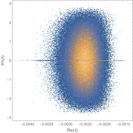
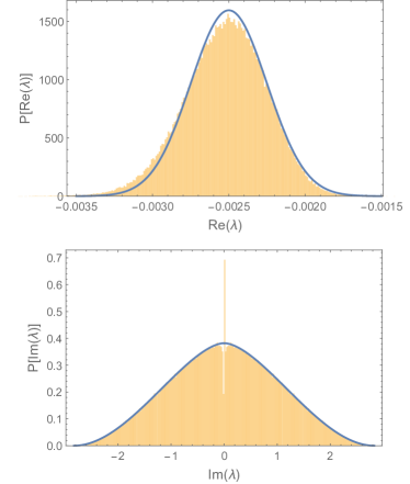
Figure 1: Left: Eigenvalue distribution of $\mathcal{L}$, binned from 40 realizations for the case $\gamma=0.005$ and $N=100$. Not shown is the zero-mode at the origin. Right: Projections of the distribution on the real and imaginary axes. The former is concentrated around $-\gamma/2$ and for the range of parameters used its standard deviation is $\gamma/(2\sqrt{N})$. The blue line depicts a normal distribution with these parameters. We expect that as $N\rightarrow\infty$ the standard deviation transitions to $O(\gamma^{2})$. The imaginary parts are distributed with standard deviation 1, and the blue line depict the distribution given by Eq. (20). Note the peak due to the real eigenvalues inside the dip around zero that is inherited from the level repulsion of $H$.

As a rough estimate for the distribution of the real part of the eigenvalues $\tilde{x}_{ij}=x_{ij}+\Delta x_{ij}$ we replace $\Delta x_{ij}$ by its mean, Eq. (33), and approximate ${\rm erf}(x)\sim x$ to obtain $\tilde{x}_{ij}=x_{ij}+c\gamma\sqrt{N}(x_{ij}+\gamma/2)$, where $c$ is a constant of order 1. The resulting $\tilde{x}_{ij}$ is normally distributed with $\mu(\tilde{x})=-\gamma/2$ and a standard deviation that evolves from $\gamma/(2\sqrt{N})$ for $N\ll 1/\gamma^{2}$ to $\sigma(\tilde{x})=c\gamma^{2}/2$ for $N\gg 1/\gamma^{2}$, see Fig. 1. We note that Eqs. (29) and (32) imply that $\sigma(|\chi^{A,B}|)$ diverges logarithmically due to the behavior of $P_{\chi}$ at large values. This would lead to positive values of $\tilde{x}_{ij}$ in contradiction to their non-positiveness (see property 3 of section I.2), indicating the failure of second order perturbation theory for the edges of the distribution. The same remark also holds for the normal distribution estimated above.

Consider now the shift in the imaginary part of the eigenvalue due to the $A$-type terms

$$\Delta y^{A}_{ij}=-\sum_{k\neq i,l\neq j}\frac{y_{ij{\>\!}kl}}{x_{ij{\>\!}kl}^{2}+y_{ij{\>\!}kl}^{2}}\zeta_{ij{\>\!}kl}\equiv\sum_{k\neq i,l\neq j}\eta_{ij{\>\!}kl}\zeta_{ij{\>\!}kl}\equiv\sum_{k\neq i,l\neq j}\nu_{ij{\>\!}kl},$$ (34)

Under the same assumptions used before

$$P^{A}_{\eta}(\eta) = \frac{N^{1/2}}{2\pi\gamma}\int_{-\infty}^{\infty}dxdy\,e^{-Nx^{2}/\gamma^{2}}e^{-y^{2}/4}\delta\left(\eta+\frac{y}{x^{2}+y^{2}}\right)$$ (35)

$$= \frac{N^{1/2}}{2\pi\gamma}\frac{1}{|\eta|^{3}}\int_{-\infty}^{\infty}dx\frac{1}{(1+x^{2})^{2}}e^{-Nx^{2}/[\gamma^{2}\eta^{2}(1+x^{2})^{2}]}e^{-1/[4\eta^{2}(1+x^{2})^{2}]}.$$

By considering the behavior of the integrand in different regimes it is possible to approximate

$$P^{A}_{\eta}(\eta)\sim\left\{\begin{array}[]{cc}\frac{N^{1/2}}{\gamma}|\eta|^{-3}&\;\;\;\;\;\;|\eta|>\frac{N^{1/2}}{\gamma}\\ |\eta|^{-2}&\;\;\;\;\;\;\frac{N^{1/2}}{\gamma}>|\eta|>1\\ \frac{\gamma^{2}}{N}&\;\;\;\;\;\;1>|\eta|\end{array}\right..$$ (36)

Combining Eqs. (25,36) we can estimate

$$P^{A}_{\nu}(\nu)=\int_{0}^{\infty}d\zeta\,\frac{1}{\zeta}P^{A}_{\zeta}(\zeta)P^{A}_{\eta}\left(\frac{\nu}{\zeta}\right)\sim\left\{\begin{array}[]{cc}\frac{\gamma^{3}}{N^{7/2}}|\nu|^{-3}&\;\;\;\;\;\;|\nu|>\frac{\gamma}{N^{3/2}}\\ \frac{\gamma^{2}}{N^{2}}|\nu|^{-2}&\;\;\;\;\;\;\frac{\gamma}{N^{3/2}}>|\nu|>\frac{\gamma^{2}}{N^{2}}\\ \frac{N}{\gamma}|\nu|^{-1/2}\left[1+\ln\left(\frac{\gamma^{2}}{N^{2}|\nu|}\right)\right]&\ \;\;\;\;\;\;\frac{\gamma^{2}}{N^{2}}>|\nu|\end{array}\right..$$ (37)

Numerically, its seems that the decay in the intermediate region $\gamma/N^{3/2}>|\nu|>\gamma^{2}/N^{2}$ is slightly slower than $1/\nu^{2}$. This would eliminate the logarithmic correction to $\mu(|\nu^{A}|)\equiv\mu(|\nu_{ij{\>\!}kl}|)$ and lead to $\mu(|\nu^{A}|)\sim\gamma^{2}/N^{2}$.

The shift due to the $B$ type terms is

$$\Delta y^{B}_{ij}=-\sum_{k\neq i}\frac{y_{ij{\>\!}kj}}{x_{ij{\>\!}kj}^{2}+y_{ij{\>\!}kj}^{2}}\zeta_{ij{\>\!}kj}-\sum_{l\neq j}\frac{y_{ij{\>\!}il}}{x_{ij{\>\!}il}^{2}+y_{ij{\>\!}il}^{2}}\zeta_{ij{\>\!}il}\equiv\sum_{k\neq i}\eta_{ij{\>\!}kj}\zeta_{ij{\>\!}kj}+\sum_{l\neq j}\eta_{ij{\>\!}il}\zeta_{ij{\>\!}il}\equiv\sum_{k\neq i}\nu_{ij{\>\!}kj}+\sum_{l\neq j}\nu_{ij{\>\!}il}.$$ (38)

Due to similar reasons to the ones outlined above, the distribution $P^{B}_{\eta}(\eta)$ of $\eta_{ij{\>\!}kj}$ and $\eta_{ij{\>\!}il}$ shares the same approximate begavior of $P^{A}_{\eta}(\eta)$, as given by Eq. (36), and for $\nu_{ij{\>\!}kj}$, $\nu_{ij{\>\!}jl}$ we may estimate

$$P^{B}_{\nu}(\nu)=\int_{0}^{\infty}d\zeta\,\frac{1}{\zeta}P^{B}_{\zeta}(\zeta)P^{B}_{\eta}\left(\frac{\nu}{\zeta}\right)\sim\left\{\begin{array}[]{cc}\frac{\gamma^{3}}{N^{3/2}}|\nu|^{-3}&\;\;\;\;\;\;|\nu|>\frac{\gamma}{N^{1/2}}\\ \frac{\gamma^{2}}{N}|\nu|^{-2}&\;\;\;\;\;\;\frac{\gamma}{N^{1/2}}>|\nu|>\frac{\gamma^{2}}{N}\\ \frac{N^{1/2}}{\gamma}|\nu|^{-1/2}&\;\;\;\;\;\;\frac{\gamma^{2}}{N}>|\nu|\end{array}\right.,$$ (39)

implying (assuming that the decay in the intermediate region is slightly slower than $\nu^{-2}$, as appears numerically) that $\mu(|\nu^{B}|)\equiv\mu(|\nu_{ij{\>\!}kj}|)=\mu(|\nu_{ij{\>\!}il}|)\sim\gamma^{2}/N$.

Using these results we may approximate the shift in the imaginary part of the eigenvalues

$$\mu(\Delta y_{ij})=\mu(\Delta^{A}y_{ij})+\mu(\Delta^{y}y_{ij})\sim\mu(|\nu^{A}|)\sum_{k\neq i,l\neq j}{\rm sign}(\nu_{ij{\>\!}kl})+\mu(|\nu^{B}|)\Bigg{[}\sum_{k\neq i}{\rm sign}(\nu_{ij{\>\!}kj})+\sum_{l\neq j}{\rm sign}(\nu_{ij{\>\!}il})\Bigg{]}.$$ (40)

Away from the origin the resulting $O(\gamma^{2})$ shift is negligible compared to the $O(1)$ width of $P(y_{ij})$. There is, however, the question of the effect on the behaviour for $|y_{ij}|<1/N$, where the level repulsion of $H$ implies $P(y_{ij})\sim N|y_{ij}|$. Owing to this behavior, a given state with $|y_{ij}|<1/N$ has a proportion of $1/2\pm(N/2)y_{ij}^{2}$ of the terms in the sum appear with sign $\mp y_{ij}/|y_{ij}|$. As a result, the shift is of order $-N\gamma^{2}y_{ij}^{2}{\rm sign}(y_{ij})$, which can be neglected compared to $y_{ij}$, and level repulsion persists.

I.3.3 The effect of the $B$ couplings

The analysis of the preceding section can be readily applied to the coupling between the $A$ and $F$ sectors via the $B$ matrix. While the zero mode of $A$ is unaffected, the remaining $N-1$ eigenvalues of $A$ are shifted along the real axis. Their resulting distribution is approximately normal with $\mu(x)=-\gamma/2$ and $\sigma(x)$ that varies from $\gamma/\sqrt{N}$ to $O(\gamma^{2})$ as $N$ is increased beyond $1/\gamma^{2}$. Note that they stay real, since the perturbative corrections come in complex conjugate pairs. At the same time, the coupling through $B$ has negligible effect on the $F$ spectrum. This is a result of the fact that there are only $N-2$ type-$A$ perturbative corrections for a given $kl$, and only two type-$B$ corrections (in the original $A$ basis). This leads to a total correction that scales as $1/N$.

I.3.4 Laplace Transform and long time limit

An alternative method to track the gap structure of the eigenvalues within perturbation theory utilizes the Laplace transform of the resolvent of the Lindblad superoperator, which we define directly

$$F(t)=\left\langle{\rm tr}\,e^{\mathcal{L}t}\right\rangle=\left\langle\sum_{a}e^{\lambda_{a}t}\right\rangle.$$ (41)

Evaluating the eigenvalues to first order in perturbation theory, we can split the sum into two pieces. One controlled by the eigenvalues of $A$, and the others given by the first-order shift of the complex eigenvalues Eq. (18)

$$F(t)=\left\langle{\rm tr}e^{At}\right\rangle+\left\langle\sum_{i\neq j}e^{(x_{ij}+iy_{ij})t}\right\rangle.$$ (42)

Using the results of Ref. Bryc, , the first term tends to

$$\left\langle{\rm tr}e^{At}\right\rangle\to 1+(N-1)e^{-\frac{\gamma}{2}t}.$$ (43)

The second term can be evaluated exactly to yield

$$\left\langle\sum_{i\neq j}e^{(x_{ij}+iy_{ij})t}\right\rangle=(N^{2}-N)\left(K(t)-N\right)\left(1+\frac{2\gamma t}{N}\right)^{-1/2}\left(1+\frac{\gamma t}{N}\right)^{-1/2}\left(1+\frac{\gamma t}{2N}\right)^{-(N-2)},$$ (44)

where $K(t)$ is the spectral form factor of the Hamiltonian $H$. In the limit $N\to\infty$, this becomes exponentially decaying $\exp(-\gamma t/2)$, with a life-time identical to that produced by $A$.

I.4 The large $\gamma$ limit

In the limit of strong dissipation the dynamics is largely governed by the jump operator and we use its eigenbasis, where $L_{ij}=\kappa_{i}\delta_{ij}$, to express the components of $\mathcal{L}$ as

$$A_{ii{\>\!}jj}=0,$$ (45)

$$B_{ii{\>\!}kl}=i\left[\delta_{ik}H_{il}-H_{ik}\delta_{il}\right],$$ (48)

$$C_{ij{\>\!}kl}=-\frac{\gamma}{2}(\kappa_{i}-\kappa_{j})^{2}\delta_{ik}\delta_{jl}+i\left[\delta_{ik}H_{jl}-H_{ik}\delta_{jl}\right],$$

$$D_{ij{\>\!}\widebar{kl}}=i\left[\delta_{il}H_{jk}-H_{il}\delta_{jk}\right].$$

Here, we would like to bring $\mathcal{L}$ into a block diagonal form

$$\mathcal{L}=\left[\begin{array}[]{cc}A^{\prime}&0\\ 0&F^{\prime}\end{array}\right],$$ (49)

where $A^{\prime}$ in an $N\times N$ Hermitian matrix whose eigenvalues are the $N$ guaranteed real eigenvalues of $\mathcal{L}$, and $F^{\prime}$ is a complex symmetric $N(N-1)\times N(N-1)$ matrix. To achieve this we employ a generalized Schrieffer-Wolff transformation Kessler , which to lowest order on $1/\gamma$ gives

$$A^{\prime} = -BC_{0}^{-1}B^{T}+{\rm c.c.},$$ (50)

$$F^{\prime} = \left[\begin{array}[]{cc}C&D\\ D^{*}&C^{*}\end{array}\right],$$ (53)

where $[C_{0}]_{ij{\>\!}kl}=-(\gamma/2)(\kappa_{i}-\kappa_{j})^{2}\delta_{ik}\delta_{jl}$.

I.4.1 The spectrum of $A^{\prime}$

We are interested in finding the eigenvalues $\Lambda$ and eigenvectors ${\bm{v}}$ of $A^{\prime}$. Using Eq. (50) the eigenvalue equation becomes

$$\frac{4}{\gamma}\sum_{\begin{subarray}{c}j=1\\ j\neq i\end{subarray}}^{N}(H_{ij})^{2}\frac{v_{j}-v_{i}}{(\kappa_{j}-\kappa_{i})^{2}}=\lambda v_{i}.$$ (54)

In the $N\rightarrow\infty$ the $\kappa$s become dense, with density

$$\nu(\kappa)=\frac{N}{\pi}\sqrt{2-\kappa^{2}}\,\Theta(2-\kappa^{2}),$$ (55)

and it is useful to parameterize the eigenvector components not by the index of the corresponding basis state but by its eigenvalue $\kappa$. Furthermore, consider a window $1/N\ll\Delta\kappa\ll 1$ containing $m=\nu(\kappa)\Delta\kappa\gg 1$ levels. If $v_{j}$ do not change appreciably within this window we may approximate its contribution to the left hand side of Eq. (50) by $4(v_{j}-v_{i})/[\gamma(\kappa_{j}-\kappa_{i})^{2}]\sum_{j\in\Delta\kappa}(H_{ij})^{2}$. Since for $i\neq j$, $\mu[(H_{ij})^{2}]=1/(2N)$ and $\sigma[(H_{ij})^{2}]=1/(\sqrt{2}N)$ the central limit theorem implies that $\sum_{j\in\Delta\kappa}(H_{ij})^{2}$ is normally distributed with mean $m/(2N)$ and standard deviation $\sqrt{m}/(\sqrt{2}N)$. Consequently, we may neglect its fluctuations, replace it by its mean and arrive at the following eigenvalue problem

$$\frac{2}{\gamma N}P\int_{-\sqrt{2}}^{\sqrt{2}}\!d\kappa\,\nu(\kappa)\frac{v(\kappa)-v(\tau)}{(\kappa-\tau)^{2}}=\lambda v(\tau),$$ (56)

where $P$ stands for the principle value of the integral. One can check by induction that the solutions of this equation take the form

$$\lambda_{n}=-\frac{2}{\gamma}n,\;\;\;\;\;\;v_{n}(\kappa)=U_{n}\left(\frac{\kappa}{\sqrt{2}}\right),\;\;\;\;\;\;n=0,1,2,\cdots$$ (57)

where $U_{n}(x)$ are the Chebyshev polynomials of the second kind satisfying

$$U_{0}(x)=1,\;\;\;U_{1}(x)=2x,\;\;\;U_{n}(x)=2xU_{n-1}(x)-U_{n-2}(x).$$ (58)

The eignvectors obey

$$\int_{-\sqrt{2}}^{\sqrt{2}}\!d\kappa\,\nu(\kappa)v_{m}(\kappa)v_{n}(\kappa) = N\delta_{mn}$$ (59)

$$\int_{-\sqrt{2}}^{\sqrt{2}}\!d\kappa\,\nu(\kappa)v_{n}(\kappa) = N\delta_{0,n}.$$ (60)

Since they are used to expand the diagonal $\rho_{ii}$ of the density matrix, Eq. (60) implies that the zero mode $v_{0}$ carries a unit trace while the others are traceless. Hence, the zero mode must be included in the expansion of a physical $\rho$ with coefficient $1/N$, while the expansion coefficients of the remaining modes are free.

The above analysis relies on the assumption that the components of the eigenvectors do no change rapidly as function of $\kappa$. However, we note that $U_{n}(\kappa)$ wiggles between $n$ zeros whose average separation across the support of the spectrum is $\sqrt{8}/n$. Moreover, changes are even faster near the edges of the spectrum where the separation between the zeros scales as $1/n^{2}$ and since $U_{n}(\pm 1)=n+1$. Thus, we expect growing deviations from the result, Eq. (57), with increasing $n$. In order to check this we have numerically diagonalized $A^{\prime}$. To make contact with the main text, we have done so for the effective model, which includes in $C_{0}$ also the first order correction to the eigenvalues of the $L$-coherences [see Eq. (4) of the main text]. We have checked that this does not affect the overall behavior. Representative results are shown in Fig. 2. We see that the spectrum of the reduced problem consists of a sequence of sharp peaks, which eventually merge into a continuum. Further, the scale (i.e., values of $\lambda$) at which a continuum forms is system-size dependent, with more isolated eigenvalues appearing as $N$ increases.

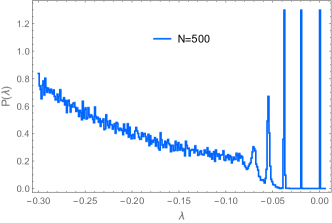
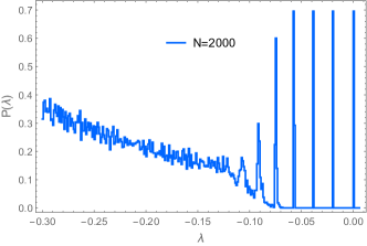
Figure 2: Probability density of the eigenvalues of $A^{\prime}$ for $\gamma=100$, computed for two system sizes. At larger $N$ one sees more isolated eigenvalues.

I.4.2 The spectrum of $F^{\prime}$

To estimate the eigenvalue distribution of $F^{\prime}$ we treat its off-diagonal elements as a perturbation. The diagonal elements are

$$-\frac{\gamma}{2}(\kappa_{i}-\kappa_{j})^{2}+i(H_{jj}-H_{ii})\equiv x_{ij}+iy_{ij}.\;\;\;\;\;\;\;\;\;\;\;\;\;\;\;(i\neq j).$$ (61)

Neglecting correlations between $\kappa_{i}$ and $\kappa_{j}$ we find that $x_{ij}$ is distributed according to

$$P(x_{ij})=\sqrt{\frac{2}{\gamma|x_{ij}|}}f\left(\sqrt{\frac{2|x_{ij}|}{\gamma}}\right)\Theta(-x_{ij})\Theta(4\gamma+x_{ij}),$$ (62)

where $f(x)$ is given by Eq.(21), resulting in

$$\mu(x)=-\frac{\gamma}{2},\;\;\;\;\;\;\;\;\sigma(x)=\sqrt{\frac{3}{8}}\gamma.$$ (63)

Because of level repulsion Eq. (62) needs to be modified for $|x_{ij}|<\gamma/N^{2}$, where the linear $\kappa$-spacing distribution leads to $P(|x_{ij}|<\gamma/N^{2})\sim N/\gamma$. The imaginary part, $y_{ij}$, is normally distributed with

$$\mu(y)=0,\;\;\;\;\;\;\;\;\sigma(y)=\sqrt{\frac{2}{N}}.$$ (64)

Within second order perturbation theory the unperturbed eigenvalue $x_{ij}+iy_{ij}$ acquires a shift due to the coupling of the corresponding eigenstate $\rho_{ij}$ to $2(N-2)$ other states $\rho_{kl}$ with either $k=i$ or $l=j$. These couplings are of the form $iH_{jl}$, etc. As a result, the numerator of the corresponding perturbative term

$$\frac{-H_{jl}^{2}}{x_{ij}-x_{il}+i(y_{ij}-y_{il})}\equiv-\frac{\zeta_{ij{\>\!}il}}{x_{ij{\>\!}il}+iy_{ij{\>\!}il}},$$ (65)

is distributed according to

$$P_{\zeta}(\zeta)=\sqrt{\frac{N}{\pi}}\frac{1}{\sqrt{\zeta}}e^{-N\zeta}\,\Theta(\zeta).$$ (66)

To estimate the shift in the real part of the eigenvalue due to these terms

$$\Delta x_{ij}=-\sum_{k\neq i}\frac{x_{ij{\>\!}kj}}{x_{ij{\>\!}kj}^{2}+y_{ij{\>\!}kj}^{2}}\zeta_{ij{\>\!}kj}-\sum_{l\neq j}\frac{x_{ij{\>\!}il}}{x_{ij{\>\!}il}^{2}+y_{ij{\>\!}il}^{2}}\zeta_{ij{\>\!}il}\equiv\sum_{k\neq i}\xi_{ij{\>\!}kj}\zeta_{ij{\>\!}kj}+\sum_{l\neq j}\xi_{ij{\>\!}il}\zeta_{ij{\>\!}il}\equiv\sum_{k\neq i}\chi_{ij{\>\!}kj}+\sum_{l\neq j}\chi_{ij{\>\!}il},$$ (67)

we approximate the function $f(x)$ in Eq. (62) by a Gaussian with the same (zero) mean and (unit) standard deviation as those of $f(x)$. As a result, and after neglecting correlations between $x_{ij}$ and $x_{il}$, we obtain the following distribution of $x_{ij{\>\!}il}$

$$P(x)=\Theta(x)\int_{-\infty}^{0}dl\frac{e^{l/\gamma}}{\sqrt{-\pi\gamma l}}\frac{e^{(l-x)/\gamma}}{\sqrt{\pi\gamma(x-l)}}+\Theta(-x)\int_{-\infty}^{x}dl\frac{e^{l/\gamma}}{\sqrt{-\pi\gamma l}}\frac{e^{(l-x)/\gamma}}{\sqrt{\pi\gamma(x-l)}}=\frac{1}{\pi\gamma}K_{0}\left(\frac{|x|}{\gamma}\right).$$ (68)

Taking into account the effect of level repulsion modifies the behavior at small $x$ leading to $P(|x|<1/N^{2})\sim\ln(N)/\gamma$. Noticing that $y_{ij{\>\!}il}=H_{jj}-H_{ll}$ we conclude that it is normally distributed with $\mu(y)=0$ and $\sigma(y)=\sqrt{2/N}$. We then have for $\xi_{ij{\>\!}il}$

$$P_{\xi}(\xi) = \frac{N^{1/2}}{2\pi^{3/2}\gamma}\int_{-\infty}^{\infty}dxdy\,K_{0}\left(\frac{|x|}{\gamma}\right)e^{-Ny^{2}/4}\delta\left(\xi+\frac{x}{x^{2}+y^{2}}\right)$$ (69)

$$= \frac{N^{1/2}}{2\pi^{3/2}\gamma}\frac{1}{|\xi|^{3}}\int_{-\infty}^{\infty}dy\frac{1}{(1+y^{2})^{2}}K_{0}\left[\frac{1}{\gamma|\xi|(1+y^{2})}\right]e^{-Ny^{2}/[4\xi^{2}(1+y^{2})^{2}]},$$

which leads to the approximate behaviour

$$P_{\xi}(\xi)\sim\left\{\begin{array}[]{cc}\frac{N^{1/2}}{\gamma}|\xi|^{-3}&\;\;\;\;\;\;|\xi|>N^{1/2}\\ \frac{1}{\gamma}|\xi|^{-2}&\;\;\;\;\;\;N^{1/2}>|\xi|>\gamma^{-1}\\ \frac{1}{\gamma N}&\;\;\;\;\;\;\gamma^{-1}>|\xi|\end{array}\right..$$ (70)

Using Eqs. (66) and (70) we arrive at the distribution for $\xi_{ij{\>\!}il}$

$$P_{\chi}(\chi)=\int_{0}^{\infty}d\zeta\,\frac{1}{\zeta}P_{\zeta}(\zeta)P_{\xi}\left(\frac{\chi}{\zeta}\right)\sim\left\{\begin{array}[]{cc}\frac{1}{\gamma N^{3/2}}|\chi|^{-3}&\;\;\;\;\;\;|\chi|>\frac{1}{N^{1/2}}\\ \frac{1}{\gamma N}|\chi|^{-2}&\;\;\;\;\;\;\frac{1}{N^{1/2}}>|\chi|>\frac{1}{\gamma N}\\ \gamma^{1/2}N^{1/2}|\chi|^{-1/2}&\;\;\;\;\;\;\frac{1}{\gamma N}>|\chi|\end{array}\right..$$ (71)

Once again, there is some numerical evidence that the decay in the range $1/N^{1/2}>|\chi|>1/(\gamma N)$ is slightly slower than $|\chi|^{-2}$ leading to $\mu(|\chi|)\sim 1/(\gamma N)$. For states near the upper edge of the $x_{ij}$ distribution almost all of $x_{ij{\>\!}il}=x_{ij}-x_{il}$ are positive, and thus almost all of the $2(N-2)$ perturbative corrections to the real part of their eigenvalue are negative, see Eq. (67). Consequently, the edge of the $x_{ij}$ distribution is shifted from zero by an amount of order $-1/\gamma$. Numerically we find that for large $N$ the prefactor of the shift is larger than 2 and that the first few eignevalues with the smallest real part (in terms of magnitude) come from the spectrum of $A^{\prime}$.

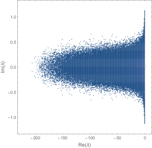
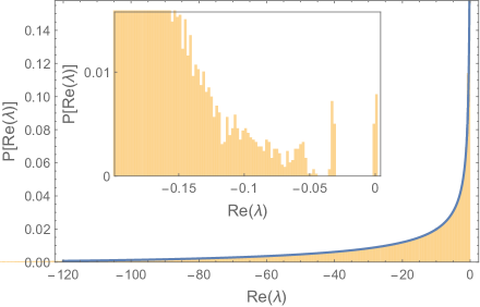
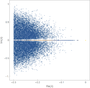
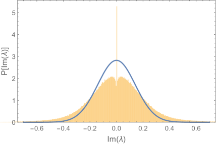
Figure 3: Left: Eigenvalues distribution of $\mathcal{L}$, calculated from averaging over 60 realizations for the case $\gamma=50$ and $N=100$. The lower panel depicts in more details the distribution near the origin. Right: The upper panel contains the projection of the distribution on the real axis. The blue line corresponds to Eq. (62) and the inset depicts the edge of the distribution. Note the isolated state between the edge of the eigenvalue cloud and the zero-mode at the origin. The lower panel shows the projection of the distribution on the imaginary axis alongside a normal distribution with standard deviation $\sqrt{2/N}$. The latter corresponds to the distribution of diagonal (unperturbed) elements of $\mathcal{L}$, and its deviation from the exact result is due to eigenvalues with small real parts [it fits the data reasonably well for $\rm{Re}(\lambda)<-10$]. In the $N\rightarrow\infty$ limit we expect that the standard deviations of the real and imaginary parts scale with $\gamma$ and $1/\gamma$, respectively.

For the shift in the imaginary part

$$\Delta y_{ij}=\sum_{k\neq i}\frac{y_{ij{\>\!}kj}}{x_{ij{\>\!}kj}^{2}+y_{ij{\>\!}kj}^{2}}\zeta_{ij{\>\!}kj}+\sum_{l\neq j}\frac{y_{ij{\>\!}il}}{x_{ij{\>\!}il}^{2}+y_{ij{\>\!}il}^{2}}\zeta_{ij{\>\!}il}\equiv\sum_{k\neq i}\eta_{ij{\>\!}kj}\zeta_{ij{\>\!}kj}+\sum_{l\neq j}\eta_{ij{\>\!}il}\zeta_{ij{\>\!}il}\equiv\sum_{k\neq i}\nu_{ij{\>\!}kj}+\sum_{l\neq j}\nu_{ij{\>\!}il}.$$ (72)

we need the distribution of $\eta_{ij{\>\!}il}$

$$P_{\eta}(\eta) = \frac{N^{1/2}}{2\pi^{3/2}\gamma}\int_{-\infty}^{\infty}dxdy\,K_{0}\left(\frac{|x|}{\gamma}\right)e^{-Ny^{2}/4}\delta\left(\eta-\frac{y}{x^{2}+y^{2}}\right)$$ (73)

$$= \frac{N^{1/2}}{2\pi^{3/2}\gamma}\frac{1}{|\eta|^{3}}\int_{-\infty}^{\infty}dx\frac{1}{(1+x^{2})^{2}}K_{0}\left[\frac{|x|}{\gamma|\xi|(1+x^{2})}\right]e^{-N/[4\xi^{2}(1+x^{2})^{2}]},$$

which can be approximated by

$$P_{\eta}(\eta)\sim\left\{\begin{array}[]{cc}\frac{N^{1/2}}{\gamma}|\eta|^{-3}&\;\;\;\;\;\;|\eta|>N^{1/2}\\ \frac{1}{\gamma N^{1/4}}|\eta|^{-3/2}&\;\;\;\;\;\;N^{1/2}>|\eta|>\frac{1}{\gamma^{2}N^{1/2}}\\ \gamma^{2}N^{1/2}&\;\;\;\;\;\;\frac{1}{\gamma^{2}N^{1/2}}>|\eta|\end{array}\right.$$ (74)

and thus the distribution of the correction $\nu_{ij{\>\!}il}$ is

$$P_{\nu}(\nu)=\int_{0}^{\infty}d\zeta\,\frac{1}{\zeta}P_{\zeta}(\zeta)P_{\eta}\left(\frac{\nu}{\zeta}\right)\sim\left\{\begin{array}[]{cc}\frac{1}{\gamma N^{3/2}}|\nu|^{-3}&\;\;\;\;\;\;|\nu|>\frac{1}{N^{1/2}}\\ \frac{1}{\gamma N^{3/4}}|\nu|^{-3/2}&\;\;\;\;\;\;\frac{1}{N^{1/2}}>|\nu|>\frac{1}{\gamma^{2}N^{3/2}}\\ \gamma^{2}N^{3/2}&\;\;\;\;\;\;\frac{1}{\gamma^{2}N^{3/2}}>|\nu|\end{array}\right..$$ (75)

Using that Eq.(75) results in $\mu(|\nu|)\sim 1/(\gamma N)$ we may estimate the average shift in the imaginary part of the eigenvalues

$$\mu(\Delta y_{ij})\sim\mu(|\nu|)\Bigg{[}\sum_{k\neq i}{\rm sign}(\nu_{ij{\>\!}kj})+\sum_{l\neq j}{\rm sign}(\nu_{ij{\>\!}il})\Bigg{]}\sim\frac{1}{\gamma}{\rm erf}\left(\frac{y_{ij}}{2/\sqrt{N}}\right).$$ (76)

A similar approximation to the one taken after Eq. (33) leads then to the conclusion that the shifted imaginary parts $\tilde{y}_{ij}=y_{ij}+\Delta y_{ij}$ are normally distributed with $\mu(\tilde{y}_{ij})=0$ and $\sigma(\tilde{y}_{ij})$ that varies from $\sqrt{2/N}$ for $N\ll\gamma^{2}$ to $O(1/\gamma)$ for $N\gg\gamma^{2}$.

II Small-$|\lambda|$ tails in other ensembles

In the main text we argued that the probability density of small gaps should obey a universal formula depending on the size $N$, the number of dissipators $k$, and the random-matrix ensemble $\beta$. In the main text we verified these predictions for the Gaussian orthogonal ensemble with a single jump operator. Here, we provide numerical support for this formula for the Gaussian unitary ensemble (i.e., matrices with complex entries) and for the case with $k>1$ distinct jump operators. This numerical evidence is shown in Fig. 4: the naive predictions in the main text, based on counting independent random numbers, appear to work in all cases we have looked at. (We have also checked these results for the symplectic and Ginibre ensembles; these results will be presented elsewhere.)

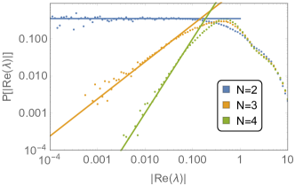
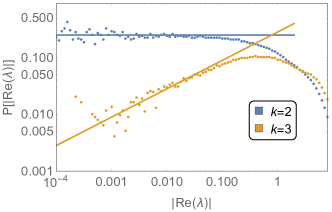
Figure 4: Left: density of states at small $|\lambda|$ for Hamiltonians and dissipators chosen from the Gaussian unitary ensemble, for $\gamma=2,k=1$. Right: Data for the Gaussian orthogonal ensemble with $N=2$ and $k>1$ distinct jump operators. Straight lines indicate the exponents according to Eq. (5) in the main text.

References

• (1) D. H. Carlson, On real eigenvalues of complex matrices, Pac. J. Math. 15, 1119 (1965).
• (2) E. M. Kessler, Generalized Schrieffer-Wolff formalism for dissipative systems, Phys. Rev. A 86, 012126 (2012).
• (3) W. Bryc, A. Dembo, T. Jiang, Spectral measure of large random Hankel, Markov and Toeplitz matrices, Annals of Prob. 34, 1 (2006).
• (4) C. Timm, Random transition-rate matrices for the master equation, Phys. Rev. E 80, 021140 (2009).