Testing extended Jordan-Brans-Dicke theories with future cosmological observations

Abstract

The extended Jordan-Brans-Dicke (eJBD) theory of gravity is constrained by a host of astrophysical and cosmological observations spanning a wide range of scales. The current cosmological constraints on the first post-Newtonian parameter in these simplest eJBD models in which the recent acceleration of the Universe is connected with the variation of the effective gravitational strength are consistent, but approximately two order of magnitude larger than the time-delay test within the Solar System. We forecast the capabilities of future galaxy surveys in combination with current and future CMB anisotropies measurements to further constrain the simplest dark energy models within eJBD theory of gravity. By considering two cases of a monomial potential (a quartic potential or a cosmological constant), we show how Euclid-like galaxy clustering and weak lensing data in combination with BOSS and future CMB observations have the potential to reach constraints on the first post-Newtonian parameter $\gamma_{\rm PN}$ comparable to those from the Solar System.

1 Introduction

Jordan-Brans-Dicke (JBD) theory of gravity [1, 2] is among the simplest extensions of general relativity (GR), in which the gravitational field is mediated by a scalar field whose inverse plays the role of an effective gravitational constant which varies in space and time. JBD theory depends on just one additional parameter $\omega_{\mathrm{BD}}$, connected to the post-Newonian parameter $\gamma_{\mathrm{PN}}=(1+\omega_{\mathrm{BD}})/(2+\omega_{\mathrm{BD}})$ measuring the deviations from Einstein GR, which is recovered in the limit of $\gamma_{\mathrm{PN}}\rightarrow 1$, i.e. $\omega_{\mathrm{BD}}\rightarrow+\infty$. Observations on a wide range of scales constrain JBD theory around GR: the tightest limits, $\gamma_{\mathrm{PN}}-1=(2.1\pm 2.3)\times 10^{-5}$ (68% CL) are obtained from radar timing data by the Cassini spacecraft within our Solar System [3].

Extended JBD (eJBD) theory of gravity with a potential term for the scalar field:

$${\cal S}=\int d^{4}x\sqrt{-g}\,\left[\frac{1}{16\pi}\left(\phi R-\frac{\omega_{\mathrm{BD}}}{\phi}g^{\mu\nu}\partial_{\mu}\phi\partial_{\nu}\phi\right)-V(\phi)+\mathcal{L}_{\rm m}\right]\,,$$ (1.1)

include the simplest scalar-tensor models of dark energy in which the current acceleration of the Universe is connected to a variation of the effective gravitational constant [4, 5, 6, 7, 8, 9, 10] (see also Ref. [11]). These models are also known as extended quintessence [6, 9].

The phenomenology in the eJBD theory of gravity is much richer than in Einstein Gravity (EG), since cosmological variation of the effective gravitational constant could lead to different predictions not only for cosmic microwave background (CMB) anisotropy [12] and the growth of structures, but also for Big Bang Nucleosynthesis (BBN) [13, 14].

Testing the viability of the cosmology in eJBD theory is fully complementary to the Solar System constraints just presented. For models described by Eq. (1.1) with a quadratic potential [11, 4, 15], the recent $Planck$ 2015 [16, 17] and baryonic acoustic oscillations (BAO) data [18, 19, 20] constrain $1-\gamma_{\mathrm{PN}}<0.003$ (95% CL) [21] (see also [22] for constraints obtained by relaxing the hypothesis of flat spatial sections and [23, 24, 25] for the constraints based on the $Planck$ 2013 data). These cosmological constraints on $\gamma_{\rm PN}$ are approximately two order of magnitude looser than Solar System constraints.

In this paper we investigate the capabilities of future CMB and large scale structures (LSS) observations to further improve the cosmological constraints on the post-Newtonian parameter $\gamma_{\rm PN}$ within the eJBD theory, as also forecasted in [26, 27]. We expect that upcoming galaxy surveys such as DESI [28], Euclid [29, 30], LSST [31], SKA [32, 33], will help in improving the constraints of structure formation on $\gamma_{\rm PN}$ for the eJBD theory. As a representative example of what we will gain from upcoming galaxy surveys, we consider the two main probes of Euclid, galaxy clustering (GC), and weak lensing (WL). In addition, we will consider the role of possible future CMB polarization anisotropy observations, as AdvACT [34], CORE [35, 36, 37], LiteBIRD [38, 39], and S4 [40], in further improving on the $Planck$ measurements.

Our paper is organized as follows. After this introduction, we give a lighting review of eJBD recast as Induced Gravity (IG) (by a redefinition of the scalar field with standard units and standard kinetic term) in Section 2. In Section 3 and 4 we present the Fisher methodology for CMB and LSS for our science forecasts. In Section 5 we present our results and in Section 6 we draw our conclusions.

2 Dark Energy within the extended Jordan-Brans-Dicke theories

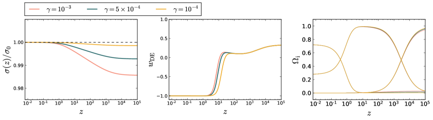
Figure 1: Evolution of $\sigma/\sigma_{0}$ (top panel), $w_{\rm DE}$ (middle panel), and $\Omega_{i}$ (bottom panel) as function of $z$ for different choices of $\gamma$ from $\gamma=10^{-4}$ to $\gamma=10^{-3}$ for $n=4$. The value $\sigma_{0}$ of the scalar field at present is fixed consistently with the Cavendish-type measurement of the gravitational constant $G=6.67\times 10^{-8}$ cm³ g^-1 s^-2.

In this section we review some general considerations of the late-time cosmology within the eJBD theories.

We consider a field redefinition to recast the eJBD action in Eq. (1.1) into an action for induced gravity (IG) with a standard kinetic term for a scalar field $\sigma$:

$$\mathcal{S}=\int d^{4}x\sqrt{-g}\left[\frac{\gamma\sigma^{2}R}{2}-\frac{g^{\mu\nu}}{2}\partial_{\mu}\sigma\partial_{\nu}\sigma-V(\sigma)+\mathcal{L}_{\mathrm{m}}\right]\,.$$ (2.1)

where $\gamma=(4\omega_{\mathrm{BD}})^{-1}$ and $\gamma\sigma^{2}=\phi$.

The cosmology evolution after inflation can be divided roughly in three stages and is summarized in Fig. 1. In the first stage relevant for our study, i.e. deep in the radiation era, $\sigma$ is almost frozen, since it is effectively massless and non-relativistic matter is subdominant. During the subsequent matter dominated era, $\sigma$ is driven by non-relativistic matter to higher values, leading to an effective gravitational constant $G_{\rm N}(a)=1/\left(8\pi\gamma\sigma^{2}\right)$ which decrease in time. The potential $V(\sigma)$ kicks in only at recent times determining the rate of the accelerated expansion. For a simple monomial potential $V(\sigma)\propto\sigma^{n_{\rm IG}}$ and in absence of matter, exact power-law solutions for the scale factor $a(t)\sim t^{p}$ describing an accelerated expansion exist for the class of monomial potentials with $p=2\frac{1+(n_{\rm IG}+2)\gamma}{(n_{\rm IG}-4)(n_{\rm IG}-2)\gamma}$ [41, 42]. A de Sitter solution for the scale factor is found instead for $n_{\rm IG}=2\,,4$.

In Fig. 1 we display different quantities as a function of redshift: the scalar field normalized to its value at present (left panel), the parameter of state $w_{\mathrm{DE}}$ of the effective dark energy component (middle panel), and the critical densities corresponding to EG with a gravitational constant given by the current value of the scalar field, i.e. $8\pi G_{\rm N}(z=0)=1/(\gamma\sigma_{0}^{2})$. It is interesting to note from $w_{\mathrm{DE}}$ displayed in Fig. 1 that the effective parameter of state for dark energy in these extended JBD models is similar to the so called old [43] and new [44] early dark energy models.

Since now on we will restrict ourselves to two cases of monomial potentials, i.e. $V(\sigma)\propto\sigma^{n_{\rm IG}}$ with $n_{\rm IG}=4$ or $n_{\rm IG}=0$, suitable to reproduce a background cosmology in agreement with observations. We consider a scalar field $\sigma=\sigma_{i}$ nearly at rest deep in the radiation era, since an initial non-vanishing time derivative would be otherwise rapidly dissipated [15]. The initial time derivative of the scalar field is taken as $d\sigma/\mathrm{d}\tau=3\gamma\omega\sigma_{i}/2$ - with $\omega=\frac{\rho_{m\,0}}{\sqrt{3\gamma\rho_{r\,0}}(1+6\gamma)\sigma_{i}}$ - satisfying the equation of motion. We choose $\sigma_{i}$ by fixing the value $\sigma_{0}$ of the scalar field at present consistently with the Cavendish-type measurement of the gravitational constant $G=6.67\times 10^{-8}$ cm³ g^-1 s^-2, i.e. $\gamma\sigma_{0}^{2}=\frac{1}{8\pi G}\frac{1+8\gamma}{1+6\gamma}$. We also consider adiabatic initial conditions for fluctuations [45]. In this way for a given potential the models we study have just one parameter in addition to the $\Lambda$CDM model, i.e. the coupling to the Ricci curvature $\Lambda$CDM model $\gamma$.

The evolution of linear perturbations in this class of eJBD can be described with a set of dimensionless functions $\alpha_{\rm M}=\mathrm{d}\ln\phi/\mathrm{d}\ln a$, $\alpha_{\rm B}=-\alpha_{\rm M}$, $\alpha_{\rm K}=\omega_{\rm BD}\alpha_{\rm M}^{2}$, and $\alpha_{\rm T}=0$ according to the parametrisation introduced in Ref. [46].

$Planck$ 2015 temperature, polarization and lensing [16, 17] constrain $\gamma<0.0017$ at 95% CL and by combining with BAO data the 95% CL upper bound tightens to $0.00075$ [21]. The cosmological variation of the effective gravitational strength between now respect to the one in the relativistic era is constrained as $|\delta G_{N}/G_{N}|<0.039$ at 95% CL [21]. Such eJBD models predict a value for the Hubble parameter larger than $\Lambda$CDM, because of a degeneracy between $\gamma$ and $H_{0}$. This effect can be easily understood by interpreting the larger value of the effective gravitational constant in the past as a larger number of relativistic degrees of freedom.

Constraints on $\gamma$ and $\delta G_{N}/G_{N}$ based on current CMB and BAO data do not depend significantly on the index of the monomial potential, but cosmological bounds on $\dot{G}_{N}/G_{N}$ do [21].

There is still cosmological information for eJBD models to extract from the CMB pattern beyond $Planck$. In Fig. 2, it shows the residuals of the lensed TT and EE CMB angular power spectrum as function of the multipole $\ell$ with respect to the sample variance for a sky fraction of $f_{\rm sky}=0.7$ and $f_{\rm sky}=0.4$. Note the promise of E-mode polarization spectrum to constrain $\gamma$, we show the room of improvement on $\gamma$ expected from CMB temperature and polarization power spectra.

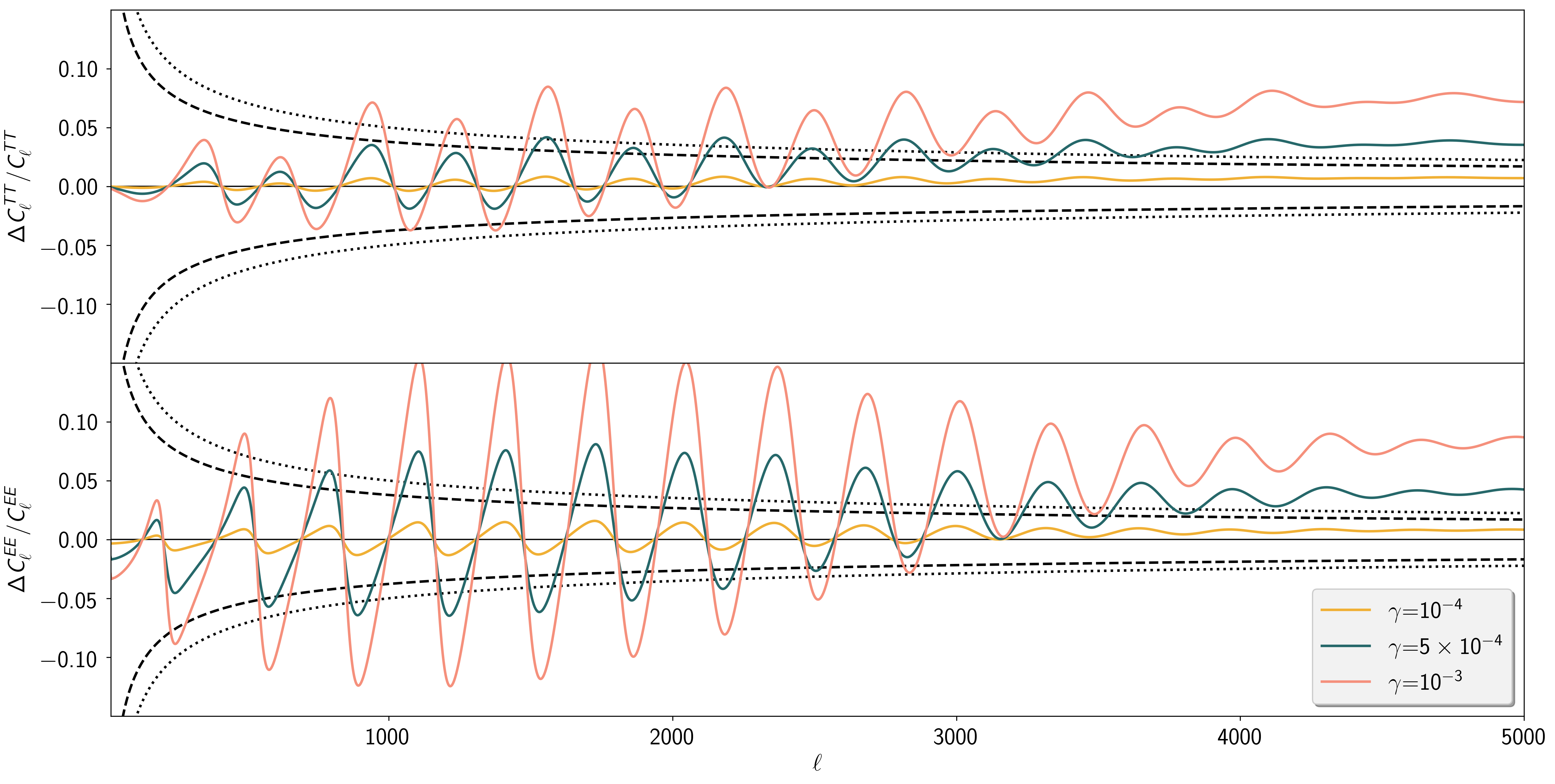
Figure 2: Relative change in the CMB angular power spectra induced by different values of the coupling parameter from $\gamma=10^{-4}$ to $\gamma=10^{-3}$. The black dashed (dotted) line refers to the noise spectrum of a cosmic-variance limited experiment with a sky fraction of $f_{\rm sky}=0.7\,(0.4)$.

3 Fisher approach for CMB anisotropy data

In this section, we start describing the formalism for our science forecasts. Under the Gaussian assumption for signal and noise, the Fisher matrix for CMB anisotropies in temperature and polarization [47, 48, 49, 50, 51] is:

$${\bf{\rm F}}_{\alpha\beta}^{\rm CMB}=f_{\rm sky}\sum_{\ell}\frac{(2\ell+1)}{2}\sum_{\rm X,Y}\frac{\partial C_{\ell}^{\rm X}}{\partial\theta_{\alpha}}\left({\rm Cov}_{\ell}^{-1}\right)_{\rm XY}\frac{\partial C_{\ell}^{\rm Y}}{\partial\theta_{\beta}}\,,$$ (3.1)

where $C_{\ell}^{\rm X}$ is the CMB angular power spectrum in the $\ell^{\text{th}}$ multipole for X,Y $\in($TT$,\,$EE$,\,$TE$,\,\phi\phi,\,$T$\phi)$ , and $\theta_{\alpha}$ refers to the base of parameters considered in the analysis which are specified in Sec. 5 togheter with their best-fit value. The elements of the symmetric angular power spectrum covariance matrix $\text{Cov}_{\ell}$ at the $\ell^{\text{th}}$ multipole are:

$$\left({\rm Cov}_{\ell}\right)_{\rm TTTT} =\left(\bar{C}_{\ell}^{\rm TT}\right)^{2}-2\frac{\left(\bar{C}_{\ell}^{\rm TE}\bar{C}_{\ell}^{\rm T\phi}\right)^{2}}{\bar{C}_{\ell}^{\rm EE}\bar{C}_{\ell}^{\rm\phi\phi}}\,,$$ (3.2)

$$\left({\rm Cov}_{\ell}\right)_{\rm EEEE} =\left(\bar{C}_{\ell}^{\rm EE}\right)^{2}\,,$$ (3.3)

$$\left({\rm Cov}_{\ell}\right)_{\rm TETE} =\frac{\left(\bar{C}_{\ell}^{\rm TE}\right)^{2}+\bar{C}_{\ell}^{\rm TT}\bar{C}_{\ell}^{\rm EE}}{2}-\frac{\bar{C}_{\ell}^{\rm EE}\left(\bar{C}_{\ell}^{\rm T\phi}\right)^{2}}{2\bar{C}_{\ell}^{\rm\phi\phi}}\,,$$ (3.4)

$$\left({\rm Cov}_{\ell}\right)_{\rm\phi\phi\phi\phi} =\left(\bar{C}_{\ell}^{\rm\phi\phi}\right)^{2}\,,$$ (3.5)

$$\left({\rm Cov}_{\ell}\right)_{\rm T\phi T\phi} =\frac{\left(\bar{C}_{\ell}^{\rm T\phi}\right)^{2}+\bar{C}_{\ell}^{\rm TT}\bar{C}_{\ell}^{\phi\phi}}{2}-\frac{\bar{C}_{\ell}^{\phi\phi}\left(\bar{C}_{\ell}^{\rm TE}\right)^{2}}{2\bar{C}_{\ell}^{\rm EE}}\,,$$ (3.6)

$$\left({\rm Cov}_{\ell}\right)_{\rm TTEE} =\left(\bar{C}_{\ell}^{\rm TE}\right)^{2}\,,$$ (3.7)

$$\left({\rm Cov}_{\ell}\right)_{\rm TTTE} =\bar{C}_{\ell}^{\rm TT}\bar{C}_{\ell}^{\rm TE}-\frac{\bar{C}_{\ell}^{\rm TE}\left(\bar{C}_{\ell}^{\rm T\phi}\right)^{2}}{\bar{C}_{\ell}^{\phi\phi}}\,,$$ (3.8)

$$\left({\rm Cov}_{\ell}\right)_{\rm TT\phi\phi} =\left(\bar{C}_{\ell}^{\rm T\phi}\right)^{2}\,,$$ (3.9)

$$\left({\rm Cov}_{\ell}\right)_{\rm TTT\phi} =\bar{C}_{\ell}^{\rm TT}\bar{C}_{\ell}^{\rm T\phi}-\frac{\bar{C}_{\ell}^{\rm T\phi}\left(\bar{C}_{\ell}^{\rm TE}\right)^{2}}{\bar{C}_{\ell}^{\rm EE}}\,,$$ (3.10)

$$\left({\rm Cov}_{\ell}\right)_{\rm EETE} =\bar{C}_{\ell}^{\rm EE}\bar{C}_{\ell}^{\rm TE}\,,$$ (3.11)

$$\left({\rm Cov}_{\ell}\right)_{\rm\phi\phi T\phi} =\bar{C}_{\ell}^{\phi\phi}\bar{C}_{\ell}^{\rm T\phi}\,,$$ (3.12)

where $\bar{C}_{\ell}^{\rm X}=C^{\rm X}_{\ell}+N^{\rm X}_{\ell}$ is the sum of the signal and the noise, with $N^{\rm TE}_{\ell},N^{\rm T\phi}_{\ell}=0$. For the temperature and polarization angular power spectra, here $N^{\rm X}_{\ell}=\sigma_{\rm X}b^{-2}_{\ell}$ is the isotropic noise convolved with the instrument beam, $b_{\ell}^{2}$ is the beam window function, assumed Gaussian, with $b_{\ell}=e^{-\ell(\ell+1)\theta_{\rm FWHM}^{2}/16\ln 2}$; $\theta_{\rm FWHM}$ is the full width half maximum (FWHM) of the beam in radians; $w_{\rm TT}$ and $w_{\rm EE}$ are the inverse square of the detector noise level on a steradian patch for temperature and polarization, respectively. For multiple frequency channels, $\sigma^{-1}_{\rm X}b_{\ell}^{2}$ is replaced by sum of this quantity for each channels [47]:

$$N^{\rm X}_{\ell}=\left[\sum_{\rm channels}\frac{1}{N^{\rm X}_{\rm\ell,i}}\right]^{-1}\,.$$ (3.13)

We consider the minimum variance estimator for the noise of the lensing potential by combining the TT, EE, BB, TE, TB, EB CMB estimators calculated according to [52].

In this paper, we consider four different cases as representative of current CMB measurements and future concepts. We study the predictions for a $Planck$-like experiment consideridering the specifications of $f_{\rm sky}=0.7$, and a multipole range from $\ell_{\rm min}=2$ up to $\ell_{\rm max}=2500$ in Eq. (3.1). We use one cosmological frequency of 143 GHz assuming in flight performace corresponding to a sensitivity of $33\,\mu$K-arcmin in temperature and $70.2\,\mu$K-acmin in polarization, with a Gaussian beam width of 7.3 arcmin [53], see CMB-1 in [54].

Since small-scale CMB anisotropy measurements will improve thanks to Stage-3 generation of ground-based CMB experiments, we consider AdvACT [34, 55] with a noise level of $1.4\,\mu$K-arcmin in temperature and $8\,\mu$K-acmin in polarization, with a Gaussian beam width of 1.4 arcmin and $f_{\rm sky}=0.4$, over a multipole range $30\leq\ell\leq 3000$.

As concept for the next generation of CMB polarization experiments, we consider CORE and Stage-4 (hereafter S4). For CORE, we consider six frequency channels between 130 and 220 GHz with noise sensitivities of $1.5\,\mu$K-arcmin in temperature and $2\,\mu$K-acmin in polarization, with a Gaussian beam width of 5.5 arcmin [35, 36, 37]. We consider $\ell_{\rm max}=3000$ for the CORE configuration with a sky coverage of $f_{\rm sky}=0.7$.

The ground-based S4 proposal will be able to map modes up to $\ell\sim 5000$. Following [40], we consider for S4 a sensitivity $\sigma_{\rm T}=\sigma_{\rm P}/\sqrt{2}=1\,\mu$K-arcmin with a resolution of $\theta_{\rm FWHM}=3$ arcmin over $\sim 40\%$ of the sky. Ground-based facilities are limited on large scales due to galactic foreground contamination and in addition a contamination is expected on the small scales in temperature. For these reasons, we assume for S4 $\ell_{\rm min}=30$ and a different cut at high-$\ell$ of $\ell_{\rm max}^{\rm T}=3000$ in temperature and $\ell_{\rm max}^{\rm P}=5000$ in polarization. To complement at low multipoles, i.e. $2\leq\ell<30$, we combine with $Planck$ AdvACT and with the Japan CMB polarization space mission proposal LiteBIRD [38, 39] S4. For the estimate of the noise of the lensing potential we use the multipole range $30\leq\ell\leq 3000$.

4 Fisher approach for LSS data

We now give the details for the Fisher forecasts with future LSS data. We consider Euclid-like specifications as a representative case for future galaxy surveys. Euclid is a mission of the ESA Cosmic Vision program that it is expected to be launched in 2022. It will perform both a spectroscopic and a photometric survey: the first aims mainly at measuring the galaxy power spectrum of $\sim 30,000,000$ galaxies while the second at measuring the weak lensing signal by imaging $\sim 1.5$ billion galaxies.

Both surveys will be able to constrain both the expansion and growth history of the universe and will cover a total area of $15,000$ square degrees.

4.1 Spectroscopic galaxy power spectrum

Following [56], we write the linear observed galaxy power spectrum as:

$$P_{gal}(z:k_{r},\mu_{r})=\frac{D_{Ar}^{2}(z)H(z)}{D_{A}^{2}(z)H_{r}(z)}\left[b(z)\sigma_{8}(z)+f(z,\,k)\sigma_{8}(z)\mu^{2}\right]^{2}\frac{P_{r}(z,\,k)}{\sigma_{8}^{2}(z)}+P_{\mathrm{shot}}(z)\,,$$ (4.1)

where the subscript $r$ refers to the reference (or fiducial) cosmological model.

Here $P_{\mathrm{shot}}(z)$ is a scale-independent offset due to imperfect removal of shot-noise, $\mu\equiv\vec{k}\cdot\hat{r}/k$ is the cosine of the angle of the wave mode with respect to the line of sight pointing into the direction $\hat{r}$, $P_{r}(z,\,k)$ is the fiducial matter power spectrum evaluated at different redshifts, $b(z)$ is the bias factor, $f(z,\,k)$ is the growth rate, $H(z)$ is the Hubble parameter and $D_{A}(z)$ is the angular diameter distance. The wavenumber $k$ and $\mu$ have also to be written in terms of the fiducial cosmology (see for more details [56, 57, 58]). The fiducial bias used in this paper is $b(z)=0.72z+0.7$ according to [59].

The Fisher matrix for the galaxy power spectrum is given by [56]:

$$F_{\alpha\beta}=\int_{k_{\text{min}}}^{k_{\text{max}}}\frac{k^{2}\mathrm{d}k}{4\pi^{2}}\frac{\partial\ln P_{gal}(z;\,k,\mu)}{\partial\theta_{\alpha}}\frac{\partial\ln P_{gal}(z;\,k,\mu)}{\partial\theta_{\beta}}\times V_{\text{eff}}\,.$$ (4.2)

The observed galaxy power spectrum is given by Eq. (4.1) and the derivatives are evaluated numerically at the fiducial cosmology; $k_{\text{min}}=0.001\,h/\text{Mpc}$ and its value depends on the survey size whereas $k_{\text{max}}$ is such that root mean square amplitude of the density fluctuations at the scale $R_{\text{max}}=2\pi/k_{\text{max}}\,\text{Mpc}/h$ is $\sigma^{2}(R_{\text{max}})=0.25$, however in order to not depend strongly on the non-linear information we consider two cases imposing an additional cut at $k_{\text{max}}=0.1\,h/\text{Mpc}$ and at $k_{\text{max}}=0.25\,h/\text{Mpc}$. The effective volume of the survey in each bin is given by:

$$V_{\text{eff}}=\left(\frac{\bar{n}\,P_{gal}(z;\,k,\mu)}{1+\bar{n}\,P_{gal}(z;\,k,\mu)}\right)^{2}V_{\text{survey}}\,,$$ (4.3)

where $\bar{n}$ is the average comoving number density in each bin, the value of the $\bar{n}$ and fiducial specific Euclid-like specifications can be found in [60, 61].

To complete the GC information, we include low-redshift spectroscopic information from BOSS [62, 63] on the redshift range $0.2<z<0.8$ over 10,000 square degrees.

4.2 Weak Lensing

The weak lensing convergence power spectrum is given by [64, 65, 66, 67, 68]:

$$P_{ij}(\ell)=H_{0}^{3}\int_{0}^{\infty}\frac{\mathrm{d}z}{E(z)^{2}}\>W_{i}(z)W_{j}(z)\>P_{\mathrm{NL}}\left(k=\frac{H_{0}\,\ell}{r(z)},z\right)\,,$$ (4.4)

where the subscript ${ij}$ refers to the redshift bins around $z_{i}$ and $z_{j}$, with $W_{i}(z)$ is the window function (see [69] for more details). The tomographic overall radial distribution function of galaxies for a Euclid-like photometric survey is [30]:

$$D(z)=z^{2}\exp\left[-\left(z/z_{0}\right)^{1.5}\right]\,.$$ (4.5)

with $z_{0}=z_{\text{mean}}/1.412$ and mean redshift $z_{\text{mean}}=0.9$, the number density is $d=35\text{ galaxy per arcmin}^{2}$. Moreover we consider a survey up to $z_{\text{max}}=3$ divided into 10 bins each containing the same number of galaxies. While tomography in general greatly reduces statistical errors the actual shape of the choice of the binning does not affect results in a serious way, although in principle there is room for optimisation [70].

The Fisher matrix for weak lensing is defined as:

$$F_{\alpha\beta}=f_{\text{sky}}\sum_{\ell}\frac{(2\ell+1)\Delta\ell}{2}\frac{\partial P_{i\,j}}{\partial\theta_{\alpha}}C_{j\,k}^{-1}\frac{\partial P_{k\,m}}{\partial\theta_{\beta}}C_{m\,i}^{-1}\,,$$ (4.6)

where $\Delta\ell$ is the step in multipoles, to which we chose 100 step in logarithm scale; whereas $\theta_{\alpha}$ are the cosmological parameters and:

$$C_{j\,k}=P_{j\,k}+\delta_{j\,k}\langle\gamma_{\text{int}}^{2}\rangle\,n_{j}^{-1}\,,$$ (4.7)

where $\gamma_{\text{int}}$ is the rms intrinsic shear, which is assumed $\langle\gamma_{\text{int}}^{2}\rangle^{1/2}=0.22$. The number of galaxies per steradians in each bin is defined as:

$$n_{j}=3600\,d\left(\frac{180}{\pi}\right)^{2}\hat{n}_{j}\,,$$ (4.8)

where $d$ is the number of galaxies per square arcminute and $\hat{n}_{j}$ is the faction of sources that belongs to the $j-$th bin.

5 Statistical errors forecasts

In this section we estimate marginalised statistical errors for the cosmological parameters of our model, using the Fisher matrix calculation. The probes are assumed to be independent, hence the total Fisher matrix is simply given by the sum of the single Fisher matrices:

$$F_{\alpha\beta}=F_{\alpha\beta}^{\text{CMB}}+F_{\alpha\beta}^{\text{GC}}+F_{\alpha\beta}^{\text{WL}}\,.$$ (5.1)

We perform the Fisher forecast analysis for the set of parameters $\omega_{\rm c},{\bf\theta}=\{\omega_{\rm b},h_{0},n_{\rm s},\ln(10^{10}A_{\rm s}),\gamma\}$. For the CMB we consider also the reionization optical depth $\tau$ and then we marginalize over it before to combine the CMB Fisher matrix with the other two. We assume as fiducial model a flat cosmology with best-fit parameters corresponding to $\omega_{\textrm{c}}\equiv\Omega_{\textrm{c}}h^{2}=0.1205$, $\omega_{\textrm{b}}\equiv\Omega_{\textrm{b}}h^{2}=0.02218$, $h_{0}\equiv H_{0}/100=0.6693$, $\tau=0.0596$, $n_{\textrm{s}}=0.9619$, and $\ln\left(10^{10}\ A_{\textrm{s}}\right)=3.056$ consistent with the recent results of $Planck$ [71]. As a fiducial value for the coupling to the Ricci curvature we choose $\gamma=10^{-5}$, the value is within the 95% CL upper bound from current cosmological data [21] and is contrained at 3$\sigma$ with the Solar System data [3]. We have considered two fiducial potentials, a quartic potential and a constant one.

The CMB angular power spectra, the matter power spectra, together with the Hubble parameter $H(z)$, the angular diameter distance $D_{A}(z)$, and growth rate $f(z,k)$ have been computed with CLASSig, a modified version of the Einstein-Boltzmann code CLASS [72, 73] dedicated to eJBD theory [25]. This code has been successfully validated against other codes in [74]. Non-linear scales have been included to the matter power spectrum assuming the halofit model from [75].

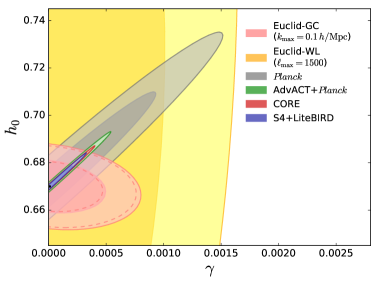
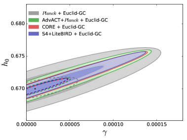
Figure 3: Left: joint marginalized constraints (68%-95% CL) on $h_{0}$ and $\gamma$ from single probe alone. Dashed lines correspond to the 68%-95% CL using the GC information from Euclid-like in combination with BOSS. Right: joint marginalized constraints (68%-95% CL) on $h_{0}$ and $\gamma$ from the combination CMB+Euclid-GC for the four CMB surveys. Dashed lines correspond to the 68% CL using the GC information up to $k_{\rm max}=0.25\,h/\text{Mpc}$.

Fig. 3 shows the constraints from the single observational probes. The different orientation of the 2-dimensional contours shows that the most efficient way to reduce the constraint error on $\gamma$ is to combine different cosmological probes.
With our Fisher approach, we find that the uncertainty from $Planck$ simulated data alone is $\sigma(\gamma)\simeq 0.00064$ at 68% CL (consistent with our finding with $Planck$ 2015 real data [21]) will improve by a factor three using AdvACT+$Planck$, a factor four with CORE, and a factor five with the combination S4+LiteBIRD, i.e. $\sigma(\gamma)\simeq 0.00022,\,0.00016,\,0.00013$ at 68% CL respectively.

The combination of quasi-linear information with $k_{\rm max}=0.1\,h/\text{Mpc}$ from galaxy GC spectrum from Euclid-like and BOSS to the CMB leads to a significant improvement of the uncertainty on $\gamma$, approximately three-ten times with respect to the constraints obtained with the CMB alone.

In order to understand the improvement carried by mildly non-linear scales, we also include the case of $k_{\rm max}=0.25\,h/\text{Mpc}$ which further improves the uncertainty on $\gamma$. In this case, we find five-twenty times better errors compared to CMB alone. We show in Fig. 3 the 2-dimensional marginal errors for the combination of CMB+Euclid-GC Fisher matricies for $Planck$, AdvACT+$Planck$, CORE, S4+LiteBIRD which correspond to the uncertainties of $\sigma(\gamma)\simeq 0.000058\,(0.000032)$, $\sigma(\gamma)\simeq 0.000054\,(0.000027)$, $\sigma(\gamma)\simeq 0.000052\,(0.000025)$, $\sigma(\gamma)\simeq 0.000051\,(0.000025)$ at 68% CL for $k_{\rm max}=0.1\,(0.25)\,h/\text{Mpc}$; including also BOSS-GC information we obtain respectively $0.000057\,(0.000031)$, $0.000052\,(0.000026)$, $0.000050\,(0.000024)$, $0.000049\,(0.000023)$ at 68% CL for $k_{\rm max}=0.1\,(0.25)\,h/\text{Mpc}$.

Finally, we considered the combination of our three cosmological probes (CMB, GC, WL) to identify the tightest constraint on $\gamma$ by including non-linear scales through WL. The sensitivity on $\gamma$ combining the CMB with GC information up to $k_{\rm max}=0.1\,h/\text{Mpc}$ and WL assuming $\ell_{\rm max}=1500$ corresponds to $\sigma(\gamma)\simeq 0.000045$, $\sigma(\gamma)\simeq 0.000037$, $\sigma(\gamma)\simeq 0.000029$, $\sigma(\gamma)\simeq 0.000023$, at 68% CL for $Planck$, AdvACT+$Planck$, CORE, and S4+LiteBIRD. These uncertainties improve of another 1.5 factor if we push the GC information up to $k_{\rm max}=0.25\,h/\text{Mpc}$.

We show in Fig. 4 the impact of non-linear scales pushing the WL up to our optimistic case of $\ell_{\rm max}=5000$. We find a small improvement in terms of error on $\gamma$ pushing $\ell_{\rm max}$ for the WL from 1500 to 5000.

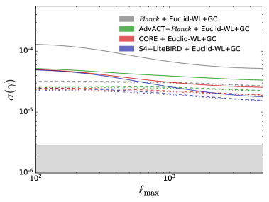
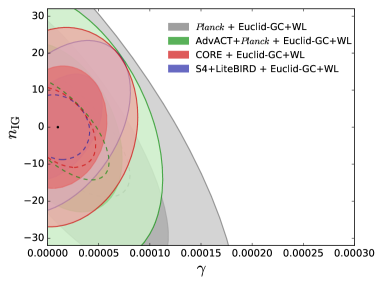
Figure 4: Left: forecast marginalized constraint on $\gamma$ (68% CL) as a function of the maximum multipole $\ell_{\rm max}$ included in the WL. Dashed lines correspond to the combination GC using the Euclid-GC information up to $k_{\rm max}=0.25\,h/\text{Mpc}$, and dot-dashed lines including also BOSS up to $k_{\rm max}=0.25\,h/\text{Mpc}$. The gray shaded region represent the 68% CL contraint from Solar System data [3]. Right: joint marginalized constraints (68%-95% CL) on $n_{\rm IG}$ and $\gamma$ from the combination CMB+Euclid-GC for the four CMB surveys. Dashed lines correspond to the 68% CL using the Euclid-GC information up to $k_{\rm max}=0.25\,h/\text{Mpc}$.

The most conservative forecast of Euclid-like plus BOSS to quasi-linear scales in combination with $Planck$ improve between a factor three and approximately a factor twenty the current uncertainties based on $Planck$ 2015 and BAO data.

In Tab. 1, we show the marginalized uncertainties on all the cosmological parameters from the combination of the CMB surveys with Euclid-like and BOSS using the conservative range of scales.

Table 1: Marginalized uncertainties (68% CL) on the cosmological parameters for $\gamma=10^{-5}$ and $n_{\rm IG}=4$. We consider the combination of three CMB surveys with the information up to quasi-linear scales from the GC ($k_{\rm max}=0.1\ h/$Mpc) using Euclid-like plus BOSS and WL ($\ell_{\rm max}=1500$) from Euclid-like. Numbers in round brakets refer to the uncertainties for our optimistic case with GC up to $k_{\rm max}=0.25\ h/$Mpc and WL up to $\ell_{\rm max}=5000$.

	$Planck$	AdvACT+$Planck$	S4+LiteBIRD
	+ BOSS-GC	+ BOSS-GC	+ BOSS-GC
	+ Euclid-GC+WL	+ Euclid-GC+WL	+ Euclid-GC+WL
$10^{4}~{}\sigma(\omega_{c})$	1.3 (1.1)	1.0 (0.78)	0.83 (0.67)
$10^{5}~{}\sigma(\omega_{b})$	9.8 (8.8)	4.5 (3.8)	3.2 (2.8)
$10^{3}~{}\sigma(h)$	1.7 (0.99)	1.4 (0.84)	1.0 (0.64)
$10^{3}~{}\sigma(n_{s})$	1.8 (1.2)	1.5 (0.96)	1.2 (0.88)
$10^{3}~{}\sigma\left(\ln\left(10^{10}A_{s}\right)\right)$	1.3 (0.75)	1.1 (0.71)	0.98 (0.56)
$10^{5}~{}\sigma(\gamma)$	4.5 (2.7)	3.7 (2.2)	2.3 (1.5)

We study the impact of a larger fiducial value for $\gamma=10^{-4}$ (still compatible with current $Planck$ 2015 + BAO constraints) on the forecasted uncertainties. We find that the effect on CMB and GC is around $\sim 10\%$ on the uncertainties; this implies that we will be able to detect at 2-5 $\sigma$ CL a value of $\gamma=10^{-4}$ with the combination of the CMB with GC information from a Euclid-like experiment. Regarding the WL, the uncertainties halve leading to a clearer detection of such $\gamma$ at more then 5 $\sigma$ when WL from Euclid-like is added.

We repeat our series of forecasts with a different potential for the scalar field with an index equal to zero, i.e. $n_{\rm IG}=0$, namely a cosmological constant. For this fiducial cosmology we find only a small degradation of the uncertainties on $\gamma$, pointing to a weak correlation between the two parameters.

Finally, we test also the possibility to constraint the index of the scalar potential around $n_{\rm IG}=0$ with future cosmological data, see Fig. 4. The tightest uncertainty that we obtain combining all the three cosmological probes and including non-linear scales in the GC up to $k_{\rm max}=0.25\,h/\text{Mpc}$ and in the WL up to $\ell_{\rm max}=5000$ is $\sigma\left(n_{\rm IG}\right)\simeq 5$ at 68% CL.

In order to compare our finding on cosmological scales with the constraints obtained within the Solar System we quote the constraint on the post-Newtonian parameters defined for this class of eJBD theories as:

$$\gamma_{\rm PN}=\frac{1+4\gamma}{1+8\gamma}\,.$$ (5.2)

Our derived forecasted uncertainties span between $\sigma\left(|\gamma_{\rm PN}-1|\right)\simeq 5.3\times 10^{-4}-2.5\times 10^{-3}$ at 68% CL for a CMB experiment with a $Planck$ sensitivity through a future CMB experiment able to perform a cosmic-variance measurement of the E-mode polarization at small scales. Combining CMB information with GC and WL, we find $\sigma\left(|\gamma_{\rm PN}-1|\right)\simeq 9.2\times 10^{-5}$ and including non-linear scales a minimum error on the deviation from GR in the weak field limit corresponding to $\sigma\left(|\gamma_{\rm PN}-1|\right)\simeq 6.2\times 10^{-5}$ at 68% CL.

6 Conclusion

eJBD theories represent the simplest scalar-tensor theory of gravity where Newton’s constant is allow to vary becoming a dynamical field, as a function of space and time.

This class of theories have been already severely constrained from Solar System experiments leading to $\gamma_{\mathrm{PN}}-1=(2.1\pm 2.3)\times 10^{-5}$ at 68% CL [3]. These Solar System tests constrain the weak-field behaviour of gravity, and the strong-field behaviour that this family of theories can still exhibit is contrained by the binary pulsar [76, 77].

However, it is conceivable that gravity differed considerably from GR in the early Universe. Even if GR seems to work well today on Solar System scales, in several scalar-tensor theories there is generally an attractor mechanism that drives to an effective cosmological constant at late time. BBN [13, 14] provides a test of gravity at early times based on the impact of the effective gravitational constant on the expansion rate and on the cosmological abundances of the light elements produced during BBN.

Cosmological observations, such as CMB anisotropies and LSS matter distribution, probe different epochs and scales of the Universe. The redshift of matter-radiation equality is modified in eJBD theories by the motion of the scalar field driven by pressureless matter and this results in a shift of the CMB acoustic peaks [78, 12].

$Planck$ data have been already used to constrain this eJBD models [23, 24, 25, 22] (see [79, 80, 81] for analysis with pre-$Planck$ data). Latest $Planck$ 2015 publicly data release constrain $1-\gamma_{\mathrm{PN}}<0.007$ at 95% CL, and the combination of CMB and LSS data through the addition of BAO information has shown a promising way to further constrain these class of models in light of upcoming LSS experiments, leading to $1-\gamma_{\mathrm{PN}}<0.003$ at 95% CL [21].

In this paper we investigated how well some future CMB experiments and LSS surveys will be able to improve current cosmological constraints on this simple scalar-tensor theories. We consider eJBD theory of gravity where a potential term is included in order to embed in the original JBD theory the current acceleration phase of the Universe. Our results have been enlightening and we can summarise them as follows:

• Future CMB experiment, such as AdvACT, CORE and Stage-4 CMB, will improve current constraints from $Planck$ 2015 alone by a factor 3-5, thanks to a better measure of the small scale CMB anisotropies. We find that in the best case $\sigma\left(1-\gamma_{\mathrm{PN}}\right)\simeq 0.0005$ at 68% CL for propose space and ground-base CMB experiment CORE and S4.

• We forecast the combination of CMB and spectroscopic surveys using the 3-dimensional observed galaxy power spectrum. We consider a Euclid-like spectrocopic survey and to complete the redshift coverage of a Euclid-like selection function $0.9<z<1.8$ [60, 61] we include optical spectroscopic observations from BOSS in the range $0.2<z<0.8$ [62, 63].

  The combination of quasi-linear information up to $k_{\rm max}=0.1\,h/\text{Mpc}$ for the Euclid-like and BOSS GC to the CMB leads roughly a reduction around three-ten times with respect to the uncertainties obtained with the CMB alone, with a best case bound of $\sigma\left(1-\gamma_{\mathrm{PN}}\right)\simeq 0.0002$ at 68% CL.

• We find that the inclusion of mildly non-linear scales in the galaxy power spectrum is crucial to drive the contraints from cosmological observation at the same order of current Solar System constraints.

• WL surves will improve the sensitivity on $\gamma$ approximately by a factor 2.

• The best bound that we obtain combining all the three cosmological probes and including non-linear scales in the GC up to $k_{\rm max}=0.25\,h/\text{Mpc}$ and in the WL up to $\ell_{\rm max}=5000$ is $\sigma\left(1-\gamma_{\mathrm{PN}}\right)\simeq 0.000062$ at 68% CL.

  This forecast is only approximately a factor three worst than the current Solar System constraint.

Although consistent with [26, 27] our estimate of $\gamma_{\rm PN}$ is based on different assuptions. It is difficult to compare our results with the pioneering work [26]: theoretical predictions, forecast methodology and experimental specifications in [26] are different from our analysis. Overall, we can say that our forecasted uncertainty on $\gamma_{\rm PN}$ is more optimistic than those quoted in [26] because we combine expected constraints from different probes. [27] use LSST photometric specifications for galaxy clustering and weak lensing, and SKA1-MID intensity mapping, whereas we use Euclid-like spectroscopic survey for galaxy clustering and photometric specifications for weak lensing; we do not consider any screening.

We close with three final remarks. Our forecasted sensitivity on $\gamma_{\rm PN}$ is smaller than the one obtained from models with a non-universal coupling between dark matter and dark energy and motivated by eJBD theories [82]. As second remark, our works shows the importance of developing non-linear approximation schemes for eJBD theories [83, 84, 85, 86] to reach the accuracy required by future cosmological observations. As a third and conclusive point, it would be interesting to further add complementary probes at low redshift: indeed, we have been quite inclusive with the forecasts from next CMB polarisation experiments whereas other measurement at lower redshift complementary to Euclid and BOSS and might be crucial to strengthen our predictions.

References

- [1] P. Jordan, Nature 164 (1949) 637. doi:10.1038/164637a0
- [2] C. Brans and R. H. Dicke, Phys. Rev. 124 (1961) 925. doi:10.1103/PhysRev.124.925
- [3] B. Bertotti, L. Iess and P. Tortora, Nature 425 (2003) 374. doi:10.1038/nature01997
- [4] C. Wetterich, Nucl. Phys. B 302 (1988) 645. doi:10.1016/0550-3213(88)90192-7
- [5] J. P. Uzan, Phys. Rev. D 59 (1999) 123510 doi:10.1103/PhysRevD.59.123510 [gr-qc/9903004].
- [6] F. Perrotta, C. Baccigalupi and S. Matarrese, Phys. Rev. D 61 (1999) 023507 doi:10.1103/PhysRevD.61.023507 [astro-ph/9906066].
- [7] N. Bartolo and M. Pietroni, Phys. Rev. D 61 (2000) 023518 doi:10.1103/PhysRevD.61.023518 [hep-ph/9908521].
- [8] L. Amendola, Phys. Rev. D 60 (1999) 043501 doi:10.1103/PhysRevD.60.043501 [astro-ph/9904120].
- [9] T. Chiba, Phys. Rev. D 60 (1999) 083508 doi:10.1103/PhysRevD.60.083508 [gr-qc/9903094].
- [10] B. Boisseau, G. Esposito-Farese, D. Polarski and A. A. Starobinsky, Phys. Rev. Lett. 85 (2000) 2236 doi:10.1103/PhysRevLett.85.2236 [gr-qc/0001066].
- [11] F. Cooper and G. Venturi, Phys. Rev. D 24 (1981) 3338. doi:10.1103/PhysRevD.24.3338
- [12] X. l. Chen and M. Kamionkowski, Phys. Rev. D 60 (1999) 104036 doi:10.1103/PhysRevD.60.104036 [astro-ph/9905368].
- [13] C. J. Copi, A. N. Davis and L. M. Krauss, Phys. Rev. Lett. 92 (2004) 171301 doi:10.1103/PhysRevLett.92.171301 [astro-ph/0311334].
- [14] C. Bambi, M. Giannotti and F. L. Villante, Phys. Rev. D 71 (2005) 123524 doi:10.1103/PhysRevD.71.123524 [astro-ph/0503502].
- [15] F. Finelli, A. Tronconi and G. Venturi, Phys. Lett. B 659 (2008) 466 doi:10.1016/j.physletb.2007.11.053 [arXiv:0710.2741 [astro-ph]].
- [16] N. Aghanim et al. [Planck Collaboration], Astron. Astrophys. 594 (2016) A11 doi:10.1051/0004-6361/201526926 [arXiv:1507.02704 [astro-ph.CO]].
- [17] P. A. R. Ade et al. [Planck Collaboration], Astron. Astrophys. 594 (2016) A15 doi:10.1051/0004-6361/201525941 [arXiv:1502.01591 [astro-ph.CO]].
- [18] F. Beutler et al., Mon. Not. Roy. Astron. Soc. 416 (2011) 3017 doi:10.1111/j.1365-2966.2011.19250.x [arXiv:1106.3366 [astro-ph.CO]].
- [19] A. J. Ross, L. Samushia, C. Howlett, W. J. Percival, A. Burden and M. Manera, Mon. Not. Roy. Astron. Soc. 449 (2015) no.1, 835 doi:10.1093/mnras/stv154 [arXiv:1409.3242 [astro-ph.CO]].
- [20] L. Anderson et al. [BOSS Collaboration], Mon. Not. Roy. Astron. Soc. 441 (2014) no.1, 24 doi:10.1093/mnras/stu523 [arXiv:1312.4877 [astro-ph.CO]].
- [21] M. Ballardini, F. Finelli, C. Umiltà and D. Paoletti, JCAP 1605 (2016) no.05, 067 doi:10.1088/1475-7516/2016/05/067 [arXiv:1601.03387 [astro-ph.CO]].
- [22] J. Ooba, K. Ichiki, T. Chiba and N. Sugiyama, Phys. Rev. D 93 (2016) no.12, 122002 doi:10.1103/PhysRevD.93.122002 [arXiv:1602.00809 [astro-ph.CO]].
- [23] A. Avilez and C. Skordis, Phys. Rev. Lett. 113 (2014) no.1, 011101 doi:10.1103/PhysRevLett.113.011101 [arXiv:1303.4330 [astro-ph.CO]].
- [24] Y. C. Li, F. Q. Wu and X. Chen, Phys. Rev. D 88 (2013) 084053 doi:10.1103/PhysRevD.88.084053 [arXiv:1305.0055 [astro-ph.CO]].
- [25] C. Umiltà, M. Ballardini, F. Finelli and D. Paoletti, JCAP 1508 (2015) 017 doi:10.1088/1475-7516/2015/08/017 [arXiv:1507.00718 [astro-ph.CO]].
- [26] V. Acquaviva and L. Verde, JCAP 0712 (2007) 001 doi:10.1088/1475-7516/2007/12/001 [arXiv:0709.0082 [astro-ph]].
- [27] D. Alonso, E. Bellini, P. G. Ferreira and M. Zumalacárregui, Phys. Rev. D 95 (2017) no.6, 063502 doi:10.1103/PhysRevD.95.063502 [arXiv:1610.09290 [astro-ph.CO]].
- [28] M. Levi et al. [DESI Collaboration], arXiv:1308.0847 [astro-ph.CO].
- [29] R. Laureijs et al. [EUCLID Collaboration], arXiv:1110.3193 [astro-ph.CO].
- [30] L. Amendola et al. [Euclid Theory Working Group], Living Rev. Rel. 16 (2013) 6 doi:10.12942/lrr-2013-6 [arXiv:1206.1225 [astro-ph.CO]].
- [31] P. A. Abell et al. [LSST Science and LSST Project Collaborations], arXiv:0912.0201 [astro-ph.IM].
- [32] R. Maartens et al. [SKA Cosmology SWG Collaboration], PoS AASKA 14 (2015) 016 doi:10.22323/1.215.0016 [arXiv:1501.04076 [astro-ph.CO]].
- [33] D. J. Bacon et al. [SKA Collaboration], [arXiv:1811.02743 [astro-ph.CO]].
- [34] E. Calabrese et al., JCAP 1408 (2014) 010 doi:10.1088/1475-7516/2014/08/010 [arXiv:1406.4794 [astro-ph.CO]].
- [35] J. Delabrouille et al. [CORE Collaboration], JCAP 1804 (2018) no.04, 014 doi:10.1088/1475-7516/2018/04/014 [arXiv:1706.04516 [astro-ph.IM]].
- [36] E. Di Valentino et al. [CORE Collaboration], JCAP 1804 (2018) 017 doi:10.1088/1475-7516/2018/04/017 [arXiv:1612.00021 [astro-ph.CO]].
- [37] F. Finelli et al. [CORE Collaboration], JCAP 1804 (2018) 016 doi:10.1088/1475-7516/2018/04/016 [arXiv:1612.08270 [astro-ph.CO]].
- [38] T. Matsumura et al., J. Low. Temp. Phys. 176 (2014) 733 doi:10.1007/s10909-013-0996-1 [arXiv:1311.2847 [astro-ph.IM]].
- [39] J. Errard, S. M. Feeney, H. V. Peiris and A. H. Jaffe, JCAP 1603 (2016) no.03, 052 doi:10.1088/1475-7516/2016/03/052 [arXiv:1509.06770 [astro-ph.CO]].
- [40] K. N. Abazajian et al. [CMB-S4 Collaboration], arXiv:1610.02743 [astro-ph.CO].
- [41] J. D. Barrow and K. i. Maeda, Nucl. Phys. B 341 (1990) 294. doi:10.1016/0550-3213(90)90272-F
- [42] A. Cerioni, F. Finelli, A. Tronconi and G. Venturi, Phys. Lett. B 681 (2009) 383 doi:10.1016/j.physletb.2009.10.066 [arXiv:0906.1902 [astro-ph.CO]].
- [43] M. Doran and G. Robbers, JCAP 0606 (2006) 026 doi:10.1088/1475-7516/2006/06/026 [astro-ph/0601544].
- [44] V. Poulin, T. L. Smith, T. Karwal and M. Kamionkowski, arXiv:1811.04083 [astro-ph.CO].
- [45] D. Paoletti, M. Braglia, F. Finelli, M. Ballardini and C. Umiltà, Phys. Dark Univ. 100307 doi:10.1016/j.dark.2019.100307 [arXiv:1809.03201 [astro-ph.CO]].
- [46] E. Bellini and I. Sawicki, JCAP 1407 (2014) 050 doi:10.1088/1475-7516/2014/07/050 [arXiv:1404.3713 [astro-ph.CO]].
- [47] L. Knox, Phys. Rev. D 52 (1995) 4307 doi:10.1103/PhysRevD.52.4307 [astro-ph/9504054].
- [48] G. Jungman, M. Kamionkowski, A. Kosowsky and D. N. Spergel, Phys. Rev. D 54 (1996) 1332 doi:10.1103/PhysRevD.54.1332 [astro-ph/9512139].
- [49] U. Seljak, Astrophys. J. 482 (1997) 6 doi:10.1086/304123 [astro-ph/9608131].
- [50] M. Zaldarriaga and U. Seljak, Phys. Rev. D 55 (1997) 1830 doi:10.1103/PhysRevD.55.1830 [astro-ph/9609170].
- [51] M. Kamionkowski, A. Kosowsky and A. Stebbins, Phys. Rev. D 55 (1997) 7368 doi:10.1103/PhysRevD.55.7368 [astro-ph/9611125].
- [52] W. Hu and T. Okamoto, Astrophys. J. 574 (2002) 566 doi:10.1086/341110 [astro-ph/0111606].
- [53] R. Adam et al. [Planck Collaboration], Astron. Astrophys. 594 (2016) A1 doi:10.1051/0004-6361/201527101 [arXiv:1502.01582 [astro-ph.CO]].
- [54] M. Ballardini, F. Finelli, C. Fedeli and L. Moscardini, JCAP 1610 (2016) 041 Erratum: [JCAP 1804 (2018) no.04, E01] doi:10.1088/1475-7516/2018/04/E01, 10.1088/1475-7516/2016/10/041 [arXiv:1606.03747 [astro-ph.CO]].
- [55] R. Allison et al. [ACT Collaboration], Mon. Not. Roy. Astron. Soc. 451 (2015) no.1, 849 doi:10.1093/mnras/stv991 [arXiv:1502.06456 [astro-ph.CO]].
- [56] H. J. Seo and D. J. Eisenstein, Astrophys. J. 598 (2003) 720 doi:10.1086/379122 [astro-ph/0307460].
- [57] L. Amendola, C. Quercellini and E. Giallongo, Mon. Not. Roy. Astron. Soc. 357 (2005) 429 doi:10.1111/j.1365-2966.2004.08558.x [astro-ph/0404599].
- [58] D. Sapone and L. Amendola, arXiv:0709.2792 [astro-ph].
- [59] A. Merson, A. Smith, A. Benson, Y. Wang and C. M. Baugh, arXiv:1903.02030 [astro-ph.CO].
- [60] L. Pozzetti et al., Astron. Astrophys. 590 (2016) A3 doi:10.1051/0004-6361/201527081 [arXiv:1603.01453 [astro-ph.GA]].
- [61] A. Merson, Y. Wang, A. Benson, A. Faisst, D. Masters, A. Kiessling and J. Rhodes, Mon. Not. Roy. Astron. Soc. 474 (2018) no.1, 177 doi:10.1093/mnras/stx2649 [arXiv:1710.00833 [astro-ph.GA]].
- [62] K. S. Dawson et al. [BOSS Collaboration], Astron. J. 145 (2013) 10 doi:10.1088/0004-6256/145/1/10 [arXiv:1208.0022 [astro-ph.CO]].
- [63] S. Alam et al. [BOSS Collaboration], Mon. Not. Roy. Astron. Soc. 470 (2017) no.3, 2617 doi:10.1093/mnras/stx721 [arXiv:1607.03155 [astro-ph.CO]].
- [64] W. Hu, Astrophys. J. 522 (1999) L21 doi:10.1086/312210 [astro-ph/9904153].
- [65] W. Hu, Phys. Rev. D 66 (2002) 083515 doi:10.1103/PhysRevD.66.083515 [astro-ph/0208093].
- [66] A. Heavens, Mon. Not. Roy. Astron. Soc. 343 (2003) 1327 doi:10.1046/j.1365-8711.2003.06780.x [astro-ph/0304151].
- [67] B. Jain and A. Taylor, Phys. Rev. Lett. 91 (2003) 141302 doi:10.1103/PhysRevLett.91.141302 [astro-ph/0306046].
- [68] L. Amendola, M. Kunz and D. Sapone, JCAP 0804 (2008) 013 doi:10.1088/1475-7516/2008/04/013 [arXiv:0704.2421 [astro-ph]].
- [69] E. Majerotto, D. Sapone and B. M. Schäfer, Mon. Not. Roy. Astron. Soc. 456 (2016) no.1, 109 doi:10.1093/mnras/stv2640 [arXiv:1506.04609 [astro-ph.CO]].
- [70] B. M. Schäfer and L. Heisenberg, Mon. Not. Roy. Astron. Soc. 423 (2012) 3445 doi:10.1111/j.1365-2966.2012.21137.x [arXiv:1107.2213 [astro-ph.CO]].
- [71] N. Aghanim et al. [Planck Collaboration], Astron. Astrophys. 596 (2016) A107 doi:10.1051/0004-6361/201628890 [arXiv:1605.02985 [astro-ph.CO]].
- [72] J. Lesgourgues, arXiv:1104.2932 [astro-ph.IM].
- [73] D. Blas, J. Lesgourgues and T. Tram, JCAP 1107 (2011) 034 doi:10.1088/1475-7516/2011/07/034 [arXiv:1104.2933 [astro-ph.CO]].
- [74] E. Bellini et al., Phys. Rev. D 97 (2018) no.2, 023520 doi:10.1103/PhysRevD.97.023520 [arXiv:1709.09135 [astro-ph.CO]].
- [75] R. Takahashi, M. Sato, T. Nishimichi, A. Taruya and M. Oguri, Astrophys. J. 761 (2012) 152 doi:10.1088/0004-637X/761/2/152 [arXiv:1208.2701 [astro-ph.CO]].
- [76] W. W. Zhu et al., Astrophys. J. 809 (2015) no.1, 41 doi:10.1088/0004-637X/809/1/41 [arXiv:1504.00662 [astro-ph.SR]].
- [77] A. M. Archibald et al., Nature 559 (2018) no.7712, 73 doi:10.1038/s41586-018-0265-1 [arXiv:1807.02059 [astro-ph.HE]].
- [78] A. R. Liddle, A. Mazumdar and J. D. Barrow, Phys. Rev. D 58 (1998) 027302 doi:10.1103/PhysRevD.58.027302 [astro-ph/9802133].
- [79] R. Nagata, T. Chiba and N. Sugiyama, Phys. Rev. D 69 (2004) 083512 doi:10.1103/PhysRevD.69.083512 [astro-ph/0311274].
- [80] V. Acquaviva, C. Baccigalupi, S. M. Leach, A. R. Liddle and F. Perrotta, Phys. Rev. D 71, 104025 (2005) doi:10.1103/PhysRevD.71.104025 [astro-ph/0412052].
- [81] F. Wu and X. Chen, Phys. Rev. D 82 (2010) 083003 doi:10.1103/PhysRevD.82.083003 [arXiv:0903.0385 [astro-ph.CO]].
- [82] L. Amendola, V. Pettorino, C. Quercellini and A. Vollmer, Phys. Rev. D 85 (2012) 103008 doi:10.1103/PhysRevD.85.103008 [arXiv:1111.1404 [astro-ph.CO]].
- [83] F. Perrotta, S. Matarrese, M. Pietroni and C. Schimd, Phys. Rev. D 69 (2004) 084004 doi:10.1103/PhysRevD.69.084004 [astro-ph/0310359].
- [84] B. Li, D. F. Mota and J. D. Barrow, Astrophys. J. 728 (2011) 109 doi:10.1088/0004-637X/728/2/109 [arXiv:1009.1400 [astro-ph.CO]].
- [85] A. Taruya, T. Nishimichi, F. Bernardeau, T. Hiramatsu and K. Koyama, Phys. Rev. D 90 (2014) no.12, 123515 doi:10.1103/PhysRevD.90.123515 [arXiv:1408.4232 [astro-ph.CO]].
- [86] H. A. Winther et al., Mon. Not. Roy. Astron. Soc. 454 (2015) no.4, 4208 doi:10.1093/mnras/stv2253 [arXiv:1506.06384 [astro-ph.CO]].