On the Kelvin-Helmholtz instability with smooth initial conditions – Linear theory and simulations

Abstract

The Kelvin-Helmholtz instability (KHI) is a standard test of hydrodynamic and magnetohydrodynamic (MHD) simulation codes and finds many applications in astrophysics. The classic linear theory considers a discontinuity in density and velocity at the interface of two fluids. However, for numerical simulations of the KHI such initial conditions do not yield converged results even at the linear stage of the instability. Instead, smooth profiles of velocity and density are required for convergence. This renders analytical theory to be only approximately valid and hinders quantitative comparisons between the classical theory and simulations. In this paper we derive a linear theory for the KHI with smooth profiles and illustrate code testing with the MHD code Athena. We provide the linear solution for the KHI with smooth initial conditions in three different limits: inviscid hydrodynamics, ideal MHD and Braginskii-MHD. These linear solutions are obtained numerically with the framework psecas (Pseudo-Spectral Eigenvalue Calculator with an Automated Solver), which generates and solves numerical eigenvalue problems using an equation-parser and pseudo-spectral methods. The Athena simulations are carried out on a periodic, Cartesian domain which is useful for code testing purposes. Using psecas and analytic theory, we outline the differences between this artificial numerical setup and the KHI on an infinite Cartesian domain and the KHI in cylindrical geometry. We discuss several astrophysical applications, such as cold flows in galaxy formation and cold fronts in galaxy cluster mergers. psecas, and the linear solutions used for code testing, are publicly available and can be downloaded from the web.

1 Introduction

The KHI is a hydrodynamic instability, which can arise when two adjacent fluids have a relative velocity at their interface, or alternatively, when there is velocity shear in a single continuous fluid. Despite its long history (Helmholtz, 1868; Kelvin, 1871), the KHI is still a very active research topic due to its observed prevalence in Nature.

On Earth, the KHI is important in geophysics where it was originally envisaged to be responsible for ocean surface waves (Kelvin, 1871) and cloud billows (Helmholtz, 1890; Houze, 2014), and is believed to be responsible for mixing in the oceans (Smyth & Moum, 2012). In the near-Earth environment, it is observed at the boundaries of coronal mass ejections in the solar corona (Foullon et al., 2011; Möstl et al., 2013), at the interface between the solar wind and the magnetosphere of the Earth (Dungey, 1963; Pu & Kivelson, 1983; Hasegawa et al., 2004), and the magnetospheres of other solar system planets such as Saturn and Jupiter (Johnson et al., 2014). Outside the solar system, the KHI is theorized to be responsible for chemical mixing in the Orion nebula (Berné & Matsumoto, 2012), and it has been observed in relativistic outflows from active galactic nuclei (Lobanov & Zensus, 2001).

In galaxy clusters, the KHI is observed to arise at the interface between a galaxy and the intracluster medium (ICM), leading to mixing of the stripped material (Nulsen, 1982). The KHI is also observed in the ICM itself, where a sloshing cold front can arise due to a minor merger of a galaxy cluster (Tittley & Henriksen, 2005; ZuHone & Roediger, 2016). The KHI is theorized to be important for understanding whether cold streams feed galaxies at high redshift (Mandelker et al., 2016; Padnos et al., 2018; Mandelker et al., 2018) and it is seen to grow as parasitic modes feeding off channel modes (Pessah & Goodman, 2009; Pessah, 2010; Murphy & Pessah, 2015) in simulations of the magneto-rotational instability (MRI, Balbus & Hawley 1991). In the latter scenario, the KHI is theorized to set the magnetic field strength in core-collapse supernovae by terminating the MRI and preventing continued magnetic field amplification (Rembiasz et al., 2016).

At a fundamental level, the KHI offers a possible transition to turbulence from laminar shear flows as the billows can be subject to secondary instabilities (e.g., Smyth & Peltier 1991; Matsumoto & Hoshino 2004; Thorpe 2012). Capturing the physics of the resulting turbulent dissipation and mixing is considered important for astrophysical computer simulations (Agertz et al., 2007). The KHI has consequently become one of the standard tests for astrophysical hydrodynamic and MHD codes. In recent years, it was realized by the astrophysical community that a smooth initial condition is required in order for such numerical tests to converge as a contact discontinuity remains unresolved when the numerical grid resolution is increased (Robertson et al., 2010; McNally et al., 2012). With this in mind, McNally et al. (2012) used a smooth velocity profile to obtain converged simulations of the linear regime of the KHI and Lecoanet et al. (2016) obtained converged solutions of the nonlinear evolution of the KHI by also including explicit dissipation in their simulations. Smooth profiles are now routinely being used for test simulations (e.g., Roediger et al. 2013; Ji et al. 2018) but these simulations are often compared with analytic theory that made assumptions which are not fulfilled by the simulations. Common assumptions for the linear theory, that simplify the analysis, are on the boundary conditions, that the flow is incompressible and that the background density and velocity profiles are discontinuous. Alleviation of all these assumptions, in particular the discontinuous profiles, necessitates a numerical calculation of the growth rate and the perturbations to the system.

For the hyperbolic tangent profile, such numerical investigations of the KHI eigenmode structure have been performed for incompressible hydrodynamics already by Michalke (1964), for compressible hydrodynamics by Blumen (1970); Hazel (1972); Blumen et al. (1975); Drazin & Davey (1977) and for compressible, ideal MHD by Miura & Pritchett (1982). As their results were numerical in nature and require dedicated code to reproduce, these results are however not as readily accessible as the analytical expressions found in e.g., Chandrasekhar (1961), which seems to explain the widespread comparison with the theory found therein. Three notable exceptions are the simulations by Miura (1984), Ryu et al. (1995) and Frank et al. (1996) who used the results of Miura & Pritchett (1982) for studying the MHD version of the KHI on a truncated, infinite domain. Linear theory indeed often assumes as boundary condition that the KHI disturbances go to zero (infinitely) far away from the shear interface. For many astrophysical codes, this is not an optimal boundary condition, and a periodic domain is therefore often considered instead.

In order to facilitate future code tests with an apples-to-apples comparison between linear theory and simulations, it therefore seems prudent to i) update the linear theory such that it matches common simulation setups and ii) make the obtained linear solutions easily accessible to the community. This is the main aim of the present paper in which we provide the linear theory for a smooth background profile with the doubly periodic boundary conditions that are commonly employed in code tests. The starting point is the hydrodynamic profile used by Lecoanet et al. (2016) but we include additional physics such as a background magnetic field and anisotropic viscosity which are important for astrophysical applications. In addition, we discuss how the behavior of this system changes at high flow speeds where surface modes are replaced by body modes and the incompressible assumption is inadequate. Our linear solutions are obtained using a pseudo-spectral method with the new Python package psecas (Pseudo-Spectral Eigenvalue Calculator with an Automated Solver) that we make freely available in an effort to make such linear calculations more widely accessible.

The remainder of the paper is divided as follows: in Section 2 we introduce the KHI as it arises in the planar sheet, the planar slab and for the cylindrical stream, see Fig. 1. Using the planar sheet as the simplest example, we explain the problem with discontinuous profiles and how smooth profiles resolve this problem. In Section 3 we introduce the governing equations along with their linearized form in Section 3.1. The linearized equations constitute an eigenvalue problem, which we solve using the new psecas package, which we introduce in some detail in Section 3.2. In Section 4, we use the obtained linear solutions for the KHI with smooth initial conditions on a periodic Cartesian domain and illustrate how they can be used for quantitative comparisons with simulations. We then present additional linear calculations of KHI eigenmodes in Section 5 in order to highlight qualitative differences between the KHI in the various geometries. We discuss two astrophysical applications of the linear theory in Section 6 and conclude by summarizing our results in Section 7.

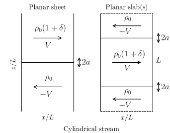
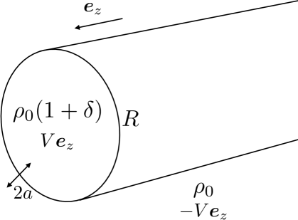
Figure 1: The planar sheet with one interface where the velocity changes sign (left), the planar slab (right) where the velocity changes sign twice and the cylindrical stream (bottom) where the velocity changes sign at $r=R$. We study the planar slab with two different boundary conditions in $z$: i) an infinite domain where disturbances are zero far from the shear interfaces and ii) a periodic domain which consists of two connected slabs where we identify the dashed boundaries.

2 The Kelvin-Helmholtz Instability

The simplest system in which the KHI can take place is the planar sheet, see Fig. 1. For this configuration, the flow velocity in the $x$-direction changes sign at $z=0$ with $\varv_{x}=-V$ for $z<0$ and $\varv_{x}=V$ for $z>0$. If we also allow for a difference in density with $\rho=\rho_{0}$ at the bottom and $\rho=\rho_{0}(1+\delta)$ at the top (where $\delta>-1$) and assume that disturbances are zero as $z\rightarrow\pm\infty$, then the dispersion relation for the KHI becomes (e.g., Chandrasekhar 1961)

$$\omega_{\pm}=\frac{\delta\pm i2\sqrt{1+\delta}}{2+\delta}kV\ ,$$ (1)

in the incompressible, inviscid hydrodynamic limit. Here $k$ is the wavenumber and the growth rate, $\sigma$, is given by the imaginary part of $\omega$, i.e., $\sigma\equiv-\mathrm{Im}(\omega)$. The discontinuous velocity profile is shown in the upper panel of Fig. 2 and the resulting growth rate with $\delta=0$ is shown in the lower panel of Fig. 2 with blue solid lines. Equation (1) and Fig. 2 show that the growth rate is proportional to the wavenumber such that doubling the grid resolution leads to a doubling of the growth rate of the fastest growing, resolved mode. This explains why a computer simulation will never converge with a discontinuous profile. In practice, numerical dissipation will damp wavenumbers close to the grid scale but the argument still holds because the scale for numerical dissipation depends on the grid resolution.

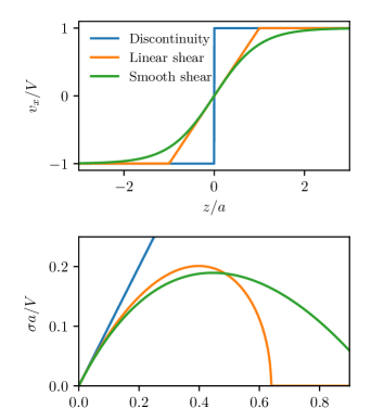
Figure 2: Introducing a smooth change in the direction of the velocity on a scale $\sim 2a$ prevent the KHI with wavelengths $\lambda\lesssim 2\pi a$ from growing. With sufficient spatial resolution, a smooth profile thus makes it possible to resolve the full spectrum of the linear instability in numerical simulations.

The growth rate given by Equation (1) depends only on $k$ because there are no other length scales in the problem. Introducing a smoothing length, $a$, makes the growth rate dependent on this scale. However, smooth profiles have, as previously mentioned, no simple expression for the growth rates. For a three-zone model, in which the velocity has a linear profile between $z=-a$ and $z=a$ (see the orange solid line the upper panel of Fig. 2), an analytic expression can however be obtained as (Drazin & Reid, 2004)

$$\omega^{2}=\frac{V^{2}}{4a^{2}}\left[(2ka-1)^{2}-e^{-4ka}\right]\ ,$$ (2)

where $2a$ is the scale on which the velocity changes sign. The growth rate found using Equation (2) is shown in the lower panel of Fig. 2 with an orange solid line. In contrast to the discontinuous profile, the growth rate does not grow without bound. Instead, wavenumbers with $ka\gtrsim 0.6$ are stable. These high wavenumbers are not subject to the KHI because they correspond to wavelengths that are smaller than the scale on which the velocity changes sign.

The velocity profile in the three-zone model is continuous but its first derivative is discontinuous. For numerical simulations, a velocity profile of the form $\varv_{x}(z)=V\tanh(z/a)$ where $a$ is the smoothing length (shown with a green solid line in the upper panel of Fig. 2), has the advantage that both, the velocity and its derivatives are continuous. Analytical progress is however difficult, and instead we must resort to solving Rayleigh’s equation numerically (Michalke, 1964). Here Rayleigh’s equation, an eigenvalue equation derived from the fluid equations in the incompressible limit, is given by (Rayleigh 1879, see e.g., Pringle & King 2007)

$$\left(\frac{\omega}{k}-\varv_{x}\right)\left(\frac{d^{2}\delta\varv_{z}}{dz^{2}}-k^{2}\delta\varv_{z}\right)+\frac{d^{2}\varv_{x}}{dz^{2}}\delta\varv_{z}=0\ ,$$ (3)

where $\delta\varv_{z}(z)$ is the perturbed velocity in the $z$-direction. We solve Equation (3) on $z\in[-\infty,\infty]$ by using psecas and assume that $\delta\varv_{z}$ goes to zero at $z\rightarrow\pm\infty$. The resulting growth rates, originally obtained by Michalke (1964), are shown with a green solid line in the lower panel of Fig. 2. The qualitative features are identical to the three-zone model, i.e., introducing a smoothing length gives a $k_{\mathrm{cut}}$ above which the KHI does not grow. Introducing a smoothing length thus allows numerical simulations of the linear regime to converge.

The above discussion considered an incompressible flow on the infinite $z$-domain. Numerical astrophysical simulations, and the systems that they model, are however compressible, and often limited in spatial extent. This motivates introducing the planar slab shown in Fig. 1. The planar slab we consider is an over-dense central region with density $\rho_{0}(1+\delta)$ moving to the right surrounded by regions with density $\rho_{0}$ moving to the left. The planar slab introduces an extra length scale to the problem, i.e., the width of the slab, $L$. For discontinuous density and velocity profiles, the dispersion relation for this setup is derived in Mandelker et al. (2016). The boundary conditions that the perturbations go to zero as $z\rightarrow\pm\infty$ was assumed and a very detailed analysis of the dispersion relation was performed. In particular, it was found that the effective growth rate diverges logarithmically (Mandelker et al., 2016), i.e., $\sigma\propto\ln(kL)$. This means that the slab with a discontinuous profile is a problematic initial condition for numerical simulations.

The planar slab also allows for periodic boundary conditions in the $z$-direction because the fluid parameters (the base state) are identical on each side of the slab. By employing periodic boundary conditions in the $z$-direction, the planar slab becomes two slabs that are connected to each other on both sides. It is difficult to imagine a physical system with these properties and the two connected periodic slabs differ both qualitatively and quantitatively from the slab on an infinite domain (see Section 5). Nevertheless, the double periodic setup is very useful for code testing purposes if a smooth profile is considered (Lecoanet et al., 2016). Periodic boundary conditions can be implemented with machine precision and code testing with periodic boundary conditions thus ensures that numerical artifacts from the boundaries do not influence the simulation. Additionally, periodic boundary conditions in the $z$-direction eliminate the otherwise inevitable errors that would be associated with truncating the infinite $z$-domain. We therefore develop the linear theory and perform simulations of the periodic slab with smooth initial conditions in Section 4. The linearized equations that we derive in the next section are however not dependent on this choice of boundary conditions.

Finally, we will also discuss the KHI as it arises in a cylindrical stream (see Fig. 1) where the stream has velocity $V$ ($-V$) inside (outside) a certain radius, $R$. This configuration can be applied to cold flows in galaxy formation and has been extensively studied in Mandelker et al. (2016). Mandelker et al. (2016) assumed a discontinuous profile for the velocity and density while we introduce a smoothing length in radius, $a$. We calculate the growth rates and compare our findings to the results obtained from the analytical dispersion relation of Mandelker et al. (2016) in Section 5.3.

3 Equations and Equilibria

We consider three different sets of equations, i.e., the equations of inviscid hydrodynamics (e.g., Batchelor 2000), the equations of ideal MHD (e.g., Freidberg 2014) and the equations of Braginskii-MHD (Braginskii, 1965; Schekochihin et al., 2005). Braginskii-MHD, an extension of ideal MHD in which anisotropic transport of heat and momentum is described by the coefficients $\chi_{\parallel}$ and $\nu_{\parallel}$, reduces to ideal MHD in the limit $\chi_{\parallel}=\nu_{\parallel}=0$. In addition, ideal MHD reduces to inviscid hydrodynamics by setting $\bm{B}=\bm{0}$ in the equations. We thus introduce the equations of Braginskii-MHD and consider its various limits. The mass continuity equation, momentum equations, induction equation and entropy equation are given in SI units by

$$\frac{\partial{\rho}}{\partial{t}} =-\bm{\nabla}\bm{\cdot}\left(\rho\bm{\varv}\right)\ ,$$ (4)

$$\rho\frac{d\bm{\varv}}{dt} =-\bm{\nabla}p-\bm{\nabla}\bm{\cdot}\mathbf{\Pi}-\bm{\nabla}\bm{\cdot}\left(\frac{B^{2}}{2\mu_{0}}\mathbf{1}-\frac{B^{2}}{\mu_{0}}\mbox{\boldmath{$b$}}\mbox{\boldmath{$b$}}\right)\ ,$$ (5)

$$\frac{\partial{\bm{B}}}{\partial{t}} =\bm{\nabla}\bm{\times}\left(\bm{\varv}\bm{\times}\bm{B}\right)\ ,$$ (6)

$$\frac{p}{\gamma-1}\frac{d\ln\left(p\rho^{-\gamma}\right)}{dt} =-\mathbf{\Pi}\bm{:}\bm{\nabla}\bm{\varv}-\bm{\nabla}\bm{\cdot}\bm{Q}\ ,$$ (7)

where $\bm{a}\bm{b}$ is the dyadic product of vectors $\bm{a}$ and $\bm{b}$, $\rho$ is the mass density, $\bm{\varv}$ is the mean fluid velocity, $p$ is thermal pressure, $\bm{B}$ is the magnetic field with local direction $b$, $\mu_{0}$ is the magnetic permeability and $\gamma=5/3$ is the adiabatic index.

In Equations (4) to (7), the extra terms that are included in Braginskii-MHD, compared to the equations of ideal MHD, are the anisotropic heat flux, $\bm{Q}$, and the anisotropic viscosity tensor, $\mathbf{\Pi}$. These terms are included in order to model a plasma which is magnetized and weakly collisional. The anisotropic heat flux is given by

$$\bm{Q}=-\chi_{\parallel}\mbox{\boldmath{$b$}}(\mbox{\boldmath{$b$}}\bm{\cdot}\bm{\nabla}T)\ ,$$ (8)

where $\chi_{\parallel}$ is the heat conductivity and the anisotropic viscosity tensor is given by

$$\mathbf{\Pi}=-\rho\nu_{\parallel}\left(3\mbox{\boldmath{$b$}}\mbox{\boldmath{$b$}}\bm{:}\bm{\nabla}\bm{\varv}-\bm{\nabla}\bm{\cdot}\bm{\varv}\right)\left(\mbox{\boldmath{$b$}}\mbox{\boldmath{$b$}}-\frac{\mathbf{1}}{3}\right)\ ,$$ (9)

where $\nu_{\parallel}$ is the viscosity coefficient. The anisotropic transport coefficients are assumed to be given by their Spitzer values (Spitzer, 1962; Braginskii, 1965), i.e., $\chi_{\parallel}=\chi_{\parallel,0}(T/T_{0})^{5/2}$ and $\nu_{\parallel}=\nu_{\parallel,0}\,\rho_{0}/\rho\,(T/T_{0})^{5/2}$, where $\chi_{\parallel,0}$ and $\nu_{\parallel,0}$ are reference values.

3.1 Linearized Equations

We consider an equilibrium magnetic field and velocity which is in the $x$-direction and have magnitudes that can vary along $z$, i.e., given by $\bm{B}=B(z)\bm{e}_{x}$ and $\bm{\varv}=\varv(z)\bm{e}_{x}$. We also allow the density, temperature and pressure to vary with $z$, i.e. $\rho(z)$, $T(z)$ and $p(z)$ with $p(z)=k_{\textup{B}}\rho(z)T(z)/\mu m_{\textup{H}}$ where $k_{\textup{B}}$ is Boltzmann’s constant, $m_{\textup{H}}$ is the proton mass and $\mu$ is the mean molecular weight. The only requirement on $B(z)$ and $p(z)$ is that equilibrium demands

$$\frac{d}{dz}\left(\frac{B^{2}}{2\mu_{0}}+p\right)=0\ .$$ (10)

We linearize Equations (4) to (7) in order to study the linear stability properties of a given equilibrium profile. We use a Fourier transform in the $x$-direction but retain the derivatives in the $z$-direction. A Fourier transform cannot be used in the $z$-direction because of the non-trivial $z$-dependence of the equilibrium. The perturbations have the form $f_{k}(z)\exp(ikx-i\omega t)$ where $f(z)$ is a $z$-dependent Fourier amplitude of a given variable. We assume that the solutions are constant along the $y$-direction. In effect, this corresponds to linearizing the equations with

$$\rho \rightarrow\rho(z)+\delta\rho(x,z)\ ,$$ (11)

$$T \rightarrow T(z)+\delta T(x,z)\ ,$$ (12)

$$\bm{\varv} \rightarrow\varv(z)\bm{e}_{x}+\delta\bm{\varv}(x,z)\ ,$$ (13)

$$\bm{B} \rightarrow B(z)\bm{e}_{x}+\delta\bm{B}(x,z)\ ,$$ (14)

and performing the Fourier transform in time and in the $x$-direction.

We introduce a vector potential $\bm{A}=A(z)\bm{e}_{y}$ such that the magnetic field is given by $\bm{B}=\bm{\nabla}\bm{\times}\bm{A}$. It follows that the perturbation to the magnetic field is given by $\delta\bm{B}=\bm{\nabla}\bm{\times}(\delta A\bm{e}_{y})$ such that

$$\delta B_{x} =-\frac{\partial{\delta A}}{\partial{z}}\ ,$$ (15)

$$\delta B_{z} =ik\delta A\ .$$ (16)

The advantage gained by introducing the vector potential is that the induction equation is reduced to a single equation (instead of two). We obtain a set of linearized equations given by the continuity equation,

$$-i\omega\frac{\delta\rho}{\rho} =-ik\left(\varv\frac{\delta\rho}{\rho}+\delta\varv_{x}\right)-\left(\frac{d\ln\rho}{dz}+\frac{\partial{}}{\partial{z}}\right)\delta\varv_{z}\ ,$$ (17)

the $x$-component of the momentum equation,

$$-i\omega\delta\varv_{x} =-ik\varv\delta\varv_{x}-\frac{\partial{\varv}}{\partial{z}}\delta\varv_{z}-ikc^{2}\left(\frac{\delta\rho}{\rho}+\frac{\delta T}{T}\right)+ik\varv_{a}^{2}\frac{d\ln B}{dz}\frac{\delta A}{B}$$

$$-\nu_{\parallel}\left(\frac{4}{3}k^{2}\delta\varv_{x}+2k^{2}\frac{\partial{\varv}}{\partial{z}}\frac{\delta A}{B}+\frac{2}{3}ik\frac{\partial{\delta\varv_{z}}}{\partial{z}}\right)\ ,$$ (18)

the $z$-component of the momentum equation,

$$-i\omega\delta\varv_{z} =-ik\varv\delta\varv_{z}-c^{2}\frac{\partial{}}{\partial{z}}\left(\frac{\delta\rho}{\rho}+\frac{\delta T}{T}\right)+c^{2}\frac{d\ln p}{dz}\left(\frac{\delta\rho}{\rho}-\frac{\delta T}{T}\right)$$

$$+\frac{\varv_{a}^{2}}{B}\left[\frac{\partial^{2}{}}{\partial{z}^{2}}+\frac{d\ln B}{dz}\frac{\partial{}}{\partial{z}}-k^{2}\right]\delta A$$

$$\>-\nu_{\parallel}\left(\frac{5}{2}\frac{d\ln T}{dz}+\frac{\partial{}}{\partial{z}}\right)\left(\frac{2}{3}ik\delta\varv_{x}+ik\frac{\partial{\varv}}{\partial{z}}\frac{\delta A}{B}-\frac{1}{3}\frac{\partial{\delta\varv_{z}}}{\partial{z}}\right)\ ,$$ (19)

an equation for the magnetic vector potential,

$$-i\omega\frac{\delta A}{B} =\delta\varv_{z}-ik\varv\frac{\delta A}{B}\ ,$$ (20)

and the entropy equation,

$$-i\omega\frac{\delta T}{T} =-ik\left(\varv\frac{\delta T}{T}+\frac{2}{3}\delta\varv_{x}\right)-\left(\frac{d\ln T}{dz}+\frac{2}{3}\frac{\partial{}}{\partial{z}}\right)\delta\varv_{z}$$

$$-\frac{2k^{2}\chi_{\parallel}T}{3p}\left(\frac{\delta T}{T}+\frac{d\ln T}{dz}\frac{\delta A}{B}\right)\ .$$ (21)

Here we have introduced the squared Alfvén speed

$$\varv_{a}^{2}=\frac{B^{2}}{\mu_{0}\rho}\ ,$$ (22)

and the squared isothermal sound speed

$$c^{2}=\frac{p}{\rho}\ ,$$ (23)

which define the plasma-$\beta$

$$\beta\equiv\frac{2c^{2}}{\varv_{a}^{2}}\ .$$ (24)

Equations (17) to (21) constitute an eigenvalue problem that we solve using the Python framework psecas which we describe in the next section.

3.2 psecas: A Python package for pseudo-spectral eigenvalue problems in (astrophysical) fluid dynamics

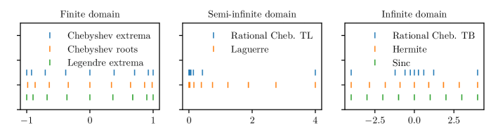
Figure 3: Illustration of eight of the nine grids implemented in psecas with $N=9$ grid points. The grids used for finite domains have the grid points closely packed at the boundaries (left panel) while the semi-infinite (middle panel) and infinite grids (right panel) have their grid points packed close to the origin. For the grids used for finite domains, the packing of grid points prevents high frequency oscillations close to the boundaries. For the (semi)-infinite grids, the placement of grid points helps with obtaining good spatial resolution at the region of interest while covering a large extent that mimics the (semi)-infinite domain. One exception is the Sinc grid which is equally spaced and which therefore requires many grid points to model the infinite domain. The last grid available in psecas is the periodic Fourier grid which has a uniform spacing (not shown). More details can be found in Table 1 and in Boyd (2000).

psecas is a newly developed Python package for using pseudo-spectral methods to semi-automatically generate and solve eigenvalue problems. The motivation for writing this package is to facilitate solving the complicated eigenvalue problems that often arise in (astrophysical) fluid dynamics. Examples of such eigenvalue problems (besides the ones studied in this paper) include the quasi-global theory of the heat-flux-driven buoyancy instability (Latter & Kunz, 2012), the heat-and-particle-flux driven buoyancy instability (Berlok & Pessah, 2016), the magnetorotational instability with the Hall effect (Hall-MRI, Béthune et al. 2016; Krapp et al. 2018), the thermal instability in galaxy clusters (Choudhury & Sharma, 2016) and the vertical shear instability (Umurhan et al., 2016).

psecas works by generating a matrix eigenvalue problem from a linearized set of equations by using the pseudo-spectral method to discretize the equations (see e.g., Fornberg 1996; Trefethen 2000; Boyd 2000). Users can enter their equations as strings which are then parsed by the program, allowing a close resemblance between code and the equations as they appear on paper. This reduces the risk of introducing errors when solving complicated linearized equations such as Equations (17) to (21).

The key ingredient in pseudo-spectral methods is the grid and the corresponding polynomials used to discretize the problem. psecas contains several options for solving problems on a periodic interval (e.g., $z\in[0,\,2\pi]$), a finite interval $z\in[0,\,L]$, a semi-infinite interval $z\in[0,\,\infty]$ or an infinite interval $z\in[-\infty,\,\infty]$. These are summarized in Fig. 3 and in Table 1. In astrophysical fluid dynamics, the grids on the semi-infinite domain will typically be used to represent the radial coordinate in spherical or cylindrical polar coordinates. The grids on the infinite domain are useful for e.g., representing the distance above the midplane in a galactic disk or accretion disk. In this paper we use the Fourier grid for the planar slab on a periodic domain, the rational Chebyshev TB grid for the planar slab on an infinite domain and the rational Chebyshev TL grid for the cylindrical stream. The finite grids are useful for studying e.g., plane-parallel atmospheres and can also be used for the KHI with reflective boundaries.

Given a set of $d$ linearized equations and a specified grid with $N$ grids points psecas automatically generates a (generalized) matrix eigenvalue problem of dimension $Nd\times Nd$. The matrix eigenvalue problem is solved using Scipy (Jones et al., 2017) which returns $N$ eigenvalues most of which will not be physical but numerical (Boyd, 2000). An important aspect of solving eigenvalue problems with pseudo-spectral methods is therefore ensuring that the computed eigenvalues have converged and are physical (Boyd 2000, definition 16). psecas has functionality for iteratively increasing the number of grid points until the obtained growth rates differ by less than a user-specified tolerance with respect to the previous iteration. For large $N$, which might be required for convergence, solving the full eigenvalue problem can be computationally intensive. For instability studies, one is however often only interested in the fastest growing eigenvalues. To take advantage of this, psecas contains functionality for only finding a single eigenvalue in the vicinity of a guess. This functionality is used for iteratively finding converged solutions, i.e., by using the result from a previous iteration as a guess for the next iteration at higher grid resolution. To further enable large parameter studies, psecas uses the message passing interface (MPI) to distribute calculations to several hundred processors (Dalcín et al., 2008).

A common task for instability studies is finding the maximal growth rate of the instability. psecas uses golden section search (Press et al. 2007, section 10.2) for finding the maximum of an instability with respect to a given parameter. This facilitates finding the maximally growing wavenumber to a specified precision, e.g., $10^{-8}$ for the calculations presented in Table 2.

3.3 Equilibria

We consider the periodic slabs (see Fig. 1) with an equilibrium velocity profile given by (Lecoanet et al., 2016)

$$\frac{\varv(z)}{V}=\tanh\left(\frac{z-z_{1}}{a}\right)-\tanh\left(\frac{z-z_{2}}{a}\right)-1\ ,$$ (25)

where $z_{1}=L/2$, $z_{2}=3L/2$ and $a=0.05L$ is a smoothing length. This profile is periodic on the domain $z=[0,2L]$ and changes direction at $z_{1}$ and $z_{2}$ where the KHI can be triggered. The magnitude of the velocity is set by the free parameter $V$. Following Lecoanet et al. (2016), we also allow for a density variation

$$\frac{\rho(z)}{\rho_{0}}=1+\frac{\delta}{2}\left[\tanh\left(\frac{z-z_{1}}{a}\right)-\tanh\left(\frac{z-z_{2}}{a}\right)\right]\ ,$$ (26)

with a magnitude set by the parameter $\delta$. With $\delta=0$ the background density is uniform. Equations (17) to (21) allow for general variations of pressure, $p(z)$, and magnitude of the magnetic field strength, $B(z)$, as long as Equation (10) is fulfilled. Here we consider the simplest configuration of this type, where both background pressure and magnetic field strength are constant. This yields the temperature variation

$$\frac{T(z)}{T_{0}}=\frac{\rho_{0}}{\rho(z)}\ ,$$ (27)

and an initial magnetic field which is completely specified by the plasma-$\beta$. Anisotropic transport does not affect the equilibrium, which has zero heat and momentum flux regardless of the values of $\chi_{\parallel}$ and $\nu_{\parallel}$ when the magnetic field is in the $x$-direction.

Table 1: The nine grids available in psecas.

Domain	Grid	Reference
Periodic
	Fourier	Trefethen (2000)
Finite
	Chebyshev extrema	Boyd (2000) F.8
	Chebyshev roots	Boyd (2000) F.9
	Legendre extrema	Boyd (2000) F.10
Semi-infinite
	Rational Chebyshev, TL	Boyd (1987b)
	Laguerre	DMSuite
Infinite
	Rational Chebyshev, TB	Boyd (1987a)
	Hermite grid	DMSuite
	Sinc grid	Boyd (2000) F.7

Table 2: Parameters for the four examples of the KHI. Listed are also the fastest growing wavenumbers and the corresponding growth rates.

Name	$\beta^{-1}$	$\delta$	$\nu_{\parallel}/(Lc_{0})$	$k_{\mathrm{max}}L$	$\sigma_{\mathrm{max}}L/c_{0}$
H	0	0	0	5.1540899	1.7827486
H$\delta$	0	1	0	3.5128319	1.4035133
M	$0.2$	0	0	5.5775520	1.4614214
M$\nu$	$10^{-3}$	0	0.01	4.5470431	1.7087545

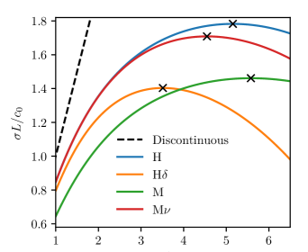
Figure 4: Growth rates as a function of wavenumber for the doubly periodic domain and the parameters listed in Table 2. Magnetic tension, viscosity and a density variation all inhibit the KHI and a density variation also turns the KHI into an overstability. A smooth transition on scale $a=0.05L$ inhibits growth at all scales visible in the plot and stabilizes the KHI at high wavenumbers. This is in contrast to the incompressible, analytic solution for a piece-wise constant velocity profile, which grows without bound (dashed black line, Equation 1 with $\delta=0$).

Using psecas, we discretize Equations (17) to (21) on a periodic Fourier grid in $z$ and approximate the differential operators using differentiation matrices. In this basis, periodic boundary conditions are automatically applied to the perturbations and the resulting matrix eigenvalue problem has dimension $5N\times 5N$ where $N$ is the number of grid points which is iteratively increased.

We consider four different cases which are chosen in order to test different parts of Athena. The four cases are hydrodynamics with a uniform density (H), hydrodynamics with a varying background density (H$\delta$), MHD with a strong magnetic field (M) and Braginskii-MHD with a weak magnetic field and anisotropic viscosity (M$\nu$). We set the flow velocity to be $V/c_{0}=1$ in all four cases and summarize their other parameters in Table 2. Here $c_{0}=\sqrt{p_{0}/\rho_{0}}$ is the isothermal sound speed at temperature $T_{0}$, which is related to the isothermal sound speed in the denser slab by $c_{s}=c_{0}/\sqrt{\delta+1}$.

The resulting growth rates are shown in Fig. 4 where we have defined $\sigma\equiv-\mathrm{Im}(\omega)$. All of the calculations with $\delta=0$ have $\mathrm{Re}(\omega)=0$, i.e., they are purely growing instabilities. Only the KHI with a density variation, $\delta\neq 0$, has $\mathrm{Re}(\omega)\neq 0$, and we find that $\mathrm{Re}(\omega)=\pm 0.5422067$ when $k=k_{\mathrm{max}}$. This corresponds to an oscillating or a traveling growing mode. The fastest growing mode for each set of physical parameters is indicated with black crosses in Fig. 4. The corresponding values of $k_{\mathrm{max}}$ and $\sigma_{\mathrm{max}}$ are given in Table 2. These values have been calculated within a tolerance of $10^{-8}$. It is clearly seen in Fig. 4 and Table 2 that the fastest growing instability is found when the background density is uniform (blue) and that the instability is inhibited when a density variation is introduced. This qualitatively agrees with the expectation from Equation (1), derived in the incompressible limit for the planar sheet (Chandrasekhar, 1961). The KHI with a uniform background is inhibited by Braginskii viscosity (Suzuki et al., 2013) and by magnetic tension (Chandrasekhar, 1961; Miura & Pritchett, 1982). We observe that Braginskii viscosity does not damp the long wavelengths as viscosity is ineffective on those scales for the chosen value of the viscosity parameter (magnetic tension is negligible for this calculation).

Besides the eigenvalues, psecas also returns the eigenvectors of the eigenvalue problem, i.e., numerical solutions for $\delta\rho/\rho$, $\delta T/T$, $\delta\varv_{x}$, $\delta\varv_{z}$ and $\delta A$. These can be used to construct the two-dimensional linear solutions of the initial value problem. We use the obtained two-dimensional linear solutions to initialize simulations with Athena in the following section.

4 Simulations of surface modes

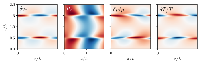
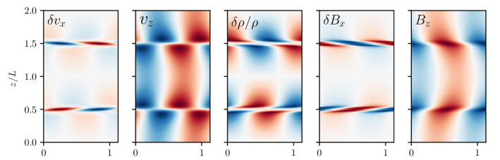
Figure 5: Deviations from the background functions, Equations (25) and (26), in two of the Athena simulations. The shear-interfaces are located at $z/L=1/2$ and $z/L=3/2$ giving rise to pronounced disturbances at those locations. All images are visually indistinguishable from the linear solution given by Equation (28). Upper row: Simulation of the KHI with a background density variation ($\delta=1$). The modes are exponentially growing while moving to the right at a constant speed. Lower row: Simulation of the KHI with a magnetic field $\bm{B}=B\bm{e}_{x}$ which inhibits the instability ($\beta=5$). The modes are purely growing.

We use the publicly available MHD code Athena to perform the tests (Gardiner & Stone, 2005, 2008; Stone et al., 2008). We consider a two-dimensional domain of size $L_{x}\times L_{z}$ where $L_{z}=2L$ and $L_{x}=2\pi/k_{\mathrm{max}}$ where $k_{\mathrm{max}}$ is the wavenumber for the fastest growing mode of the KHI for the given parameters (see Table 2). We set $L=\rho_{0}=p_{0}=1$ as code units and excite the instability by using the linear solutions found in the previous section. When initializing the simulations, each component of the perturbation, $\delta f(x,z,t)$ in real space, is related to its $z$-dependent Fourier component, $f_{k}(z)$, by

$$\delta f(x,z,t)=2A\,\mathrm{Re}\left[f_{k}(z)e^{-i\omega t+ikx}\right]\ ,$$ (28)

where $A=10^{-4}$ is the amplitude of the perturbation. The eigenmodes returned by psecas are given at the grid points illustrated in Figure 3 but can equivalently be expressed in terms of the corresponding basis functions, i.e.,

$$f_{k}(z)=\sum_{l}c_{l}P_{l}(z)\ ,$$ (29)

where $P_{l}(z)$ is a set of basis functions and $c_{l}$ are the corresponding coefficients (Boyd, 2000). For the Fourier grid considered here, Equation (29) is simply a Fourier series and $P_{l}(z)$ are complex exponentials. For the polynomial grids, $P_{l}(z)$ are the corresponding polynomials (e.g., Legendre polynomials for the Legendre grid). This means that psecas solutions can be evaluated at any location with spectral accuracy by using Equation (29) (Trefethen, 2000).

We evaluate all perturbed gas quantities (density, pressure and velocities) at the grid cell centers in Athena. For the MHD simulations the magnetic field requires special treatment. Here we evaluate the vector potential at cell faces instead of cell centers. The magnetic field is then initialized using finite differences. This ensures that the magnetic field has zero divergence to machine precision.

We perform the simulations on a grid with $N_{z}=256$ and $N_{x}=N_{z}L_{x}/L_{z}$ (rounding up to nearest integer). We use 3rd order reconstruction and Corner Transport Upwind (CTU, Colella 1990) with the Harten-Lax-van Leer with contact Riemann solver for the hydrodynamic simulations (HLLC, Toro 2013) and the Harten-Lax-van Leer with contact and Alfvén mode Riemann solver for the MHD simulations (HLLD, Miyoshi & Kusano 2005). We set the Courant number to 0.8 and evolve the simulations until $c_{0}t/L=10$.

In Fig. 5 we show snapshots from two of the simulations during the linear phase of the instability. In the upper row of Fig. 5 we show the difference of all four components of the solution with respect to the equilibrium at $c_{0}t/L=5$ for the simulation with a density variation (H$\delta$). At this point in time the perturbations have grown by a factor $\sim 10^{3}$ and the visual appearance is indistinguishable from the analytic solution evaluated using Equation (28). The mode is moving to the right at speed $\varv_{\mathrm{ph}}=\mathrm{Re}{(\omega)}/k$.

In the lower panel of Fig. 5, we show similar results for the MHD simulation with $\beta=5$ (here at $c_{0}t/L=3$ due to the larger growth rate). For this simulation we also present the $z$-component of the magnetic field and the perturbation to the $x$-component. This instability is purely growing and the spatial form of the perturbation is therefore constant in time during the linear phase of the instability, i.e., it is only the magnitude of the perturbation that changes.

A notable feature of the modes in Fig. 5 are the strong variations close to the shear layers located at $z_{1}$ and $z_{2}$. Away from the surfaces of the shear layers, the perturbations are much smaller. For that reason, these modes are called surface modes. At the flow velocity considered, i.e., $V/c_{0}=1$, the solutions found in Table 2 and Fig. 4 are all surface modes. This is in contrast to body mode disturbances which extent throughout the entire domain. We study the body modes that arise when the flow velocity is higher, $V/c_{0}=2.5$, in Section 5.

For code testing, inspection of the components of the perturbation shown in Fig. 5 can aid in diagnosing errors in the source code by visually identifying the component in which the error initially occurs. This type of visual inspection is much more difficult if the instability is not excited by an eigenmode. A visual inspection is of course not sufficient for rigorous code testing. In Fig. 6 we show the evolution of perturbations from the background equilibrium for all four simulations. As expected, we observe a nearly perfect exponential evolution of all quantities in all four cases. There is no initial transient and we can therefore estimate the growth rates for the simulations without ignoring the first part of the data. This is another advantage compared to simulations where the instability is seeded with random perturbations or a non-eigenmode analytic expression. We fit an exponential time evolution of the form $h(t)=a\exp(\sigma_{\mathrm{fit}}t)$ to the time interval $c_{0}t/L=0-2$ and calculate the relative error of the fitted growth rate as $|\sigma_{\mathrm{fit}}-\sigma|/\sigma$. We find agreement with the theoretical values listed in Table 2 with a relative error of between $3\cdot 10^{-3}$ and $5\cdot 10^{-3}$ depending on which of the quantities we fit. This error should decrease with numerical resolution and can be used for convergence testing. As an example, we consider hydrodynamic simulations of the H$\delta$ model with $\delta=1$ at four different resolutions, $N_{x}=64$, 128, 256 and 512 and show in the left panel of Fig. 7 that the relative error in the growth rate converges at second order.

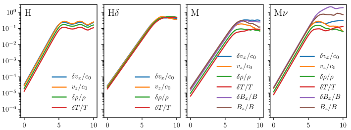
Figure 6: Exponential growth of deviations from the background equilibrium in the four simulations listed in Table 2. The exponential growth starts without an initial transient because the linear solution is used to excite the instability. The fitted growth rates agree with the theory to within $5\cdot 10^{-3}$ regardless of which component we use for the fit. Nonlinear effects, not captured by the linear theory, eventually cause the instability to saturate.

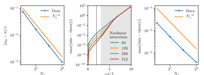
Figure 7: Convergence study of Athena simulations to psecas solutions for the H$\delta$ model. Left: Second order convergence of the fractional error in the fit of the growth rate. Middle: Maximum difference between linear solution for $\varv_{z}$ and simulations with increasing grid resolution, $N_{x}$, as a function of time. The gray area roughly indicates the region in which nonlinear effects are important. Data points from the linear regime (indicated with a black dashed line) are extracted and shown in the right panel. Right: Second order convergence of the maximum difference between the linear solution and simulations at $c_{0}t/L=2$.

We can also use the linear solution for convergence testing by directly measuring the difference between the Athena solution and the linear solution. We again consider simulations of the H$\delta$ model with $\delta=1$ at four different resolutions, $N_{x}=64$, 128, 256 and 512. For each simulation snapshot, we then calculate the maximum value of the absolute difference between the linear solution for $\varv_{z}(x,z,t)$ given by Equation (28) and the simulation snapshot. We show how the absolute maximum of this difference grows as a function of time in the middle panel of Fig. 7.

As Athena solves the full nonlinear equations of hydrodynamics, Equations (4) to (7), the difference grows without bound at late times. This is because the KHI in the Athena simulation saturates in the non-linear regime while the linear solution predicts continued exponential growth. The difference at large times is thus not due to errors in Athena but rather due to the neglect of higher order terms in Equations (17) to (21). At early times ($c_{0}t/L\lesssim 3$), however, where nonlinear terms are small, we do observe a decrease in the difference between Athena and the linear solution as the numerical resolution is increased. This difference is due to finite resolution in Athena and it converges at second order, see the right panel of Fig. 7.

5 High-Mach-number flows with body modes

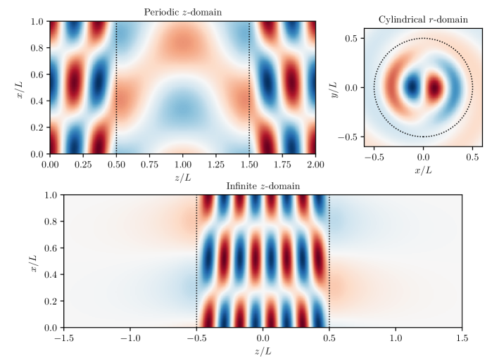
Figure 8: The KHI in three different setups. At high flow speeds $V/c_{0}=2.5$ an over-dense slab ($\rho=2\rho_{0}$) gives rise to pressure profiles that are not confined to the surfaces of the shear interfaces (indicated with black dotted lines) but rather extent throughout the interior of the slab. These are body modes (or reflective modes) which consist of soundwaves that are resonant inside the body of the slab. The periodic $z$-domain consists of two connected slabs with body modes inside both of them, and the pressure perturbation thus extends the entire domain. This is in contrast to the infinite $z$-domain and the cylindrical $r$-domain where the perturbations decay with distance from the surfaces of the slab. The calculations have been performed with psecas and a smoothing length $a=0.05L$. The Cartesian calculations show modes with $k=k_{x}=2\pi/L$ while the cylindrical calculation used $k=k_{z}=2\pi/L$ and azimuthal wavenumber $m=1$ (dipole).

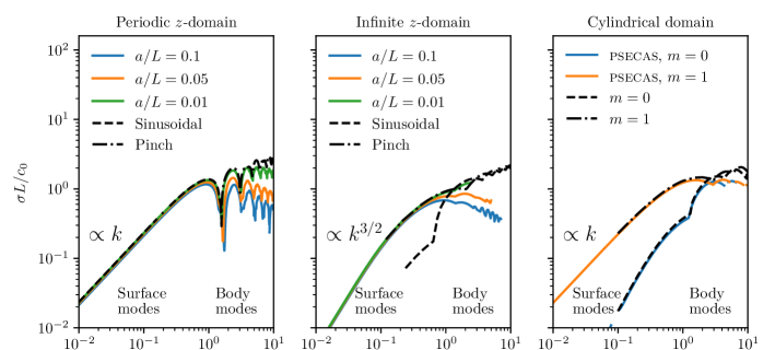
Figure 9: Dispersion plots for the KHI in the three different setups with $V/c_{0}=2.5$ and $\delta=1$. We compare results from the analytic dispersion relations derived for discontinuous density and velocity profiles with growth rates found using psecas and smooth profiles. Generally, the results coincide at low wavenumbers (long wavelengths) where the smoothing is insignificant. At high wave numbers the growth rates diverge for the discontinuous profiles but are diminished when the profiles are smooth. The low wavenumber solutions are surface modes while the high wavenumber solutions are body modes. Left and middle panel: we compare the growth rates for the periodic and the infinite $z$-domain. We observe that the scaling with $k$ differs at low wavenumbers with $\sigma\propto k$ for the periodic $z-$domain and $\sigma\propto k^{3/2}$ for the infinite domain. The growth rates at various smoothing lengths converge to the analytic theory as the smoothing length is decreased with a slower convergence at high $k$. Right panel: the growth rates for azimuthal modes with $m=0$ and $m=1$ in cylindrical geometry. The psecas solutions have little smoothing ($a=0.01L$) and consequently agree with the analytic dispersion relation except at high $k$.

For the planar sheet, i.e., a single interface at which the velocity changes direction (see left panel of Fig. 1), the KHI is stabilized when the flow velocity is sufficiently high (Landau, 1944; Mandelker et al., 2016). This occurs when the flow velocity (see eq. 22 in Mandelker et al. 2016)

$$\frac{V}{c_{0}}>\frac{1}{2}\sqrt{\frac{\gamma}{1+\delta}}\left[1+(1+\delta)^{-1/3}\right]^{3/2}\approx 1.1\ ,$$ (32)

for $\delta=1$ and $\gamma=5/3$.

For the planar slab (see the right panel of Fig. 1) discussed in Section 4 a different type of KHI can however arise at high flow velocities. These are interchangeably called reflective modes (Payne & Cohn, 1985; Hardee & Norman, 1988) or body modes (Mandelker et al., 2016). Reflective modes because the instability consists of soundwaves that are reflected between the interfaces of the slab and body modes because it highlights that the KHI disturbances occur throughout the slab and not just at its surfaces. In this section we analyze the body modes in the periodic Cartesian domain, the Cartesian infinite domain and in cylindrical geometry. Examples of the pressure perturbation for body modes with $V/c_{0}=2.5$ and $\delta=1$ in the various setups are shown in Fig. 8. In these figures the density and the direction of the velocity changes at the interfaces indicated with dotted black lines. This change is smooth on a scale $a/L=0.05$ and the solutions have been obtained with psecas.

In the following subsections we provide details for these calculations and consider solutions where we decrease the smoothing parameter, $a$, thus imitating a discontinuous profile. These solutions are compared with the analytic theory for the discontinuous profiles for the slab in an infinite Cartesian domain and the cylindrical slab presented in (Mandelker et al., 2016). For the periodic Cartesian domain used in Section 4 and by Lecoanet et al. (2016), we derive the analytic theory for discontinuous profiles by following the procedure outlined in Mandelker et al. (2016) while taking the different boundary conditions into account. We obtain a dispersion relation, which yields growth rates that differ from those found on the infinite domain.

A common element for the analysis in the following sections is the generalized wavenumber

$$q=k\sqrt{1-\frac{(\omega-k\varv)^{2}}{k^{2}\gamma c^{2}}}\ ,$$ (33)

where $k=k_{x}$ in Cartesian geometry and $k=k_{z}$ in cylindrical geometry. The generalized wave number depends on velocity and density and has different values in the slab (or stream) and in the background. We refer to the background with 0 subscripts, and to the slab with a subscript $s$, e.g., $q_{0}$ and $q_{s}$.

5.1 Planar shear on a Cartesian, periodic domain

We consider the planar slab used for the simulation H$\delta$ in Section 4, i.e., $\delta=1$ and an equilibrium given by Equations (25) and (26) on a domain which is periodic in both $x$ and $z$. In order to study body modes, we increase the flow speed to $V/c_{0}=2.5$ such that Equation (32) is fulfilled and calculate the linear solution for $k=2\pi/L$. The resulting pressure perturbation is shown in the top left panel of Fig. 8. In this figure the equilibrium velocity and density change smoothly at $z/L=0.5$ and $z/L=1.5$. The pressure perturbation resulting from the KHI is not confined to these surfaces but instead extends throughout the domain. The perturbations are thus present both in the central slab (with $1/2<z/L<3/2$) and in the slab which, due to the periodicity in the $z$-direction, is the union of the regions with $z/L<1/2$ and $z/L>3/2$. The pressure perturbation is highest in the latter region where the density is lower. This phenomenon is also seen for KHI perturbations of surface modes which penetrate deeper into the fluid with lower density (see e.g., Fig. 2 in Mandelker et al. 2016).

The structure of the mode is qualitatively different from the corresponding mode on the infinite domain (see Fig. 8). Here the pressure perturbation is confined to the central slab and decays abruptly outside of it. The key difference is that the periodic domain consists of two slabs that are connected with each other on both sides. We have seen in Section 4 that this setup can be very useful for code testing purposes. Whether this setup can be used to model the KHI in a real physical application is however not obvious. In the following we discuss the difference between the two setups by calculating growth rates for the KHI in the two different setups using both analytic theory for discontinuous profiles and psecas for smooth profiles.

We begin by deriving the analytic dispersion relation for the two connected slabs on a periodic domain when the profiles are discontinuous. The derivation closely follows the analysis of the slab on the infinite domain presented in Mandelker et al. (2016). We consider three domains where domain 1 has $z>L/2$, domain 2 has $|z|<L/2$ and domain 3 has $z<-L/2$. By combining Equation (17) and Equation (21) we obtain an equation for the pressure

$$-i\left(\omega-k\varv\right)\frac{\delta p}{p}=-ik\gamma\delta\varv_{x}-\gamma\frac{\partial{\delta\varv_{z}}}{\partial{z}}\ ,$$ (34)

where $\delta\varv_{x}$ and $\delta\varv_{z}$ are given by

$$-i\left(\omega-k\varv\right)\delta\varv_{x} =-\frac{\partial{\varv}}{\partial{z}}\delta\varv_{z}-ik\frac{\delta p}{\rho}\ ,$$ (35)

and

$$-i\left(\omega-k\varv\right)\delta\varv_{z} =-\frac{1}{\rho}\frac{\partial{\delta p}}{\partial{z}}\ .$$ (36)

These are simply simplified forms of Equations (18) and (19) where the background magnetic field, the pressure gradient etc. have been set to zero. We combine Equations (34) to (36) and find a second order, ordinary differential equation (ODE) for the perturbed pressure

$$\frac{\partial^{2}{\delta p}}{\partial{z}^{2}}+\left(\frac{2k}{\omega-k\varv}\frac{\partial{\varv}}{\partial{z}}-\frac{1}{\rho}\frac{\partial{\rho}}{\partial{z}}\right)\frac{\partial{\delta p}}{\partial{z}}-q^{2}\delta p=0\ ,$$ (37)

which we solve analytically for piece-wise constant velocity and density profiles. Assuming discontinuous initial conditions, inside each of the three domains the density and velocity is constant and the terms in Equation (37) which are proportional to $\partial\delta p/\partial z$ are thus zero. The solution of Equation (37) is therefore simply $\delta p(z)/p=ae^{-qz}+be^{qz}$ where $q$ is given by Equation (33). The constants $a$ and $b$ are deduced by requiring that i) the solution is continuous across the domain interfaces at $z=\pm L/2$ and the interface at $z=\pm L$ and ii) the fluid displacement, $h$, is continuous across the interfaces. The latter requirement is known as the Landau condition (see e.g., Mandelker et al. 2016).

In order to derive the Landau condition, we consider the linearized equation for the interface displacement, $h$,

$$\frac{dh}{dt}=\delta\varv_{z}=-i(\omega-k\varv)h$$ (38)

which combined with the equation for $\delta\varv_{z}$ yields

$$h=-\frac{1}{\rho(\omega-k\varv)^{2}}\frac{\partial{\delta p}}{\partial{z}}$$ (39)

Applying the Landau condition at $z=\pm L$ as well as continuity of the solution, we find that the pressure profile is given by

$$\delta p(z)/p =A\,\mathcal{S}(-q_{0}[z-L]),\hskip 40.0pt z > L/2,$$ (40)

$$\delta p(z)/p =A\,\frac{\mathcal{S}(q_{0}L/2)}{\mathcal{S}(q_{s}L/2)}\mathcal{S}(q_{s}z), |z| < L/2,$$ (41)

$$\delta p(z)/p =A\,\mathcal{S}(-q_{0}[z+L]), z <- L/2,$$ (42)

where $\mathcal{S}(z)=\cosh(z)$ for symmetric pinch modes, $\mathcal{S}(z)=\sinh(z)$ for antisymmetric sinusoidal modes and $A$ is an overall amplitude. An illustration of the difference between sinusoidal and pinch modes can be found in Fig. 3 in Mandelker et al. 2016.

Applying the Landau condition at either $z=-L/2$ or $z=L/2$ then yields the dispersion relation for the two connected slabs in a periodic domain, given by

$$\left(\frac{\omega-k\varv_{s}}{\omega-k\varv_{0}}\right)^{2}=-\frac{\rho_{0}}{\rho_{s}}\frac{q_{s}}{q_{0}}\frac{\mathcal{T}(q_{s}L/2)}{\mathcal{T}(q_{0}L/2)}\ .$$ (43)

with $\mathcal{T}(z)=\tanh(z)$ for the pinch modes and $\mathcal{T}(z)=1/\tanh(z)$ for the sinusoidal modes.

We have found the maximum growth rate as a function of wavenumber by numerically solving Equation (43) for both pinch and sinusoidal modes. The results, presented in the left panel of Fig. 9 (black lines), show that the growth rate is highest for the sinusoidal modes at low wavenumbers and for the pinch modes at high wavenumbers.

Equation (43) can be solved analytically for $\omega$ in the incompressible limit, where $q_{0}=q_{s}=k$ and the terms with $\mathcal{T}$ cancel. The analytical result thus obtained is given by Equation (1), which was originally derived for the incompressible, planar sheet. The long wavelength $\sigma\propto k$ scaling of the growth rate is also found for the $m=0$ solution for the cylinder (Mandelker et al. 2016 and our Section 5.3) but the slab on the infinite domain has $\sigma\propto k^{3/2}$ (Mandelker et al., 2016). The chosen geometry can thus qualitatively change the pressure profile and the scaling of the growth rates with wavenumber.

We can also calculate the maximal growth rate as function of wavenumber using psecas. The result of such calculations with various smoothing lengths, $a$, are shown in the left panel of Fig. 9. At long wavelengths (small $k$), the psecas results and the sinusoidal mode solution of Equation (43) coincide with the incompressible limit of Equation (43), i.e., Equation (1). At short wavelengths where the solutions are body modes, smoothing of the profiles creates a difference between the solutions obtained with psecas and solutions to Equation (43). When the smoothing length is decreased and the smooth profile tends towards the discontinuous limit, this difference is reduced. Furthermore, the locations of peaks in the growth rate, are only weakly modified by the value of the smoothing coefficient. The underlying reason is that the peak locations are determined by a resonance condition which depends on the width of the slab (Payne & Cohn, 1985; Hardee & Norman, 1988; Mandelker et al., 2016).

For computer simulations of body modes, the smooth profiles have the attractive property that the growth rates at short wavelengths are inhibited. We consider a simulation of the fastest growing body mode when $a=0.05L$ in Fig. 10. We show the exponential growth of perturbations in the left panel of Fig. 10 and the fitted growth rate in the middle panel of Fig. 10. We find that the growth rate obtained from the simulation has a relative error of almost 2 %, significantly higher than the error found at lower flow velocities (i.e. the H$\delta$ simulation had $V/c_{0}=1$ compared to $V/c_{0}=2.5$ used for the body mode simulation). The maximum growth rate occurs at $kL=2.3629555$ where $\omega L/c_{0}=0.949814+1.440521i$.

5.2 Planar shear on Cartesian, infinite domain

We consider a slab located at $|z|<L/2$ on an infinite domain with $z\in[-\infty,\infty]$. We can study this setup with psecas by using the rational Chebyshev TB grid which models the infinite domain (Boyd, 1987a). A smooth velocity and density profile is described by Equations (25) and (26) with $z_{1}=-L/2$ and $z_{2}=L/2$. The resulting perturbed pressure profile for a body mode with $k=2\pi/L$ and $a/L=0.05$ is shown in Fig. 8. The body mode consists of sound waves inside the slab with perturbations that decay outside of it. Here, the pressure perturbation differs qualitatively from the corresponding perturbation on the periodic $z$-domain.

For a discontinuous profile, Mandelker et al. (2016) solved Equation (37) and applied the boundary conditions that the pressure perturbation goes to zero at $z\rightarrow\pm\infty$. By applying the Landau condition at either $z=-L/2$ or $z=L/2$, this yields the dispersion relation (Mandelker et al., 2016)

$$\left(\frac{\omega-k\varv_{s}}{\omega-k\varv_{0}}\right)^{2}=-\frac{\rho_{0}}{\rho_{s}}\frac{q_{s}}{q_{0}}\mathcal{T}(q_{s}L/2)\ .$$ (44)

with $\mathcal{T}(z)=\tanh(z)$ for the pinch modes and $\mathcal{T}(z)=1/\tanh(z)$ for the sinusoidal modes. A detailed analysis of this dispersion relation is presented in Mandelker et al. (2016), in the following we numerically solve Equation (44) in order to compare with solutions obtained with psecas and a smooth profile. This comparison is shown in the middle panel of Fig. 9 using three different smoothing lengths ($a/L=0.1$, $0.05$, and $0.01$).

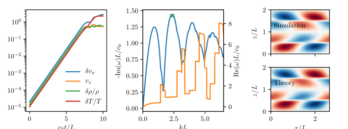
Figure 10: Simulation with $V/c_{0}=2.5$ and $\delta=1$. At these parameters, the fastest growing mode is a body mode, i.e., the mode structure extends far beyound the shear surfaces. Left: Evolution of perturbation amplitude in the Athena simulation. Middle: Growth rate (blue line) and real frequency (orange line) as a function of wavenumber with the growth rate from the Athena simulation indicated with a green cross. Right: The pressure perturbation in the simulation and evaluated using Equation (28) at $c_{0}t/L=5$.

At long wavelengths (where the solutions are surface modes), the psecas results and the pinch mode solution of Equation (44) both coincide with the incompressible limit of Equation (44) derived in Mandelker et al. (2018). At high wavelengths where the solutions are body modes, the smooth profile psecas solutions and the solutions to Equation (44) differ. This is again because a smooth profile lowers the growth rates. As for the periodic slab, this difference is reduced as the smoothing length is decreased towards the discontinuous limit.

Equation (44) has effective growth rates that diverge as $\sigma\propto\ln(kL)$ which makes convergence of simulations for the slab on the infinite domain unattainable with a discontinuous profile (Mandelker et al., 2016). For a sufficiently smooth profile, this divergence of the growth rate is removed and the growth rate is suppressed at high wave numbers.

5.3 Cylindrical KHI

We are interested in understanding the stability properties of a cylindrical stream of gas which moves at velocity $V$ through an ambient medium moving in the opposite direction with speed $-V$. Due to Galilean invariance of the equations this is equivalent to a stream of gas moving at $2V$ through a stationary medium. The setup is illustrated in Fig. 1. The stability properties of this system are important for understanding whether cold streams of gas can feed galaxies at high redshift or whether they are interrupted and heated by the KHI before reaching the galaxies (Mandelker et al., 2016; Padnos et al., 2018; Mandelker et al., 2018). We consider a cylindrical stream with diameter $L$ (radius $R=L/2$) and define a standard cylindrical coordinate system with unit vectors $\bm{e}_{r}$, $\bm{e}_{\phi}$ and $\bm{e}_{z}$. We take the background to only depend on the radial coordinate, $r$, with $\rho(r)$ and the velocity directed along $\bm{e}_{z}$, i.e., $\bm{\varv}=\varv(r)\bm{e}_{z}$.

We assume perturbations from this equilibrium of the form

$$f_{k,\,m}(r)e^{-i\omega t+im\phi+ikz},$$ (45)

which results in linearized hydrodynamical equations given by

$$-i\omega\delta\varv_{r} =-ik\varv\delta\varv_{r}-c^{2}\frac{\partial{}}{\partial{r}}\frac{\delta p}{p}\ ,$$ (46)

$$-i\omega\delta\varv_{\phi} =-ik\varv\delta\varv_{\phi}-im\frac{c^{2}}{r}\frac{\delta p}{p}\ ,$$ (47)

$$-i\omega\delta\varv_{z} =-ik\varv\delta\varv_{z}-\frac{\partial{\varv}}{\partial{r}}\delta\varv_{r}-ikc^{2}\frac{\delta p}{p}\ ,$$ (48)

and

$$-i\omega\frac{\delta p}{p} =-ik\varv\frac{\delta p}{p}-\gamma\frac{\partial{\delta\varv_{r}}}{\partial{r}}-\gamma\frac{\delta\varv_{r}}{r}-\gamma\frac{im}{r}\delta\varv_{\phi}-\gamma ik\delta\varv_{z}$$ (49)

in cylindrical coordinates. For the calculations with psecas, we take the background to be

$$\varv(r) =V\tanh\left(\frac{r-R}{a}\right)\ ,$$ (50)

$$\rho(r) =\rho_{0}+\rho_{0}\frac{\delta}{2}\left[1-\tanh\left(\frac{r-R}{a}\right)\right]\ ,$$ (51)

where $a$ is the smoothing parameter. In the limit $a\rightarrow 0$ this corresponds to a discontinuous profile with density $\rho_{0}(1+\delta)$ and velocity $V$ inside the stream and $(\rho,\varv)=(\rho_{0},-V)$ outside the stream.

Equations (46) to (49) are defined on $r\in[0,\infty]$ with a coordinate singularity at $r=0$. We use the rational Chebyshev TL polynomials to discretize the problem on this semi-infinite domain (Boyd, 1987b). Due to the coordinate singularity, this polynomial basis automatically applies boundary conditions that ensures that the perturbations are finite when $r\rightarrow 0$ and $r\rightarrow\infty$ (so-called behavioral boundary conditions, see Boyd 1987b, 2000). We take $k_{z}=2\pi/L$ and $m=1$ and calculate the resulting perturbed pressure profile which we show in Fig. 8. This mode is a body mode with a pressure perturbation that extends throughout the interior of the cylindrical stream.

We are again interested in comparing results from psecas using smooth profiles with analytic theory for discontinuous profiles. As for the Cartesian setup, the linearized equations, i.e., Equations (46) to (49), can be combined to obtain an ODE for the pressure perturbation (Mandelker et al., 2016)

$$\frac{\partial^{2}{\delta p}}{\partial{r}^{2}}+\left(\frac{2k}{\omega-k\varv}\frac{\partial{\varv}}{\partial{r}}-\frac{1}{\rho}\frac{\partial{\rho}}{\partial{r}}\right)\frac{\partial{\delta p}}{\partial{r}}-\left(q^{2}+\frac{m^{2}}{r^{2}}\right)\delta p=0\ .$$ (52)

Away from the interface where the terms proportional to $\partial\delta p/\partial r$ are zero, Equation (52) can be written as a modified Bessel equation. The solutions are therefore $\delta p/p=a\mathcal{I}_{m}(qr)+b\mathcal{K}_{m}(qr)$ where $\mathcal{I}_{m}$ ($\mathcal{K}_{m}$) is the modified Bessel function of the first (second) kind. Since the $\mathcal{I}_{m}\rightarrow\infty$ ($\mathcal{K}_{m}\rightarrow\infty$) as $r\rightarrow\infty$ ($r\rightarrow 0$) the solution has $b=0$ ($a=0$) inside (outside) the cylinder (Mandelker et al., 2016). Applying the Landau condition at $r=R$ yields the dispersion relation (Mandelker et al., 2016)

$$\left(\frac{\omega-k\varv_{s}}{\omega-k\varv_{0}}\right)^{2}=\frac{\rho_{0}}{\rho_{s}}\frac{q_{s}}{q_{0}}\frac{\mathcal{I}^{\prime}_{m}(q_{0}R)}{\mathcal{I}_{m}(q_{0}R)}\frac{\mathcal{K}_{m}(q_{s}R)}{\mathcal{K}^{\prime}_{m}(q_{s}R)}\ ,$$ (53)

which was derived and analyzed in detail by Mandelker et al. (2016).

The comparison between solutions of Equation (53) for the azimuthal wavenumbers $m=0$ and $m=1$ with the solutions obtained with psecas with a very short smoothing length ($a=0.01L$) are presented in Fig. 9. At long wavelengths, all solutions agree with the scalings derived in Mandelker et al. (2016).

6 Discussion

6.1 Code testing and verification

Tests of software used for modeling physical systems are generally classified as either verification or validation (see Oberkampf & Trucano 2002 for a review). In brief, code verification consists of ensuring that the code accurately solves the mathematical model (i.e., Equations (4) to (7) in our case) while validation assesses to which degree simulations agree with physical reality. In engineering, validation is achieved by comparing simulations with dedicated validation experiments (Oberkampf & Trucano, 2002). In computational astrophysics, validation is unfortunately very rarely possible using experiments and is instead assessed by comparing simulations to observations. Verification can be considered a preliminary of validation, and is therefore essential for astrophysical codes. Verification is normally done by comparing computer simulations with known analytical solutions or highly accurate numerical solutions. Analytical solutions to the nonlinear fluid equations have only been obtained in a very limited number of cases and many verification tests therefore compare simulations with analytical solutions of the linearized fluid equations.

Even finding an analytic solution to the set of linearized equations can however be problematic in some cases, e.g., when there is a non-trivial variation of the background equilibrium. This is the case for the KHI where analytical solutions have not been found for the smooth initial conditions that are required for convergence of simulations (Robertson et al., 2010; McNally et al., 2012; Lecoanet et al., 2016). The lack of an analytical reference solution for the KHI motivated the studies of McNally et al. (2012) and Lecoanet et al. (2016) who obtained accurate, numerical reference solutions in 2D by performing high resolution simulations of the KHI. Obtaining such reference simulations is very computationally intensive because high resolution is required in the two spatial dimensions and time. The reference solutions were made public by McNally et al. (2012) and Lecoanet et al. (2016) and are indispensable for verification of the nonlinear stage of the KHI during which vortex rolls form and secondary instabilities take place.

A linear reference solution would however be sufficient for verification of the linear regime. While such a linear reference solution has not been found analytically for the KHI with smooth initial conditions, it is possible to obtain an extremely accurate numerical solution using pseudo-spectral methods. In fact, the numerical linear solution can be found by discretization of only the direction perpendicular to the background flow while the direction parallel to the flow and the time evolution is treated analytically. The pseudo-spectral solution of the linearized equations therefore retains some of the useful properties of analytical solutions, i.e., that they can be evaluated to very high precision and that solutions with different physical parameters can be obtained rather quickly. For instabilities, the pseudo-spectral linear theory also makes it possible to determine the growth rate as a function of wavelength and the structure of the fastest growing mode. This knowledge provides important physical insight and can furthermore aid in designing nonlinear simulations. In particular, the growth rate versus wavelength determines what size the computational domain should be in order to resolve the full spectrum of the instability (e.g. Shalaby et al. 2017).

Using the MHD code Athena, we give an example of how pseudo-spectral linear theory can be used for inexpensive code verification of problems where analytic solutions are not available. We present simulations of the KHI with the smooth initial conditions used for convergence studies in Lecoanet et al. (2016) and additionally treat the MHD and Braginskii-MHD versions of the instability. We consider simulations of four different versions of the KHI (with parameters listed in Table 2) in which we seed the instability with the linear solution for the fastest growing eigenmode. We find excellent agreement between linear theory and simulations during the linear stage of the instability and this agreement is measured both in terms of the eigenmode structure and the growth rate. We also perform a convergence study and show that the relative error in both the eigenmode and the growth rate converge at second order. Importantly, we make material available online which can be used by readers to initialize the KHI with the linear solution. Alternatively, Table 2 can be used to confirm that the KHI in tests initialized with random perturbations grow at the maximum growth rate.

The Athena simulations presented in this paper were performed without MPI and still ran in less than a core hour in total. For comparison, the most expensive simulations presented in Lecoanet et al. (2016) took roughly $10^{6}$ core hours. In terms of computing time, it is therefore economical to do a convergence study of the linear regime before proceeding with a nonlinear convergence study. The linear tests presented in this paper can thus be useful for frequent, computationally inexpensive regression-tests of a code and two of the tests (H$\delta$ and M) have in fact already been included in the test suite of Arepo (Springel, 2010; Pakmor et al., 2011; Pakmor & Springel, 2013; Pakmor et al., 2016). Furthermore, one of the tests (M$\nu$) has proven very useful during the implementation of Braginskii viscosity in Arepo (Berlok et al., in prep.).

6.2 Astrophysical implications

6.2.1 Cold fronts in galaxy clusters

Sloshing cold fronts can arise when a cool-core galaxy cluster is subject to a minor merger. This leads to a disturbance in the ICM which exhibits a sloshing motion in the perturbed gravitational potential with a resulting cold front (see Markevitch & Vikhlinin 2007; ZuHone & Roediger 2016 for reviews). Cold fronts are cold and dense on one side and hot and dilute on the other side with a tangential velocity difference across the interface and should therefore be highly susceptible to the KHI. Observationally however, the KHI is not as abundantly observed as one would expect by applying, e.g., Equation (1) to observed values for densities and velocities. Possible explanations for this observational evidence for the suppression of the KHI include suppression by magnetic field tension (e.g. Vikhlinin et al. 2001; Dursi & Pfrommer 2008), viscosity (e.g. Roediger et al. 2013), Braginskii viscosity (e.g. Suzuki et al. 2013; Zuhone et al. 2015) or a finite width of the cold front (Churazov & Inogamov, 2004).

Most of these effects, except for isotropic viscosity, are captured by the linear theory derived in Section 3. We show in Figure 4 how Braginskii viscosity, magnetic fields, a smooth transition in the velocity profile and a density contrast all act to suppress the KHI. In the future, we intend to use Equations (17) to (21) and psecas to perform a detailed analysis of the stability properties of cold fronts, taking into account variations in magnetic field strength (due to magnetic draping), velocity, density and temperature across the cold front and using observationally inferred parameters (Berlok and Pfrommer, in prep.).

6.2.2 Cold streams feeding high redshift galaxies

Massive galaxies at redshifts $z=1-4$, with baryon mass $\sim 10^{11}M_{\odot}$ and dark matter halo virial mass $\sim 10^{12}M_{\odot}$, have star formation rates which are incompatible with the slow cooling rate of the virialized gas residing in the halo. Such massive galaxies are however located at nodes of the cosmic web, and the observed star formation rate ($\sim 100\,M_{\odot}$ yr^-1) is similar to the gas accretion found to occur along filaments in cosmological simulations. In contrast to the low density, $10^{6}$ K-virialized gas in the halo, the high density in the filaments allows the gas to efficiently cool to $10^{4}$ K before reaching the massive galaxy. A possible explanation for the observed star formation rate is thus that several cold, dense streams are able to penetrate through the hot, dilute gas and reach the central galaxy without being disrupted.

One potential disruption mechanism is the KHI, and a detailed understanding of the KHI is therefore important for understanding whether and how cold streams of gas can feed galaxies at high redshift (Mandelker et al., 2018). Cosmological simulations do not yet have the required spatial resolution to assess whether the KHI is present in cold streams and thus cannot be used for directly answering this question. As an alternative, Mandelker et al. (2016); Padnos et al. (2018); Mandelker et al. (2018) performed a very detailed study of the KHI using both analytical theory and simulations. Our results presented in Section 5, agree with growth rates calculated in Mandelker et al. (2016) for supersonic body modes in both planar slab and cylindrical geometry (see Figure 1 and 8). Additionally, we are able to calculate the suppression of short wavelength modes when there is a smooth transition in the velocity profile between the cold stream and the ambient medium. By assuming a smoothing length, $a$, we are able to calculate the maximal growth rate of body modes. This is in contrast to the analytic theory where the maximal growth rate diverges with wavenumber (Mandelker et al., 2016). Hence, our framework is able to account for more realistic density and velocity profiles when estimating how quickly cold streams will be disrupted by the KHI.

7 Conclusions

Smooth initial conditions are known to be a necessity for the convergence of computer simulations of the KHI, even for the linear stage (Robertson et al., 2010; McNally et al., 2012). Analytic predictions for the evolution of a simulation with such smooth initial conditions do however not exist, neither for the linear nor for the nonlinear regime of the instability. In lieu of analytic results, Lecoanet et al. (2016) has provided converged numerical results for the nonlinear regime of the hydrodynamic KHI as it occurs in a doubly periodic domain. Their simulations included explicit viscosity, heat conductivity and diffusion of a passive scalar and required very high grid resolution for convergence. As a supplement to convergence studies of the nonlinear regime, code tests of the linear stage are often used because they are computationally cheaper. Tests limited to the linear regime make it feasible to perform isolated testing of various physics modules and to explore a large parameter space. Such computer simulations are often compared with analytic results for discontinuous initial conditions because the analytical linear theory does not exist for smooth profiles. Quantitative comparisons between linear theory and simulations however require that the linear theory is derived with the same assumptions as the simulations. This includes boundary conditions, equation of state and (smoothness of) initial conditions.

With this problem in mind, we have derived the linear theory for the KHI with smooth initial conditions in both Cartesian and cylindrical geometry (illustrated in Fig. 1). The linear theory in Cartesian geometry combines and extends some of the results of previous work on the compressible hydrodynamic KHI (Blumen, 1970), the MHD version of the KHI (Miura & Pritchett, 1982) and the KHI with Braginskii viscosity (Suzuki et al., 2013).

The simulations discussed in Section 4 (and the ones presented in Lecoanet et al. 2016) used a subsonic flow velocity where the KHI appears as surface modes, i.e., the disturbances to the flow are localized at the shear interfaces. At supersonic flow velocities, the KHI can manifest itself as body modes that have disturbances with much larger extent (Payne & Cohn, 1985; Hardee & Norman, 1988; Mandelker et al., 2016). Specializing to the equations of inviscid hydrodynamics, we analyze body modes in both Cartesian and cylindrical geometries. We compare our results found with initial conditions that are smooth on a scale, $2a$, with analytic theory derived for discontinuous density and velocity profiles. As expected, we find increasing agreement with the discontinuous, analytic theory as the value of $a$ is decreased. We also find that the introduction of a smoothing length inhibits the growth of the KHI body modes at high wavenumbers and conclude that a smoothing length will allow simulations of both subsonic and supersonic flows to converge.

The analytic theory for the Cartesian slab when the domain is periodic in both directions (the two connected slabs used in Lecoanet et al. 2016), is derived and solved (albeit numerically) for the first time. Interestingly, we find that the growth rates scale with wavenumber, $\sigma\propto k$, at long wavelengths. This scaling differs from the result found by Mandelker et al. (2016) on the infinite domain (here $\sigma\propto k^{3/2}$) but is identical to the result found for the planar sheet and the cylindrical stream with azimuthal symmetry ($m=0$, Mandelker et al. 2016). This result, along with the qualitatively different eigenmode for the body mode on the two connected slabs (Fig. 8), might call into question how and if lessons learned from the doubly periodic slab can be applied to real physical systems. Despite this concern, this setup is nevertheless immensely useful for code testing purposes.

The solution of the eigenvalue problem that arises from linearizing the dynamical equations is non-trivial and cannot be solved analytically for smooth initial conditions. This is especially so when a variety of boundary conditions, geometries and physical effects beyond hydrodynamics are of interest. Luckily, the kind of eigenvalue problems that arise in astrophysical fluid dynamics can often be tackled numerically with pseudo-spectral methods. As an aid for such calculations, psecas (Pseudo-Spectral Eigenvalue Calculator with an Automated Solver) automates many of the steps involved and is freely available online.

References

- Agertz et al. (2007) Agertz O., et al., 2007, Mon. Not. R. Astron. Soc, 380, 963
- Balbus (2000) Balbus S. A., 2000, ApJ, 534, 420
- Balbus (2001) Balbus S. A., 2001, ApJ, 562, 909
- Balbus & Hawley (1991) Balbus S. A., Hawley J. F., 1991, The Astrophysical Journal, 376, 214
- Batchelor (2000) Batchelor G. K., 2000, An introduction to fluid dynamics. Cambridge university press
- Berlok & Pessah (2016) Berlok T., Pessah M. E., 2016, ApJ, 833, 164
- Berné & Matsumoto (2012) Berné O., Matsumoto Y., 2012, Astrophysical Journal Letters, 761, 4
- Béthune et al. (2016) Béthune W., Lesur G., Ferreira J., 2016, Astronomy & Astrophysics, 589, A87
- Blumen (1970) Blumen W., 1970, Journal of Fluid Mechanics, 40, 769
- Blumen et al. (1975) Blumen W., Drazin P. G., Billings D. F., 1975, Journal of Fluid Mechanics, 71, 305
- Boyd (1987a) Boyd J. P., 1987a, Journal of Computational Physics, 69, 112
- Boyd (1987b) Boyd J. P., 1987b, Journal of Computational Physics, 70, 63
- Boyd (2000) Boyd J. P., 2000, Chebyshev and Fourier Spectral Methods. DOVER
- Braginskii (1965) Braginskii S., 1965, Review of Plasma Physics
- Burns et al. (2016) Burns K. J., Vasil G. M., Oishi J. S., Lecoanet D., Brown B., 2016, Dedalus: Flexible framework for spectrally solving differential equations, Astrophysics Source Code Library (ascl:1603.015)
- Chandrasekhar (1961) Chandrasekhar S., 1961, Clarendon, oxford
- Choudhury & Sharma (2016) Choudhury P. P., Sharma P., 2016, MNRAS, 457, 2554
- Churazov & Inogamov (2004) Churazov E., Inogamov N., 2004, Monthly Notices of the Royal Astronomical Society, 350, 1
- Colella (1990) Colella P., 1990, Journal of Computational Physics, 87, 171
- Dalcín et al. (2008) Dalcín L., Paz R., Storti M., D’Elía J., 2008, Journal of Parallel and Distributed Computing, 68, 655
- Drazin & Davey (1977) Drazin P. G., Davey A., 1977, Journal of Fluid Mechanics, 82, 255
- Drazin & Reid (2004) Drazin P. G., Reid W. H., 2004, Hydrodynamic stability. Cambridge university press
- Dungey (1963) Dungey J., 1963, Planetary and Space Science, 10, 233
- Dursi & Pfrommer (2008) Dursi L. J., Pfrommer C., 2008, The Astrophysical Journal, 677, 993
- Fornberg (1996) Fornberg B., 1996, A practical guide to pseudospectral methods, volume 1 of Cambridge Monographs on Applied and Computational Mathematics
- Foullon et al. (2011) Foullon C., Verwichte E., Nakariakov V. M., Nykyri K., Farrugia C. J., 2011, Astrophysical Journal Letters, 729, 8
- Frank et al. (1996) Frank A., Jones T. W., Ryu D., Gaalaas J. B., 1996, The Astrophysical Journal, 460, 777
- Freidberg (2014) Freidberg J. P., 2014, Ideal MHD. Cambridge University Press
- Gardiner & Stone (2005) Gardiner T. A., Stone J. M., 2005, Journal of Computational Physics, 205, 509
- Gardiner & Stone (2008) Gardiner T. A., Stone J. M., 2008, Journal of Computational Physics, 227, 4123
- Hardee & Norman (1988) Hardee P. E., Norman M. L., 1988, ApJ., 334, 70
- Hasegawa et al. (2004) Hasegawa H., Fujimoto M., Phan T. D., Rème H., Balogh A., Dunlop M. W., Hashimoto C., TanDokoro R., 2004, Nature, 430, 755
- Hazel (1972) Hazel P., 1972, Journal of Fluid Mechanics, 51, 39
- Helmholtz (1868) Helmholtz 1868, The London, Edinburgh, and Dublin Philosophical Magazine and Journal of Science, 36, 337
- Helmholtz (1890) Helmholtz H., 1890, Annalen der Physik, 277, 641
- Houze (2014) Houze R. A., 2014, Cloud dynamics. Vol. 104, Academic press
- Hunter (2007) Hunter J. D., 2007, Computing in Science and Engg., 9, 90
- Ji et al. (2018) Ji S., Oh S. P., Masterson P., 2018, preprint, (arXiv:1809.09101)
- Johnson et al. (2014) Johnson J. R., Wing S., Delamere P. A., 2014, Space Sci Rev, 184, 1
- Jones et al. (2017) Jones E., Oliphant T., Peterson P., et al., 2001-2017, SciPy: Open source scientific tools for Python
- Kelvin (1871) Kelvin L., 1871, Philosophical Magazine, 42, 362
- Krapp et al. (2018) Krapp L., Gressel O., Benítez-Llambay P., Downes T. P., Mohandas G., Pessah M. E., 2018, The Astrophysical Journal, 865, 105
- Landau (1944) Landau L., 1944, in Dokl. Akad. Nauk SSSR. pp 151–153
- Latter & Kunz (2012) Latter H. N., Kunz M. W., 2012, MNRAS, 423, 1964
- Lecoanet et al. (2016) Lecoanet D., et al., 2016, MNRAS, 455, 4274
- Lobanov & Zensus (2001) Lobanov A. P., Zensus J. A., 2001, Science, 294, 128
- Mandelker et al. (2016) Mandelker N., Padnos D., Dekel A., Birnboim Y., Burkert A., Krumholz M. R., Steinberg E., 2016, Mon. Not. R. Astron. Soc, 000, 1
- Mandelker et al. (2018) Mandelker N., Nagai D., Aung H., Dekel A., Padnos D., Birnboim Y., 2018, Mon. Not. R. Astron. Soc, 000, 1
- Markevitch & Vikhlinin (2007) Markevitch M., Vikhlinin A., 2007, Physics Reports, 443, 1
- Matsumoto & Hoshino (2004) Matsumoto Y., Hoshino M., 2004, Geophysical Research Letters, 31, 1
- McNally et al. (2012) McNally C. P., Lyra W., Passy J. C., 2012, Astrophysical Journal, Supplement Series, 201
- Michalke (1964) Michalke A., 1964, Journal of Fluid Mechanics, 19, 543
- Miura (1984) Miura A., 1984, Journal of Geophysical Research, 89, 801
- Miura & Pritchett (1982) Miura A., Pritchett P. L., 1982, Journal of Geophysical Research, 87, 7431
- Miyoshi & Kusano (2005) Miyoshi T., Kusano K., 2005, Journal of Computational Physics, 208, 315
- Möstl et al. (2013) Möstl U. V., Temmer M., Veronig A. M., 2013, Astrophysical Journal Letters, 766, 12
- Murphy & Pessah (2015) Murphy G. C., Pessah M. E., 2015, Astrophysical Journal, 802
- Nulsen (1982) Nulsen P. E. J., 1982, MNRAS, 198, 1007
- Oberkampf & Trucano (2002) Oberkampf W. L., Trucano T. G., 2002, Progress in Aerospace Sciences, 38, 209
- Oliphant (2007) Oliphant T. E., 2007, Computing in Science and Engg., 9, 10
- Padnos et al. (2018) Padnos D., Mandelker N., Birnboim Y., Dekel A., Krumholz M. R., Steinberg E., 2018, MNRAS, 477, 3293
- Pakmor & Springel (2013) Pakmor R., Springel V., 2013, MNRAS, 432, 176
- Pakmor et al. (2011) Pakmor R., Bauer A., Springel V., 2011, MNRAS, 418, 1392
- Pakmor et al. (2016) Pakmor R., Springel V., Bauer A., Mocz P., Munoz D. J., Ohlmann S. T., Schaal K., Zhu C., 2016, MNRAS, 455, 1134
- Payne & Cohn (1985) Payne D. G., Cohn H., 1985, ApJ, 291, 655
- Pessah (2010) Pessah M. E., 2010, Astrophysical Journal, 716, 1012
- Pessah & Goodman (2009) Pessah M. E., Goodman J., 2009, Astrophysical Journal, 698, 72
- Press et al. (2007) Press W. H., Teukolsky S. A., Vetterling W. T., Flannery B. P., 2007, Numerical recipes 3rd edition: The art of scientific computing. Cambridge university press
- Pringle & King (2007) Pringle J. E., King A., 2007, Astrophysical flows. Cambridge University Press
- Pu & Kivelson (1983) Pu Z. Y., Kivelson M. G., 1983, Journal of Geophysical Research, 88, 841
- Quataert (2008) Quataert E., 2008, The Astrophysical Journal, 673, 758
- Rayleigh (1879) Rayleigh L., 1879, Proceedings of the London Mathematical Society, s1-11, 57
- Rembiasz et al. (2016) Rembiasz T., Obergaulinger M., Cerdá-Durán P., Müller E., Aloy M. A., 2016, Monthly Notices of the Royal Astronomical Society, 456, 3782
- Robertson et al. (2010) Robertson B. E., Kravtsov A. V., Gnedin N. Y., Abel T., Rudd D. H., 2010, MNRAS, 401, 2463
- Roediger et al. (2013) Roediger E., Kraft R. P., Nulsen P., Churazov E., Forman W., Brüggen M., Kokotanekova R., 2013, MNRAS, 436, 1721
- Ryu et al. (1995) Ryu D., Jones T. W., Frank A., 1995, ApJ, 452, 785
- Schekochihin et al. (2005) Schekochihin A. A., Cowley S. C., Kulsrud R. M., Hammett G. W., Sharma P., 2005, The Astrophysical Journal, 629, 139
- Shalaby et al. (2017) Shalaby M., Broderick A. E., Chang P., Pfrommer C., Lamberts A., Puchwein E., 2017, ApJ, 848, 81
- Smyth & Moum (2012) Smyth W. D., Moum J. N., 2012, Oceanography, 25, 140
- Smyth & Peltier (1991) Smyth W. D., Peltier W. R., 1991, Journal of Fluid Mechanics, 228, 387
- Spitzer (1962) Spitzer L., 1962, Physics of Fully Ionized Gases. New York: Interscience
- Springel (2010) Springel V., 2010, MNRAS, 401, 791
- Squire et al. (2016) Squire J., Quataert E., Schekochihin A. A., 2016, ApJ, 830, L25
- Stone et al. (2008) Stone J. M., Gardiner T. A., Teuben P., Hawley J. F., Simon J. B., 2008, The Astrophysical Journal Supplement Series, 178, 137
- Suzuki et al. (2013) Suzuki K., Ogawa T., Matsumoto Y., Matsumoto R., 2013, Astrophysical Journal, 768
- Thorpe (2012) Thorpe S., 2012, Journal of Fluid Mechanics, 708, 1
- Tittley & Henriksen (2005) Tittley E. R., Henriksen M., 2005, ApJ, 618, 227
- Toro (2013) Toro E. F., 2013, Riemann solvers and numerical methods for fluid dynamics: a practical introduction. Springer Science & Business Media
- Trefethen (2000) Trefethen L. N., 2000, Spectral methods in MATLAB. Vol. 10, Siam
- Umurhan et al. (2016) Umurhan O. M., Nelson R. P., Gressel O., 2016, Astronomy & Astrophysics, 586, A33
- Vikhlinin et al. (2001) Vikhlinin A., Markevitch M., Murray S. S., 2001, ApJ, 549, L47
- ZuHone & Roediger (2016) ZuHone J. A., Roediger E., 2016, Journal of Plasma Physics, 82
- Zuhone et al. (2015) Zuhone J. A., Kunz M. W., Markevitch M., Stone J. M., Biffi V., 2015, Astrophysical Journal, 798