A Langevin approach to lattice dynamics in a charge ordered polaronic system

Abstract

We use a Langevin approach to treat the finite temperature dynamics of displacement variables in the half-filled spinless Holstein model. Working in the adiabatic regime we exploit the smallness of the adiabatic parameter to simplify the memory effects and estimate displacement costs from an “instantaneous” electronic Hamiltonian. We use a phenomenological damping rate, and uncorrelated thermal noise. The low temperature state has checkerboard charge order (CO) and the Langevin scheme generates equilibrium thermodynamic properties that accurately match Monte Carlo results. It additionally yields the dynamical structure factor, $D({\bf q},\omega)$, from the displacement field $x({\bf r},t)$. We observe four regimes with increasing temperature, $T$, classified in relation to the charge ordering temperature, $T_{c}$, and the ‘polaron formation’ temperature $T_{P}$, with $T_{c}\ll T_{P}$. For $T\ll T_{c}$ the oscillations are harmonic, leading to dispersive phonons, with increasing $T$ bringing in anharmonic, momentum dependent, corrections. For $T\sim T_{c}$, thermal tunneling events of the $x({\bf r})$ field occur, with a propagating ‘domain’ pattern at wavevector ${\bf q}\sim(\pi,\pi)$ and low energy weight in $D({\bf q},\omega)$. When $T_{c}<T<T_{P}$, the disordered polaron regime, domain structures vanish, the dispersion narrows, and low energy weight is lost. For $T\gtrsim T_{P}$ we essentially have uncorrelated local oscillations. We propose simple models to analyse this rich dynamics.

I Introduction

Apart from its ubiquitous effect on electronic resistivity ziman , electron-phonon (EP) interaction leads to collective states like superconductivitybcs and charge or orbital order gruner . While the physics at weak EP coupling is perturbative, strong EP coupling leads to the formation of an electron-phonon bound state - a small polaron emin . Residual interaction among the polarons can lead to long range order, but signatures of a polaronic state survive well above any ordering temperature. Experiments on several materialstokura1 ; tokura2 over the last couple of decades have established this.

Experiments probe strong coupling EP physics at various levels. The static structural properties that result from EP coupling, including charge ordering, have been characterised in detail tokura3 ; pol2 ; millis1 . The dynamical structure factor associated with lattice fluctuations can be directly probed via inelastic neutron scattering (INS)ins . The dynamics of the large amplitude lattice displacements feed back on the electron system leading to unusual spectral signatures observable through angle resolved photoemission spectroscopy (ARPES). Such data is already available in the manganitesmannella . Beyond equilibrium, several studies have probed the response of EP systems to intense radiation, via ‘pump-probe’ experiments kemper , exploring the exchange of energy between the electron and phonon subsystems and the approach to equilibrium. While static structural properties are well understood, dynamical properties and the physics out of equilibrium remain sparsely explored. Our focus in this paper is on the dynamics at equilibrium.

At weak EP coupling the lattice dynamics is affected via the electronic polarizability - modifying the dispersion and causing damping - and the band susceptibility adequately describes phonon properties phonon over a reasonable temperature range. At strong EP coupling, however, when the electronic state itself is strongly renormalised and temperature dependent, one needs a fully self-consistent treatment of the coupled electron-phonon problem. Amongst the non perturbative tools available, quantum Monte Carlo (QMC)QMC is numerically exact but subject to sign problems, large computation cost, and difficulty in extracting real frequency information. Dynamical mean field theory (DMFT)DMFT avoids the size dependence by exploring a self-consistent impurity problem, but ignores spatial correlations which are important near the thermal transition.

There are several puzzling issues that remain only partially understood in phonon dynamics. These include: (i) the relation between the anomalous softening and broadening of phonons and short range charge-orbital order weber1 ; weber2 ; weber3 , (ii) spatio-temporal fluctuations near an ordering transition, and (iii) the relaxation from a ‘non-equilibrium’ initial state, created, for instance, by intense radiation, to a thermal distribution.

Theoretical studies till now focus either on one dimension - addressing physics near the Peierls transition creff ; hohen and at dilute filling fehske , or within DMFT bulla ; millis2 . To approach issues (i)-(iii) above we need a method that (a) handles strong EP coupling, spatial correlations, and thermal fluctuations, (b) yields real time dynamics, and, hopefully, (c) handles non equilibrium situations!

A systematic approach to this problem requires the Keldysh frameworkneq . We will show in the paper how a tractable scheme can be derived from the Keldysh starting point by assuming smallness of the ‘adiabatic parameter’, i.e, the ratio of bare phonon and electron energy scales, and a high temperature approximation for the ‘noise’ that acts on the phonon variables. With these assumptions, and a microscopically motivated choice of phonon damping, $\gamma$, a Langevin equation martin ; egger ; brandbyge can be written for the displacement field. The equation that emerges has a parallel in classical many body physics, in particular the study of dynamical critical phenomena hohenberg . The approach has also seen recent use in the study of spin dynamics in the Hubbard modelchern .

In this paper we use the Langevin dynamics (LD) approach to study the half-filled spinless Holstein model in two dimensions and intermediate coupling. Our focus is on the dynamical signatures as the temperature is increased through the charge ordering transition at $T_{c}$ into the ‘polaron liquid’ phase. The charge order (CO) is at wavevector ${\bf Q}=(\pi,\pi)$. We benchmarked the LD based charge ordering results against Monte Carlo (MC) and found excellent agreement. We focus on the dynamical structure factors, $D_{nn}({\bf q},\omega)$ and $D_{xx}({\bf q},\omega)$, which are respectively the Fourier transforms of the correlation function $\langle n_{\bf r}(t)n_{\bf r^{\prime}}(t^{\prime})\rangle$ and $\langle x_{\bf r}(t)x_{\bf r^{\prime}}(t^{\prime})\rangle$, $n_{\bf r}$ being the electron density and $x_{\bf r}$ the phonon displacement. Most of our results show $D_{xx}({\bf q},\omega)$ which we directly compute as $|X({\bf q},\omega)|^{2}$, where $X({\bf q},\omega)$ is the Fourier transform of the displacement field $x({\bf r},t)$. We measure time in units of $\tau_{0}$, the bare oscillation period for the local phonons. Our key results are the following:

1. For $T\ll T_{c}$ we observe dispersive phonons with frequency $\omega_{\bf q}$ that can be understood within a harmonic nearest neighbour model. The damping $\Gamma_{\bf q}$ is dictated by $\gamma$ and is momentum independent. Increasing $T$ leads to anharmonic signatures - ${\bf q}$ dependent softening of $\omega_{\bf q}$ and increase of $\Gamma_{\bf q}$. Both changes, $\delta\omega_{\bf q}$ and $\delta\Gamma_{\bf q}$, are proportional to $T$ to leading order.

2. As $T$ approaches $T_{c}$ we observe three effects - (a) occasional large displacements at some site, with a quick reversal to the original state, (b) near $T_{c}$, a spatially correlated oscillatory pattern of large displacements mimicking ‘domain growth’, and (c) oscillations with large period, $\gtrsim 100\tau_{0}$, generate huge low energy weight in $D({\bf q}\sim{\bf Q},\omega)$, leading to a dramatic softening of the dispersion and reduction of the damping.

3. In the polaron liquid phase, $T_{c}<T<T_{P}$, short range correlated polaronic distortions persist (over a window upto $\sim 10T_{c}$ in our case). As regards spectral quantities, the low energy feature for ${\bf q}\sim{\bf Q}$ is gradually lost and the dispersion tightens. We also see a quick reduction in phonon linewidths. The dispersion is undetectable for $T\gtrsim 10T_{c}\sim T_{P}$.

II Model and method

II.1 Hamiltonian and parameter space

We study the single band, spinless, Holstein model on a 2D square lattice:

$$H=\sum_{ij}(t_{ij}-\mu\delta_{ij})c^{\dagger}_{i}c_{j}+\sum_{i}(\frac{p^{2}_{i}}{2M}+\frac{1}{2}Kx^{2}_{i})-g\sum_{i}n_{i}x_{i}$$ (1)

Here, $t_{ij}$’s are the hopping amplitudes. We study a nearest neighbour model with $t=1$ at $n=0.5$ (half-filling). $K$ and $M$ are the stiffness constant and mass, respectively, of the optical phonons, and $g$ is the electron-phonon coupling constant. We set $K=1$. In this paper, we report studies for $\Omega=\sqrt{K/M}=0.1$, which is a reasonable value for real materials. We focus on a fixed, intermediate coupling value $g=2.0$. The chemical potential $\mu$ is set so that $n=0.5$.

II.2 Keldysh to Langevin

The Holstein problem can be set up in the Keldysh language in terms of coherent state fields corresponding to $x_{i}$ and $c_{i}$ operators, with their full space-time dependence retained. We will indicate how a Langevin-like equation of motion can be obtained from the Keldysh action in the adiabatic limit. Physically, taking this limit corresponds to a “small $\dot{x}$” approximation- namely the velocity of this field is assumed to be much smaller than Fermi velocity. We outline this below.

The partition function for the $x_{i}$ ‘oscillators’ can be written as-

$$Z_{osc}=\int Dx_{i,f}Dx_{i,r}e^{i(S_{0}+S_{1})}$$ (2)

Here $x_{i,f}$ and $x_{i,r}$ are lattice displacement fields along forward and return contours respectively. The expressions for $S_{0}$ and $S_{1}$ are-

$$S_{0} = \frac{1}{2}\int dt[\sum_{i}(M\ddot{x}_{i,f}+Kx_{i,f})x_{i,f}-(M\ddot{x}_{i,r}+Kx_{i,r})x_{i,r}]$$ (3)

$$S_{1} = iTr(log([\mathcal{G}^{-1}]_{ij}(t,t^{\prime}))$$ (4)

where $\mathcal{G}$ is the matrix electron Green’s function (with $N\times N$ dimension in real space and $2\times 2$ in Keldysh space) in a time fluctuating $(x_{i,f},x_{i,r})$ ‘background’. To facilitate the derivation, one can transform to new ‘classical’ and ‘quantum’ variables

$$x_{i,cl}=\frac{x_{i,f}+x_{i,r}}{2},~{}~{}~{}~{}~{}x_{i,q}=x_{i,f}-x_{i,r}$$

The next important step is to assume the characteristic oscillator frequency $\Omega$ to be much smaller than the electronic energy scales (nominally the hopping $t$ in our model). In this situation, one can perturbatively expand $S_{1}$ in powers of $x_{i,q}(t)$ while retaining $x_{i,cl}(t)$ non-perturbatively in the theory. The parameter that controls the expansion martin is $\Omega/t$. Physically, the expansion in powers of $x_{i,q}(t)$ means we’re adopting a semiclassical picture. Expanding up to linear order gives classical deterministic phonon dynamics. The quadratic term carries the effect of an added noise. This is done following the lines of Ref.26.

The look of the effective action for the oscillators now is-

$$S_{eff}=S_{0}+[G^{K}_{cl}]_{ii}(t,t)x_{i,q}(t)+[\Pi^{K}_{cl}]_{ij}(t,t^{\prime})x_{i,q}(t)x_{j,q}(t^{\prime})$$

where $[G^{K}_{cl}$] is the Keldysh component of electron Green’s function $\mathcal{G}$ computed setting $x_{i,q}=0$. The quantity $[\Pi^{K}_{cl}$] is the Keldysh component of electronic polarizability for $x_{i,q}=0$, related to the Green’s functions by the relation-

$$\Pi^{K}_{ij}(t,t^{\prime})=G^{R}_{ij}(t,t^{\prime})G^{A}_{ji}(t^{\prime},t)+(R\leftrightarrow A)+G^{K}_{ij}(t,t^{\prime})G^{K}_{ji}(t^{\prime},t)$$

$G^{R}$ and $G^{A}$ being retarded and advanced components of $\mathcal{G}$.

The coefficients of the linear and quadratic terms in $x_{i,q}(t)$ are thus determined through computing electronic correlation functions in an ‘arbitrary’ $x_{i,cl}(t)$ background. This calculation can be simplified by expanding the ‘trajectories’ $x_{i,cl}(t)$ around a reference time $t_{0}$ in powers of the velocity $\dot{x}_{i,cl}$. The velocity independent term is interpreted in terms of a force exerted by an instantaneous effective Hamiltonian. The linear in $\dot{x}_{i.cl}$ term gives rise to ‘damping’ with a frequency dependent kernel.

The next stage of approximation concerns the frequency dependence of the Keldysh component of electronic polarizability $\Pi^{K}_{ij}(\omega)$. At equilibrium, the frequency dependence of this quantity can be factored according to fluctuation-dissipation theoremneq as-

$$\Pi^{K}_{ij}(\omega)=coth(\frac{\omega}{2k_{B}T})(\Pi^{R}_{ij}(\omega)-\Pi^{A}_{ij}(\omega))$$ (5)

where $\Pi^{R}_{ij}$ and $\Pi^{A}_{ij}$ are the retarded and advanced components of the polarizability respectively. These are defined as-

$$\Pi^{R/A}_{ij}(t,t^{\prime})=G^{R/A}_{ij}(t,t^{\prime})G^{K}_{ji}(t^{\prime},t)+(R/A\leftrightarrow K)$$ (6)

Next, we make the high temperature ($k_{B}T\gg\omega$) approximation on the RHS. The hyperbolic cotangent gives a factor of ($2k_{B}T/\omega$), and the low frequency spectral part of $\Pi$ contributes $\gamma\omega$, where $\gamma=\frac{Im(\Pi^{R}(\omega))}{\omega}$ and we’ve neglected the spatial dependence of the polarizability.

If one carefully carries out the evaluation of the linear in velocity ($\dot{x}_{i,cl}$) term, the coefficient comes out to be the the spectral part of the polarizability $Im(\Pi^{R}_{ij}(\omega))$. Again neglecting spatial dependences here and taking the low-frequency limit, the term simplifies to $\gamma\omega$ and becomes the usual non-retarded Langevin damping coefficient.

Finally, one decouples the quadratic term in $x_{i,q}(t)$ through a Hubbard-Stratonovich transformation introducing a ‘noise’ field $\xi_{i}(t)$ and then integrates over $x_{i,q}(t)$ in the partition function to obtain an ‘equation of motion’ neq for $x_{i,cl}(t)$. This leads to our dynamical equation, below.

II.3 Effective equation

The dynamical equation which we solve for the phonon field is the following-

$$M\ddot{x}_{i}(t)~{}~{}~{} = ~{}-\gamma\dot{x}_{i}(t)-Kx_{i}(t)-{{\partial{\langle H_{el}\{x\}\rangle}}\over{\partial x_{i}}}+\xi_{i}(t)$$ (7)

$$H_{el}~{}~{}~{}~{}~{}~{} = ~{}\sum_{ij}(t_{ij}-\mu\delta_{ij})c^{\dagger}_{i}c_{j}-g\sum_{i}n_{i}x_{i}$$ (9)

$${\partial{\langle H_{el}\{x\}\rangle}}\over{\partial x_{i}} = ~{}-g{\bar{n}}_{i}(t)$$ (11)

$${\bar{n}}_{i}(t)~{}~{}~{}~{}~{} = ~{}\sum_{\epsilon_{n}(t)}|U_{in}(t)|^{2}n_{f}(\epsilon_{n}(t))$$ (12)

where $U_{in}(t)$ are site amplitudes of the instantaneous eigenvectors of $H$ (as in Eq.1) for a given $x_{i}(t)$ configuration and $\epsilon_{n}(t)$ are the corresponding eigenvalues. $n_{f}(\epsilon_{n}(t))$ denotes Fermi factors needed to calculate the instantaneous density field. Note that the spatial correlations in this arise only via the dependence of the density ${\bar{n}}_{i}$ on the field $\{x_{i}\}$.

The first term describes damping, second and third are effective forces and the last one is the noise field, which is specified by the conditions-

$$\langle\xi_{i}(t)\rangle~{}~{}~{}~{} = 0$$ (13)

$$\langle\xi_{i}(t)\xi_{j}(t^{\prime})\rangle = 2\gamma k_{B}T\delta_{ij}\delta(t-t^{\prime})$$

The unit of time is taken to be the inverse of the bare oscillator frequency $\tau_{0}=2\pi/\Omega$. For most of our simulations, we chose $\gamma=1.0t$, which sets the damping timescale to $2M/\gamma=3\tau_{0}$. The imaginary part of the retarded polarizability $Im\Pi^{R}(\bf{q},\omega)$ is gapped at low $T$ in the present model. At intermediate temperatures, it picks up a low energy contribution proportional to $\omega$. The microscopic estimate of $\gamma$, based on $Im\Pi^{R}$, is smaller and also $T$ dependent. To minimise parameter variation and ensure reasonably rapid equilibriation we have set $\gamma=1$.

We integrate the equation numerically using the well-known Euler-Maruyama method. The time discretization for most calculations was set to $\Delta t=1.6\times 10^{-4}\tau_{0}$. We typically ran the simulations for $\sim 10^{7}$ steps, ensuring a time span of almost a few hundred times the equilibration time. This ensured enough frequency points to analyze the power spectrum.

II.4 Indicators

We quantify the equal-time and dynamical properties through several indicators. We first define some timescales. We set an ‘equilibriation time’ $\tau_{eq}=100\tau_{0}$ before saving data for the power spectrum. The outer timescale, $\tau_{max}\sim 10\tau_{eq}$. The ‘measurement time’ $\tau_{meas}=\tau_{max}-\tau_{eq}$, and the number of sites is $N$. We calculate the following:

1. Dynamical structure factor, $D({\bf q},\omega)=|X({\bf q},\omega)|^{2}$, where

   $$X({\bf q},\omega)=\sum_{ij}\int_{\tau_{eq}}^{\tau_{max}}dte^{i{\bf q}.({\bf r}_{i}-{\bf r}_{j})}e^{i\omega(t-t^{\prime})}x({\bf r}_{i},t)x({\bf r}_{j},t^{\prime})$$

2. The instantaneous structure factor

   $$S({\bf q},t)={1\over N^{2}}\sum_{ij}e^{i{\bf q}.({\bf r}_{i}-{\bf r}_{j})}x({\bf r}_{i},t)x({\bf r}_{j},t)$$

   The instantaneous ‘order parameter’ is $S({\bf Q},t)$, and the time averaged structure factor is

   $${\bar{S}}({\bf q})={1\over\tau_{meas}}\int_{\tau_{eq}}^{{\tau}_{max}}dte^{i\omega t}S({\bf q},t)$$

3. The distribution of distortions:

   $$P(x)=\frac{1}{N\tau_{meas}}\sum_{i}\int_{\tau_{eq}}^{\tau_{max}}dt\delta(x-x_{i}(t))$$

4. Dispersion $\omega_{\bf q}$ and damping $\Gamma_{\bf q}$:

   $$\omega_{\bf q} = \int_{0}^{\omega_{max}}d\omega\omega D({\bf q},\omega)$$ (15)

   $$\Gamma_{\bf q}^{2} = \int_{0}^{\infty}d\omega(\omega-\omega_{{\bf q}})^{2}D({\bf q},\omega)$$

   While calculating moments, we’ve normalized by ($(g/K)^{-2}$), to ensure dimensional consistency.

5. We show spatial maps for the overlap of $x_{i}(t)$ with a perfect CO with alternating distortions $0$ and $g/K$.

Figure 1: Comparison of $S(\pi,\pi)$ computed using Langevin dynamics (green line) and MC annealing (red open circles).

Figure 2: Comparison of displacement distribution $P(x)$ obtained using Langevin dynamics (solid lines) and MC annealing (open circles) in various temperature regimes.

III Benchmarking with  Monte Carlo

In this section we compare the CO order parameter and the distribution, $P(x)$, of lattice deformations, obtained via Langevin dynamics and via Monte Carlo simulation.

III.1 Order parameter

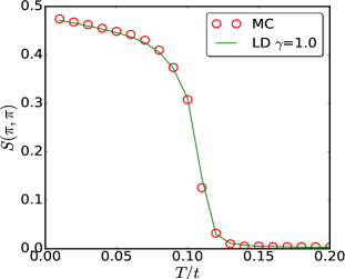
Fig.1 compares $S(\pi,\pi)$ from Langevin dynamics for various $\gamma$ values with that from MC annealing (red open circles). The agreement is excellent at $\gamma=1$, and generally good at the other $\gamma$ as well. The transition temperature $T_{c}\sim 0.12t$ is inferred from the onset of rise in both curves. The transition is in the Ising class, however there’s a quantitative reduction of structure factor in the low $T$ regime due to the continuous nature of the $x_{i}$ variable, absent in the Ising model. The dependence on $\gamma$ is weak, but higher $\gamma$ generally leads to better correspondence with equilibrium MC results.

III.2 $P(x)$ distributions

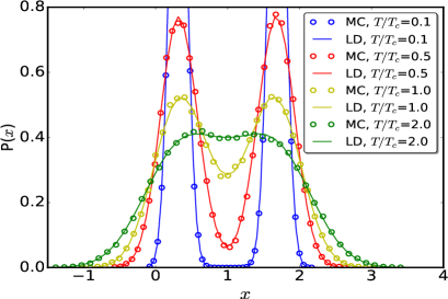
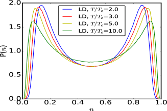
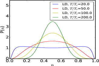
In Fig.2 we show the $P(x)$ obtained from a Monte Carlo calculation, compared to results from LD at $\gamma=1$. The dynamical method gives histograms quantitatively comparable to the MC results. We plot the distributions at four temperatures - $0,~{}0.5T_{c},~{}T_{c},~{}2T_{c}$. The solid lines are the Langevin data whereas open circles depict results from MC annealing. The agreement suggests that the two methods should predict the same ‘equal-time’ properties in equilibrium.

Figure 3: Top panels: Trajectories of nearest neighbour sites for part of the full time series. We see harmonic vibrations about equilibrium positions in the left figure. The fluctuation window increases considerably on heating ($0.5T_{c}$), featured in the right figure. Bottom panels: Corresponding Fourier mode trajectories at the same temperatures. The means are subtracted and trajectories shifted by a constant in the left figure ($0.1T_{c}$). The effect of anharmonicity is to reduce the mean $X(\pi,\pi)$ and visibly enhance fluctuations in both $(0,0)$ and $(\pi,\pi)$ modes.

   

 

Figure 4: Top row: False color maps of the power spectrum $|X({\bf q},\omega)|^{2}$ in the low temperature regime. The spectral intensities are plotted with the momentum trajectory $(0,0)\rightarrow(\pi,0)\rightarrow(\pi,\pi)\rightarrow(0,0)$ along the x-axis. Bottom row: Lineshapes at corresponding temperature points for three momentum points along the BZ diagonal: $(0,0)$, $(\pi/2,\pi/2)$ and $(\pi,\pi)$. All power spectra are normalized by $k_{B}T$.

IV Real time dynamics

We classify our results into four thermal regimes: (a) low temperature, $T\lesssim 0.6T_{c}$, where the dynamics is harmonic or mildly anharmonic, (b) the ‘critical’ window, $0.6T_{c}\lesssim T\lesssim 1.5T_{c}$, where thermal tunneling events dominate, (c) the ‘polaron liquid’ phase, $1.5T_{c}\lesssim T\lesssim 10T_{c}\sim T_{P}$, where the distortions and density still have a bimodal character but spatial correlations are only short range, and (d) the ‘polaron dissociated’ phase, $T\gtrsim T_{P}$, where we have essentially independent local oscillations. For each of these regimes we typically show some trajectories for the real space dynamics, time dependence of some Fourier modes, the power spectrum, and sometimes damping and dispersion scales extracted from the power spectrum.

IV.1 Harmonic and weakly anharmonic regime: $T\ll T_{c}$

IV.1.1 Real time trajectories

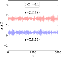
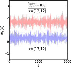
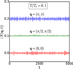
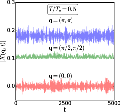
Fig.3 shows the time dependence of phonon variable both in real and momentum space at $T=0.1T_{c}$ and $T=0.5T_{c}$. The top left panel shows the trajectories $x_{\bf r}(t)$ at nearest neighbour sites, ${\bf r}=(12,12)\&(13,12)$ at $T=0.1T_{c}$, while the top right panel shows the same at $T=0.5T_{c}$. The $0<T<0.6T_{c}$ window roughly defines the ‘low temperature’ regime as we discuss below. The left panel shows small amplitude vibrations about mean distortions $\sim 0$ and $2$ respectively. The right panel shows a qualitative increase in fluctuation amplitude, retaining similar mean values.

The bottom panel depicts trajectories $|X({\bf q},t)|$ at three momenta along the Brillouin Zone (BZ) diagonal. The left panel is at $T=0.1T_{c}$, the right at $T=0.5T_{c}$. In the left panel we subtracted the mean values and shifted the curves by a constant ($0.1$) to aid visualization. The ${\bf q}=(0,0)$ and $(\pi,\pi)$ modes are seen to fluctuate more compared to $(\pi/2,\pi/2)$. In the right panel the mean $|X(\pi,\pi,t)|$ reduces. Oscillations are most prominent at $(\pi,\pi)$.

Figure 5: Fitting the dispersion $b({\bf q})$ using harmonic functions on the BZ at the lowest $T=0.1T_{c}$. We find that a nearest neighbour model is reasonable accurate in describing the dispersion of mode values. The blue open circles are extracted from the data, green solid line is the best fit with free parameters $K_{eff}$ and $J$ and the red dashed curve features RPA result computed using the perfect ordered state at zero $T$. The obtained fitting parameters are $K_{eff}=0.78$ and $J=0.09$, which denote the effective local stiffness and the nearest neighbour intersite coupling respectively.

Figure 6: Quantifying the effect of anharmonicity. Left: $\Delta\omega_{max}({\bf q},T)$: the difference of peak locations from that at $T=0$, and Right: the linewidth $\Gamma_{\bf q}(T)$. Results are for three characteristic momenta- $(0,0)$, $(\pi/2,\pi/2)$ and $(\pi,\pi)$. We see linear softening of mode values and an initially linear increase in damping for all momenta. Non-linear corrections take over in the latter as one raises the temperature.

IV.1.2 Power spectrum

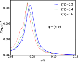
We turn now to the description of dynamics in terms of $|X({\bf q},\omega)|^{2}$. The top row of Fig.4 features the results in the low temperature regime. The maps are color coded in terms of varying intensity and the X-axis shows a momentum scan along the trajectory $(0,0)\rightarrow(\pi,0)\rightarrow(\pi,\pi)\rightarrow(0,0)$ in the 2D BZ. We have divided out all $|X({\bf q},\omega)|^{2}$ by $k_{B}T$.

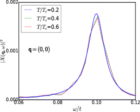
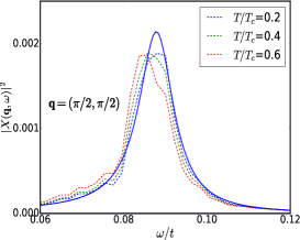
In the bottom panel, we’ve plotted the lineshapes at three characteristic momenta ($(0,0),(\pi/2,\pi/2),(\pi,\pi)$ in terms of their $T$ dependence. Here small changes are observed on increasing temperature as one goes from the harmonic to the anharmonic regime. The $(\pi,\pi)$ mode is most sensitive to this effect, whereas the lineshapes at BZ center don’t respond appreciably.

The asymptotically low temperature regime is understandable in terms of an effective harmonic model. The assumption is that the deviations of displacement fields from the checkerboard ordered ground state pattern are small. The most general distortion cost one can write to quadratic order is: $V^{(2)}_{eff}\approx\sum_{i,j}b_{ij}\Delta x_{i}\Delta x_{j}$, where the $\Delta x_{i}=x_{i}-x_{i}^{0}$, with $x_{i}^{0}$ being the distortion in the $T=0$ CO state. The resulting Langevin equation is linear in $\Delta x_{i}$, but spatially coupled, and can be solved by Fourier transformation. The $b_{ij}$ can be obtained from an expansion of the ground state energy, $b_{\bf q}$ is its Fourier transform. The power spectrum that emerges has the form:

$$|X({\bf q},\omega)|^{2} = \frac{2\gamma k_{B}T}{|f({\bf q},\omega)|^{2}}$$ (16)

$$f({\bf q},\omega)~{}~{} = (-M\omega^{2}+b_{\bf q}+i\gamma\omega)$$ (18)

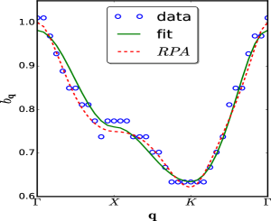
The dispersion, found by plotting the peak locations at the lowest $T=0.1t$, has been fitted in Fig.5 to obtain the coefficients of nearest and next-nearest neighbour contributions in $b_{\bf q}$. The fit parameters are $K_{eff}=0.78$ and $J=0.09$, respectively the local stiffness and the nearest neighbour coupling. The further neighbour contributions are significantly smaller, owing to the gap in density of states of the ordered state. The dispersion compares well with a ‘random phase approximation’ (RPA) calculation done on the $T=0$ CO background, using the static polarizability, $\Pi({\bf q},\omega=0)$.

Figure 7: Top panel: Trajectories of nearest neighbour sites for part of the full time series. We see ‘resident flips’ first appearing in the left figure ($0.9T_{c}$). The nearest neighbours switch in mean values and stay for tens of oscillation timescales. Moving to the actual $T_{c}$, featured in the right figure, we see more frequent exchange moves that ultimately leads to vanishing of $S(\pi,\pi)$. Bottom panel: Corresponding Fourier mode trajectories at the same temperatures. The mean values are retained and actual trajectories are shown without shifting, as opposed to the low $T$ figure. We see the special behaviour of the $(\pi,\pi)$ mode quite clearly near criticality. Large oscillations feature in the left figure while a reduction of mean value to near zero is visible at $T_{c}$.

   

  

Figure 8: Top row: Maps of the power spectrum $|X({\bf q},\omega)|^{2}$ in the vicinity of $T_{c}$. The spectral intensities are plotted with the momentum trajectory $(0,0)\rightarrow(\pi,0)\rightarrow(\pi,\pi)\rightarrow(0,0)$ along the x-axis. Bottom row: Lineshapes at corresponding temperature points for three momentum points along the BZ diagonal: $(0,0)$, $(\pi/2,\pi/2)$ and $(\pi,\pi)$. All power spectra are normalized by $k_{B}T$.

The departure from harmonic behaviour with increasing $T$ can be motivated by using a cubic term in the energy, below. The energy cost with cubic terms has a form: $V^{(3)}_{eff}=\sum_{ij}b_{ij}\Delta x_{i}\Delta x_{j}+\sum_{ijk}c_{ijk}\Delta x_{i}\Delta x_{j}\Delta x_{k}$ Fourier transforming the Langevin equation leads to

$$f({\bf q},\omega)X({\bf q},\omega)=\xi({\bf q},\omega)-\alpha({\bf q},\omega)$$

where $\alpha({\bf q},\omega)=\sum_{{\bf q}^{\prime},\omega^{\prime}}C_{{\bf q},{\bf q^{\prime}}}X({\bf q}-{\bf q}^{\prime},\omega-\omega^{\prime})X({\bf q}^{\prime},\omega^{\prime})$. This can be dealt with perturbatively by substituting the harmonic solution in the nonlinear term. One formulates the perturbation expansion in terms of the response function $\langle X({\bf q},\omega)\xi({\bf-q},-\omega)\rangle$. The Fourier transformed variable $X({\bf q},\omega)$ has an expansion in powers of the anharmonic coefficient. This has the first non-vanishing correction for the response function at second order, as odd order correlators of the noise vanish by symmetry.

Before averaging over the noise variable, one has all kinds of diagrams for the response function with cubic interaction vertices and ‘dangling legs’ of the noise. After taking the noise average, these legs connect up and one family of diagrams may be identified as the ‘RPA series’, which has repeated ‘bubbles’ arising as corrections to the free propagator. One can then selectively resum these contributions. The effective self-energy $\Sigma({\bf q},\omega)$ that emerges has the form:

$$\Sigma({\bf q},\omega)=\langle\sum_{{\bf q}^{\prime},\omega^{\prime}}\frac{\xi({\bf q}-{\bf q}^{\prime},\omega-\omega^{\prime})\xi({\bf q}^{\prime},\omega^{\prime})}{f({\bf q}-{\bf q}^{\prime},\omega-\omega^{\prime})f({\bf q}^{\prime},\omega^{\prime})}\rangle$$

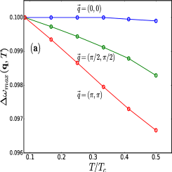
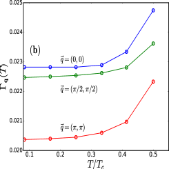
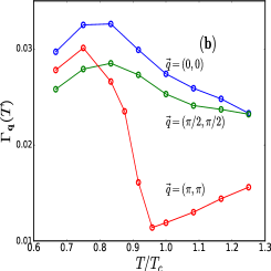
where angular brackets denote averaging over the noise variable. This is an $O(T)$ quantity at this level. The real and imaginary parts of this corrects the pole location and damping respectively, with the corrections varying linearly with $T$ for a fixed $\bf{q}$.

Fig.6 indicates that the frequency shift and increase in broadening indeed have a leading linear $T$ behaviour at low temperature. The damping features non-linear corrections in $T$ as one heats up, which arise from ‘stray flips’ (SF) which are large, isolated exchange of displacements on the lattice. The slope of the linear part is of course ${\bf q}$ dependent and the nature of this dependence is monotonic along the BZ diaginal.

Figure 9: Fits to extract the mean frequencies ($\bar{\omega}$) and standard deviations ($\Delta\omega$) as functions of temperature. The left panel features mean curves, showing an overall softening trend that’s most prominent at $(\pi,\pi)$. The right panel features damping rates, where a non-monotonicity is seen in the thermal behaviour. At $T_{c}$, the $(\pi,\pi)$ mode is again sharp.

     

Figure 10: Top panel: Growth of a large domain is shown through taking the actual configurations and subtracting out the prevalent checkerboard pattern $C$. Bluish regions indicate perfect order alla $C$ and red regions denote opposite pattern of checkerboard ordering $C^{\prime}$. The white areas are indicative of boundaries between these two patterns. Time is measured in units of $\tau_{0}$, the bare oscillation timescale. Bottom panel: The instantaneous structure factor $S(\pi,\pi,t)$ shown across the time interval of domain growth. Dominant order alla $C$ or $C^{\prime}$ result in increased value, while in the middle panel we observe a near zero value due to almost equal size of the two domains.

IV.2 Critical fluctuations: $T\sim T_{c}$

IV.2.1 Real time trajectories

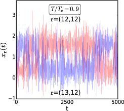
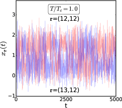
The trajectories in both real and momentum space for this regime are shown in Fig.7. The top row depicts nearest neighbour displacement time series. New events show up compared to low $T$, in the form of ‘exchange moves’ between large and small distortions. The left figure ($T/T_{c}=0.9$) shows a clean version of what may be called a ‘resident flip’ (RF), where the exchanged distortions don’t flip back within a short ($\sim 5-10\tau_{0}$) timescale. Moving closer to the actual $T_{c}$, their frequency increases. These events have associated spatial correlations as well, which trigger domain growth and shrinkage, as discussed later. Ultimately, these lead to destruction of order as a whole.

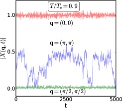
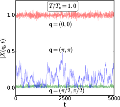
The bottom row of Fig.7 shows trajectories of different momentum modes. This time the mean values are shown without shifts. As before, we observe the benign nature of $(0,0)$ and $(\pi/2,\pi/2)$ modes. The $(\pi,\pi)$ mode, however, features large oscillations just before $T_{c}$, whose mean value drops rapidly on approaching criticality. The dynamical event responsible for this is domain growths, taking place over the full lattice. We will discuss this later.

IV.2.2 Power spectrum

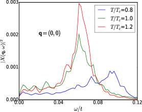
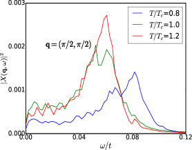
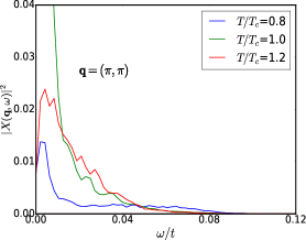
Moving to the frequency dependent indicators, far richer behaviour is seen here compared to low temperatures. The top row of Fig.8 depicts spectral maps of $|X({\bf q},\omega)|^{2}$. In the leftmost figure ($T=0.7T_{c}$), a faint tail is seen emerging near $(\pi,\pi)$. A more complete weight transfer is observed in the middle panel ($T=0.8T_{c}$). This originates from ‘exchange moves’ discussed before in the context of trajectories. They have an associated timescale that is much larger ($\sim 100$ times) than the bare oscillation period.

Low energy spectral weight arises from these moves. If one tracks the trajectories long enough, these should be present at even lower $T$. However, there these events are too rare to have any appreciable impact on the frequency response of the system as a whole. Stray flips (SF) start occuring around $0.6T_{c}$, whereas RF’s discussed before only show up around $0.9T_{c}$. The spectrum at criticality (right panel) has a different dispersive character compared to lower $T$ and is considerably more broad around $(\pi,\pi)$.

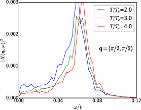
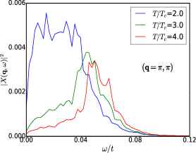
The lineshapes at three characteristic momenta $(0,0)$, $(\pi/2,\pi/2)$ and $(\pi,\pi)$ features in the bottom row of Fig.8. A gradual spectral weight transfer to lower frequencies is observed in the first two on heating close to $T_{c}$, whereas a dramatic near-zero frequency weight develops at $(\pi,\pi)$. The intensity also, even after being divided out by a factor of $k_{B}T$, is $\sim 10$ times here at $T_{c}$.

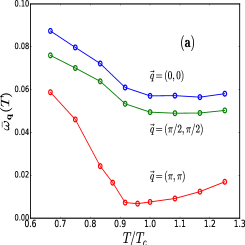
In Fig.9, we’ve shown mean frequencies (left panel) and standard deviations (right panel) across the chosen trajectory in BZ in this regime. The softening at the BZ boundary is quite prominent on approaching $T_{c}$. The overall branch also changes its character compared to low $T$. In the dampings, a non-monotonic trend is seen, also most prominent at $(\pi,\pi)$. The width of the spectrum at this momentum is actually resolution limited, rather than $\gamma$ limited. Hence, this is an universal feature, irrespective of microscopic details.

IV.2.3 Domain dynamics near $T_{c}$

The ground state of the present problem is $(\pi,\pi)$ ordered, which corresponds to a checkerboard pattern. However, there exists two energetically degenerate patterns, related to each other by a $Z_{2}$ transformation. We call them C and C’. During the time evolution there are two kinds of forces acting on the each lattice site. One is the systematic part of the force ($g\bar{n}_{i}-Kx_{i}$). This depends on the $\{x_{i}\}$ configuration at the given instant. The other is the thermal noise. At zero temperature, if we create a small defect in the lattice (a small domain of C in C’ or vice versa), it exterts a force on its neighbours, trying to convert them into C and hence growing the domain. These events are rare at low temperature.

Figure 11: Left: Trajectories of nearest neighbour sites for part of the full time series. We see flip moves merging with large amplitude oscillations. This leads to broad but unimodal power spectra in this regime. Right: Corresponding Fourier mode trajectories at the same temperatures. The mean values are retained and actual trajectories are shown without shifting, as opposed to the low $T$ figure. Both the $(\pi/2,\pi/2)$ and $(\pi,\pi)$ trajectories oscillate above zero, indicating loss of spatial correlations in the dynamics.

   

Figure 12: Top row: False color maps of the power spectrum $|X({\bf q},\omega)|^{2}$ in the disordered polaron liquid regime. The spectral intensities are plotted with the momentum trajectory $(0,0)\rightarrow(\pi,0)\rightarrow(\pi,\pi)\rightarrow(0,0)$ along the x-axis. Bottom row: Lineshapes at corresponding temperature points for three momentum points along the BZ diagonal: $(0,0)$, $(\pi/2,\pi/2)$ and $(\pi,\pi)$. All power spectra are normalized by $k_{B}T$.

At temperatures $\sim 0.5T_{c}$ there are considerable amplitude fluctuations about mean values at different sites. Also, large kicks cause ‘exchange moves’ or ‘flips’. However, only stray flips (SF) could be found (the defect stays only for $\sim\tau_{0}$ time). This happens because at low $T$ the effective potential for two sites in an otherwise frozen background has one deep minimum and one very shallow minimum (separated by $g/K$). Hence the difference in distortions can’t settle on a ‘flipped’ value and resident flips (RF, flips that stay for $\sim 100\tau_{0}$) cannot happen. As temperature increases ($\sim 0.8T_{c}$) the amplitude fluctuations of $x_{i}$’s increase and SF’s become more frequent. When an SF creates a defect and its neighborhood has a small difference in $x_{i}$’s, the force that the defect exerts on the neighbourhood might be enough to create spatially correlated flips, causing a growth of the domain.

Figure 13: Top panel: the distribution of local density $P(n)$ showing distinct bimodal features till $\sim 10T_{c}$. This means there’s a large region in temperature where polarons are present in the lattice, but there’s no global ordering. Bottom panel: Snapshots from time evolution at $T=3.0T_{c}$. One sees dynamic patterns of short-range correlated polarons, hinting a non-trivial spatial structure.

In Fig.10, we depict a domain growth event as a function of time from our data at $T/T_{c}=0.9$. The bluish regions depict ‘C’ kind of order, which dominates initially. However, with increasing time, the opposite pattern C’ tries to grow from within and the structure factor $S(\pi,\pi,t)$ decreases as a consequence. In the middle, we see a low structure factor where two kinds of domains are almost equally present. Later, the C’ order encompasses the lattice and $S(\pi,\pi,t)$ grows again. These ‘domain oscillations’ typically take place over a large ($\sim 500\tau_{0}$) timescale.

IV.3 Polaron liquid: $T_{c}\ll T<T_{P}$

In this regime long-range order is lost but there are short-range correlations still prevalent amongst large distortions. There is no obvious small parameter, or a universal phenomenology as in the critical regime.

Figure 14: False color maps of the power spectrum $|X({\bf q},\omega)|^{2}$ in the high $T$ regime. The spectral intensities are plotted with the momentum trajectory $(0,0)\rightarrow(\pi,0)\rightarrow(\pi,\pi)\rightarrow(0,0)$ along the x-axis.

IV.3.1 Real time trajectories

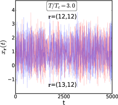
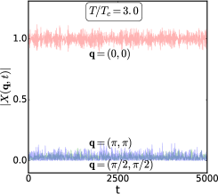
The left panel of Fig.11 features real space trajectories on nearest neighbours at $T=3.0T_{c}$, where one sees a merger of large oscillations and flip moves. The corresponding momentum trajectories at this temperature are all featureless, as observed in the right panel.

IV.3.2 Power spectrum

The power spectra (top panel in Fig.12) display a mildly dispersive band with pronounced softening and broadening near $(\pi,\pi)$. The dip gradually reduces on heating up, signifying loss of intersite correlations. There’s also a mild stiffening of the branch as a whole with increasing $T$. On heating up even further, one sees the branch lose dispersion at $\sim 10T_{c}$. The broadening also becomes $\gamma$ limited eventually. This signifies that the effective Hamiltonian for the oscillators first reduces to a local one and then the anharmonicities vanish at asymptotically high $T$.

The lineshapes at specific momenta corroborate the conclusions drawn above. At lower $T$, the damping is highest at the BZ corner. The mode values shift on heating up. There’s a quantitative reduction in damping on heating for all momenta, the most noticeable being $(\pi,\pi)$.

The corresponding density distributions and snaphots are highlighted in Fig.13. In the top panel, we do see prominent bimodality for an extended range of temperatures ($2T_{c}-10T_{c}$). This is indicative of the fact that polarons and their short-range correlations (shown in the bottom panel) dictate the physics in this regime.

IV.4 Polaron dissociated phase: $T\gtrsim T_{P}$

In the high $T$ regime, the power spectrum gradually loses dispersive features and is broadened compared to its low $T$ counterpart. Intuitively, these features can be explained using an effective Hamiltonian with a nonlinear local term and a nearest neighbour harmonic part for the $x_{i}$ field. The local term may be derived by tracing out electrons from a single site Holstein problem. The nearest neighbour coefficient is of order $J\sim\frac{t^{2}}{E_{p}}$. The dimensionless form of the full Langevin equation reads-

$$\frac{d^{2}X_{i}}{d\tau^{2}}=-\gamma^{\prime}\frac{dX_{i}}{d\tau}-X_{i}+\langle n_{i}\rangle+\sqrt{\frac{k_{B}T}{E_{p}}}\eta_{i}$$ (19)

where $\gamma^{\prime}=\gamma/M\omega_{0}$, $\tau=\tau_{0}t$ and $X_{i}=(g/K)x_{i}$. The noise correlator is given by-

$$\langle\eta_{i}(\tau)\eta_{j}(\tau^{\prime})\rangle=\gamma^{\prime}\delta_{ij}\delta(\tau-\tau^{\prime})$$ (20)

Figure 15: Effective stiffness ($K_{eff}$) plotted against $1/T$ in the asymptotically high $T$ regime. A linear fit (consistent with a high $T$ expansion) is in fairly good agreement with the data. Ultimately, for small $1/T$, one gets back to the bare stiffness value $K=1$.

Figure 16: $P(n)$ and spatial character in the ‘polaron dissociated’ phase. The top panel depicts a broad distribution at the lowest temperature shown ($T/T_{c}=20.0$) gradually sharpening to a nearly gaussian distribution with mean $n=0.5$ at very high temperature ($T/T_{c}=200.0$). The spatial character shows ‘melted’ polarons, which don’t have any interesting dynamics.

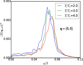
At asymptotically high temperature, $T\gg E_{p}$, the density becomes a local, linear function of $X_{i}$ and the corresponding power spectrum becomes identical to that of a single harmonic oscillator with a renormalized frequency. This frequency approaches the bare value at asymptotically high temperature. On lowering $T$, higher order corrections in $\beta E_{p}$ feature in the $<n_{i}>$. We have a linear ($O(\beta E_{p}$)) correction to the bare stiffness featuring first, and then a higher order ($O(\beta^{3}t^{2}E_{p})$) intersite correction which gives rise to ‘dispersion’ at lower $T$. In Fig.14, the power spectra in this regime are featured, which ceases to show dispersive features and only exhibits gradual band tightening, with reduction in damping as one heats up.

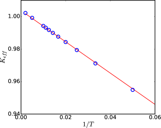
In Fig.15, we fit the effective stiffness, calculated from the $P(x)$ distributions against $1/T$. One expects a linear variation from an analytic high $T$ expansion, which is borne out by the actual data.

The density distribution and snapshots from dynamics in this regime are shown in the top and bottom panels of Fig.16. respectively. The distributions converge to a gaussian at large enough $T$, with a mean $n=0.5$ and width proportional to $\sqrt{T}$. The snapshots exhibit ‘melted’ polarons, which are represented as greyish regions.

Figure 17: (a)  The structure factor $(\pi,\pi)$ at $T=0.2T_{c}$ for three different $\gamma$ values- $(0.1,0.5,1.0)$. The $\gamma=0.1$ result features a slightly higher $T_{c}$ compared to the other two. There’s a ‘saturation’ at higher $\gamma$, whose results coincide with one another. (b)  The ($\pi,\pi$) lineshape in the low $T$ harmonic regime. The broadening is observed to increase proportionately with $\gamma$, as expected from the harmonic oscillator result. (c)  The $(\pi,\pi)$ lineshapes at $T_{c}$ plotted on a logarithmic scale. The $\gamma$ variation is significantly suppressed in this critical regime.

  

Figure 18: (a) The structure factor $S(\pi,\pi)$ characterizing order-disorder transition for three different sizes- $(12\times 12,16\times 16,24\times 24)$. The $\gamma$ value is $1.0$ for all of them. We see a mildly sharper transition for the largest size. (b) Power spectra at $(\pi,\pi)$ for different sizes. The character is similar for all the profiles, with a growing weight near zero frequency for larger sizes.

V Discussion

V.1 Computational checks

V.1.1 Dependence of results on $\gamma$ choice

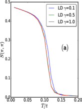
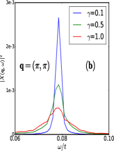
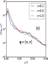
The stucture factors for different $\gamma$ values have an overall similarity. The lower $\gamma=0.1$ gives a slightly higher $T_{c}$. The $\gamma=0.5$ and $\gamma=1.0$ curves lay on top of each other, signifying the insensitivity of the system’s equal-time properties on this parameter (shown in Fig.17(a)). However, we comment that if one uses a much higher $\gamma$, the problem ceases to have a correspondence with the physical Holstein model and becomes overdamped. To establish the dependence of power spectra on $\gamma$, we look at two different temperature regimes- i) the low $T$ harmonic regime and ii) the critical regime ($T\sim T_{c}$). The observations are featured in Figs.17(a) and 17(b) respectively. In the former, increasing $\gamma$ by a decade (0.1-1.0) has a proportionate impact on the broadening of the $(\pi,\pi)$ lineshape. This is expected from the analytic form of the power spectrum, as discussed in subsection A of the results section. On the other hand, near $T_{c}$, the dependence on $\gamma$ is feeble. We have superposed the $(\pi,\pi)$ lineshapes on a logarithmic scale for three different $\gamma$ values to show this. The conclusion is that the critical behaviour is universal and doesn’t depend crucially on microscopically generated dissipation scales.

V.1.2 Size dependence

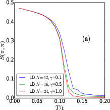
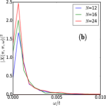
We have checked size dependence of the $S(\pi,\pi)$, which characterises the order-disorder transition and the $(\pi,\pi)$ lineshapes at criticality. The results are displayed in Figs.18(a) and 18(b) respectively. The former shows a sharper transition as we go to bigger sizes ($16\times 16$ to $24\times 24$), as expected. The low to intermediate temperature behaviour, governed by linear phonon excitations, is very similar for all sizes. The latter quantity has a width that is basically resolution limited for all sizes. The weight at ‘near-zero’ frequency increases nominally with size. We expect an infinitely sharp peak at zero frequency in the thermodynamic limit.

V.2 Simple models for the different regimes

Figure 19: Effective potential for the ‘embedded two-site’ problem plotted against the difference in displacements $x=(x_{1}-x_{2})$ of the two sites. The background order is a perfect checkerboard with distortions $0$ and $g/K$ respectively. The potential is obtained by keeping $x_{1}+x_{2}$ fixed, which ensures number conservation locally. The look is that of an asymmetric double well with an extremely shallow second minimum. The oscillation freqeuncy at the harmonic level about the lower well is $0.054$ and that about the overall profile (relevant at very high temperature) is $0.069$. The potential is indeed harmonic at large range. The splitting between the two minima is $\Delta=0.38$.

Figure 20: (a) Spectra of the model problem ($|(x_{1}-x_{2})(\omega)|^{2})$ compared with (b) the actual power spectrum of the full problem at $(\pi,\pi)$. A visual similarity is apparent for both the low and high $T$ regimes. Frequencies are scaled with respect to $\omega_{osc,2}$ in the former and $\Omega$ in the latter case. Temperatures are featured in units of $\Delta$ for the model problem and $T_{c}$ for the full problem.

V.2.1 Non critical behaviour

We attempted an explanation of the features found in the power spectrum of wavevectors near the zone boundary through a single variable toy model. It misses the collective critical dynamics but gives a fairly good account of ‘beyond harmonic’ physics at low to intermediate temperatures and also the high $T$ regime.

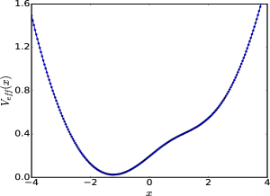
The model problem constructed is a two-site Holstein dynamics embedded in the background of the $T=0$ mean-field state, which is $(\pi,\pi)$ ordered. The sum of coordinates $(x_{1}+x_{2})$ is held fixed, to ensure particle density conservation, while $(x_{1}-x_{2})$ is varied to first generate an effective potential numerically. Then, the dynamics of the ‘collective coordinate’ is studied within this potential. Although, in the real problem, there’s no density conservation locally, the present simplification is a good enough approximation at least for $T<T_{c}$.

The look of this effective potential (shown in Fig.19) is that of an asymmetric double well at low values of $(x_{1}-x_{2})$, with a very shallow second well. The difference in well depths is due to correlation energies arising from the background order. Hence, the energy splitting $\Delta$ between the two minima is comparable to $T_{c}$ in the actual problem. At asymptotically large values of $(x_{1}-x_{2})$, the potential is harmonic, whose stiffness can be extracted numerically. Hence, the profile can’t be fitted to any polynomial function over the full range.

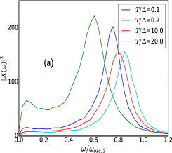
The dynamics features three timescales- (i) the oscillation time about the deeper well ($\tau_{osc,1}$), where the initial condition is chosen to lie, (ii) $\tau_{flip}$, for excursions to the shallower well and (iii) the oscillation time about the overall potential profile ($\tau_{osc,2}$). These become accessed gradually as one increases $T$. The frequency scales corresponding to (i) and (iii) are 0.054 and 0.069 respectively.

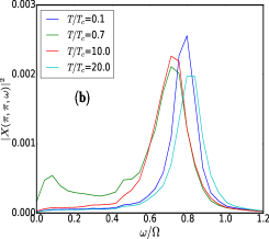
We’ve analyzed the power spectrum of the difference coordinate $|(x_{1}-x_{2})(\omega)|^{2}$ for various values of the scaled temperature $T/\Delta$, where $\Delta$ is the energy splitting between two wells. The frequencies are scaled with respect to $\Omega$ (the bare oscillation frequency) in the real problem and $\omega_{osc,2}$ in the model situation. Fig.20 (panels (a) and (b)) shows the result. Fig.20(a) is for the model problem, whereas 20(b) is for the actual dynamics. The gross behaviour is simple- at low enough $T/\Delta$, harmonic dynamics about the deeper well is observed, with the characteristic frequency related to its stiffness. At slightly higher temperatures, anharmonic effects result in well shift and quantitatively larger damping. Then, the flips to the shallower well start showing up, with $\tau_{flip}\gg\tau_{osc,1}$. This results in an accumulation of spectral weight near zero frequency. For $T/\Delta\gg 1$, the oscillations take place about the overall profile. The peak shifts towards a frequency consistent with the corresponding stiffness and damping again becomes $\gamma$ limited.

V.2.2 Critical behaviour

We attempted to understand the critical behaviour in terms of dynamics of an Ising model with nearest neighbour AF coupling. Since this is a discrete variable model, the dynamics was designed in terms of the ‘sign’ of the evolved degree of freedom. The equation of motion (in discrete form) is-

$$H = J\sum_{<ij>}S_{i}S_{j}$$ (21)

$$S_{i,t_{n+1}} = sgn(S_{i,t_{n}}-\epsilon*\frac{\partial H}{\partial S_{i}}+\sqrt{\epsilon}*\eta_{i,t_{n}})$$

The parameters for this problem were: $J=1$ and $\epsilon=0.01$. The noise has the properties-

$$\langle\xi_{i}(t_{n})\rangle~{}~{}~{}~{} = 0$$ (22)

$$\langle\xi_{i}(t_{n})\xi_{j}(t_{m})\rangle = 2k_{B}T\delta_{ij}\delta_{nm}$$

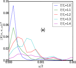
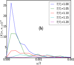
This can be interpreted as an overdamped Langevin equation, from which the critical dynamics can be extracted along with the thermodynamics. The power spectrum of this model at $(\pi,\pi)$ has a Lorentzian profile about zero, whose width collapses as one tunes the temperature near $T_{c}$ ($\sim 2.2J$) from above. At higher $T$, one observes gradual broadening, related to the reduction of correlation length. A direct comparison of the lineshapes between this model and the real problem at $(\pi,\pi)$ is shown in Figs.21(a) and 21(b). The temperatures are normalized by the respective $T_{c}$ scales.

Figure 21: (a) Spectra of the Ising problem compared to the actual power spectra (b) of the full problem at $(\pi,\pi)$. A visual similarity is apparent close to $T_{c}$, where other details are irrelevant. Frequencies are scaled with respect to $J$ in the former and $t$ in the latter case. Temperatures are featured in units of $T_{c}$ for the respective problems.

The coarse-grained, continuum limit of the AF Ising system with a conserved magnetization density, relevant to the present Holstein model, falls under Model B amongst the dynamical universality classes, introduced by Halperin and Hohenberghohenberg . This model in the Gaussian limit ($T\gg T_{c}$) can be solved analytically to yield a Lorentzian power spectrum, whose width collapses on approaching $T_{c}$ from above.

Let $S(q,\omega)$ be the coarse grained spin field. The power spectrum is obtained by multiplying two factors of this field and averaging over the noise, which gives-

$$\langle S(q,\omega)S(q^{\prime},\omega^{\prime})\rangle = C(q,\omega)(2\pi)^{d+1}\delta(q+q^{\prime})\delta(\omega+\omega^{\prime})$$ (24)

$$C(q,\omega) = \frac{2k_{B}TDq^{2}}{\omega^{2}+(Dq^{2}(r+q^{2}))^{2}}$$

This profile is a Lorentzian and has width that is almost $Dq^{2}r$ for $T\gg T_{c}$ and almost $Dq^{4}$ for $T\sim T_{c}$. Hence, we have a diminishing width (strictly zero for $q\rightarrow 0$) as one approaches $T_{c}$ from above.

V.3 Experimental signature

Several recent experiments suggest an anomalous behaviour of phonon dispersion and damping across a thermal transition in manganitesweber1 ; weber2 ; weber3 . The inelastic neutron scattering data reveals that phonons broaden and soften considerably as one makes a transition from a ferromagnetically ordered, homogeneous ground state to a paramagnetic insulator with short-range correlated small polarons. In the insulating state, reduction of states near the Fermi level again causes a decrease in both the softening and damping. While there are additional magnetic degrees of freedom which are relevant in these materials, we believe our framework can be generalized to give a theoretical explanation of these data. Part of our ongoing work is to compute phonon properties using Langevin equation on the doped Holstein model, to avoid charge ordering physics. If one couples the conduction electrons in this to ‘local moments’ with a double exchange coupling, the resulting system is a reasonable model for doped manganites. We plan to study the phonon dynamics there.

V.4 Future problems

V.4.1 Going beyond thermal noise

The present paper is based on numerical calculations done with a white, memory- less noise field. While this may be a good enough approximation for $\omega/k_{B}T\ll 1$, to estimate the low $T$ behaviour, one has to include memory effects encoded within $[\Pi]_{ij}^{K}(\omega)$. This is easier said than done, but the lowest order modification will be to introduce a ‘thermal correlation time’ that goes to zero in the high $T$ limit. This will also make the damping term non-local in time with the same $\tau_{th}$ timescale. The calculation of such a characteristic time has to be done by calculating the polarizability in the adiabatic approximation. This extension of the present scheme will give rise to an equation which is more complicated to solve numerically. But, it should contain more quantum fluctuation effects built into it which are important at low $T<<\omega$. The physics of harmonic phonons will be better captured, as regards dispersion and momentum dependent damping. Moreover, we hope barrier tunneling events which restore translation symmetry for doped systems will also be accessible.

V.4.2 Acoustic phonons, multiple atomic species

The present study contains a single optical phonon mode coupled to conduction electrons. To model a more realistic physical system, one has to include additional vibrational modes like acoustic phonons. This requires a term with intersite couplings at the non-interacting level. One may readily introduce such terms in the instantaeous Hamiltonian of the present scheme. Moreover, multiple atomic species with different masses can be also brought in within the same basic equation. This amounts to just changing the inertia term and has a bearing on the phonon scattering rates.

V.4.3 Impact of disorder

Real materials like manganites always have intrinsic disorder effects arising from a substitutional origin. One may introduce potential disorder in the present scheme directly through the Hamiltonian. Moreover, one can also put in random mass terms (taken from a binary distribution) to mimic a disordered medium. The main effect should be on the phonon damping, which will increase substantially even at low temperature. Disorder will also suppress quantum tunneling effects making our strategy more justifiable at low enough temperatures.

VI Conclusions

We have studied the real time dynamics of the Holstein model at half filling using a Langevin approach. This exploits the smallness of the bare phonon energy with respect to the electron hopping to simplify the ‘force’ acting on the phonon degrees of freedom. Using exact diagonalisation of the electron problem and Newtonian evolution of the stochastic equation we establish the phonon dynamics from the low temperature charge ordered phase, through the critical region, into the high temperature polaron liquid phase. This reveals non monotonic variation in both the mean energy $\omega_{\bf q}$ and damping $\Gamma_{\bf q}$ of the phonon modes with respect to temperature. This approach, building in large amplitude dynamical fluctuations, can help address a wide variety of finite temperature phonon problems including issues of thermal transport. Using an auxiliary field approach it can also approach the dynamics of other correlated electron problems.

We acknowledge use of the High Performance Computing Facility at HRI.

References

- [1] J. M. Ziman, Electrons and phonons, Oxford University Press (2001).
- [2] J. Bardeen, L.N. Cooper, and J.R.Schrieffer, Phys. Rev. 108, 1175 (1957).
- [3] G. Gruner, Rev. Mod. Phys. 60, 1129 (1988).
- [4] David Emin, Polarons, Cambridge University Press (2012).
- [5] A.S. Alexandrov, Polarons in Advanced Materials, Springer (2007).
- [6] Y. Tokura, Physics Today, 56, 7, 50 (2003).
- [7] Masatoshi Imada, Atsushi Fujimori, and Yoshinori Tokura, Rev. Mod. Phys., 70, 1039 (1998).
- [8] Y.Tokura, Colossal Magnetoresistive Oxides, CRC Press (2000).
- [9] A.S. Alexandrov and N.F. Mott, Polarons and Bipolarons, World Scientific, Singapore (1995).
- [10] Stefan Blawid and Andrew J. Millis, Phys. Rev. B, 63, 115114 (2001).
- [11] S.W. Lovesey ed., Dynamics of Solids and Liquids by Neutron Scattering , Springer (1977).
- [12] N. Mannella, W.L. Yang, X.J. Zhou, H. Zheng, J.F. Mitchell, J.Zaanen, T.P. Devereaux, N. Nagaosa, Z. Hussain and Z.-X. Shen, Nature, 438, 474 (2005).
- [13] Michael Sentef, Alexander F. Kemper, Brian Moritz, James K. Freericks, Zhi-Xun Shen, and Thomas O. Devereaux, Phys. Rev. X, 3, 041033 (2013).
- [14] P. Bruesch, Phonons:Theory and Experiments, Vols. I-III, Springer (1982).
- [15] R. Blankenbecler, D.J. Scalapino, and R.L. Sugar, Phys. Rev. D 24, 8 (1981).
- [16] A. Georges, G. Koliar, W. Krauth, and M.J. Rozenberg, Rev. Mod. Phys. 68, 13 (1996).
- [17] F. Weber, N. Aliouane, H. Zheng, J.F. Mitchell, D.N. Argyriou, and D.Reznik, Nature Materials 8, 798 (2009).
- [18] F. Weber, S. Rosenkranz, J.-P. Castellan, R. Osborn, H. Zheng, J.F. Mitchell, Y. Chen, Songxue Chi, J. W. Lynn, and D. Reznik, Phys. Rev. Lett. 107, 207202 (2011).
- [19] M. Maschek, D. Lamago, J.-P. Castellan, A. Bosak, D. Reznik, and F. Weber, Phys. Rev. B 93, 045112 (2016).
- [20] C.E. Creffield, G. Sangiovanni, and M. Capone, Eur. Phys. J. B 44, 175 (2005).
- [21] M Hohenadler, H Fehske, and F F Assaad, Phys. Rev. B 83, 115105 (2011).
- [22] J. Loos, M. Hohenadler, A. Alvermann and H. Fehske, J. Phys.: Condens. Matter 18, 7299 (2006).
- [23] D. Meyer, A.C. Hewson, and R. Bulla, Phys. Rev. Lett. 89, 196401 (2002).
- [24] Stefan Blawid, Andreas Deppeler, and A.J. Millis, Phys. Rev. B 67, 165105 (2003).
- [25] A. Kamenev, Field Theory of Non-Equilibrium Systems, CUP (2011).
- [26] D. Mozyrsky, M.B. Hastings, and I. Martin, Phys. Rev. B 73, 035104 (2006).
- [27] Alex Zazunov and Reinhold Egger, Phys. Rev. B 81, 014508 (2010).
- [28] Jing-Tao Lu, Mads Brandbyge, Per Hedegard, Tchavdar N. Todorov, and Daniel Dundas, Phys. Rev. B 85, 245444 (2012).
- [29] P.C. Hohenberg and B.I. Halperin, Rev. Mod. Phys. 49, 3 (1977).
- [30] Gia-Wei Chern, Kipton Barros, Zhentao Wang, Hidemaro Suwa and Cristian D. Batista, Phys. Rev. B 97, 035120 (2018).