Augmented Autoencoders: Implicit 3D Orientation Learning for 6D Object Detection

Abstract

We propose a real-time RGB-based pipeline for object detection and 6D pose estimation. Our novel 3D orientation estimation is based on a variant of the Denoising Autoencoder that is trained on simulated views of a 3D model using Domain Randomization.

This so-called Augmented Autoencoder has several advantages over existing methods: It does not require real, pose-annotated training data, generalizes to various test sensors and inherently handles object and view symmetries. Instead of learning an explicit mapping from input images to object poses, it provides an implicit representation of object orientations defined by samples in a latent space. Our pipeline achieves state-of-the-art performance on the T-LESS dataset both in the RGB and RGB-D domain. We also evaluate on the LineMOD dataset where we can compete with other synthetically trained approaches.

We further increase performance by correcting 3D orientation estimates to account for perspective errors when the object deviates from the image center and show extended results. Our code is available here

1 Introduction

One of the most important components of modern computer vision systems for applications such as mobile robotic manipulation and augmented reality is a reliable and fast 6D object detection module. Although, there are very encouraging recent results from Xiang et al. (2017); Kehl et al. (2017); Hodaň et al. (2017); Wohlhart and Lepetit (2015); Vidal et al. (2018); Hinterstoisser et al. (2016); Tremblay et al. (2018), a general, easily applicable, robust and fast solution is not available, yet. The reasons for this are manifold. First and foremost, current solutions are often not robust enough against typical challenges such as object occlusions, different kinds of background clutter, and dynamic changes of the environment. Second, existing methods often require certain object properties such as enough textural surface structure or an asymmetric shape to avoid confusions. And finally, current systems are not efficient in terms of run-time and in the amount and type of annotated training data they require.

Figure 1: Our full 6D Object Detection pipeline: after detecting an object (2D Object Detector), the object is quadratically cropped and forwarded into the proposed Augmented Autoencoder. In the next step, the bounding box scale ratio at the estimated 3D orientation $\hat{R^{\prime}}_{obj2cam}$ is used to compute the 3D translation $\hat{t}_{obj2cam}$. The resulting euclidean transformation $\hat{H^{\prime}}_{obj2cam}\in\mathcal{R}^{4x4}$ already shows promising results as presented in Sundermeyer et al. (2018), however it still lacks of accuracy given a translation in the image plane towards the borders. Therefore, the pipeline is extended by the Perspective Correction block which addresses this problem and results in more accurate 6D pose estimates $\hat{H}_{obj2cam}$ for objects which are not located in the image center. Additionally, given depth data, the result can be further refined ($\hat{H}_{obj2cam}^{(refined)}$) by applying an Iterative Closest Point post-processing (bottom).

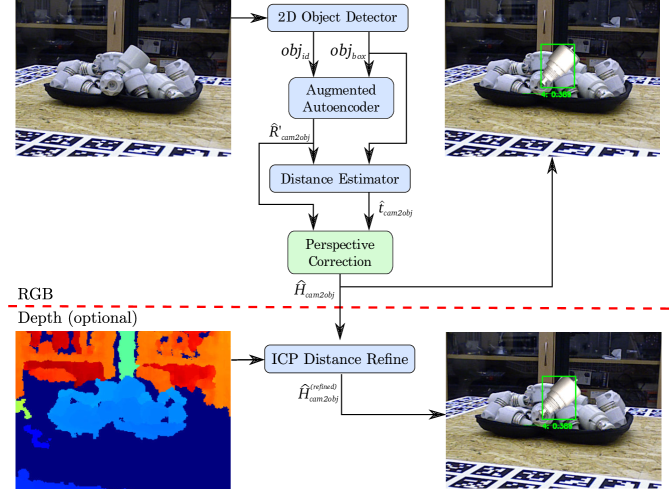
Therefore, we propose a novel approach that directly addresses these issues. Concretely, our method operates on single RGB images, which significantly increases the usability as no depth information is required. We note though that depth maps may be incorporated optionally to refine the estimation. As a first step, we build upon state-of-the-art 2D Object Detectors of (Liu et al. (2016); Lin et al. (2018)) which provide object bounding boxes and identifiers. On the resulting scene crops, we employ our novel 3D orientation estimation algorithm, which is based on a previously trained deep network architecture. While deep networks are also used in existing approaches, our approach differs in that we do not explicitly learn from 3D pose annotations during training. Instead, we implicitly learn representations from rendered 3D model views. This is accomplished by training a generalized version of the Denoising Autoencoder from Vincent et al. (2010), that we call ’Augmented Autoencoder (AAE)’, using a novel Domain Randomization strategy. Our approach has several advantages: First, since the training is independent from concrete representations of object orientations within $SO(3)$ (e.g. quaternions), we can handle ambiguous poses caused by symmetric views because we avoid one-to-many mappings from images to orientations. Second, we learn representations that specifically encode 3D orientations while achieving robustness against occlusion, cluttered backgrounds and generalizing to different environments and test sensors. Finally, the AAE does not require any real pose-annotated training data. Instead, it is trained to encode 3D model views in a self-supervised way, overcoming the need of a large pose-annotated dataset. A schematic overview of the approach based on Sundermeyer et al. (2018) is shown in Fig 1.

2 Related Work

Depth-based methods (e.g. using Point Pair Features (PPF) from Vidal et al. (2018); Hinterstoisser et al. (2016)) have shown robust pose estimation performance on multiple datasets, winning the SIXD challenge (Hodan, 2017; Hodan et al., 2018). However, they usually rely on the computationally expensive evaluation of many pose hypotheses and do not take into account any high level features. Furthermore, existing depth sensors are often more sensitive to sunlight or specular object surfaces than RGB cameras.

Convolutional Neural Networks (CNNs) have revolutionized 2D object detection from RGB images (Ren et al., 2015; Liu et al., 2016; Lin et al., 2018). But, in comparison to 2D bounding box annotation, the effort of labeling real images with full 6D object poses is magnitudes higher, requires expert knowledge and a complex setup (Hodaň et al., 2017).

Nevertheless, the majority of learning-based pose estimation methods, namely Tekin et al. (2017); Wohlhart and Lepetit (2015); Brachmann et al. (2016); Rad and Lepetit (2017); Xiang et al. (2017), use real labeled images that you only obtain within pose-annotated datasets.

In consequence, Kehl et al. (2017); Wohlhart and Lepetit (2015); Tremblay et al. (2018); Zakharov et al. (2019) have proposed to train on synthetic images rendered from a 3D model, yielding a great data source with pose labels free of charge. However, naive training on synthetic data does not typically generalize to real test images. Therefore, a main challenge is to bridge the domain gap that separates simulated views from real camera recordings.

2.1 Simulation to Reality Transfer

There exist three major strategies to generalize from synthetic to real data:

2.1.1 Photo-Realistic Rendering

The works of Movshovitz-Attias et al. (2016); Su et al. (2015); Mitash et al. (2017); Richter et al. (2016) have shown that photo-realistic renderings of object views and backgrounds can in some cases benefit the generalization performance for tasks like object detection and viewpoint estimation. It is especially suitable in simple environments and performs well if jointly trained with a relatively small amount of real annotated images. However, photo-realistic modeling is often imperfect and requires much effort. Recently, Hodan et al. (2019) have shown promising results for 2D Object Detection trained on physically-based renderings.

2.1.2 Domain Adaptation

Domain Adaptation (DA) (Csurka, 2017) refers to leveraging training data from a source domain to a target domain of which a small portion of labeled data (supervised DA) or unlabeled data (unsupervised DA) is available. Generative Adversarial Networks (GANs) have been deployed for unsupervised DA by generating realistic from synthetic images to train classifiers (Shrivastava et al., 2017), 3D pose estimators (Bousmalis et al., 2017b) and grasping algorithms (Bousmalis et al., 2017a). While constituting a promising approach, GANs often yield fragile training results. Supervised DA can lower the need for real annotated data, but does not abstain from it.

2.1.3 Domain Randomization

Domain Randomization (DR) builds upon the hypothesis that by training a model on rendered views in a variety of semi-realistic settings (augmented with random lighting conditions, backgrounds, saturation, etc.), it will also generalize to real images. Tobin et al. (2017) demonstrated the potential of the DR paradigm for 3D shape detection using CNNs. Hinterstoisser et al. (2017) showed that by training only the head network of FasterRCNN of Ren et al. (2015) with randomized synthetic views of a textured 3D model, it also generalizes well to real images. It must be noted, that their rendering is almost photo-realistic as the textured 3D models have very high quality. Kehl et al. (2017) pioneered an end-to-end CNN, called ’SSD6D’, for 6D object detection that uses a moderate DR strategy to utilize synthetic training data. The authors render views of textured 3D object reconstructions at random poses on top of MS COCO background images (Lin et al., 2014) while varying brightness and contrast. This lets the network generalize to real images and enables 6D detection at 10Hz. Like us, for accurate distance estimation they rely on Iterative Closest Point (ICP) post-processing using depth data. In contrast, we do not treat 3D orientation estimation as a classification task.

2.2 Training Pose Estimation with SO(3) targets

We describe the difficulties of training with fixed SO(3) parameterizations which will motivate the learning of view-based representations.

2.2.1 Regression

Since rotations live in a continuous space, it seems natural to directly regress a fixed SO(3) parameterizations like quaternions. However, representational constraints and pose ambiguities can introduce convergence issues as investigated by Saxena et al. (2009). In practice, direct regression approaches for full 3D object orientation estimation have not been very successful (Mahendran et al., 2017). Instead Tremblay et al. (2018); Tekin et al. (2017); Rad and Lepetit (2017) regress local 2D-3D correspondences and then apply a Perspective-n-Point (PnP) algorithm to obtain the 6D pose. However, these approaches can also not deal with pose ambiguities without additional measures (see Sec. 2.2.3).

2.2.2 Classification

Classification of 3D object orientations requires a discretization of SO(3). Even rather coarse intervals of $\sim 5^{o}$ lead to over 50.000 possible classes. Since each class appears only sparsely in the training data, this hinders convergence. In SSD6D (Kehl et al., 2017) the 3D orientation is learned by separately classifying a discretized viewpoint and in-plane rotation, thus reducing the complexity to $\mathcal{O}(n^{2})$. However, for non-canonical views, e.g. if an object is seen from above, a change of viewpoint can be nearly equivalent to a change of in-plane rotation which yields ambiguous class combinations. In general, the relation between different orientations is ignored when performing one-hot classification.

2.2.3 Symmetries

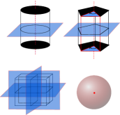
Symmetries are a severe issue when relying on fixed representations of 3D orientations since they cause pose ambiguities (Fig. 2). If not manually addressed, identical training images can have different orientation labels assigned which can significantly disturb the learning process. In order to cope with ambiguous objects, most approaches in literature are manually adapted (Wohlhart and Lepetit, 2015; Hinterstoisser et al., 2012a; Kehl et al., 2017; Rad and Lepetit, 2017). The strategies reach from ignoring one axis of rotation (Wohlhart and Lepetit, 2015; Hinterstoisser et al., 2012a) over adapting the discretization according to the object (Kehl et al., 2017) to the training of an extra CNN to predict symmetries (Rad and Lepetit, 2017). These depict tedious, manual ways to filter out object symmetries (Fig. 2a) in advance, but treating ambiguities due to self-occlusions (Fig. 2b) and occlusions (Fig. 2c) are harder to address.

Symmetries do not only affect regression and classification methods, but any learning-based algorithm that discriminates object views solely by fixed SO(3) representations.

(a) Object symmetries

(b) Self-occlusion induced symmetries

(c) Occlusion induced symmetries

Figure 2: Causes of pose ambiguities

2.3 Learning Representations of 3D orientations

We can also learn indirect pose representations that relate object views in a low-dimensional space. The descriptor learning can either be self-supervised by the object views themselves or still rely on fixed SO(3) representations.

Figure 3: *

(a) $X_{s=1.0,t_{xy}=0.0,r\in[0,2\pi]}$ (b) $X_{s=0.6,t_{xy}=0.0,r\in[0,2\pi]}$ (c) $X_{s=1.0,t_{xy}\sim\mathcal{U}(-1,1),r\in[0,2\pi]}$ (d) $X_{s\sim\mathcal{U}(0.5,1),t_{xy}\sim\mathcal{U}(-1,1),r\in[0,2\pi]}$

Figure 4: *

Figure 5: *

Figure 6: *

Figure 7: *

(1) Autoencoder $\hbox{\pagecolor{darkgreen}(a)}\longrightarrow\hbox{\pagecolor{darkgreen}(a)}$ (2) Autoencoder $\hbox{\pagecolor{darkyellow}(d)}\longrightarrow\hbox{\pagecolor{darkyellow}(d)}$ (3) Augmented Autoencoder $\hbox{\pagecolor{darkyellow}(d)}\longrightarrow\hbox{\pagecolor{darkgreen}(a)}$

Figure 8: *

Figure 9: *

Figure 10: Experiment on the dsprites dataset of Matthey et al. (2017). Left: 64x64 squares from four distributions (a,b,c and d) distinguished by scale ($s$) and translation ($t_{xy}$) that are used for training and testing. Right: Normalized latent dimensions $z_{1}$ and $z_{2}$ for all rotations ($r$) of the distribution (a), (b) or (c) after training ordinary AEs (1),(2) and an AAE (3) to reconstruct squares of the same orientation.

2.3.1 Descriptor Learning

Wohlhart and Lepetit (2015) introduced a CNN-based descriptor learning approach using a triplet loss that minimizes/maximizes the Euclidean distance between similar/dissimilar object orientations. In addition, the distance between different objects is maximized. Although mixing in synthetic data, the training also relies on pose-annotated sensor data. The approach is not immune against symmetries since the descriptor is built using explicit 3D orientations. Thus, the loss can be dominated by symmetric object views that appear the same but have opposite orientations which can produce incorrect average pose predictions.

Balntas et al. (2017) extended this work by enforcing proportionality between descriptor and pose distances. They acknowledge the problem of object symmetries by weighting the pose distance loss with the depth difference of the object at the considered poses. This heuristic increases the accuracy on symmetric objects with respect to Wohlhart and Lepetit (2015).

Our work is also based on learning descriptors, but in contrast we train our Augmented Autoencoders (AAEs) such that the learning process itself is independent of any fixed SO(3) representation. The loss is solely based on the appearance of the reconstructed object views and thus symmetrical ambiguities are inherently regarded. Thus, unlike Balntas et al. (2017); Wohlhart and Lepetit (2015) we abstain from the use of real labeled data during training and instead train completely self-supervised. This means that assigning 3D orientations to the descriptors only happens after the training.

Kehl et al. (2016) train an Autoencoder architecture on random RGB-D scene patches from the LineMOD dataset Hinterstoisser et al. (2011). At test time, descriptors from scene and object patches are compared to find the 6D pose. Since the approach requires the evaluation of a lot of patches, it takes about 670ms per prediction. Furthermore, using local patches means to ignore holistic relations between object features which is crucial if few texture exists. Instead we train on holistic object views and explicitly learn domain invariance.

3 Method

In the following, we mainly focus on the novel 3D orientation estimation technique based on the AAE.

Figure 11: Training process for the AAE; a) reconstruction target batch $\boldsymbol{x}$ of uniformly sampled SO(3) object views; b) geometric and color augmented input; c) reconstruction $\boldsymbol{\hat{x}}$ after 40000 iterations

3.1 Autoencoders

The original AE, introduced by Rumelhart et al. (1985), is a dimensionality reduction technique for high dimensional data such as images, audio or depth. It consists of an Encoder $\Phi$ and a Decoder $\Psi$, both arbitrary learnable function approximators which are usually neural networks. The training objective is to reconstruct the input $x\in\mathcal{R}^{\mathcal{D}}$ after passing through a low-dimensional bottleneck, referred to as the latent representation $z\in\mathcal{R}^{n}$ with $n<<\mathcal{D}$ :

$$\hat{x}=(\Psi\circ\Phi)(x)=\Psi(z)$$ (1)

The per-sample loss is simply a sum over the pixel-wise L2 distance

$$\ell_{2}=\sum_{i\in\mathcal{D}}\parallel x_{i}-\hat{x}_{i}\parallel_{2}$$ (2)

The resulting latent space can, for example, be used for unsupervised clustering.

Denoising Autoencoders introduced by Vincent et al. (2010) have a modified training procedure. Here, artificial random noise is applied to the input images $x\in\mathcal{R}^{\mathcal{D}}$ while the reconstruction target stays clean. The trained model can be used to reconstruct denoised test images. But how is the latent representation affected?

Hypothesis 1: The Denoising AE produces latent representations which are invariant to noise because it facilitates the reconstruction of de-noised images.

We will demonstrate that this training strategy actually enforces invariance not only against noise but against a variety of different input augmentations. Finally, it allows us to bridge the domain gap between simulated and real data.

3.2 Augmented Autoencoder

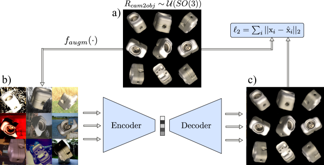
The motivation behind the AAE is to control what the latent representation encodes and which properties are ignored. We apply random augmentations $f_{augm}(.)$ to the input images $x\in\mathcal{R}^{\mathcal{D}}$ against which the encoding should become invariant. The reconstruction target remains eq. (2) but eq. (1) becomes

$$\hat{x}=(\Psi\circ\Phi\circ f_{augm})(x)=(\Psi\circ\Phi)(x^{\prime})=\Psi(z^{\prime})$$ (3)

To make evident that Hypothesis 1 holds for geometric transformations, we learn latent representations of binary images depicting a 2D square at different scales, in-plane translations and rotations. Our goal is to encode only the in-plane rotations $r\in[0,2\pi]$ in a two dimensional latent space $z\in\mathcal{R}^{2}$ independent of scale or translation. Fig. 10 depicts the results after training a CNN-based AE architecture similar to the model in Fig. 12. It can be observed that the AEs trained on reconstructing squares at fixed scale and translation (1) or random scale and translation (2) do not clearly encode rotation alone, but are also sensitive to other latent factors. Instead, the encoding of the AAE (3) becomes invariant to translation and scale such that all squares with coinciding orientation are mapped to the same code. Furthermore, the latent representation is much smoother and the latent dimensions imitate a shifted sine and cosine function with frequency $f=\frac{4}{2\pi}$ respectively. The reason is that the square has two perpendicular axes of symmetry, i.e. after rotating $\frac{\pi}{2}$ the square appears the same. This property of representing the orientation based on the appearance of an object rather than on a fixed parametrization is valuable to avoid ambiguities due to symmetries when teaching 3D object orientations.

Figure 12: Autoencoder CNN architecture with occluded test input, ”resize2x” depicts nearest-neighbor upsampling

3.3 Learning 3D Orientation from Synthetic Object Views

Our toy problem showed that we can explicitly learn representations of object in-plane rotations using a geometric augmentation technique. Applying the same geometric input augmentations we can encode the whole SO(3) space of views from a 3D object model (CAD or 3D reconstruction) while being robust against inaccurate object detections. However, the encoder would still be unable to relate image crops from real RGB sensors because (1) the 3D model and the real object differ, (2) simulated and real lighting conditions differ, (3) the network can’t distinguish the object from background clutter and foreground occlusions. Instead of trying to imitate every detail of specific real sensor recordings in simulation we propose a Domain Randomization (DR) technique within the AAE framework to make the encodings invariant to insignificant environment and sensor variations. The goal is that the trained encoder treats the differences to real camera images as just another irrelevant variation. Therefore, while keeping reconstruction targets clean, we randomly apply additional augmentations to the input training views: (1) rendering with random light positions and randomized diffuse and specular reflection (simple Phong model (Phong, 1975) in OpenGL), (2) inserting random background images from the Pascal VOC dataset (Everingham et al., 2012), (3) varying image contrast, brightness, Gaussian blur and color distortions, (4) applying occlusions using random object masks or black squares. Fig. 11 depicts an exemplary training process for synthetic views of object 5 from T-LESS (Hodaň et al., 2017).

Table 1: Augmentation Parameters of AAE; Scale and translation is in relation to image shape and occlusion is in proportion of the object mask

	50% chance	light (random position)
	(30% per channel)	& geometric
add	$\mathcal{U}(-0.1,0.1)$	ambient	$0.4$
contrast	$\mathcal{U}(0.4,2.3)$	diffuse	$\mathcal{U}(0.7,0.9)$
multiply	$\mathcal{U}(0.6,1.4)$	specular	$\mathcal{U}(0.2,0.4)$
invert		scale	$\mathcal{U}(0.8,1.2)$
gaussian blur	$\sigma\sim\mathcal{U}(0.0,1.2)$	translation	$\mathcal{U}(-0.15,0.15)$
		occlusion	$\in[0,0.25]$

Figure 13: AAE decoder reconstruction of LineMOD (left) and T-LESS (right) scene crops

3.4 Network Architecture and Training Details

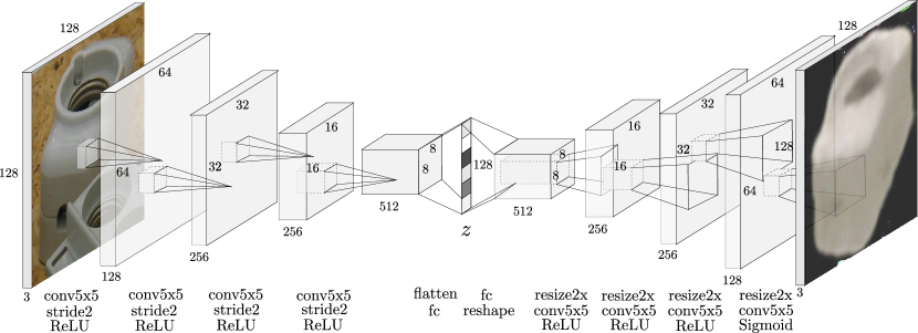
The convolutional Autoencoder architecture that is used in our experiments is depicted in Fig. 12. We use a bootstrapped pixel-wise L2 loss, first introduced by Wu et al. (2016). Only the pixels with the largest reconstruction errors contribute to the loss. Thereby, finer details are reconstructed and the training does not converge to local minima like reconstructing black images for all views. In our experiments, we choose a bootstrap factor of $k=4$ per image, meaning that $\frac{1}{4}$ of all pixels contribute to the loss. Using OpenGL, we render 20000 views of each object uniformly at random 3D orientations and constant distance along the camera axis (700mm). The resulting images are quadratically cropped using the longer side of the bounding box and resized (nearest neighbor) to $128\times 128\times 3$ as shown in Fig. 11. All geometric and color input augmentations besides the rendering with random lighting are applied online during training at uniform random strength, parameters are found in Tab. 1. We use the Adam (Kingma and Ba, 2014) optimizer with a learning rate of $2\times 10^{-4}$, Xavier initialization (Glorot and Bengio, 2010), a batch size = 64 and 40000 iterations which takes $\sim 4$ hours on a single Nvidia Geforce GTX 1080.

Figure 14: Top: creating a codebook from the encodings of discrete synthetic object views; bottom: object detection and 3D orientation estimation using the nearest neighbor(s) with highest cosine similarity from the codebook

3.5 Codebook Creation and Test Procedure

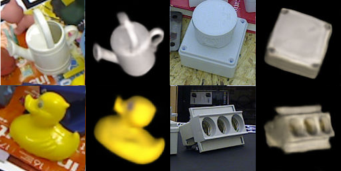
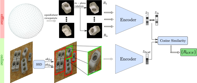
After training, the AAE is able to extract a 3D object from real scene crops of many different camera sensors (Fig. 13). The clarity and orientation of the decoder reconstruction is an indicator of the encoding quality. To determine 3D object orientations from test scene crops we create a codebook (Fig. 14 (top)):

• Render clean, synthetic object views at nearly equidistant viewpoints from a full view-sphere (based on a refined icosahedron (Hinterstoisser et al., 2008))

• Rotate each view in-plane at fixed intervals to cover the whole SO(3)

• Create a codebook by generating latent codes $z\in\mathcal{R}^{128}$ for all resulting images and assigning their corresponding rotation $R_{cam2obj}\in\mathcal{R}^{3x3}$

At test time, the considered object(s) are first detected in an RGB scene. The image is quadratically cropped using the longer side of the bounding box multiplied with a padding factor of 1.2 and resized to match the encoder input size. The padding accounts for imprecise bounding boxes. After encoding we compute the cosine similarity between the test code $z_{test}\in\mathcal{R}^{128}$ and all codes $z_{i}\in\mathcal{R}^{128}$ from the codebook:

$$cos_{i}=\frac{\boldsymbol{z}_{i}\;\boldsymbol{z}_{test}}{\lVert\boldsymbol{z}_{i}\rVert\lVert\boldsymbol{z}_{test}\rVert}$$ (4)

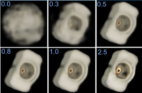
The highest similarities are determined in a k-Nearest-Neighbor (kNN) search and the corresponding rotation matrices $\{R_{kNN}\}$ from the codebook are returned as estimates of the 3D object orientation. For the quantitative evaluation we use $k=1$, however the next neighbors can yield valuable information on ambiguous views and could for example be used in particle filter based tracking. We use cosine similarity because (1) it can be very efficiently computed on a single GPU even for large codebooks. In our experiments we have 2562 equidistant viewpoints $\times$ 36 in-plane rotation = 92232 total entries. (2) We observed that, presumably due to the circular nature of rotations, scaling a latent test code does not change the object orientation of the decoder reconstruction (Fig. 15).

Figure 15: AAE decoder reconstruction of a test code $z_{test}\in\mathcal{R}^{128}$ scaled by a factor $s\in[0,2.5]$

Table 2: Augmentation Parameters for Object Detectors, top five are applied in random order; bottom part describes phong lighting from random light positions

	chance	SIXD train	Rendered
	(per ch.)		3D models
add	0.5 (0.15)	$\mathcal{U}(-0.08,0.08)$	$\mathcal{U}(-0.1,0.1)$
contrast norm.	0.5 (0.15)	$\mathcal{U}(0.5,2.2)$	$\mathcal{U}(0.5,2.2)$
multiply	0.5 (0.25)	$\mathcal{U}(0.6,1.4)$	$\mathcal{U}(0.5,1.5)$
gaussian blur	0.2	$\sigma\sim\mathcal{U}(0.5,1.0)$	$\sigma=0.4$
gaussian noise	0.1 (0.1)	$\sigma=0.04$	-
ambient	1.0	-	$0.4$
diffuse	1.0	-	$\mathcal{U}(0.7,0.9)$
specular	1.0	-	$\mathcal{U}(0.2,0.4)$

3.6 Extending to 6D Object Detection

3.6.1 Training the 2D Object Detector.

We finetune the 2D Object Detectors using the object views on black background which are provided in the training datasets of LineMOD and T-LESS. In LineMOD we additionally render domain randomized views of the provided 3D models and freeze the backbone like in Hinterstoisser et al. (2017). Multiple object views are sequentially copied into an empty scene at random translation, scale and in-plane rotation. Bounding box annotations are adapted accordingly. If an object view is more than 40% occluded, we re-sample it. Then, as for the AAE, the black background is replaced with Pascal VOC images. The randomization schemes and parameters can be found in Table 2. In T-LESS we train SSD (Liu et al., 2016) with VGG16 backbone and RetinaNet (Lin et al., 2018) with ResNet50 backbone which is slower but more accurate, on LineMOD we only train RetinaNet. For T-LESS we generate 60000 training samples from the provided training dataset and for LineMOD we generate 60000 samples from the training dataset plus 60000 samples from 3D model renderings with randomized lighting conditions (see Table 2). The RetinaNet achieves 0.73mAP@0.5IoU on T-LESS and 0.62mAP@0.5IoU on LineMOD. On Occluded LineMOD, the detectors trained on the simplistic renderings failed to achieve good detection performance. However, recent work of Hodan et al. (2019) quantitatively investigated the training of 2D detectors on synthetic data and they reached decent detection performance on Occluded LineMOD by fine-tuning FasterRCNN on photo-realistic synthetic images showing the feasibility of a purely synthetic pipeline.

3.6.2 Projective Distance Estimation

We estimate the full 3D translation $t_{real}$ from camera to object center, similar to Kehl et al. (2017). Therefore, we save the 2D bounding box for each synthetic object view in the codebook and compute its diagonal length $\|bb_{syn,i}\|$. At test time, we compute the ratio between the detected bounding box diagonal $\|bb_{real}\|$ and the corresponding codebook diagonal $\|bb_{syn,{\operatorname*{argmax}}(cos_{i})}\|$, i.e. at similar orientation. The pinhole camera model yields the distance estimate $\hat{t}_{real,z}$

$$\hat{t}_{real,z}=t_{syn,z}\times\frac{\|bb_{syn,{\operatorname*{argmax}}(cos_{i})}\|}{\|bb_{real}\|}\times\frac{f_{real}}{f_{syn}}$$ (5)

with synthetic rendering distance $t_{syn,z}$ and focal lengths $f_{real}$, $f_{syn}$ of the real sensor and synthetic views. It follows that

$$\boldsymbol{\Delta\hat{t}} =\hat{t}_{real,z}\boldsymbol{K_{real}^{-1}}\boldsymbol{bb_{real,c}}-t_{syn,z}\boldsymbol{K_{syn}^{-1}}\boldsymbol{bb_{syn,c}}$$ (6)

$$\boldsymbol{\hat{t}_{real}} =\boldsymbol{t_{syn}}+\boldsymbol{\Delta\hat{t}}$$ (7)

where $\boldsymbol{\Delta\hat{t}}$ is the estimated vector from the synthetic to the real object center, $\boldsymbol{K_{real}},\boldsymbol{K_{syn}}$ are the camera matrices, $\boldsymbol{bb_{real,c}},\boldsymbol{bb_{syn,c}}$ are the bounding box centers in homogeneous coordinates and $\boldsymbol{\hat{t}_{real}},\boldsymbol{t_{syn}}=(0,0,t_{syn,z})$ are the translation vectors from camera to object centers. In contrast to Kehl et al. (2017), we can predict the 3D translation for different test intrinsics.

3.6.3 Perspective Correction

While the codebook is created by encoding centered object views, the test image crops typically do not originate from the image center. Naturally, the appearance of the object view changes when translating the object in the image plane at constant object orientation. This causes a noticeable error in the rotation estimate from the codebook towards the image borders. However, this error can be corrected by determining the object rotation that approximately preserves the appearance of the object when translating it to our estimate $\boldsymbol{\hat{t}_{real}}$.

$$\left(\begin{array}[]{c}\alpha_{x}\\ \alpha_{y}\end{array}\right) =\left(\begin{array}[]{c}-\arctan(\hat{t}_{real,y}/\hat{t}_{real,z})\\ \arctan(\hat{t}_{real,x}/\sqrt{\hat{t}_{real,z}^{2}+\hat{t}^{2}_{real,y}})\end{array}\right)$$ (12)

$$\boldsymbol{\hat{R}_{obj2cam}} =\boldsymbol{R_{y}(}\alpha_{y}\boldsymbol{)R_{x}(}\alpha_{x}\boldsymbol{)\hat{R}^{\prime}_{obj2cam}}$$ (13)

where $\alpha_{x},\alpha_{y}$ describe the angles around the camera axes and $\boldsymbol{R_{y}(}\alpha_{y}\boldsymbol{)R_{x}(}\alpha_{x}\boldsymbol{)}$ the corresponding rotation matrices to correct the initial rotation estimate $\boldsymbol{\hat{R}^{\prime}_{obj2cam}}$ from object to camera. The perspective corrections give a notable boost in accuracy as reported in Table 7. If strong perspective distortions are expected at test time, the training images $x^{\prime}$ could also be recorded at random distances as opposed to constant distance. However, in the benchmarks, perspective distortions are minimal and consequently random online image-plane scaling of $x^{\prime}$ is sufficient.

3.6.4 ICP Refinement

Optionally, the estimate is refined on depth data using a point-to-plane ICP approach with adaptive thresholding of correspondences based on Chen and Medioni (1992); Zhang (1994) taking an average of $\sim 320ms$. The refinement is first applied in direction of the vector pointing from camera to the object where most of the RGB-based pose estimation errors stem from and then on the full 6D pose.

3.6.5 Inference Time

The Single Shot Multibox Detector (SSD) with VGG16 base and 31 classes plus the AAE (Fig. 12) with a codebook size of $92232\times 128$ yield the average inference times depicted in Table 3. We conclude that the RGB-based pipeline is real-time capable at $\sim$42Hz on a Nvidia GTX 1080. This enables augmented reality and robotic applications and leaves room for tracking algorithms. Multiple encoders (15MB) and corresponding codebooks (45MB each) fit into the GPU memory, making multi-object pose estimation feasible.

Table 3: Inference time of the RGB pipeline using SSD on CPUs or GPU

	4 CPUs	GPU
SSD	-	$\sim$17ms
Encoder	$\sim$100ms	$\sim$5ms
Cosine Similarity	2.5ms	1.3ms
Nearest Neighbor	0.3ms	3.2ms
Projective Distance	0.4ms	-
	$\sim$24ms

Table 4: Single object pose estimation runtime w/o refinement

Method	fps
Vidal et al. (2018)	$0.2$
Brachmann et al. (2016)	2
Kehl et al. (2016)	2
Rad and Lepetit (2017)	4
Kehl et al. (2017)	12
OURS	13 (RetinaNet)
	42 (SSD)
Tekin et al. (2017)	50

Table 5: Ablation study on color augmentations for different test sensors. Object 5 tested on all scenes, T-LESS Hodaň et al. (2017). Standard deviation of three runs in brackets.

Train RGB Test RGB dyn. light add contrast multiply invert AUC_vsd 3D Reconstruction Primesense ✓ 0.472 ($\pm$ 0.013) (synthetic) (real) ✓ ✓ 0.611 ($\pm$ 0.030) ✓ ✓ ✓ 0.825 ($\pm$ 0.015) ✓ ✓ ✓ ✓ 0.876 ($\pm$ 0.019) ✓ ✓ ✓ ✓ ✓ 0.877 ($\pm$ 0.005) ✓ ✓ ✓ 0.861 ($\pm$ 0.014) Primesense (real) Primesense (real) ✓ ✓ ✓ 0.890 ($\pm$ 0.003) 3D Reconstruction Kinect ✓ 0.461 ($\pm$ 0.022) (synthetic) (real) ✓ ✓ 0.580 ($\pm$ 0.014) ✓ ✓ ✓ 0.701 ($\pm$ 0.046) ✓ ✓ ✓ ✓ 0.855 ($\pm$ 0.016) ✓ ✓ ✓ ✓ ✓ 0.897 ($\pm$ 0.008) ✓ ✓ ✓ 0.903 ($\pm$ 0.016) Kinect (real) Kinect (real) ✓ ✓ ✓ 0.917 ($\pm$ 0.007)

(a) Effect of latent space size, standard deviation in red

(b) Training on CAD model (bottom) vs. textured 3D reconstruction (top)

Figure 16: Testing object 5 on all 504 Kinect RGB views of scene 2 in T-LESS

4 Evaluation

We evaluate the AAE and the whole 6D detection pipeline on the T-LESS (Hodaň et al., 2017) and LineMOD (Hinterstoisser et al., 2011) datasets.

4.1 Test Conditions

Few RGB-based pose estimation approaches (e.g. Kehl et al. (2017); Ulrich et al. (2009)) only rely on 3D model information. Most methods like Wohlhart and Lepetit (2015); Balntas et al. (2017); Brachmann et al. (2016) make use of real pose annotated data and often even train and test on the same scenes (e.g. at slightly different viewpoints, as in the official LineMOD benchmark). It is common practice to ignore in-plane rotations or to only consider object poses that appear in the dataset (Rad and Lepetit, 2017; Wohlhart and Lepetit, 2015) which also limits applicability. Symmetric object views are often individually treated (Rad and Lepetit, 2017; Balntas et al., 2017) or ignored (Wohlhart and Lepetit, 2015). The SIXD challenge (Hodan, 2017) is an attempt to make fair comparisons between 6D localization algorithms by prohibiting the use of test scene pixels. We follow these strict evaluation guidelines, but treat the harder problem of 6D detection where it is unknown which of the considered objects are present in the scene. This is especially difficult in the T-LESS dataset since objects are very similar. We train the AAEs on the reconstructed 3D models, except for object 19-23 where we train on the CAD models because the pins are missing in the reconstructed plugs.

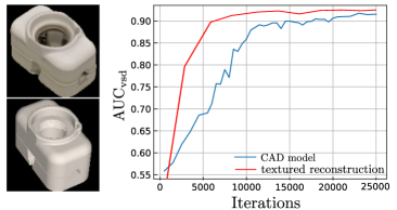
We noticed, that the geometry of some 3D reconstruction in T-LESS is slightly inaccurate which badly influences the RGB-based distance estimation (Sec. 3.6.2) since the synthetic bounding box diagonals are wrong. Therefore, in a second training run we only train on the 30 CAD models.

Table 6: T-LESS: Object recall for $err_{vsd}<0.3$ on all Primesense test scenes (SIXD/BOP benchmark from Hodan et al. (2018)). $RGB^{\dagger}$ depicts training with 3D reconstructions, except objects 19-23 $\longrightarrow$ CAD models; $RGB^{\ddagger}$ depicts training on untextured CAD models only

AAE AAE AAE SSD RetinaNet RetinaNet Brachmann et al. Kehl et al. Vidal et al. Drost et al. w/ GT 2D BBs Data $RGB^{\dagger}$ $RGB^{\dagger}$ $RGB^{\ddagger}$ $RGB^{\dagger}$+Depth(ICP) RGB-D RGB-D +ICP Depth +ICP Depth +edge $RGB^{\dagger}$ +Depth(ICP) 1 5.65 9.48 12.67 67.95 8 7 43 53 12.67 85.98 2 5.46 13.24 16.01 70.62 10 10 47 44 11.47 86.27 3 7.05 12.78 22.84 78.39 21 18 69 61 13.32 90.80 4 4.61 6.66 6.70 57.00 4 24 63 67 12.88 84.20 5 36.45 36.19 38.93 77.18 46 23 69 71 67.37 90.14 6 23.15 20.64 28.26 72.75 19 10 67 73 54.21 90.58 7 15.97 17.41 26.56 83.39 52 0 77 75 38.10 86.94 8 10.86 21.72 18.01 78.08 22 2 79 89 24.83 91.79 9 19.59 39.98 33.36 88.64 12 11 90 92 49.06 91.09 10 10.47 13.37 33.15 84.47 7 17 68 72 15.67 84.67 11 4.35 7.78 17.94 56.01 3 5 69 64 16.64 77.01 12 7.80 9.54 18.38 63.23 3 1 82 81 33.57 79.32 13 3.30 4.56 16.20 43.55 0 0 56 53 15.29 64.38 14 2.85 5.36 10.58 25.58 0 9 47 46 50.14 71.37 15 7.90 27.11 40.50 69.81 0 12 52 55 52.01 73.90 16 13.06 22.04 35.67 84.55 5 56 81 85 36.71 87.58 17 41.70 66.33 50.47 74.29 3 52 83 88 81.44 78.88 18 47.17 14.91 33.63 83.12 54 22 80 78 55.48 85.64 19 15.95 23.03 23.03 58.13 38 35 55 55 53.07 82.71 20 2.17 5.35 5.35 26.73 1 5 47 47 38.97 70.87 21 19.77 19.82 19.82 53.48 39 26 63 55 53.45 86.83 22 11.01 20.25 20.25 60.49 19 27 70 56 49.95 84.20 23 7.98 19.15 19.15 62.69 61 71 85 84 36.74 76.40 24 4.74 4.54 27.94 62.99 1 36 70 59 11.75 84.38 25 21.91 19.07 51.01 73.33 16 28 48 47 37.73 87.53 26 10.04 12.92 33.00 67.00 27 51 55 69 29.82 90.26 27 7.42 22.37 33.61 82.16 17 34 60 61 23.30 84.43 28 21.78 24.00 30.88 83.51 13 54 69 80 43.97 89.84 29 15.33 27.66 35.57 74.45 6 86 65 84 57.82 88.58 30 34.63 30.53 44.33 93.65 5 69 84 89 72.81 95.01 Mean 14.67 19.26 26.79 68.57 17.84 24.60 66.51 67.50 38.34 84.05 Time(s) 0.024 0.077 0.077 0.4 13.5 1.8 4.7 21.5 0.006 0.33

Table 7: Effect of Perspective Corrections on T-LESS

Method	$RGB^{\dagger}$
w/o correction	18.35
w/ correction	19.26 (+0.91)

4.2 Metrics

Hodaň et al. (2016) introduced the Visible Surface Discrepancy ($err_{vsd}$), an ambiguity-invariant pose error function that is determined by the distance between the estimated and ground truth visible object depth surfaces. As in the SIXD challenge, we report the recall of correct 6D object poses at $err_{vsd}<0.3$ with tolerance $\tau=20mm$ and $>10\%$ object visibility. Although the Average Distance of Model Points (ADD) metric introduced by Hinterstoisser et al. (2012b) cannot handle pose ambiguities, we also present it for the LineMOD dataset following the official protocol in Hinterstoisser et al. (2012b). For objects with symmetric views (eggbox, glue), Hinterstoisser et al. (2012b) adapts the metric by calculating the average distance to the closest model point. Manhardt et al. (2018) has noticed inaccurate intrinsics and sensor registration errors between RGB and D in the LineMOD dataset. Thus, purely synthetic RGB-based approaches, although visually correct, suffer from false pose rejections. The focus of our experiments lies on the T-LESS dataset.

In our ablation studies we also report the $AUC_{vsd}$, which represents the area under the ’$err_{vsd}$ vs. recall’ curve:

$$AUC_{vsd}=\int_{0}^{1}recall(err_{vsd})\,derr_{vsd}$$ (14)

4.3 Ablation Studies

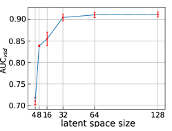
To assess the AAE alone, in this subsection we only predict the 3D orientation of Object 5 from the T-LESS dataset on Primesense and Kinect RGB scene crops. Table 5 shows the influence of different input augmentations. It can be seen that the effect of different color augmentations is cumulative. For textureless objects, even the inversion of color channels seems to be beneficial since it prevents overfitting to synthetic color information. Furthermore, training with real object recordings provided in T-LESS with random Pascal VOC background and augmentations yields only slightly better performance than the training with synthetic data. Fig. 16a depicts the effect of different latent space sizes on the 3D pose estimation accuracy. Performance starts to saturate at $dim=64$.

Table 8: LineMOD: Object recall (ADD Hinterstoisser et al. (2012b) metric) of methods that use different amounts of training and test data, results taken from Tekin et al. (2017)

Test data RGB       +Depth (ICP) Train data RGB w/o real pose labels RGB with real pose labels – Object Kehl et al. OURS Brachmann et al. Rad and Lepetit Tekin et al. Xiang et al. OURS Kehl et al. +refine +refine +DeepIm Ape 0.00 4.18 - 33.2 27.9 40.4 21.62 - 77.0 24.35 65 Benchvise 0.18 22.85 - 64.8 62.0 91.8 81.80 - 97.5 89.13 80 Cam 0.41 32.91 - 38.4 40.1 55.7 36.57 - 93.5 82.10 78 Can 1.35 37.03 - 62.9 48.1 64.1 68.80 - 96.5 70.82 86 Cat 0.51 18.68 - 42.7 45.2 62.6 41.82 - 82.1 72.18 70 Driller 2.58 24.81 - 61.9 58.6 74.4 63.51 - 95.0 44.87 73 Duck 0.00 5.86 - 30.2 32.8 44.3 27.23 - 77.7 54.63 66 Eggbox 8.90 81.00 - 49.9 40.0 57.8 69.58 - 97.1 96.62 100 Glue 0.00 46.17 - 31.2 27.0 41.2 80.02 - 99.4 94.18 100 Holepuncher 0.30 18.20 - 52.8 42.4 67.2 42.63 - 52.8 51.25 49 Iron 8.86 35.05 - 80.0 67.0 84.7 74.97 - 98.3 77.86 78 Lamp 8.2 61.15 - 67.0 39.9 76.5 71.11 - 97.5 86.31 73 Phone 0.18 36.27 - 38.1 35.2 54.0 47.74 - 87.7 86.24 79 Mean 2.42 32.63 32.3 50.2 43.6 62.7 55.95 62.7 88.6 71.58 79

(a) Object 5, one view-dependent symmetry

(b) Object 28, two view-dependent symmetries

Figure 17: Rotation and translation error histograms on all T-LESS test scenes with our RGB-based (left columns) and ICP-refined (right columns) 6D Object Detection

(a)

(b)

(c)

Figure 18: Failure cases; Blue: True poses; Green: Predictions; (a) Failed detections due to occlusions and object ambiguity, (b) failed AAE predictions of Glue (middle) and Eggbox (right) due to strong occlusion, (c) inaccurate predictions due to occlusion

4.4 Discussion of 6D Object Detection results

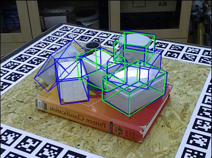
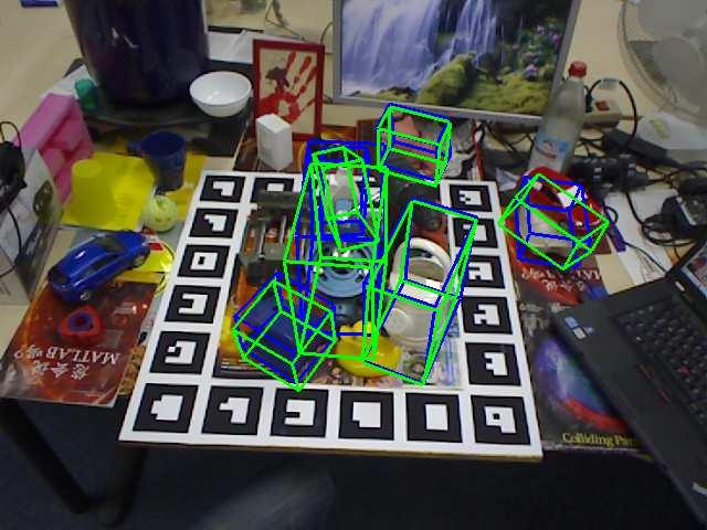
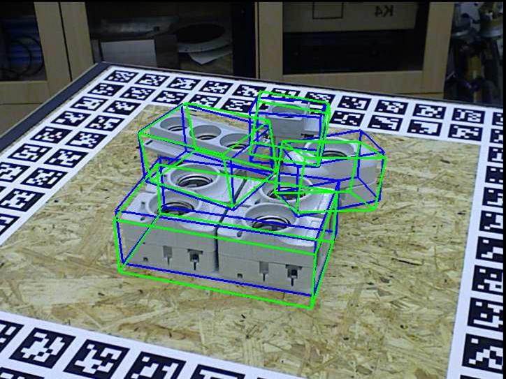
Our RGB-only 6D Object Detection pipeline consists of 2D detection, 3D orientation estimation, projective distance estimation and perspective error correction. Although the results are visually appealing, to reach the performance of state-of-the-art depth-based methods we also need to refine our estimates using a depth-based ICP. Table 6 presents our 6D detection evaluation on all scenes of the T-LESS dataset, which contains a high amount of pose ambiguities. Our pipeline outperforms all 15 reported T-LESS results on the 2018 BOP benchmark from Hodan et al. (2018) in a fraction of the runtime. Table 6 shows an extract of competing methods. Our RGB-only results can compete with the RGB-D learning-based approaches of Brachmann et al. (2016) and Kehl et al. (2016). Previous state-of-the-art approaches from Vidal et al. (2018); Drost et al. (2010) perform a time consuming refinement search through multiple pose hypotheses while we only perform the ICP on a single pose hypothesis. That being said, the codebook is well suited to generate multiple hypotheses using $k>1$ nearest neighbors. The right part of Table 6 shows results with ground truth bounding boxes yielding an upper bound on the pose estimation performance.

The results in Table 6 show that our domain randomization strategy allows to generalize from 3D reconstructions as well as untextured CAD models as long as the considered objects are not significantly textured. Instead of a performance drop we report an increased $err_{vsd}$ $<0.3$ recall due to the more accurate geometry of the model which results in correct bounding box diagonals and thus a better projective distance estimation in the RGB-domain.

In Table 8 we also compare our pipeline against state-of-the-art methods on the LineMOD dataset. Here, our synthetically trained pipeline does not reach the performance of approaches that use real pose annotated training data.

There are multiple issues: (1) As described in Sec 4.1 the real training and test set are strongly correlated and approaches using the real training set can over-fit to it; (2) the models provided in LineMOD are quite bad which affects both, the detection and pose estimation performance of synthetically trained approaches; (3) the advantage of not suffering from pose-ambiguities does not matter much in LineMOD where most object views are pose-ambiguity free; (4) We train and test poses from the whole SO(3) as opposed to only a limited range in which the test poses lie. SSD6D also trains only on synthetic views of the 3D models and we outperform their approach by a big margin in the RGB-only domain before ICP refinement.

4.5 Failure Cases

Figure 18 shows qualitative failure cases, mostly stemming from missed detections and strong occlusions. A weak point is the dependence on the bounding box size at test time to predict the object distance. Specifically, under sever occlusions the predicted bounding box tends to shrink such that it does not encompass the occluded parts of the detected object even if it is trained to do so. If the usage of depth data is clear in advance other methods for directly using depth-based methods for distance estimation might be better suited. Furthermore, on strongly textured objects, the AAEs should not be trained without rendering the texture since otherwise the texture might not be distinguishable from shape at test time. The sim2real transfer on strongly reflective objects like satellites can be challenging and might require physically-based renderings. Some objects, like long, thin pens can fail because their tight object crops at training and test time appear very near from some views and very far from other views, thus hindering the learning of proper pose representations. As the object size is unknown during test time, we cannot simply crop a constantly sized area.

Figure 19: MobileNetSSD and AAEs on T-LESS objects, demonstrated live at ECCV 2018 on a Jetson TX2

4.6 Rotation and Translation Histograms

To investigate the effect of ICP and to obtain an intuition about the pose errors, we plot the rotation and translation error histograms of two T-LESS objects (Fig. 17). We can see the view-dependent symmetry axes of both objects in the rotation errors histograms. We also observe that the translation error is strongly improved through the depth-based ICP while the rotation estimates from the AAE are hardly refined. Especially when objects are partly occluded, the bounding boxes can become inaccurate and the projective distance estimation (Sec. 3.6.2) fails to produce very accurate distance predictions. Still, our global and fast 6D Object Detection provides sufficient accuracy for an iterative local refinement method to reliably converge.

4.7 Demonstration on Embedded Hardware

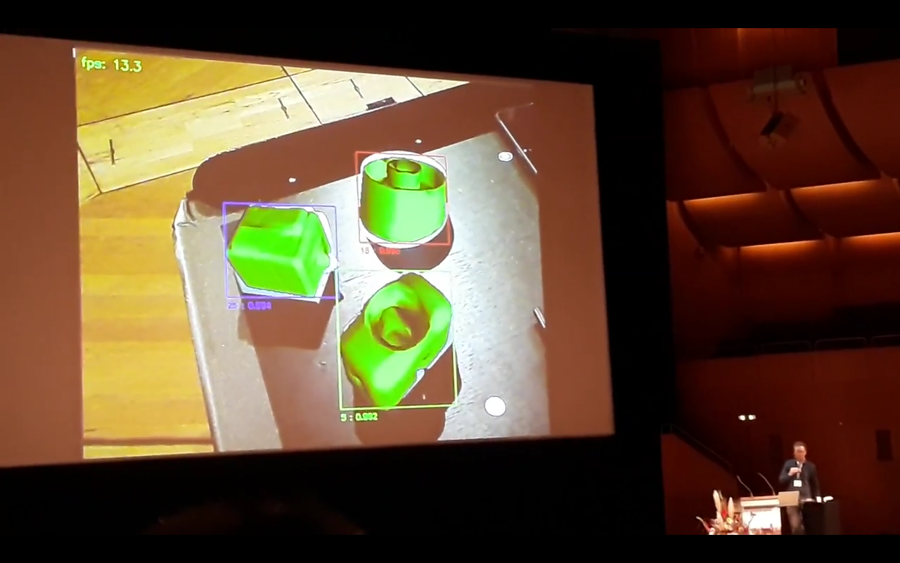
The presented AAEs were also ported onto a Nvidia Jetson TX2 board, together with a small footprint MobileNet from Howard et al. (2017) for the bounding box detection. A webcam was connected, and this setup was demonstrated live at ECCV 2018, both in the demo session and during the oral presentation. For this demo we acquired several of the T-LESS objects. As can be seen in Figure 19, lighting conditions were dramatically different than in the test sequences from the T-LESS dataset which validates the robustness and applicability of our approach outside lab conditions. No ICP was used, so the errors in depth resulting from the scaling errors of the MobileNet, were not corrected. However, since small errors along the depth direction are less perceptible for humans, our approach could be interesting for augmented reality applications. The detection, pose estimation and visualization of the three test objects ran at over 13Hz.

5 Conclusion

We have proposed a new self-supervised training strategy for Autoencoder architectures that enables robust 3D object orientation estimation on various RGB sensors while training only on synthetic views of a 3D model. By demanding the Autoencoder to revert geometric and color input augmentations, we learn representations that (1) specifically encode 3D object orientations, (2) are invariant to a significant domain gap between synthetic and real RGB images, (3) inherently regard pose ambiguities from symmetric object views. Around this approach, we created a real-time (42 fps), RGB-based pipeline for 6D object detection which is especially suitable when pose-annotated RGB sensor data is not available.

References

- Balntas et al. (2017) Balntas V, Doumanoglou A, Sahin C, Sock J, Kouskouridas R, Kim TK (2017) Pose Guided RGB-D Feature Learning for 3D Object Pose Estimation. In: Proceedings of the IEEE Conference on Computer Vision and Pattern Recognition, pp 3856–3864
- Bousmalis et al. (2017a) Bousmalis K, Irpan A, Wohlhart P, Bai Y, Kelcey M, Kalakrishnan M, Downs L, Ibarz J, Pastor P, Konolige K, et al. (2017a) Using simulation and domain adaptation to improve efficiency of deep robotic grasping. arXiv preprint arXiv:170907857
- Bousmalis et al. (2017b) Bousmalis K, Silberman N, Dohan D, Erhan D, Krishnan D (2017b) Unsupervised pixel-level domain adaptation with generative adversarial networks. In: The IEEE Conference on Computer Vision and Pattern Recognition (CVPR), vol 1, p 7
- Brachmann et al. (2016) Brachmann E, Michel F, Krull A, Ying Yang M, Gumhold S, et al. (2016) Uncertainty-driven 6D pose estimation of objects and scenes from a single RGB image. In: Proceedings of the IEEE Conference on Computer Vision and Pattern Recognition, pp 3364–3372
- Chen and Medioni (1992) Chen Y, Medioni G (1992) Object modelling by registration of multiple range images. Image and vision computing 10(3):145–155
- Csurka (2017) Csurka G (2017) Domain adaptation for visual applications: A comprehensive survey. arXiv preprint arXiv:170205374
- Drost et al. (2010) Drost B, Ulrich M, Navab N, Ilic S (2010) Model globally, match locally: Efficient and robust 3d object recognition. In: 2010 IEEE computer society conference on computer vision and pattern recognition, Ieee, pp 998–1005
- Everingham et al. (2012) Everingham M, Van Gool L, Williams CKI, Winn J, Zisserman A (2012) The PASCAL Visual Object Classes Challenge 2012 (VOC2012) Results
- Glorot and Bengio (2010) Glorot X, Bengio Y (2010) Understanding the difficulty of training deep feedforward neural networks. In: Proceedings of the Thirteenth International Conference on Artificial Intelligence and Statistics, pp 249–256
- Hinterstoisser et al. (2008) Hinterstoisser S, Benhimane S, Lepetit V, Fua P, Navab N (2008) Simultaneous Recognition and Homography Extraction of Local Patches with a Simple Linear Classifier. In: Proceedings of the British Machine Conference, pages, pp 10–1
- Hinterstoisser et al. (2011) Hinterstoisser S, Holzer S, Cagniart C, Ilic S, Konolige K, Navab N, Lepetit V (2011) Multimodal templates for real-time detection of texture-less objects in heavily cluttered scenes. In: Computer Vision (ICCV), 2011 IEEE International Conference on, IEEE, pp 858–865
- Hinterstoisser et al. (2012a) Hinterstoisser S, Cagniart C, Ilic S, Sturm P, Navab N, Fua P, Lepetit V (2012a) Gradient response maps for real-time detection of textureless objects. IEEE Transactions on Pattern Analysis and Machine Intelligence 34(5):876–888
- Hinterstoisser et al. (2012b) Hinterstoisser S, Lepetit V, Ilic S, Holzer S, Bradski G, Konolige K, Navab N (2012b) Model based training, detection and pose estimation of texture-less 3D objects in heavily cluttered scenes. In: Asian conference on computer vision, Springer, pp 548–562
- Hinterstoisser et al. (2016) Hinterstoisser S, Lepetit V, Rajkumar N, Konolige K (2016) Going further with Point Pair Features. In: European Conference on Computer Vision, Springer, pp 834–848
- Hinterstoisser et al. (2017) Hinterstoisser S, Lepetit V, Wohlhart P, Konolige K (2017) On Pre-Trained Image Features and Synthetic Images for Deep Learning. arXiv preprint arXiv:171010710
- Hodan (2017) Hodan T (2017) SIXD Challenge 2017, http://cmp.felk.cvut.cz/sixd/challenge˙2017/
- Hodaň et al. (2016) Hodaň T, Matas J, Obdržálek Š (2016) On evaluation of 6D object pose estimation. In: European Conference on Computer Vision, Springer, pp 606–619
- Hodaň et al. (2017) Hodaň T, Haluza P, Obdržálek Š, Matas J, Lourakis M, Zabulis X (2017) T-LESS: An RGB-D Dataset for 6D Pose Estimation of Texture-less Objects. IEEE Winter Conference on Applications of Computer Vision (WACV)
- Hodan et al. (2018) Hodan T, Michel F, Brachmann E, Kehl W, GlentBuch A, Kraft D, Drost B, Vidal J, Ihrke S, Zabulis X, et al. (2018) Bop: benchmark for 6d object pose estimation. In: Proceedings of the European Conference on Computer Vision (ECCV), pp 19–34
- Hodan et al. (2019) Hodan T, Vineet V, Gal R, Shalev E, Hanzelka J, Connell T, Urbina P, Sinha SN, Guenter BK (2019) Photorealistic image synthesis for object instance detection. ArXiv abs/1902.03334
- Howard et al. (2017) Howard AG, Zhu M, Chen B, Kalenichenko D, Wang W, Weyand T, Andreetto M, Adam H (2017) Mobilenets: Efficient convolutional neural networks for mobile vision applications. arXiv preprint arXiv:170404861
- Kehl et al. (2016) Kehl W, Milletari F, Tombari F, Ilic S, Navab N (2016) Deep learning of local RGB-D patches for 3D object detection and 6D pose estimation. In: European Conference on Computer Vision, Springer, pp 205–220
- Kehl et al. (2017) Kehl W, Manhardt F, Tombari F, Ilic S, Navab N (2017) SSD-6D: Making RGB-Based 3D Detection and 6D Pose Estimation Great Again. In: Proceedings of the IEEE Conference on Computer Vision and Pattern Recognition, pp 1521–1529
- Kingma and Ba (2014) Kingma D, Ba J (2014) Adam: A method for stochastic optimization. arXiv preprint arXiv:14126980
- Lin et al. (2014) Lin TY, Maire M, Belongie S, Hays J, Perona P, Ramanan D, Dollár P, Zitnick CL (2014) Microsoft coco: Common objects in context. In: European conference on computer vision, Springer, pp 740–755
- Lin et al. (2018) Lin TY, Goyal P, Girshick R, He K, Dollár P (2018) Focal loss for dense object detection. IEEE transactions on pattern analysis and machine intelligence
- Liu et al. (2016) Liu W, Anguelov D, Erhan D, Szegedy C, Reed S, Fu CY, Berg AC (2016) SSD: Single shot multibox detector. In: European Conference on Computer Vision, Springer, pp 21–37
- Mahendran et al. (2017) Mahendran S, Ali H, Vidal R (2017) 3D Pose Regression using Convolutional Neural Networks. arXiv preprint arXiv:170805628
- Manhardt et al. (2018) Manhardt F, Kehl W, Navab N, Tombari F (2018) Deep model-based 6d pose refinement in rgb. In: The European Conference on Computer Vision (ECCV)
- Matthey et al. (2017) Matthey L, Higgins I, Hassabis D, Lerchner A (2017) dsprites: Disentanglement testing Sprites dataset. https://github.com/deepmind/dsprites-dataset/
- Mitash et al. (2017) Mitash C, Bekris KE, Boularias A (2017) A self-supervised learning system for object detection using physics simulation and multi-view pose estimation. In: Intelligent Robots and Systems (IROS), 2017 IEEE/RSJ International Conference on, IEEE, pp 545–551
- Movshovitz-Attias et al. (2016) Movshovitz-Attias Y, Kanade T, Sheikh Y (2016) How useful is photo-realistic rendering for visual learning? In: European Conference on Computer Vision, Springer, pp 202–217
- Phong (1975) Phong BT (1975) Illumination for computer generated pictures. Communications of the ACM 18(6):311–317
- Rad and Lepetit (2017) Rad M, Lepetit V (2017) BB8: A Scalable, Accurate, Robust to Partial Occlusion Method for Predicting the 3D Poses of Challenging Objects without Using Depth. arXiv preprint arXiv:170310896
- Ren et al. (2015) Ren S, He K, Girshick R, Sun J (2015) Faster r-cnn: Towards real-time object detection with region proposal networks. In: Advances in neural information processing systems, pp 91–99
- Richter et al. (2016) Richter SR, Vineet V, Roth S, Koltun V (2016) Playing for data: Ground truth from computer games. In: European Conference on Computer Vision, Springer, pp 102–118
- Rumelhart et al. (1985) Rumelhart DE, Hinton GE, Williams RJ (1985) Learning internal representations by error propagation. Tech. rep., California Univ San Diego La Jolla Inst for Cognitive Science
- Saxena et al. (2009) Saxena A, Driemeyer J, Ng AY (2009) Learning 3D object orientation from images. In: Robotics and Automation, 2009. ICRA’09. IEEE International Conference on, IEEE, pp 794–800
- Shrivastava et al. (2017) Shrivastava A, Pfister T, Tuzel O, Susskind J, Wang W, Webb R (2017) Learning from Simulated and Unsupervised Images through Adversarial Training. In: Computer Vision and Pattern Recognition (CVPR), 2017 IEEE Conference on, IEEE, pp 2242–2251
- Su et al. (2015) Su H, Qi CR, Li Y, Guibas LJ (2015) Render for CNN: Viewpoint estimation in images using CNNs trained with rendered 3D model views. In: Proceedings of the IEEE International Conference on Computer Vision, pp 2686–2694
- Sundermeyer et al. (2018) Sundermeyer M, Marton ZC, Durner M, Brucker M, Triebel R (2018) Implicit 3d orientation learning for 6d object detection from rgb images. In: Proceedings of the European Conference on Computer Vision (ECCV), pp 699–715
- Tekin et al. (2017) Tekin B, Sinha SN, Fua P (2017) Real-Time Seamless Single Shot 6D Object Pose Prediction. arXiv preprint arXiv:171108848
- Tobin et al. (2017) Tobin J, Fong R, Ray A, Schneider J, Zaremba W, Abbeel P (2017) Domain randomization for transferring deep neural networks from simulation to the real world. In: Intelligent Robots and Systems (IROS), 2017 IEEE/RSJ International Conference on, IEEE, pp 23–30
- Tremblay et al. (2018) Tremblay J, To T, Sundaralingam B, Xiang Y, Fox D, Birchfield S (2018) Deep object pose estimation for semantic robotic grasping of household objects. In: Conference on Robot Learning, pp 306–316
- Ulrich et al. (2009) Ulrich M, Wiedemann C, Steger C (2009) CAD-based recognition of 3D objects in monocular images. In: ICRA, vol 9, pp 1191–1198
- Vidal et al. (2018) Vidal J, Lin CY, Martí R (2018) 6D Pose Estimation using an Improved Method based on Point Pair Features. arXiv preprint arXiv:180208516
- Vincent et al. (2010) Vincent P, Larochelle H, Lajoie I, Bengio Y, Manzagol PA (2010) Stacked denoising autoencoders: Learning useful representations in a deep network with a local denoising criterion. Journal of Machine Learning Research 11(Dec):3371–3408
- Wohlhart and Lepetit (2015) Wohlhart P, Lepetit V (2015) Learning descriptors for object recognition and 3D pose estimation. In: Proceedings of the IEEE Conference on Computer Vision and Pattern Recognition, pp 3109–3118
- Wu et al. (2016) Wu Z, Shen C, Hengel Avd (2016) Bridging category-level and instance-level semantic image segmentation. arXiv preprint arXiv:160506885
- Xiang et al. (2017) Xiang Y, Schmidt T, Narayanan V, Fox D (2017) Posecnn: A convolutional neural network for 6d object pose estimation in cluttered scenes. arXiv preprint arXiv:171100199
- Zakharov et al. (2019) Zakharov S, Shugurov I, Ilic S (2019) Dpod: Dense 6d pose object detector in rgb images. arXiv preprint arXiv:190211020
- Zhang (1994) Zhang Z (1994) Iterative point matching for registration of free-form curves and surfaces. International journal of computer vision 13(2):119–152