Efficient construction of linear models in materials modeling
and applications to force constant expansions

Abstract

Linear models, such as force constant (FC) and cluster expansions, play a key role in physics and materials science. While they can in principle be parametrized using regression and feature selection approaches, the convergence behavior of these techniques, in particular with respect to thermodynamic properties is not well understood. Here, we therefore analyze the efficacy and efficiency of several state-of-the-art regression and feature selection methods, in particular in the context of FC extraction and the prediction of different thermodynamic properties. Generic feature selection algorithms such as recursive feature elimination with ordinary least-squares (OLS), automatic relevance determination regression, and the adaptive least absolute shrinkage and selection operator can yield physically sound models for systems with a modest number of degrees of freedom. For large unit cells with low symmetry and/or high-order expansions they come, however, with a non-negligible computational cost that can be more than two orders of magnitude higher than that of OLS. In such cases, OLS with cutoff selection provides a viable route as demonstrated here for both second-order FCs in large low-symmetry unit cells and high-order FCs in low-symmetry systems. While regression techniques are thus very powerful, they require well-tuned protocols. Here, the present work establishes guidelines for the design of protocols that are readily usable, e.g., in high-throughput and materials discovery schemes. Since the underlying algorithms are not specific to FC construction, the general conclusions drawn here also have a bearing on the construction of other linear models in physics and materials science.

I Introduction

Linear models such as force constant (FC) and cluster expansions are widely used in materials science, physics, and chemistry to describe the thermodynamic behavior of real materials. Their computational efficiency and mathematical simplicity are also appealing for applications in high-throughput calculations and machine learning. To this end, one requires methods for efficient and automatized model construction. In this context, regression techniques are particularly appealing as they promise to require fewer computationally demanding reference calculations than approaches based on systematic enumeration of configurations Esfarjani and Stokes (2008); Esfarjani and Liang (2020).

Regression techniques in combination with regularization have received a lot of attention for model building, often under the title compressive sensing (CS) Candes and Wakin (2008); Nelson et al. (2013a). The latter is in principle a task in sparse signal recovery that is usually approached by finding solutions to an underdetermined linear system. The problem of solving the linear system is, however, completely independent of CS and CS itself is not a solver.

The usefulness of regression with regularization for the construction of physical models has been demonstrated, using least absolute shrinkage and selection operator (LASSO) Tadano and Tsuneyuki (2015) as well as the split-Bregman technique Nelson et al. (2013b); Zhou et al. (2014); Ångqvist et al. (2016); Zhou et al. (2019a, b). There is, however, a much larger pool of potentially useful regression techniques, including various other forms of regularization and feature selection. These models involve one or several hyperparameters the choice of which often has a very direct impact on the results (as shown extensively below). With applications in high-throughput computations but also more conventional situations in mind, it is therefore necessary to conduct a careful analysis of these techniques for the construction of physical models Plata et al. (2017).

The vibrational degrees of freedoms (DOFs) of materials are crucial for numerous thermodynamic properties, including phase stability and thermal conduction Grimvall (1999); Grimvall et al. (2012). To model these properties one requires an efficient representation of the potential energy surface (PES). In crystals the vibrational atomic motion can be conveniently described in terms of phonons, quasi-particles that represent periodic and quantized excitations Wallace (1998). Phonon theory is commonly formulated by starting from a Taylor expansion of the total energy, in which the expansion coefficients are referred to as FCs. Depending on material and property of interest the FC expansion must be carried out to different orders. Generally, it is preferable to keep the order as low as possible since the number of independent coefficients quickly increases with expansion order, decreasing symmetry, and number of sites in the unit cell Eriksson et al. (2019).

For ideal materials with comparably small unit cells the FCs up to third order can still be obtained by enumerating displacements and evaluating the derivatives numerically. This direct enumeration scheme becomes, however, tedious or impractical for larger systems (e.g., point defects, interfaces or nanoparticles Agoston and Albe (2009); Şopu et al. (2011); Katre et al. (2017)) and/or materials that require expansions beyond third order (e.g., metastable phases of transition metals or oxides Thomas and der Ven (2013)). Accordingly linear regression techniques have been applied including ordinary least squares (OLS) Esfarjani and Stokes (2008); Hellman et al. (2011, 2013); Tadano et al. (2014), LASSO Tadano and Tsuneyuki (2015), and split-Bregman Zhou et al. (2014, 2019a). As noted above, there are various other linear regression techniques and feature selection algorithms that could be suitable for FC regression such as recursive feature elimination (RFE), automatic relevance determination regression (ARDR), and adaptive LASSO (ad-LASSO). Further analysis of these techniques with regard to their efficiency, accuracy and reliability for constructing FC expansions is therefore in order Plata et al. (2017).

Here, we use the hiphive package Eriksson et al. (2019); hip (2 01) since it is interfaced with machine learning libraries such as scikit-learn that in turn provide efficient implementations of various optimization techniques. In this paper we present a comparison of linear regression methods and the direct enumeration approach for the extraction of FCs of different order, including second-order FCs for large systems of low symmetry such as defects (Sect. III), third-order FCs for the prediction of the thermal conductivity (Sect. IV), as well as higher-order FCs for bulk (Sect. V) and surface (see Supplementary Information) systems. This approach enables us to determine the applicability of regression methods in different regimes. We also demonstrate the application of these FC models for studying anharmonic effects, both in the framework of Boltzmann transport theory and molecular dynamics (MD) simulations. The following section provides a concise summary of the underlying theory, while sections thereafter present the different application examples named above.

II Force constant extraction

The PES can be expanded in a Taylor series in the atomic displacements $\mathbf{u}$ relative to a set of reference positions $\mathbf{r}_{0}$

$$V =V_{0}+\Phi_{i}^{\alpha}u_{i}^{\alpha}+\frac{1}{2}\Phi_{ij}^{\alpha\beta}u_{i}^{\alpha}u_{j}^{\beta}+\frac{1}{3!}\Phi_{ijk}^{\alpha\beta\gamma}u_{i}^{\alpha}u_{j}^{\beta}u_{k}^{\gamma}+\dots,$$

where $\Phi$ are the FCs, Latin indices enumerates the atoms, Greek indices enumerate the Cartesian coordinates, and the Einstein summation convention applies.

The number of FC components scales as $\mathcal{O}(N^{n})$, where $N$ is the number of atoms and $n$ is the expansion order. There are, however, multiple constraints that reduce the number of free parameters, such as lattice symmetries and sum rules Eriksson et al. (2019). Yet in the case of large systems, low symmetry, and/or higher expansion orders the number of parameters is still very large.

II.1 Direct approach

The conventional way of extracting FCs relies on the systematic evaluation of numerical derivatives Parlinski et al. (1997). For example, for the second-order terms

$$\Phi_{ij}^{\alpha\beta} =\frac{\partial^{2}V}{\partial u_{i}^{\alpha}\partial u_{j}^{\beta}}\approx-\frac{F_{i}^{\alpha}}{\Delta u_{j}^{\beta}},$$

where $F_{i}^{\alpha}$ denotes the force on atom $i$ along $\alpha$ and $\Delta u_{j}^{\beta}$ is a small displacement of atom $j$ along $\beta$, typically between 0.01 and 0.05 Å. This direct approach is implemented in several software packages, including phonopy Togo and Tanaka (2015) for second-order and phono3py Togo et al. (2015), shengBTE Li et al. (2014), almabte Carrete et al. (2017), and AAFLOW Plata et al. (2017) for third-order FCs as well as ALAMODE Tadano et al. (2014) for an arbitrary expansion order. This method has been used with great success for predicting vibrational properties of many common materials. The number of reference calculations, however, quickly becomes a limiting factor for systems with many sites in the unit cell, in the case of low symmetry, and/or higher-order FCs. In fact, it is usually impractical to compute any term beyond third-order using the direct approach except for rather simple cases Madsen and Santi (2005).

II.2 Regression approach

II.2.1 Linear form

The information density, here taken as the number of force components that are sizable, in supercells with only one or two displaced atoms, such as the ones used in the direct approach, is relatively low. Instead, one can consider general displacement patterns, involving many (or all) atoms in the supercell, and then employ regression techniques to reconstruct the underlying FCs. This approach has been shown to produce accurate higher order FCs Lindroth et al. (2019); Esfarjani et al. (2011); Zhou et al. (2014, 2019a, 2019b); Tadano and Tsuneyuki (2018a, b); Esfarjani and Stokes (2008) but can also be used to construct effective FC models Hellman et al. (2011); Andersson (2012); Hellman et al. (2013); Lindroth et al. (2019).

The force acting on atom $i$ along $\alpha$ can be written as

$$F_{i}^{\alpha} =-\Phi_{ij}^{\alpha\beta}u_{j}^{\beta}-\frac{1}{2}\Phi_{ijk}^{\alpha\beta\gamma}u_{j}^{\beta}u_{k}^{\gamma}-\dots,$$

which can be cast in linear form Eriksson et al. (2019)

$$F_{i}^{\alpha}=\mathbf{A}_{i}^{\alpha}\cdot\mathbf{x}.$$

Here, $\mathbf{x}$ are the free parameters of the FC model while the rows of the fit matrix $\mathbf{A}$ encode the displacements with symmetry transformations as well as constraints imposed by the sum rules. The vector comprising all forces in a supercell $\mathbf{F}$ can thus be expressed as

$$\mathbf{F} =\mathbf{A}\mathbf{x}.$$ (1)

The construction of the fit matrix $\mathbf{A}$ is described in Ref. Eriksson et al., 2019 and can be trivially generalized to multiple reference structures.

II.2.2 Truncating the expansion

The number of free parameters, i.e. the dimension of $\mathbf{x}$, can still be very large even for systems with high symmetry. The FC expansion is therefore often truncated. Firstly, as with most Taylor expansions, only few orders are usually needed to obtain an accurate representation of the PES in the range of relevant displacements. Secondly, the atomic interactions often decay rather quickly with interatomic distance, meaning a cutoff can be imposed. Thirdly, pair interactions are often stronger than three-body interactions, which in turn are often stronger than four-body interactions etc., i.e.

$$\left\|\Phi_{iijj}\right\|>\left\|\Phi_{iijk}\right\|>\left\|\Phi_{ijkl}\right\|.$$

II.2.3 Linear regression techniques

Equation (1) can be solved by minimizing the objective function $\left\|\mathbf{A}\mathbf{x}-\mathbf{F}_{\text{target}}\right\|_{2}$, where $\mathbf{F}_{\text{target}}$ denotes the reference forces. In the overdetermined limit this can be achieved by OLS Esfarjani and Stokes (2008), which can, however, lead to overfitting.

Overfitting can be overcome by regularization, i.e. inclusion of additional penalty terms in the objective function, usually related to the $\ell_{1}$ or $\ell_{2}$ norm of the solution vector. For example in the case of elastic net regularization one has

$$\mathbf{x}_{\text{opt}} =\underset{\mathbf{x}}{\text{argmin}}\left\{\left\|\mathbf{A}\mathbf{x}-\mathbf{F}_{\text{target}}\right\|^{2}_{2}+\alpha\left\|\mathbf{x}\right\|_{1}+\beta\left\|\mathbf{x}\right\|^{2}_{2}\right\}.$$ (2)

With $\alpha=0$ this expression reduces to Ridge regression, while with $\beta=0$ one recovers the objective function for the LASSO method. As discussed below, LASSO is known to over-select features. To overcome this deficiency the ad-LASSO approach Zou (2006) has been proposed, in which the regularization term is modified to

$$\mathbf{x}_{\text{opt}}=\underset{\mathbf{x}}{\text{argmin}}\left\{\left\|\mathbf{A}\mathbf{x}-\mathbf{F}_{\text{target}}\right\|^{2}_{2}+\alpha\sum_{i}w_{i}|x_{i}|\right\},$$ (3)

where $w_{i}$ are individual weights for each parameter. Here, we employ the iterative update described in Ref. Gramfort, 2012.

To evaluate the performance of a model obtained by solving Eq. (1) one can employ cross-validation (CV). To this end, the available reference data set is split into training and validation sets. After the former has been used for fitting the parameter vector, one can evaluate the root-mean-square error (RMSE)

RMSE $$=\sqrt{\frac{1}{N}\sum_{i}\left(F_{i}^{\text{model}}-F_{i}^{\text{target}}\right)^{2}},$$

where the summation extends over the $N$ force components in the validation set. To reduce the statistical error, the RMSE is then averaged over several different splits of the reference data, yielding the CV score.

Efficient and generally applicable implementations of these methods are available, e.g., via the Python machine learning library scikit-learn Pedregosa et al. (2011).

II.2.4 Feature selection

In machine learning feature selection refers to the task of isolating the most important parameters (or features) during model construction. Reducing the number of parameters yields a less complex model, which in turn often leads to less overfitting and improved transferability. It can also reduce the computational cost of sampling the model. Feature selection is especially interesting for FC models, for which only some interaction terms may be of importance (subsubsection II.2.2).

Several feature selection methods are available for linear problems. One can employ for example a simple pruning condition based on the magnitude of the parameters. This is particularly effective in combination with regression techniques that include regularization, typically via the $\ell_{1}$ or $\ell_{2}$-norm of the parameter vector (see eq. (2)). One can also employ matching pursuit algorithms such as orthogonal matching pursuit, which allows one to impose a constraint on the number of non-zero coefficients in the solution vector, or techniques such as RFE. In the latter case, a solution is determined using a fit method of choice, the weakest or least important parameters are removed, and the procedure is iteratively repeated until the target number of features is reached. In some cases, the optimal sparsity of a model can be determined by combining the above techniques with Bayesian optimization Nelson et al. (2013b).

It must be noted that the different methods can differ considerably with respect computational effort as well as memory requirements. OLS is the least demanding procedure in both regards. It is difficult to provide general guidelines with respect to the demands of different methods, since the effort can differ dramatically with the choice of hyperparameters and the conditioning of the sensing matrix. As a rough guideline, RFE with OLS typically requires about 100 to 1,000 OLS fits depending on how accurately one wishes to perform the feature elimination (Fig. 1). LASSO is comparable to RFE-OLS with respect to computational effort.

III Second-order force constants: Large low-symmetry systems

The second-order FCs of systems with many atoms and/or low symmetry can be tedious to obtain by the direct approach (subsection II.1). This applies in particular to the FCs of defect configurations, which are needed for example for computing the vibrational contribution to the free energy of defect formation Agoston and Albe (2009), analyzing the impact of defects on the thermal conductivity Katre et al. (2017); Dongre et al. (2018); Kundu et al. (2019) or predicting the vibrational broadening of optical spectra Alkauskas et al. (2014); Shang et al. (2020). In this section, we therefore analyze the extraction of second-order FCs for the vacancy in body-centered cubic (BCC) Ta as a prototypical case, using both the direct approach (subsection II.1) as implemented in phonopy Togo and Tanaka (2015) and the regression approach (subsection II.2) as implemented in hiphive Eriksson et al. (2019).

III.1 Calculation of reference forces

Calculations were carried out for supercells comprising $N\times N\times N$ conventional BCC cells with $N\in[4,\ldots 10]$ that contain a single vacancy. Reference forces were computed using the embedded atom method (EAM) potential model TA1 from Ref. Ravelo et al., 2013. Using an empirical potential rather than density functional theory (DFT) calculations in this example allows us to compute reference second-order FCs for very large configurations. For the phonopy calculations we used a displacement amplitude of 0.01 Å while for the hiphive calculations, we generated 30 structures for each $N$ by drawing random displacements from a normal distribution with a standard deviation of 0.01 Å.

III.2 Scaling of regression methods

Figure 1: Computational cost of different optimization algorithms. Relative timings for the computational effort for carrying out a single optimization of second-order force constant models for a vacancy in Ta ($N=6$) with a cutoff of 6.0 Å using different regression techniques. Time is normalized using the time for ordinary least squares (OLS) with a training set size of 5000 force components ($\sim$3 seconds). Calculations were carried out on an Intel Xeon E5-2650 V3 processor with 10 cores (20 threads). ARDR: automatic relevance detection regression; LASSO: least absolute shrinkage and selection operator; OLS: ordinary least squares; RFE: recursive feature elimination.

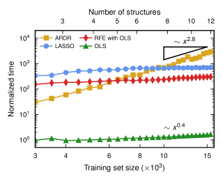
Several different methods were considered for constructing FC models for the Ta vacancy models, including OLS, RFE-OLS, LASSO, and ARDR. OLS is by far the computationally least expensive method and exhibits a favorable scaling with training set size (Fig. 1). (We note that scikit-learn employs the singular-value decomposition routine provided by scipy to solve the OLS problem, which in turn relies on lapack.) RFE-OLS and LASSO exhibit a very similar scaling as OLS but are about 100 to 500 times more expensive. This is unsurprising as these methods carry out multiple OLS optimizations as part of their algorithms. Finally, ARDR exhibits an unfavorable scaling with training set size (including both computational effort and memory requirements), which prevents its effective application for large sensing matrices including the present case.

Taking into account CV, the computational effort required for the largest supercells considered here becomes notable for LASSO and RFE-OLS. In the remainder of this section, we therefore primarily consider OLS, which will be demonstrated to work very well if combined with cutoff selection to avoid overfitting.

Furthermore, it is possible to tune parameters such as the rate at which the number of features is reduced in the RFE algorithm in each step, which effectively reduces the pre-factor of RFE. The present comparison focuses, however, on the ability of these methods to recover physically correct solutions and their convergence behavior, whence aspects concerning their computational performance are not further explored here.

Figure 2: Convergence with respect to parameter space for second-order Ta vacancy force constant models. The plot shows the variation of the root-mean-square error (RMSE) over training and validation sets with pair cutoff and hence the number of degrees of freedom in the model. Calculations were carried out using 15 training structures based on a $6\times 6\times 6$ conventional supercell, corresponding to a total of 19,395 force components. OLS: ordinary least squares; RFE: recursive feature elimination.

III.3 Cutoff selection via cross-validation

The number of DOFs in a FC model grows rapidly as the cutoff increases. At the same time, as discussed in subsubsection II.2.2, interaction strength and hence the magnitude of the FCs decay with increasing interatomic distance. At some point an increase in cutoff will therefore lead to negligible improvement in accuracy but merely an increase in model complexity. Specifically in the absence of regularization terms in the objective function ($\alpha=\beta=0$ in Eq. (2)), one can therefore observe a deterioration of model quality with the inclusion of more terms in the expansion due to overfitting. In this case one should therefore evaluate the performance of models with different cutoffs.

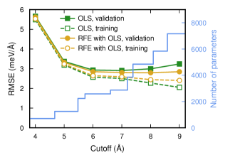
We employed CV using the shuffle-and-split method with 5 splits and 15 training structures for a system size of $N=6$ and constructed a series of second-order FC models with increasing cutoffs (Fig. 2). While the RMSE over the training set continues to decrease with increasing parameter space, the CV-RMSE has a minimum around 6 to 7 Å. For standard OLS the validation score increases for larger cutoffs due to overfitting. This behavior can be counteracted by using RFE, which yields a slight improvement of the CV-RMSE. As discussed above RFE is, however, computationally substantially more expensive whence OLS with a judicious choice of cutoffs is preferable. All subsequent analysis was therefore carried out using OLS and a second-order cutoff of 6 Å.

III.4 Convergence of thermodynamic properties

Figure 3: Convergence with training set size for thermodynamic properties from Ta vacancy force constant models. (a) Zone-center frequencies according to Eq. (4). (b) Free energy at 75% of the calculated melting temperature (2250 K) according to Eq. (5). (c) Elements of the second-order FC matrix according to Eq. (6). All calculations were carried out using a second-order cutoff radius of 6 Å (compare Fig. 2).

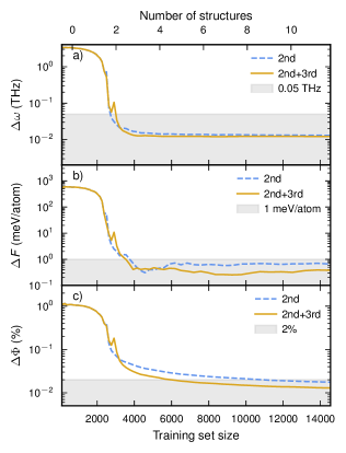
In order to evaluate how accurately the regression approach reproduces the correct second-order FCs, we considered three different measures. First, we evaluated the absolute error of the zone-center ($\Gamma$) frequencies obtained by regression relative to the direct approach (Fig. 3a),

$$\Delta\omega =\sqrt{\frac{1}{3N}\sum_{i}^{3N}(\omega_{\text{regression}}-\omega_{\mathrm{direct}})^{2}},$$ (4)

where $\omega_{i}$ is the frequency of mode $i$. Secondly, we considered the absolute difference in the harmonic free energy at 2250 K corresponding to 75% of the calculated melting temperature (Fig. 3b),

$$\Delta F =\left|F_{\text{regression}}^{\text{vib}}-F_{\text{direct}}^{\text{vib}}\right|.$$ (5)

Here, the free energies were computed within the harmonic approximation using phonopy Togo and Tanaka (2015).

Lastly, in order to obtain a computationally cheaper measure, we computed the relative error of the second-order FC matrices (Fig. 3c), defined as follows

$$\Delta\Phi =\|\Phi_{\text{regression}}-\Phi_{\text{direct}}\|\big{/}\|\Phi_{\text{regression}}\|$$ (6)

where $\|\ldots\|$ denotes the Frobenius norm.

The frequencies and free energies exhibit very similar convergence behavior. Both quantities reach convergence at about 3,000 force components, which is equivalent to two to three configurations and corresponds to the number of parameters in the model. Comparison with the measure based on the FC matrix itself, eq. (6), suggests that $\Delta\Phi\lesssim 5\%$ is sufficient to achieve convergence of the frequency spectrum and the free energy. Considering the convergence of $\Delta\Phi$ itself suggests a more conservative threshold of 2%.

The comparison includes both models with only second-order FCs terms and models with additional very short-ranged third-order FC terms using a cutoff of 3.0 Å. The latter perform consistently better than the second-order-only models. The inclusion of a few third-order terms thus stabilizes the extraction of the second-order FCs, an observation that has also been made in other situations Eriksson et al. (2019); Zhou et al. (2019a). These terms enable one to account for anharmonicity in the vicinity of the reference positions that would otherwise be effectively included in the second-order FCs. This principle can also be applied to higher-order terms, where we have found that adding a few terms of the respective next-higher order yields more accurate FCs.

III.5 Scaling with system size

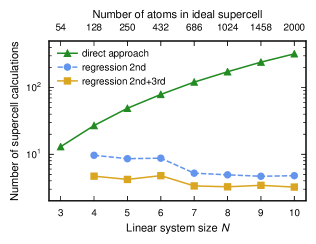
Following the analysis in the previous section, computing $\Delta\Phi$ as a function of the training set size allows one to determine the number of training structures needed for recovering the second-order FCs at the accuracy level of the direct approach (Fig. 4). Using the more conservative threshold of $\Delta\Phi<2\%$ (Fig. 3), we thereby determined the necessary number of supercell calculations as a function of system size (Fig. 4).

While in the direct approach the number of necessary calculations increases steeply with system size, in the regression approach it is constant or decreases slightly with system size. This is possible due to the introduction of a cutoff but more importantly since the regression takes advantage of the increase in information content with supercell size. In this context, it is important that all atoms are displaced by least a small amount. By contrast, the information content in configurations employed in the direct approach decreases substantially with system size as only one atom is displaced at a time. One can anticipate this scaling effect to be even more pronounced for third or higher-order FCs due to the exponential increase of the number of parameters with order Eriksson et al. (2019).

Figure 4: Size scaling when extracting second-order Ta vacancy force constant models. In the case of the regression approach, the force constant expansion include either second-order terms only or both second-order and a few (short-ranged) third-order terms.

IV Third-order force constants: Thermal conductivity

Calculating the thermal conductivity using the linearized Boltzmann transport equation requires knowledge of the second and third-order FCs Ziman (1960), providing a sensitive test for the extraction of higher-order FCs. Here, we analyze different regression methods for obtaining FCs and the resulting thermal conductivity in silicon. Specifically, we consider OLS, which has been used for the same purpose in Ref. Esfarjani and Stokes, 2008, LASSO, ad-LASSO, RFE-OLS, and ARDR as implemented in scikit-learn. This comparison enables us to demonstrate the importance of studying convergence with respect to the choice of cutoffs and number of training structures as well as the selection of a suitable fit method.

IV.1 Computational details

Reference second and third-order FCs were calculated for 250-atom supercells ($5\times 5\times 5$ primitive unit cells) via the direct approach using phonopy Togo and Tanaka (2015) and phono3py Togo et al. (2015), respectively. No cutoff was imposed during the calculation of the third-order FCs, which therefore required 801 individual force calculations.

For the regression approach, we generated a total of 20 reference structures based on 250-atom supercells ($5\times 5\times 5$ primitive unit cells) with displacements drawn from a normal distribution yielding an average displacement amplitude of 0.03 Å. For the computation of CV scores we used the same splits throughout to enable a one-to-one comparison of the regression methods.

Since ARDR exhibits a stronger scaling with system size than the other methods (Fig. 1), the pruning hyper-parameter $\lambda_{t}$ was not optimized but set to a constant value of $\lambda_{t}=10^{4}$.

For ARDR we first constructed a second-order-only model and then trained a second and third-order to the remaining forces. This $\Delta$-approach led to a significant improvement in accuracy and numerical stability for ARDR but did not improve the performance of the other fit methods.

For ad-LASSO the hyperparameter $\alpha$ was optimized once using CV and five training structures, after which the same value was used for all training set sizes. While one could thus possibly obtain slightly better results for larger training sets, the present choice allows a substantial reduction of the computational effort.

Reference forces were obtained from DFT calculations using the projector augmented wave method Blöchl (1994); Kresse and Joubert (1999) as implemented in vasp Kresse and Furthmüller (1996a, b) and an exchange-correlation functional Perdew et al. (1996) based on the generalized gradient approximation. The Brillouin zone was sampled using only the $\Gamma$-point. The plane-wave energy cutoff was set to 245 eV, an additional support grid for fast-Fourier transformations was used during the force calculation, and the projection operators were evaluated in reciprocal space.

IV.2 Optimization with cutoff selection

The number of DOFs associated with the second-order FCs is very small and thus we used the maximum cutoff range of 9.65 Å that the $5\times 5\times 5$ supercells employed here can support. The nearest neighbor fourth-order interaction, corresponding to a fourth-order cutoff of 2.5 Å, was included in order to improve the accuracy of the second and third-order FCs (as demonstrated in Sect. III). The third-order cutoff was then treated as a tunable parameter.

When using five training structures the accuracy of the model is already converged for a third-order cutoff of 4.0 Å (Fig. 5a) regardless of fit method, which yields a total of 80 DOFs. RFE-OLS and ARDR have, however, the distinct advantage of selecting fewer parameters and thus avoid overfitting for large cutoffs (Fig. 5b).

Figure 5: Comparison of third-order force constant models for Si constructed using a small parameter space. Convergence of (a) cross-validated root mean square error (RMSE) and (b) the number of features (non-zero parameters) with respect to third order cutoff using five training structures. Cutoffs of 9.65 and 2.5 Å were employed for second and fourth-order clusters, respectively. In ordinary least squares (OLS) no features are selected and hence in this case the number of features is identical to the total number of parameters. (c) Thermal conductivity at 300 K as a function of number of training structures using a third-order cutoff of 4.0 Å. ARDR: automatic relevance detection regression; LASSO: least absolute shrinkage and selection operator; RFE: recursive feature elimination.

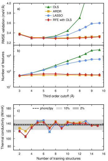
Using a third-order cutoff of 4.0 Å, the thermal conductivity converges to within 2% of the phono3py values using as few as 14 structures (Fig. 5). For comparison, the phono3py calculation requires 801 structures if no cutoff is imposed and 57 structures when including a pair cutoff of 4.0 Å (two neighbor shells). In the latter case, one must, however, take into account that convergence testing would require including at least one more shell, which increases the number of calculations to 95 (three neighbor shells).

For example, in the case of high-throughput studies one is often content with a less accurate estimate of the thermal conductivity. In this context, it is noteworthy that when using ARDR or RFE-OLS one converges to within 10% of the reference value already with four structures, while being able to test for convergence.

IV.3 Optimization with generic feature selection

Figure 6: Convergence of third-order force constant models for Si with training set size when using a large parameter space. Convergence of (a) cross-validated root mean square error (RMSE) and (b) the thermal conductivity at 300 K for generic feature selection methods as well as ordinary least squares (OLS) with respect to the number of training structures. Cutoffs of 9.65, 9.65 and 2.5 Å were employed for second, third and fourth-order clusters, respectively. ARDR: automatic relevance detection regression; LASSO: least absolute shrinkage and selection operator; RFE: recursive feature elimination.

Figure 7: Sparseness and accuracy of models obtained using different optimization methods. Variation of (a) the cross-validated root mean square error (RMSE) and (b) the thermal conductivity at 300 K with the number of features for Si third-order force constant models, constructed using five training structures and cutoffs of 9.65, 9.65 and 2.5 Å for second, third and fourth-order clusters, respectively. The number of features in each model was tuned via the hyperparameters of the respective optimization algorithms. The reference value for the thermal conductivity is shown by the dashed line in b and was computed using phono3py. ARDR: automatic relevance detection regression; LASSO: least absolute shrinkage and selection operator; RFE: recursive feature elimination.

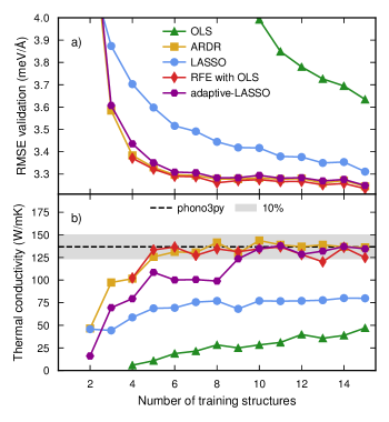
Cutoff selection can be thought as a feature selection approach, in which the cutoffs are pruning hyperparameters. In the present case, in which we focus on the third-order FCs we effectively obtain only one such hyperparameter, namely the third-order cutoff. The number of cutoff parameters increases with the expansion order and in more complex materials can require fine tuning e.g., between different atomic species or crystallographic sites Lindroth et al. (2019). In such situations it can be advantageous to employ generic feature selection algorithms. In this section, we consider the suitability of LASSO, ad-LASSO, RFE-OLS as well as ARDR for this purpose. For comparison, we also include the performance of OLS is included. Cutoffs of 9.65, 9.65, and 2.5 Å for second, third and fourth orders respectively were used throughout, which yields 2525 DOFs.

In the case of RFE-OLS and ARDR, the thermal conductivity converges to within 10% of the reference value using about five structures (Fig. 6b; see Supplementary Figure 2 for temperature dependence). Moreover, with ARDR one achieves convergence within 2% with about 12 structures, which is even better than in case of cutoff selection. In the case of LASSO and OLS, the convergence rate is considerably lower and neither method achieves convergence with respect to the reference value with the number of structures considered here.

We note that based on the convergence of the CV-RMSE scores (Fig. 6a) and the comparison with the cutoff selection study (Fig. 5a), one could expect LASSO to yield a reasonably converged thermal conductivity when using about 15 structures. This is not the case, demonstrating that CV-RMSE scores alone are insufficient for assessing the quality of a model. Information criteria such as alkaline information criteria (AIC) and Bayesian information criterion (BIC) can be used to evaluate models Akaike (1974); Schwarz (1978); Aho et al. (2014), taking into account the predictive power but also penalizing the number of parameters of the model. These types of measure may serve as a useful compliment to the CV score when evaluating FC models. They were, for example, used recently to evaluate alloy cluster expansion models Zhang et al. (2020).

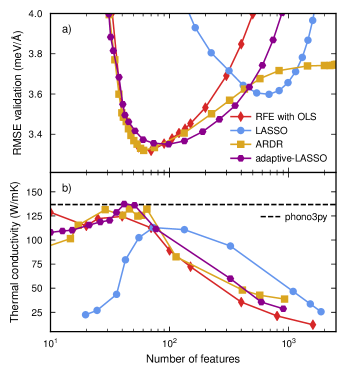
To explore the differences in performance between LASSO, RFE-OLS, and ARDR further we explicitly computed the CV-RMSE as a function of their respective pruning hyperparameter using five training structures, which allows us to obtain the variation of the CV score with the number of features (Fig. 7a). While the methods achieve comparable RMSE scores, the optimal LASSO solution contains a much larger number of features. The tendency of (standard) LASSO to over-select is known Zou (2006) and we have observed this behavior also in other applications such as alloy cluster expansions Ångqvist et al. (2019). A physical understanding of the shortcoming of LASSO is obtained by inspecting the FCs directly (Fig. 8). The second-order FCs are very similar for all methods (not shown) but notable differences are observed in the third-order FCs. While RFE-OLS and ARDR produce a small number of short-ranged interaction terms, LASSO yields a large number of spurious third-order FCs terms (see Supplementary Figure 2).

Figure 8: Ability of different optimization methods to recover the correct third-order force constants. Norm of third-order force constants in Si obtained using generic feature selection algorithms and ten training structures. Cutoffs of 9.65, 9.65 and 2.5 Å were employed for second, third and fourth-order clusters, respectively. The cluster radius is defined as $r_{c}=\sum_{i\in\text{cluster}}\left\|\mathbf{r}_{i}-\mathbf{r}_{gc}\right\|\big{/}N$ where $\mathbf{r}_{gc}$ is the geometrical center of the cluster (compare Supplementary Figure 2). ARDR: automatic relevance detection regression; LASSO: least absolute shrinkage and selection operator; RFE: recursive feature elimination.

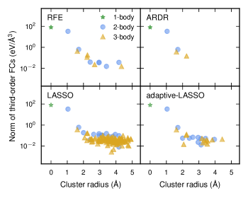
The over-selection in LASSO can be overcome by using, e.g., ad-LASSO, see Eq. (3) Zou (2006). This yields a learning curve comparable to ARDR (Fig. 6a) and a much smaller number of features compared to LASSO (Fig. 7a). Thereby, one obtains a small set of third-order terms (Fig. 8) that properly reproduce the physical properties of the system (Fig. S2).

It is striking that all techniques except for LASSO can achieve convergence of the thermal conductivity to within 5% with only five training structures (Fig. 7b). It is also noteworthy that the CV score alone is an unreliable predictor for model quality. This is especially apparent in the case of LASSO, for which the model with the smallest CV score leads to an underestimation of the thermal conductivity by 50%. Using the CV score alone for model selection can hence be very misleading. For this purpose, one could therefore also consider model evaluation metrics such as AIC and BIC– an aspect that deserves further study.

Finally, we note that overestimating the true number of features leads to very large errors in the predicted thermal conductivity for all techniques. Underestimation on the other hand, i.e. overly sparse models, give much smaller errors, which indicates that over-regularization is the preferable mode of error.

We emphasize that the data sets used here are publicly available git (2 18) and can serve as a test bed for a systematic comparison with respect to other fit algorithms and feature selection methods.

V Fourth-order force constants: Strong anharmonicity

Figure 9: Fourth-order FC models for Ba₈Ga₁₆Ge₃₀. (a) Comparison of cross-validated root mean square error (RMSE) and number of features for the models defined in Table 1. (b) Predicted vs target forces and (c) norm of the force constants (FCs) for Model 4. LASSO: least absolute shrinkage and selection operator; OLS: ordinary least squares; RFE: recursive feature elimination.

In this section, we are concerned with the inorganic clathrate Ba₈Ga₁₆Ge₃₀, in which the motion of Ba atoms is strongly anharmonic Madsen and Santi (2005). This manifests itself in a strong temperature dependence of vibrational modes associated with Ba Christensen et al. (2008) and moreover has implications for the thermal conductivity Christensen et al. (2008); Tadano and Tsuneyuki (2018b); Lindroth et al. (2019). While perturbation theory formally provides an expression for the temperature induced phonon frequency shifts caused by the third-order FC terms Wallace (1998), one commonly carries the expansion at least to the next higher even order, when analyzing frequency shifts Errea et al. (2014); Tadano and Tsuneyuki (2018b); Lindroth et al. (2019). Since Ba₈Ga₁₆Ge₃₀ has a large unit cells, it thus serves as an example for a system, in which both higher-order FCs are required and the number of DOFs is very large.

Clathrates are inclusion compounds with a defined lattice structure that can trap atomic or small molecular species. Ba₈Ga₁₆Ge₃₀ belongs to the class of type-I clathrates with spacegroup Pm$\bar{3}$n Shevelkov and Kovnir (2011). In this case, the host lattice is made up of Ga and Ge atoms, which occupy Wyckoff sites $6c$, $16i$, and $24k$, whereas Ba atoms reside inside the cages occupying Wyckoff sites $2a$ and $6d$. Due to the size mismatch between guest species and cages, which is particular large for the $6d$ sites, the Ba atoms experience a very wide and flat PES with pronounced anharmonicity. In earlier work, we analyzed the ordering of the host species and extracted the ordered ground state structure of Ba₈Ga₁₆Ge₃₀ Ångqvist et al. (2016); Ångqvist and Erhart (2017), which serves as a prototype structure for the analysis of the FCs.

V.1 Calculation of reference forces

Reference forces were obtained for the 54-atom cells described below from DFT calculations using the computational approach described in subsection IV.1. The exchange-correlation potential was represented using the vdW-DF-cx method, which combines semi-local exchange with non-local correlation Dion et al. (2004); Klimes̆ et al. (2011); Berland and Hyldgaard (2014), as it has been previously shown to provide a good description of the vibrational modes of this system Lindroth et al. (2019). The Brillouin zone was sampled using a $\Gamma$-centered $3\times 3\times 3$ $\mathbf{k}$-point mesh and the plane-wave energy cutoff was set to 243 eV.

Table 1: Fourth-order FC models for Ba₈Ga₁₆Ge₃₀ obtained by OLS using different combinations of cutoffs and expansion orders.

Model	Two-body cutoffs						Three-body cutoffs
	2${}^{\text{nd}}$	3${}^{\text{rd}}$	4${}^{\text{th}}$	5${}^{\text{th}}$	6${}^{\text{th}}$		3${}^{\text{rd}}$	4${}^{\text{th}}$ order
1	$5.4$	$3.0$	$3.0$
2	$5.4$	$3.5$	$3.5$
3	$5.4$	$4.0$	$4.0$
4	$5.4$	$4.35$	$4.35$
5	$5.4$	$4.7$	$4.7$
6	$5.4$	$4.35$	$4.35$	$3.0$	$3.0$
7	$5.4$	$4.35$	$4.35$				$4.0$	$4.0$

V.2 Model construction

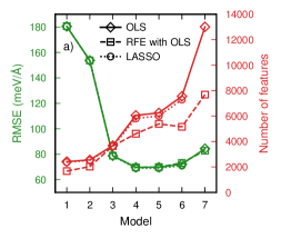
First, we generated 50 structures based on the primitive 54-atom unit cell with an average displacement amplitude of 0.28 Å using the Monte Carlo rattle approach described in Ref. Eriksson et al., 2019. These structures were used to train an initial fourth-order model, which was subsequently sampled by MD simulations at 300 and 650 K for 10 ps. We extracted 50 structures from each runs and generated reference forces via DFT calculations. Thereby we obtained a total of 150 reference structures and thus a sensing matrix with 24,300 rows. Due to the large number of DOFs in this structure (Table 1) the computational effort that has to be expended for training models becomes very significant. For illustration, a OLS fit with 10-fold CV of the largest model considered below requires approximately one hour on an Intel Xeon E5-2650 V3 CPU. Given the scaling analysis above (Fig. 1) this translates to several days and more when using RFE-OLS or LASSO. Since the computational effort associated with ad-LASSO is yet another order of magnitude larger than for LASSO, we restricted ourselves to OLS, RFE-OLS, and (standard) LASSO, the latter of which has been previously used for a very similar structure Tadano and Tsuneyuki (2018b). We constructed several different models and evaluated their performance by CV in order to identify a suitable combination of expansion order and cutoff parameters (Table 1).

Figure 10: Potential energy landscape for Ba atoms located at 2a and 6d Wyckoff sites along the $\left<111\right>$ direction. The potential energy surfaces along $\left<100\right>$ and $\left<110\right>$ are shown in Supplementary Figure 5.

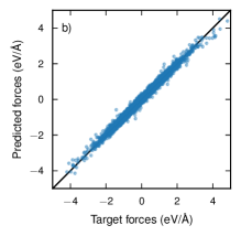
The three optimization methods considered here yield virtually identical CV-RMSE scores (Fig. 9a), which is sensible as even for the largest cutoff parameters the number of DOFs is still significantly smaller than the number of rows in the sensing matrix (Table 1). RFE-OLS and to a very slight extent also LASSO yield a smaller number of features. In practice, one has to balance this advantage (which can also imply shorter run times for force evaluations of the final model) against the additional effort required for construction of the model. Based on the good scores that can already be obtained with OLS and the fact that these cases are commonly easy to move into the overdetermined region, even for spaces as large as in the present case, one can argue that OLS is often the more natural choice. In the following, we therefore restrict our analysis to the OLS fits.

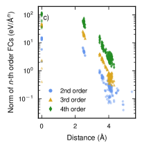
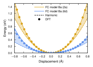
The smallest CV-RMSE score is obtained for model 4 (Fig. 9a), which yields a value of 68 meV/Å to be compared with maximum force components of about 4000 meV/Å (Fig. 9b). The fourth-order cutoff for this model is 4.35 Å, which is enough to include all Ba-cage interactions indicating that the anharmonicity of all of these interactions is important. The PES for Ba atoms along different directions calculated is in excellent agreement with DFT calculations (Fig. 10). It is apparent that Ba atoms in 6d sites behave more anharmonic than those in 2a sites, as the cages surrounding the former are larger.

To analyze the behavior of model 4 further, we generated an ensemble of FC models that are trained in identical fashion but are based on different training sets. The latter were constructed by selection with replacement (bagging) from the available data set such that the number of reference forces in the training sets equals the total size of the data set. The RMSEs over the training set obtained for these FC models are similar to model 4. This ensemble of models enabled us to estimate the sensitivity for predictions for physical properties such as phonon frequencies (Fig. 11) and thermal conductivity (Fig. 12).

V.3 Thermal conductivity

The low thermal conductivity of inorganic clathrates is often attributed to the rattling motion of the guest species Madsen and Santi (2005); Christensen et al. (2008). These modes exhibit a notable temperature dependence Christensen et al. (2008) that needs to be accounted for in order to predict the thermal conductivity accurately Tadano and Tsuneyuki (2018b); Lindroth et al. (2019). The common approach to Boltzmann transport theory, however, only considers terms up to third-order and neglects the temperature dependence of the phonon frequencies. The fourth-order model allows us to investigate the temperature dependence of the frequency spectrum and include this effect when calculating the thermal conductivity via the temperature dependent force constants approach Andersson (2012); Hellman and Abrikosov (2013); Lindroth et al. (2019). Yet instead of training effective third-order models from ab-initio MD simulations, we train them against snapshots and forces generated from MD simulations using the full fourth order model. The latter simulations were carried out using a supercell of $2\times 2\times 2$ primitive unit cells (432 atoms). The systems was first equilibrated for 10 ps using a Langevin thermostat as implemented in ASE Larsen et al. (2017). Subsequently, the simulations were continued in the micro-canonical ensemble for another 5 ps. From the latter part, 100 snapshots were selected to train effective second and third-order FCs.

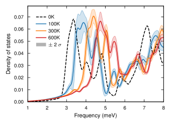
The density of states (DOS) obtained from the effective second-order FCs reveals a significant temperature dependence of the low-frequency Ba modes around 4 meV (Fig. 11), in line with experimental work Christensen et al. (2008) and our previous study, which was based on ab-initio MD simulations Lindroth et al. (2019). The sensitivity analysis (see subsection V.2) shows that the dependence of the DOS on model uncertainty is considerably weaker than the temperature dependence. We also note that the DOS has a slightly weaker temperature dependency if the harmonic force constants are trained without including the third-order FCs. This is in qualitative agreement with the negative frequency shift due to cubic force constants observed in Ref. Tadano and Tsuneyuki, 2018b.

Figure 11: Temperature dependent phonon density of states for Ba₈Ga₁₆Ge₃₀ from effective second-order force constants. Shaded regions indicate $\pm 2\sigma$, for each respective temperature, obtained from the sensitivity analysis described in the text.

Figure 12: Thermal conductivity for Ba₈Ga₁₆Ge₃₀ computed from the linearized Boltzmann transport equation. Data shown by solid blue lines and open black square taken from Ref. Lindroth et al., 2019. Shaded regions indicate $\pm 10\sigma$, for each respective temperature, obtained from the sensitivity analysis described in the text. TDIFCs: temperature-dependent interatomic force constants.

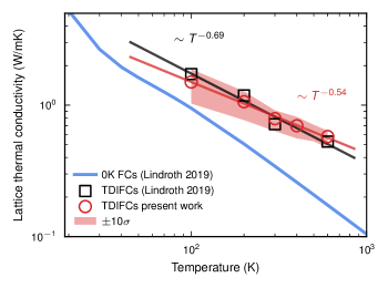
The effective FCs were furthermore used to extract the thermal conductivity at the respective temperature they were trained using the linearized Boltzmann transport equation via shengBTE Li et al. (2014). The resulting thermal conductivity is in very good agreement with our previous calculations (Fig. 12), which were based on full ab-initio MD simulations and which in turn agrees well with experimental results Lindroth et al. (2019). We note that as shown in Refs. Tadano and Tsuneyuki, 2018b and Lindroth et al., 2019, the thermal conductivity is strongly underestimated when using the temperature-independent (zero-K) second and third-order FCs as that approach fails to account for the strong renormalization with temperature of the lowest-frequency heat carrying modes. As in the case of the DOS, the model sensitivity analysis reveals a very weak variation in thermal conductivity due to model uncertainty.

The very good agreement with the results obtained using temperature-dependent interatomic force constants trained using ab-initio MD simulations demonstrates that our fourth-order model provides an accurate and transferable description of the PES in the temperature range of interest. The effective models in the present work, however, required only a fraction of the computer time that was needed for the ab-initio MD simulations in Ref. Lindroth et al., 2019.

The present results are also in semi-quantitative agreement with the results from Ref. Tadano and Tsuneyuki, 2018b, which were obtained using a Green’s function approach for treating phonon renormalization. The latter calculations were carried using a different structural model that does not correspond to a thermally accessible state, whence one cannot expect quantitative agreement. There are further methodological differences between the Green’s function approach in Ref. Tadano and Tsuneyuki, 2018b and the present work. The latter takes into account quantum statistic but only handles renormalization of the second-order FCs, whereas the present approach is classical but effectively accounts for higher-order terms via temperature-dependent third-order FCs Lindroth et al. (2019).

VI Discussion

Regression techniques can reduce the computational effort associated with FC extraction compared to enumeration techniques by one or more orders of magnitude, in particular in the case of higher-order expansions and/or large systems with low symmetry. In this study, we have therefore assessed both efficiency and efficacy of several regression methods in different application scenarios. Specifically, we considered second-order FCs and derived properties for large systems (Sect. III), third-order FCs and thermal conductivity (Sect. IV) as well as fourth and higher-order FCs and their sampling for strongly anharmonic systems (Sect. V and Supplementary Information).

While the discussion below is explicitly based on the results presented in the preceding sections, they are further supported by our experience with various other materials including, e.g., metals, oxides, carbides, and chalcogenides of varying dimensionality including two and three-dimensional systems, interfaces, and defects. Hence, we consider our conclusions to be applicable to other materials and application areas to a reasonable extent.

VI.1 Second-order FCs in large systems

For second-order FCs in large systems the regression approach can reduce the computational effort by more than one order of magnitude compared to the direct approach (Fig. 4). OLS with cutoff selection yields prediction errors that are on par with more advanced regression techniques such as RFE-OLS, LASSO, or ARDR. The latter are, however, at least one to two orders of magnitude more demanding in terms of computer time, which can become a concern for very large systems.

For OLS to work properly the linear system to be solved must be overdetermined. The configurations used for regression can be obtained by rattling the atomic positions. As a result, the information density, i.e. the number of force components that are sizable, is high, which is usually not the case for enumerated structures such as the ones used in the direct approach. As a result, a much smaller number of configurations is required in order to obtain a well conditioned sensing matrix.

We have furthermore found that inclusion of a few higher-order FC terms (here third-order FCs with a short cutoff) accelerates convergence of the lower-order FCs of interest with respect to training set size. Here, the third-order terms allow extraction of the “true” second-order expansion terms, which otherwise would have to effectively account for anharmonicity in the PES.

VI.2 Third-order FCs and thermal conductivity

The regression approach also drastically reduces the number of reference calculations needed to recover the parameters of third-order FC expansions. Here, care must be taken to verify not only the convergence of the CV-RMSE scores with respect to the references forces but to consider the actual property of interest, in the present case the thermal conductivity.

As shown previously Esfarjani and Stokes (2008), OLS with cutoff selection provides a viable route to obtaining well-converged thermal conductivity values at a fraction of the computational cost of the direct approach. Several generic feature selection methods provide, however, viable alternatives that require adjusting a smaller number of hyperparameters and are hence more easily extensible to complex systems and higher-order expansions.

Here, RFE-OLS, ARDR, and ad-LASSO have been found to work very reliably and efficiently, yielding both fast convergence and a small number of features (sparse solutions). Standard LASSO produces denser solutions, which leads to less predictive models and has a detrimental impact when predicting the thermal conductivity.

VI.3 Higher-order FC models and anharmonic PESs

We also considered the construction of FC expansions beyond third-order, which is usually impractical with enumeration approaches. Specifically, we constructed fourth-order FC models with up to more than 13,000 parameters for the inorganic clathrate Ba₈Ga₁₆Ge₃₀ using OLS with cutoff selection. Using the final model effective FCs were generated and used to compute the temperature dependent DOS and thermal conductivity, yielding results in agreement with experiment as well as previous computational work.

These results demonstrate that the “standard” and computationally relatively cheap OLS method can be used to capture strongly anharmonic effects across a wide temperature range. It can easily be extend to higher order anharmonicity and properties other than the thermal conductivity, as shown by an eighth-order model for a Ni surface, which allows one to model the temperature dependence of the surface layer spacing (see Supplementary Information).

To put the present results in context, we note that the benefits of regression with regularization, typically discussed under the heading of CS, have been particularly emphasized for systems with many DOFs, which includes both the clathrate system (over 13,000 parameters) and the Ni surface (2,000 parameters) considered here. While for other linear models, specifically cluster expansions, it can be difficult to generate that many reference data points, for FC expansions generating reference data is relatively easy and often simpler than tuning of model parameters and hyperparameters. For example, for the clathrate system, one structure provides 162 reference force components and hence already with less than a hundred such structures one obtains an overdetermined system.

One could argue that regularization would allow one to reduce the number of reference data points considerably, making techniques such as ad-LASSO, LASSO or even ARDR competitive. In this regard, we point out that the RFE-OLS fits for the clathrate system show that a sensible model has about 4000 to 5000 parameters. Even with regularization, one should thus require approximately as many reference data points, which is often not a substantial enough reduction to warrant the substantially larger computational effort associated with regularization techniques.

VII Conclusions and outlook

Generic feature selection algorithms, in particular ARDR, RFE, and ad-LASSO can yield physically-sound FC expansions at a fraction of the cost of enumeration approaches. This approach can be very powerful as demonstrated here for extracting third-order FCs and thermal conductivity. The application of (standard) LASSO approach is, however, not indicated due to its tendency to over-select, which leads to very slow convergence with training set size. For large unit cells with low symmetry and/or high-order expansions these techniques come, however, with a non-negligible cost that can be more than two orders of magnitude higher than that of OLS. The cost is still much smaller than those of DFT calculations but since the underlying problem is not as amenable to parallelization it can still become a factor to consider in practice. In such cases OLS with cutoff selection provides a viable route, with trivial parallelization over multiple cutoff parameter sets. The viability of the latter approach has been demonstrated here for both second-order FCs in large low-symmetry unit cells and high-order FCs in low-symmetry systems.

Regression techniques are in principle very attractive for high-throughput schemes, since they require much less computational effort than enumeration approaches. For the regression approach to be viable one must, however, not only consider the computational effort but also the amount of human intervention required. In the future, it is therefore desirable to set up protocols that automatically construct and validate FC models.

Finally, we have made the data related to the analysis of higher-order FC expansions publicly available git (2 18) to provide a standardized benchmark set for future work.

Data and code availability

The data and code related to the analysis of third-order models in Si and fourth-order models in Ba₈Ga₁₆Ge₃₀ is publicly available in the form of a gitlab repository at https://gitlab.com/materials-modeling/hiphive-examples.

References

- Esfarjani and Stokes (2008) K. Esfarjani and H. T. Stokes, Method to extract anharmonic force constants from first principles calculations, Phys. Rev. B 77, 144112 (2008).
- Esfarjani and Liang (2020) K. Esfarjani and Y. Liang, Thermodynamics of anharmonic lattices from first-principles, in Nanoscale Energy Transport, edited by B. Liao (IOP Publishing Ltd, Bristol, England, 2020) Chap. 7.
- Candes and Wakin (2008) E. Candes and M. Wakin, An introduction to compressive sampling, Signal Processing Magazine, IEEE 25, 21 (2008).
- Nelson et al. (2013a) L. J. Nelson, G. L. W. Hart, F. Zhou, and V. Ozoliņš, Compressive sensing as a new paradigm for model building, Phys. Rev. B 87, 035125 (2013a).
- Tadano and Tsuneyuki (2015) T. Tadano and S. Tsuneyuki, Self-consistent phonon calculations of lattice dynamical properties in cubic SrTiO3 with first-principles anharmonic force constants, Phys. Rev. B 92, 054301 (2015).
- Nelson et al. (2013b) L. J. Nelson, V. Ozoliņš, C. S. Reese, F. Zhou, and G. L. W. Hart, Cluster expansion made easy with Bayesian compressive sensing, Phys. Rev. B 88, 155105 (2013b).
- Zhou et al. (2014) F. Zhou, W. Nielson, Y. Xia, and V. Ozoliņš, Lattice anharmonicity and thermal conductivity from compressive sensing of first-principles calculations, Phys. Rev. Lett. 113, 185501 (2014).
- Ångqvist et al. (2016) M. Ångqvist, D. O. Lindroth, and P. Erhart, Optimization of the thermoelectric power factor: Coupling between chemical order and transport properties, Chem. Mater. 28, 6877 (2016).
- Zhou et al. (2019a) F. Zhou, W. Nielson, Y. Xia, and V. Ozoliņš, Compressive sensing lattice dynamics. I. general formalism, Phys. Rev. B 100, 184308 (2019a).
- Zhou et al. (2019b) F. Zhou, B. Sadigh, D. Åberg, Y. Xia, and V. Ozoliņš, Compressive sensing lattice dynamics. II. Efficient phonon calculations and long-range interactions, Phys. Rev. B 100, 184309 (2019b).
- Plata et al. (2017) J. J. Plata, P. Nath, D. Usanmaz, J. Carrete, C. Toher, M. de Jong, M. Asta, M. Fornari, M. B. Nardelli, and S. Curtarolo, An efficient and accurate framework for calculating lattice thermal conductivity of solids: AFLOW–AAPL Automatic Anharmonic Phonon Library, npj Comp. Mater. 3, 45 (2017).
- Grimvall (1999) G. Grimvall, Thermophysical Properties of Materials (North Holland, Amsterdam, 1999).
- Grimvall et al. (2012) G. Grimvall, B. Magyari-Köpe, V. Ozoliņš, and K. A. Persson, Lattice instabilities in metallic elements, Rev. Mod. Phys. 84, 945 (2012).
- Wallace (1998) D. C. Wallace, Thermodynamics of Crystals (Dover, Mineola, New York, 1998).
- Eriksson et al. (2019) F. Eriksson, E. Fransson, and P. Erhart, The hiphive package for the extraction of high-order force constants by machine learning, Adv. Simul. Theo. 2, 1800184 (2019).
- Agoston and Albe (2009) P. Agoston and K. Albe, Formation entropies of intrinsic point defects in cubic In2O3 from first-principles density functional theory calculations, Phys. Chem. Chem. Phys. 11, 3226 (2009).
- Şopu et al. (2011) D. Şopu, J. Kotakoski, and K. Albe, Finite-size effects in the phonon density of states of nanostructured germanium: A comparative study of nanoparticles, nanocrystals, nanoglasses, and bulk phases, Phys. Rev. B 83, 245416 (2011).
- Katre et al. (2017) A. Katre, J. Carrete, B. Dongre, G. K.-H. Madsen, and N. Mingo, Exceptionally strong phonon scattering by B substitution in cubic SiC, Phys. Rev. Lett. 119, 075902 (2017).
- Thomas and der Ven (2013) J. C. Thomas and A. V. der Ven, Finite-temperature properties of strongly anharmonic and mechanically unstable crystal phases from first principles, Phys. Rev. B 88, 214111 (2013).
- Hellman et al. (2011) O. Hellman, I. A. Abrikosov, and S. I. Simak, Lattice dynamics of anharmonic solids from first principles, Phys. Rev. B 84, 180301 (2011).
- Hellman et al. (2013) O. Hellman, P. Steneteg, I. A. Abrikosov, and S. I. Simak, Temperature dependent effective potential method for accurate free energy calculations of solids, Phys. Rev. B 87, 104111 (2013).
- Tadano et al. (2014) T. Tadano, Y. Gohda, and S. Tsuneyuki, Anharmonic force constants extracted from first-principles molecular dynamics: applications to heat transfer simulations, J. Phys. Cond. Matter 26, 225402 (2014).
- hip (2 01) https://hiphive.materialsmodeling.org/ (Accessed: 2019-12-01).
- Parlinski et al. (1997) K. Parlinski, Z. Q. Li, and Y. Kawazoe, First-principles determination of the soft mode in cubic ZrO2, Phys. Rev. Lett. 78, 4063 (1997).
- Togo and Tanaka (2015) A. Togo and I. Tanaka, First principles phonon calculations in materials science, Scr. Mater. 108, 1 (2015).
- Togo et al. (2015) A. Togo, L. Chaput, and I. Tanaka, Distributions of phonon lifetimes in Brillouin zones, Phys. Rev. B 91, 094306 (2015).
- Li et al. (2014) W. Li, J. Carrete, N. A. Katcho, and N. Mingo, ShengBTE: A solver of the Boltzmann transport equation for phonons, Comp. Phys. Comm. 185, 1747 (2014).
- Carrete et al. (2017) J. Carrete, B. Vermeersch, A. Katre, A. van Roekeghem, T. Wang, G. K. H. Madsen, and N. Mingo, almaBTE : A solver of the space–time dependent Boltzmann transport equation for phonons in structured materials, Comp. Phys. Comm. 220, 351 (2017).
- Madsen and Santi (2005) G. K. H. Madsen and G. Santi, Anharmonic lattice dynamics in type-I clathrates from first-principles calculations, Phys. Rev. B 72, 220301 (2005).
- Lindroth et al. (2019) D. O. Lindroth, J. Brorsson, E. Fransson, F. Eriksson, A. Palmqvist, and P. Erhart, Thermal conductivity in intermetallic clathrates: A first-principles perspective, Phys. Rev. B 100, 045206 (2019).
- Esfarjani et al. (2011) K. Esfarjani, G. Chen, and H. T. Stokes, Heat transport in silicon from first-principles calculations, Phys. Rev. B 84, 085204 (2011).
- Tadano and Tsuneyuki (2018a) T. Tadano and S. Tsuneyuki, First-principles lattice dynamics method for strongly anharmonic crystals, J. Phys. Soc. Japan 87, 041015 (2018a).
- Tadano and Tsuneyuki (2018b) T. Tadano and S. Tsuneyuki, Quartic anharmonicity of rattlers and its effect on lattice thermal conductivity of clathrates from first principles, Phys. Rev. Lett. 120, 105901 (2018b).
- Andersson (2012) T. Andersson, Master’s thesis, Chalmers University of Technology, Gothenburg, Sweden (2012), One-shot free energy calculations for crystalline materials.
- Note (1) One should emphasize that the rows of the sensing matrix in Eq. (1\@@italiccorr) are always to some extent correlated due to atomic interactions as each row corresponds to the Cartesian force component of one atom in one structure. This should be kept in mind when using the terms overdetermined and underdetermined in the usual sense that is based on the relation between the number of rows and columns of the sensing matrix.
- Zou (2006) H. Zou, The adaptive Lasso and its oracle properties, J. Amer. Stat. Assoc. 101, 1418 (2006).
- Gramfort (2012) A. Gramfort, https://gist.github.com/agramfort/1610922 (2012).
- Pedregosa et al. (2011) F. Pedregosa et al., Scikit-learn: Machine learning in Python, J. Machine Learn. Res. 12, 2825 (2011).
- Dongre et al. (2018) B. Dongre, J. Carrete, A. Katre, N. Mingo, and G. K. H. Madsen, Resonant phonon scattering in semiconductors, J. Mater. Chem. C 6, 4691 (2018).
- Kundu et al. (2019) A. Kundu, F. Otte, J. Carrete, P. Erhart, W. Li, N. Mingo, and G. K. H. Madsen, Effect of local chemistry and structure on thermal transport in doped GaAs, Phys. Rev. Mater. 3, 094602 (2019).
- Alkauskas et al. (2014) A. Alkauskas, B. B. Buckley, D. D. Awschalom, and C. G. V. de Walle, First-principles theory of the luminescence lineshape for the triplet transition in diamond nv centres, New J. Phys. 16, 073026 (2014).
- Shang et al. (2020) Z. Shang, A. Hashemi, Y. Berencén, H.-P. Komsa, P. Erhart, S. Zhou, M. Helm, A. V. Krasheninnikov, and G. V. Astakhov, Local vibrational modes of Si vacancy spin qubits in SiC, Phys. Rev. B 101, 144109 (2020).
- Ravelo et al. (2013) R. Ravelo, T. C. Germann, O. Guerrero, Q. An, and B. L. Holian, Shock-induced plasticity in tantalum single crystals: Interatomic potentials and large-scale molecular-dynamics simulations, Phys. Rev. B 88, 134101 (2013).
- Ziman (1960) J. M. Ziman, Electrons and phonons (Oxford University Press, Oxford, 1960).
- Blöchl (1994) P. E. Blöchl, Projector augmented-wave method, Phys. Rev. B 50, 17953 (1994).
- Kresse and Joubert (1999) G. Kresse and D. Joubert, From ultrasoft pseudopotentials to the projector augmented-wave method, Phys. Rev. B 59, 1758 (1999).
- Kresse and Furthmüller (1996a) G. Kresse and J. Furthmüller, Efficiency of ab-initio total energy calculations for metals and semiconductors using a plane-wave basis set, Comp. Mater. Sci. 6, 15 (1996a).
- Kresse and Furthmüller (1996b) G. Kresse and J. Furthmüller, Efficient iterative schemes for ab initio total-energy calculations using a plane-wave basis set, Phys. Rev. B 54, 11169 (1996b).
- Perdew et al. (1996) J. P. Perdew, K. Burke, and M. Ernzerhof, Generalized gradient approximation made simple, Phys. Rev. Lett. 77, 3865 (1996).
- Akaike (1974) H. Akaike, A new look at the statistical model identification, IEEE Transactions on Automatic Control 19, 716 (1974).
- Schwarz (1978) G. Schwarz, Estimating the dimension of a model, The Annals of Statistics 6, 461 (1978).
- Aho et al. (2014) K. Aho, D. Derryberry, and T. Peterson, Model selection for ecologists: The worldviews of AIC and BIC, Ecology 95, 631 (2014).
- Zhang et al. (2020) J. Zhang, X. Liu, S. Bi, J. Yin, G. Zhang, and M. Eisenbach, Robust data-driven approach for predicting the configurational energy of high entropy alloys, Materials & Design 185, 108247 (2020).
- Ångqvist et al. (2019) M. Ångqvist, W. A. Muñoz, J. M. Rahm, E. Fransson, C. Durniak, P. Rozyczko, T. H. Rod, and P. Erhart, icet - A Python library for constructing and sampling alloy cluster expansions, Adv. Simul. Theo. 2, 1900015 (2019).
- git (2 18) https://gitlab.com/materials-modeling/hiphive-examples (Accessed: 2019-12-18).
- Christensen et al. (2008) M. Christensen, A. B. Abrahamsen, N. B. Christensen, F. Juranyi, N. H. Andersen, K. Lefmann, J. Andreasson, C. R. H. Bahl, and B. B. Iversen, Avoided crossing of rattler modes in thermoelectric materials, Nat. Mater. 7, 811 (2008).
- Errea et al. (2014) I. Errea, M. Calandra, and F. Mauri, Anharmonic free energies and phonon dispersions from the stochastic self-consistent harmonic approximation: Application to platinum and palladium hydrides, Phys. Rev. B 89, 064302 (2014).
- Shevelkov and Kovnir (2011) A. V. Shevelkov and K. Kovnir, Zintl clathrates, in Zintl phases, Structure and Bonding, edited by T. F. Fässler (Springer, Heidelberg, 2011) p. 97.
- Ångqvist and Erhart (2017) M. Ångqvist and P. Erhart, Understanding chemical ordering in intermetallic clathrates from atomic scale simulations, Chem. Mater. 29, 7554 (2017).
- Dion et al. (2004) M. Dion, H. Rydberg, E. Schröder, D. C. Langreth, and B. I. Lundqvist, Van der Waals density functional for general geometries, Phys. Rev. Lett. 92, 246401 (2004).
- Klimes̆ et al. (2011) J. Klimes̆, D. R. Bowler, and A. Michaelides, Van der Waals density functionals applied to solids, Phys. Rev. B 83, 195131 (2011).
- Berland and Hyldgaard (2014) K. Berland and P. Hyldgaard, Exchange functional that tests the robustness of the plasmon description of the van der Waals density functional, Phys. Rev. B 89, 035412 (2014).
- Hellman and Abrikosov (2013) O. Hellman and I. A. Abrikosov, Temperature-dependent effective third-order interatomic force constants from first principles, Phys. Rev. B 88, 144301 (2013).
- Larsen et al. (2017) A. H. Larsen et al., The atomic simulation environment — a Python library for working with atoms, J. Phys. Cond. Matter 29, 273002 (2017).