PIPPS: Flexible Model-Based Policy Search
Robust to the Curse of Chaos

Abstract

Previously, the exploding gradient problem has been explained to be central in deep learning and model-based reinforcement learning, because it causes numerical issues and instability in optimization. Our experiments in model-based reinforcement learning imply that the problem is not just a numerical issue, but it may be caused by a fundamental chaos-like nature of long chains of nonlinear computations. Not only do the magnitudes of the gradients become large, the direction of the gradients becomes essentially random. We show that reparameterization gradients suffer from the problem, while likelihood ratio gradients are robust. Using our insights, we develop a model-based policy search framework, Probabilistic Inference for Particle-Based Policy Search (PIPPS), which is easily extensible, and allows for almost arbitrary models and policies, while simultaneously matching the performance of previous data-efficient learning algorithms. Finally, we invent the total propagation algorithm, which efficiently computes a union over all pathwise derivative depths during a single backwards pass, automatically giving greater weight to estimators with lower variance, sometimes improving over reparameterization gradients by $10^{6}$ times.

1 Introduction

(a) Analytic approximation

(b) Particle approximation

Figure 1: One can either perform extensive mathematical derivations to analytically predict an approximate trajectory distribution, or use a flexible particle approach to predict a stochastic approximation to the true trajectory distribution.

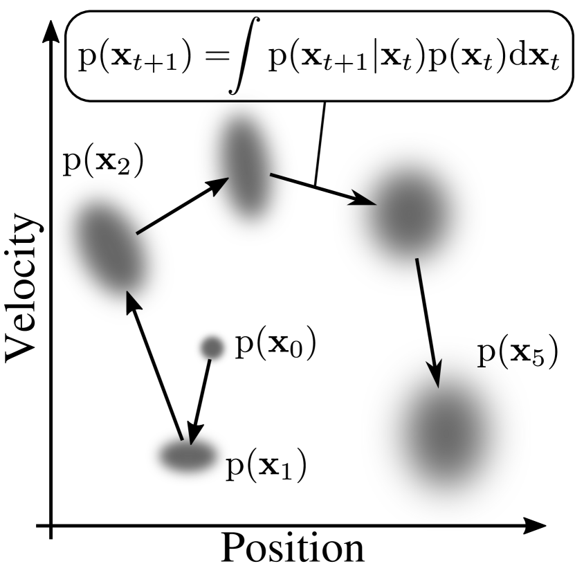
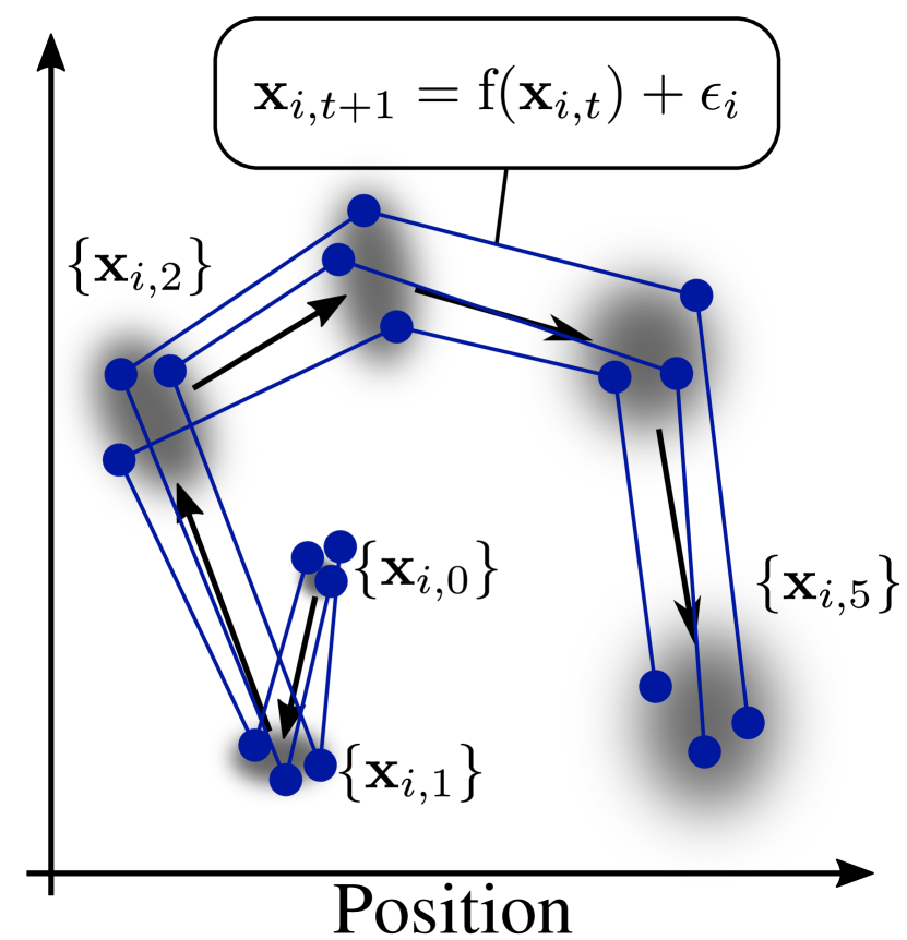
We were motivated by Probabilistic Inference for Learning Control (PILCO) (Deisenroth & Rasmussen, 2011), a model-based reinforcement learning (RL) algorithm which showed impressive results by learning continuous control tasks using several orders of magnitude less data than model-free alternatives. The keys to its success were a principled approach to model uncertainty, and analytic moment-matching (MM) based Gaussian approximations of trajectory distributions.

Unfortunately the MM framework is computationally inflexible. For example, it cannot be used with neural network models. Thus, this work searches for an alternative flexible method for evaluating trajectory distributions and gradients.

Particle sampling methods are a general scheme, which can be applied in practically any setting. Indeed, model-free algorithms have previously been successfully used with particle trajectories from the same types of models as used in PILCO (Kupcsik et al., 2014), (Chatzilygeroudis et al., 2017). Aiming for better performance, model-based gradients can be evaluated using the reparameterization (RP) trick to differentiate through stochasticities. This approach was previously attempted in the context of PILCO, but surprisingly, it did not work, with the poor performance attributed to local minima (McHutchon, 2014).

Recently, several works have attempted a similar method using Bayesian neural network dynamics models and the RP trick. Depeweg et al. (2016) successfully used this approach to solve non-standard problems. Gal et al. (2016), on the other hand, found that the direct approach with RP did not work on the standard cart-pole swing-up task. It is difficult to compare the new approaches to PILCO, because they simultaneously change multiple aspects of the algorithm: they switch the model to a more expressive one, then modify the policy search framework to accommodate this change. In our work, we perform a shorter step – we keep everything about PILCO the same, only changing the framework used for prediction. This approach allows better explaining how MM helps with learning. We find that reducing local minima was in fact not the main reason for its success over particle-based methods. The primary issue was a hopelessly large gradient variance when using particles and the RP trick.

We show that the large variance is due to chaos-like sensitive dependence on initial conditions – a common property in calculations involving long chains of nonlinear mappings. We refer to this problem as ”the curse of chaos”. Our work suggests that RP gradients and backpropagation alone are not enough. One either needs methods to prevent the curse from occurring, or other types of gradient estimators.

We derive new flexbile gradient estimators, which combine model-based gradients with the likelihood ratio (LR) trick (Glynn, 1990), also called REINFORCE (Williams, 1992) or the score function estimator. Our use of LR differs from the typical use in model-free RL – instead of sampling with a stochastic policy in the action space, we use a deterministic policy, but sample with a stochastic model in the state space. We also develop an importance sampling scheme for use within a batch of particles. Our estimators obtain accurate gradients, and allow surpassing the performance of PILCO.

Our results – LR gradients perform better than RP with backpropagation – are contradictory to recent work in stochastic variational inference, which suggest that even a single sample point yields a good gradient estimate using the RP trick (Kingma & Welling, 2014; Rezende et al., 2014; Ruiz et al., 2016). In our work, not only is a single sample not enough, even millions of particles would not suffice! In contrast, our new estimators achieve accurate gradients with a few hundred particles. As LR gradients are also not perfect, we further invent the total propagation algorithm, which efficiently combines the best of LR and RP gradients.

2 Background

2.1 Episodic Policy Search

For a review of policy search methods, see (Deisenroth et al., 2013). Consider discrete time systems described by a state vector ${\bf x}_{t}$ (the position and velocity of a robot) and the applied action/control vector ${\bf u}_{t}$ (the motor torques). An episode starts by sampling a state from a fixed initial state distribution ${\bf x}_{0}\sim p({\bf x}_{0})$. The policy $\pi_{\theta}$ determines what action is applied ${\bf u}_{t}\sim p({\bf u}_{t})=\pi({\bf x}_{t};\theta)$. Having applied an action, the state transitions according to an unknown dynamics function ${\bf x}_{t+1}\sim p({\bf x_{t+1}})=f({\bf x}_{t},{\bf u}_{t})$. Both the policy and the dynamics may be stochastic and nonlinear. Actions and state transitions are repeated for up to $T$ time-steps, producing a trajectory $\tau$: $({\bf x}_{0},{\bf u}_{0},{\bf x}_{1},{\bf u}_{1},...,{\bf x}_{T})$. Each episode is scored according to the return function $G(\tau)$. Often, the return decomposes into a sum of costs for each time step $G(\tau)=\sum_{t=0}^{T}c({\bf x}_{t})$, where $c({\bf x})$ is the cost function. The goal is to optimize the policy parameters $\theta$ to minimize the expected return $J(\theta)=\mathbb{E}_{\tau\sim p(\tau;\theta)}\left[G(\tau)\right]$. We define the value $V_{h}({\bf x})=\mathbb{E}\left[\sum_{t=h}^{T}c({\bf x}_{t})\right]$.

Learning alternates between executing the policy on the system, then updating $\theta$ to improve the performance on the following attempts. Policy gradient methods directly estimate the gradient of the objective function $\frac{\text{d}~{}}{\text{d}\theta}J(\theta)$ and use it for optimization. Some model-based policy search methods use all of the data to learn a model of $f$ denoted by $\hat{f}$, and use it for ”mental rehearsal” between trials to optimize the policy. Hundreds of simulated trials can be performed per real trial, greatly increasing data-efficiency. We utilize the fact that $\hat{f}$ is differentiable to obtain better gradient estimators over model-free algorithms. Importantly, our models are probabilistic, and predict state distributions.

2.2 Stochastic Gradient Estimation

Here we explain methods to compute the gradient of the expectation of an arbitrary function $\phi(x)$ with respect to the parameters of the sampling distribution $\frac{\text{d}~{}}{\text{d}\theta}\mathbb{E}_{x\sim p(x;\theta)}\left[\phi(x)\right]$, e.g. the expected return w.r.t. the policy parameters.

Reparameterization gradient (RP): Consider sampling from a univariate Gaussian distribution. One approach first samples with zero mean and unit variance $\epsilon\sim\mathcal{N}(0,1)$, then maps this point to replicate a sample from the desired distribution $x=\mu+\sigma\epsilon$. Now it is straight-forward to differentiate the output w.r.t. the distribution parameters, namely $\frac{\text{d}x}{\text{d}\mu}=1$ and $\frac{\text{d}x}{\text{d}\sigma}=\epsilon$. Averaging samples of $\frac{\text{d}\phi}{\text{d}x}\frac{\text{d}x}{\text{d}\theta}$ gives an unbiased estimate of the gradient of the expectation. This is the RP gradient for a normal distribution. For a multivariate Gaussian, the Cholesky factor ($L,\text{s.t.}\Sigma=LL^{T}$) of the covariance matrix can be used instead of $\sigma$. See (Rezende et al., 2014) for non-Gaussian distributions.

Likelihood ratio gradient (LR): The desired gradient can be written as $\frac{\text{d}~{}}{\text{d}\theta}\mathbb{E}_{x\sim p(x;\theta)}\left[\phi(x)\right]=\int\frac{\text{d}p(x;\theta)}{\text{d}\theta}\phi(x)\text{d}x$. In general, any function can be integrated by sampling from a distribution $q(x)$ by performing $\int\phi(x)\text{d}x=\int q(x)\frac{\phi(x)}{q(x)}\text{d}x=\mathbb{E}_{x\sim q}\left[\frac{\phi(x)}{q(x)}\right]$. The likelihood ratio gradient picks $q(x)=p(x)$, and directly integrates:

$$\int\frac{\text{d}p(x;\theta)}{\text{d}\theta}\phi(x)\text{d}x =\mathbb{E}_{x\sim p}\left[\frac{\frac{\text{d}p(x;\theta)}{\text{d}\theta}}{p(x)}\phi(x)\right]$$

$$=\mathbb{E}_{x\sim p}\left[\frac{\text{d}\log p(x;\theta)}{\text{d}\theta}\phi(x)\right]$$

The LR gradient often has a high variance, and has to be combined with variance reduction techniques known as control variates (Greensmith et al., 2004). A common approach subtracts a constant baseline $b$ from the function values to obtain the estimator $\mathbb{E}_{x\sim p}\left[\frac{\text{d}~{}}{\text{d}\theta}\left(\log p(x;\theta)\right)(\phi(x)-b)\right]$. If $b$ is independent from the samples, this can greatly reduce the variance without introducing any bias. In practice, the sample mean is a good choice $b=\mathbb{E}\left[\phi(x)\right]$. When estimating the gradient from a batch, one can estimate leave-one-out baselines for each point to obtain an unbiased gradient estimator (Mnih & Rezende, 2016), i.e. $b_{i}=\sum_{j\neq i}^{P}\phi(x_{j})/(P-1)$.

2.3 Trajectory Gradient Estimation

The probability density $p(\tau)=p({\bf x}_{0},{\bf u}_{0},{\bf x}_{1},{\bf u}_{1},...,{\bf x}_{T})$ of observing a particular trajectory can be written as $p({\bf x}_{0})\pi({\bf u}_{0}|{\bf x}_{0})p({\bf x}_{1}|{\bf x}_{0},{\bf u}_{0})...p({\bf x}_{T}|{\bf x}_{T-1},{\bf u}_{T-1})$.

To use RP gradients, one must know or estimate the dynamics $p({\bf x}_{t+1}|{\bf x}_{t},{\bf u}_{t})$ – in other words, RP is not applicable to the model-free case. With a model, a predicted trajectory can be differentiated by using the chain rule.

To use LR gradients, note that $p(\tau)$ is a product, so $\log p(\tau)$ can be transformed into a sum. Denote $G_{h}(\tau)=\sum_{t=h}^{T}c({\bf x}_{t})$. Noting that (1) only the action distributions depend on the policy parameters, and (2) an action does not affect costs obtained at previous time steps leads to the gradient estimator: $\mathbb{E}\left[\sum_{t=0}^{T-1}\left(\frac{\text{d}~{}}{\text{d}\theta}\log\pi({\bf u}_{t}|{\bf x}_{t};\theta)G_{t+1}(\tau)\right)\right]$

Algorithm 1 Analytic moment matching based trajectory prediction and policy evaluation (used in PILCO)

  Input: policy $\pi$ with parameters $\theta$, episode length $T$, initial Gaussian state distribution $p({\bf x}_{0})$, cost function $c({\bf x})$, learned dynamics model $\hat{f}$.

  Requirements: if the input distribution is Gaussian, can analytically compute the expectations and variances of the outputs of $\pi({\bf x})$, $\hat{f}({\bf x},{\bf u})$, $c({\bf x})$, and differentiate them.

  for $t=0$ to $T-1$ do

     1. Using $p({\bf x}_{t})$ and $\pi$ compute a Gaussian approximation to the joint state-action distribution:

         $p({\bf\tilde{x}}_{t})=\mathcal{N}(\tilde{\mu}_{t},\tilde{\Sigma}_{t})$, where ${\bf\tilde{x}}_{t}=[x^{T}_{t},u^{T}_{t}]^{T}$

     2. Using $p({\bf\tilde{x}}_{t})$ and $\hat{f}$ compute a Gaussian approximation to the next state distribution:

         $p({\bf x}_{t+1})=\mathcal{N}(\mu_{t+1},\Sigma_{t+1})$

     3. Using $p({\bf x}_{t+1})$ and $c({\bf x})$ compute the expected cost:

         $\mathbb{E}\left[c({\bf x}_{t+1})\right]$

  end for

  Gradient computation: $\frac{\text{d}~{}}{\text{d}\theta}\left(\sum_{t=1}^{T}\mathbb{E}\left[c({\bf x}_{t})\right]\right)$ is computed analytically during the for-loop by differentiating each computation separately and applying the chain rule.

2.4 PILCO

The higher level view of PILCO follows Section 2.1 and the policy gradient evaluation is detailed in Algorithm 1.

2.4.1 Probabilistic Dynamics Model

We follow the original PILCO, which uses Gaussian process (Rasmussen & Williams, 2006) dynamics models to predict the change in state from one time step to the next, i.e. $p(\Delta x_{t+1}^{a})=\mathcal{GP}({\bf x}_{t},{\bf u}_{t})$, where ${\bf x}\in\mathbb{R}^{D}$, ${\bf u}\in\mathbb{R}^{F}$ and $\Delta x_{t+1}^{a}=x_{t+1}^{a}-x_{t}^{a}$. A separate Gaussian process is learned for each dimension $a$. We use a squared exponential covariance function $k_{a}({\bf\tilde{x}},{\bf\tilde{x}^{\prime}})=s_{a}^{2}\exp(-({\bf\tilde{x}}-{\bf\tilde{x}^{\prime}})^{T}\Lambda_{a}^{-1}({\bf\tilde{x}}-{\bf\tilde{x}^{\prime}}))$, where $s_{a}$ and $\Lambda=\text{diag}([l_{a1},l_{a2},...,l_{a{D+F}}])$ are the function variance and length scale hyperparameters respectively. We use a Gaussian likelihood function with a noise hyperparameter $\sigma_{n}$. The hyperparameters are trained to maximize the marginal likelihood. When sampling from these models, the prediction has the form $y=\hat{f}({\bf x})+\epsilon$, where $\epsilon\sim\mathcal{N}\left(0,\sigma_{f}^{2}({\bf x})+\sigma_{n}^{2}\right)$. Here $\sigma_{f}^{2}$ represents the model uncertainty, and is caused by a lack of data in a region, while $\sigma_{n}^{2}$ is the learned inherent model noise. The learned model noise is not necessarily the same as the real observation noise $\sigma_{o}^{2}$ in the system. In particular, the latent state is not modeled and the system is approximated by predicting the next observation given the current observation. Moreover, there is an additional source of the variance in the trajectory – with different start locations, the trajectory will differ.

2.4.2 Moment matching Prediction

In general, when a Gaussian distribution is mapped through a nonlinear function, the output is intractable and non-Gaussian; however, in some cases one can analytically evaluate the moments of the output distribution. Moment-matching (MM) approximates the output distribution as Gaussian by matching the mean and variance with the true moments. Note that even though the state-dimensions are modelled with separate functions $\hat{f}_{a}$, MM is performed jointly, and the state distributions can include covariances.

3 Particle Model-Based Policy Search

3.1 Particle Prediction

In general, particle trajectory predictions are simple – predict at all particle locations, sample from the output distributions, repeat. However, we also compare to a scheme based on Gaussian resampling (GR), used by Gal et al. (2016) to apply PILCO with neural network dynamics models.

Gaussian resampling (GR): MM can be stochastically replicated. At each time step, the mean $\hat{\mu}=\sum_{i=1}^{P}{\bf x}_{i}/P$ and covariance $\hat{\Sigma}=\sum_{i=1}^{P}({\bf x}_{i}-\hat{\mu})({\bf x}_{i}-\hat{\mu})^{T}/(P-1)$ of the particles are estimated. Then the particles are resampled from the fitted distribution $x^{\prime}_{i}\sim\hat{\mu}+L{\bf z}_{i}~{}|~{}{\bf z}_{i}\sim\mathcal{N}(0,I)$, where $L$ is the Cholesky factor of $\hat{\Sigma}$. One can differentiate this resampling operation by using RP. Obtaining the gradient $\text{d}{L}/\text{d}{\hat{\Sigma}}$ is non-trivial, but (Murray, 2016) presents an overview. We use the provided symbolic expression.

3.2 Hybrid Gradient Estimation Techniques

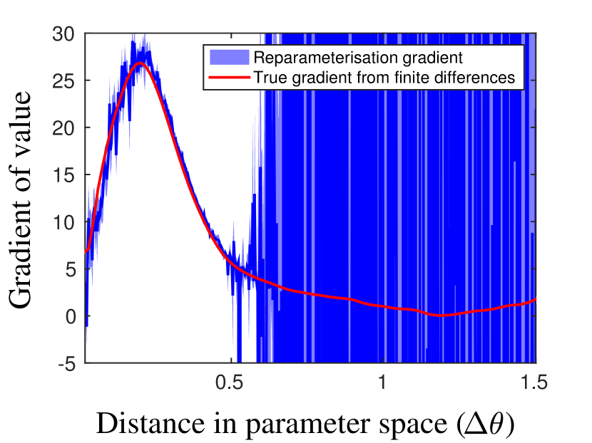
In our case, RP gradients can be used. However, surprisingly they were hopelessly inaccurate (see Figure 2(d)). To solve the problem, we derived new gradient estimators which combine model derivatives with LR gradients. In particular, our approach allowed for within batch importance sampling to increase sample efficiency.

Model-based LR: As in Section 2.3, one can write the distribution over predicted trajectories as $p(\tau)=p({\bf x}_{0})\pi({\bf u}_{0}|{\bf x}_{0})\hat{f}({\bf x}_{1}|{\bf x}_{0},{\bf u}_{0})...\hat{f}({\bf x}_{T}|{\bf x}_{T-1},{\bf u}_{T-1})$. With deterministic policies, the model and policy can be combined: $p({\bf x}_{t+1}|{\bf x}_{t})=\hat{f}({\bf x}_{t+1}|{\bf x}_{t},\pi({\bf x}_{t};\theta))$, which is differentiable $\frac{\text{d}p_{t+1}}{\text{d}\theta}=\frac{\text{d}p_{t+1}}{\text{d}{\bf u}_{t}}\frac{\text{d}{\bf u}_{t}}{\text{d}\theta}$. A model-based gradient derives: $\mathbb{E}\left[\sum_{t=0}^{T-1}\left(\frac{\text{d}~{}}{\text{d}\theta}\log p({\bf x}_{t+1}|{\bf x}_{t};\theta)(G_{t+1}({\bf x}_{t+1})-b_{t+1})\right)\right]$

Batch Importance Weighted LR (BIW-LR): We use parallel computation, and sample multiple particles simultaneously. The state distribution is represented as a mixture distribution $q({\bf x}_{t+1})=\sum_{i=1}^{P}p({\bf x}_{t+1}|{\bf x}_{i,t};\theta)/P$. Analogously to the derivation of LR in Section 2.2, one can derive a lower variance estimator with importance sampling within the batch for each time step: $\sum_{i=1}^{P}\sum_{j=1}^{P}\left(\frac{\text{d}{p({\bf x}_{j,t+1}|{\bf x}_{i,t};\theta)}/\text{d}{\theta}}{\sum_{k=1}^{P}p({\bf x}_{j,t+1}|{\bf x}_{k,t})}(G_{t+1}({\bf x}_{j,t+1})-b_{i,t+1})\right)/P$

We choose to estimate a leave-one-out mean of the returns by normalized importance sampling with the equation: $b_{i,t+1}=\left(\sum_{j\neq i}^{P}c_{j,t+1}G_{t+1}({\bf x}_{j,t+1})\right)/\sum_{j\neq i}^{P}c_{j,t+1}$, where $c_{j,t+1}=p({\bf x}_{j,t+1}|{\bf x}_{i,t})/\sum_{k=1}^{P}p({\bf x}_{j,t+1}|{\bf x}_{k,t})$. Without normalizing, a large variance of the baseline estimation leads to poor LR gradients. Note that we compute $P$ baselines for each time-step, whereas there are $P^{2}$ components in the gradient estimator. To obtain a true unbiased gradient, one should compute $P^{2}$ leave-one-out baselines – one for each particle for each mixture component of the distribution. The paper contains evaluations only with the baseline presented here – we found that it already removes most of the bias.

Algorithm 2 Total Propagation Algorithm
(used in PIPPS for evaluating the gradient)

  This algorithm provides an efficient method to fuse LR and RP gradients by combining ideas from filtering and back-propagation. The algorithm is explained here with reference to our policy search framework.

  Forward pass: Compute a set of particle trajectories.

  Backward pass:

  Initialise: $\frac{\text{d}G_{T+1}}{\text{d}\zeta_{T+1}}={\bf 0}$, $\frac{\text{d}J}{\text{d}\theta}={\bf 0}$, $G_{T+1}=0$ where $\zeta$ are the distribution parameters, e.g. $\mu$ and $\sigma$.

  for $t=T$ to $1$ do

     for each particle $i$ do

        $G_{i,t}=G_{i,t+1}+c_{i,t}$, where $c_{t}$ is the cost at time t.

        $\frac{\text{d}{\bf\zeta}_{i,t+1}}{\text{d}{\bf x}_{i,t}}=\frac{\partial{\bf\zeta}_{i,t+1}}{\partial{\bf x}_{i,t}}+\frac{\text{d}{\bf\zeta}_{i,t+1}}{\text{d}{\bf u}_{i,t}}\frac{\text{d}{\bf u}_{i,t}}{\text{d}{\bf x}_{i,t}}$

        $\frac{\text{d}G_{i,t}^{RP}}{\text{d}\zeta_{i,t}}=(\frac{\text{d}G_{i,t+1}}{\text{d}\zeta_{i,t+1}}\frac{\text{d}\zeta_{i,t+1}}{\text{d}{\bf x}_{i,t}}+\frac{\text{d}c_{i,t}}{\text{d}{\bf x}_{i,t}})\frac{\text{d}{\bf x}_{i,t}}{\text{d}\zeta_{i,t}}$

        $\frac{\text{d}G_{i,t}^{LR}}{\text{d}\zeta_{i,t}}=(G_{i,t}-b_{i,t})\frac{\text{d}\log p({\bf x}_{i,t})}{\text{d}\zeta_{i,t}}$

        $\frac{\text{d}G_{i,t}^{RP}}{\text{d}\theta}=\frac{\text{d}G_{i,t}^{RP}}{\text{d}\zeta_{i,t}}\frac{\text{d}\zeta_{i,t}}{\text{d}{\bf u}_{i,t-1}}\frac{\text{d}{\bf u}_{i,t-1}}{\text{d}\theta}$

        $\frac{\text{d}G_{i,t}^{LR}}{\text{d}\theta}=\frac{\text{d}G_{i,t}^{LR}}{\text{d}\zeta_{i,t}}\frac{\text{d}\zeta_{i,t}}{\text{d}{\bf u}_{i,t-1}}\frac{\text{d}{\bf u}_{i,t-1}}{\text{d}\theta}$

     end for

     $\sigma^{2}_{RP}=\text{trace}(\mathbb{V}\left[\frac{\text{d}G_{i,t}^{RP}}{\text{d}\theta}\right])$, $\sigma^{2}_{LR}=\text{trace}(\mathbb{V}\left[\frac{\text{d}G_{i,t}^{LR}}{\text{d}\theta}\right])$

     $k_{LR}=1/\left(1+\frac{\sigma^{2}_{LR}}{\sigma^{2}_{RP}}\right)$

     $\frac{\text{d}J}{\text{d}\theta}=\frac{\text{d}J}{\text{d}\theta}+k_{LR}\frac{1}{P}\sum_{i}^{P}\frac{\text{d}G_{i,t}^{LR}}{\text{d}\theta}+(1-k_{LR})\frac{1}{P}\sum_{i}^{P}\frac{\text{d}G_{i,t}^{RP}}{\text{d}\theta}$

     for each particle $i$ do

        $\frac{\text{d}G_{i,t}}{\text{d}\zeta_{i,t}}=k_{LR}\frac{\text{d}G_{i,t}^{LR}}{\text{d}\zeta_{i,t}}+(1-k_{LR})\frac{\text{d}G_{i,t}^{RP}}{\text{d}\zeta_{i,t}}$

     end for

  end for

RP/LR weighted average: The bulk of the computation is spent on the $\text{d}p({\bf x}_{t+1}|{\bf x_{t}};\theta)/\text{d}\theta$ terms. These terms are needed for both LR and RP gradients, so there is no penalty to combining both estimators. A well known statistics result states that for independent estimators, an optimal weighted average estimate is achieved if the weights are proportional to the inverse variance, i.e. $\mu=\mu_{LR}k_{LR}+\mu_{RP}k_{RP}$, where $k_{LR}=\hat{\sigma}_{LR}^{-2}/(\hat{\sigma}_{LR}^{-2}+\hat{\sigma}_{RP}^{-2})$ and $k_{RP}=1-k_{LR}$.

A naive combination scheme would compute the gradient separately for the whole trajectory for both estimators, then combine them; however, this approach neglects the opportunity to use reparameterization gradients through shorter sections of the trajectory to obtain better gradient estimates. Our new total propagation algorithm (TP) goes beyond the naive method. TP uses a single backward pass to compute a union over all possible RP depths, automatically giving greater weight to estimators with lower variance.

A description is provided in Algorithm 2. At each backward step, it evaluates the gradient w.r.t. the policy parameters using both the LR and RP methods. It evaluates a ratio based on the variances in policy parameter space – this variance is proportional to the variance of the policy gradient estimator. The gradients are combined, and a ”best” estimate in distribution parameter space is passed to the previous time step. In the algorithm, the $\mathbb{V}$ operator takes the sample variance of gradient estimates from different particles; however, other variance estimation schemes could also be considered: one could estimate variances from moving averages of the magnitude of the gradient, use a different statistical estimator for the variance, use only a subset of policy parameters, etc. The algorithm is not limited to RL problems, but is applicable to general stochastic computation graphs (Schulman et al., 2015), and could be used for training probabilistic models, stochastic neural networks, etc.

3.3 Policy Optimization

RMSprop-like stochastic gradient descent: We use an algorithm motivated by RMSprop (Tieleman & Hinton, 2012). RMSprop normalizes its SGD steps by utilizing a running average of the square of the gradients. In our case, since our batch sizes were large, we directly estimate the expectation of the square from the batch by $z=\mathbb{E}\left[g^{2}\right]=\mathbb{E}\left[g\right]^{2}+\mathbb{V}\left[g\right]$, where $g$ is the gradient. We use the variance of the mean, i.e. $\mathbb{V}\left[g\right]$ is the variance divided by the number of particles $P$. The gradient step becomes $g/\sqrt{z}$. We use momentum with the parameter $\gamma$. The full update equations become:

$$m \leftarrow\gamma m+g/\sqrt{\mathbb{E}\left[g\right]^{2}+\mathbb{V}\left[g\right]}$$

$$\theta \leftarrow\theta-\alpha m$$

Deterministic optimizer: The random number seed can be fixed to turn a stochastic problem deterministic, also known as the PEGASUS trick (Ng & Jordan, 2000). With a fixed seed, the RP gradient is an exact gradient of the objective, and quasi-Newton optimizers, such as BFGS can be used.

4 Experiments

We performed experiments with two purposes: 1. To explain why RP gradients are not sufficient (Section 4.1). 2. To show that our newly developed methods can match up to PILCO in terms of learning efficiency (Section 4.2).

4.1 Plotting the Value Landscape

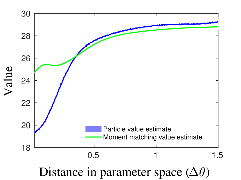
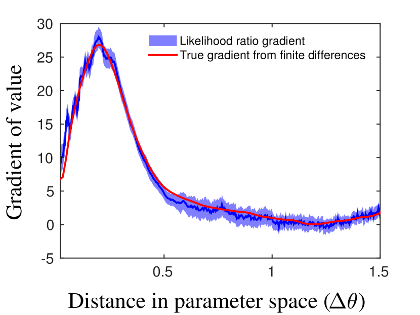
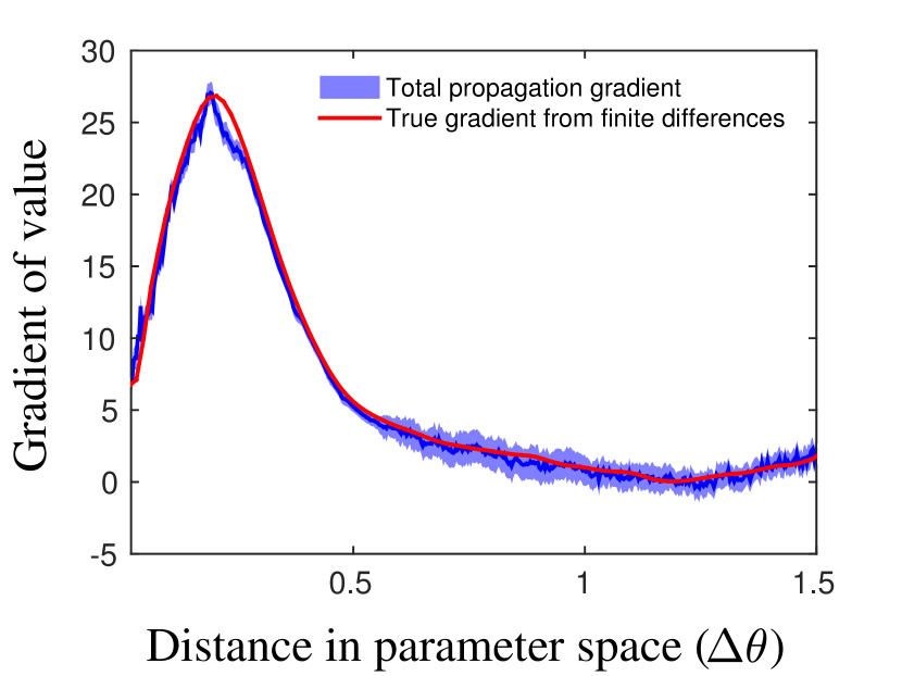
We perturb the policy parameters $\theta$ in a randomly chosen fixed direction, and plot both the objective function, and the magnitude of the projected gradient as a function of $\Delta\theta$. The results of this experiment are perhaps the most striking component of our paper, and motivated the term ”the curse of chaos”. Refer to Figure 2 for the results, and to Section 4.1.1 for a full explanation.

The plots were generated in the nonlinear cart-pole task, using similar settings as explained in Section 4.2. We used 1000 particles, and while keeping the random number seed fixed to demonstrate that the high variance in 2(d) is not caused by randomness, but by a chaos-like property of the system. The confidence intervals were estimated by $Var/P$ where $Var$ is the sample variance, and $P$ is the number of particles. In Section 4.1.2 we plot the dependence of the variance on $P$ using a more principled approach.

4.1.1 Explaining the Curse of Chaos

(a)

(b) Value at $\text{p}({\bf x}_{1})$ and $\Delta\theta=0$

(c) Value at $\text{p}({\bf x}_{1})$ and $\Delta\theta=1.5$

(d) $\text{RP}_{\text{FS}}$ (Exact gradient of value in 2(a))

(e) LR

(f) TP

Figure 2: To illustrate the behavior of the gradient estimators in the cart-pole task, we fix the random number seed, vary the policy parameters $\theta$ in a fixed direction, and plot a 95% confidence interval for both the objective (2(a)) and the magnitude of the gradient estimators in this direction (2(d),2(e),2(f)). Figure 2(d) shows that reparameterization gradients suffer from the curse of chaos, which can cause the gradient variance to explode. Our new estimators in Figures 2(e) and 2(f) are robust to this issue. Figures 2(b) and 2(c) correspond to the parameter settings at the left and right side of the other plots, and explain the reason for the exploding gradient variance. Refer to Section 4.1.1 for a full explanation. The confidence interval of the particle value estimate in (2(a)) is so tight, that the line is thicker, but note that a smooth line would fit within the error bounds. Moreover, note that having fixed the random number seed causes a bias.

Figure 2(d) contains a peculiar result where the RP gradient behaves well for some regions of the parameters $\theta$, but when $\theta$ is perturbed, a phase-transition-like change causes the variance to explode. The variance at $\Delta\theta=1.5$ is $\sim$$4\times 10^{5}$ times larger than at $\Delta\theta=0$, meaning that $\sim$$4\times 10^{8}$ particles would be necessary for the RP gradient to become accurate in that region. For practical purposes, optimizing with the RP gradient would lead to a simple random walk.

Since the seed was fixed, the RP gradient in 2(d) is an exact gradient of the value in 2(a). Therefore, there is an infinitesimal deterministic ”noise” at the right of 2(a). The value averaged across 1000 particles is though not the true objective – that would require averaging an infinite number of particles. When averaging an infinite amount of particles, is there still a ”noise”, or does the function become smooth?

Our new gradient estimators in Figures 2(e) and 2(f) suggest that the true objective is indeed smooth. To provide more evidence, we estimated the magnitude of the gradient from finite differences of the value in 2(a) using a sufficiently large perturbation in $\theta$, such that the ”noise” is ignored. The fact that two separate approaches agree – one which varies the policy parameters $\theta$, and another which keeps $\theta$ fixed, but estimates the gradient from the trajectories – provides convincing evidence that the true objective is smooth.

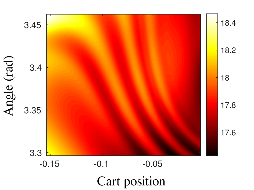
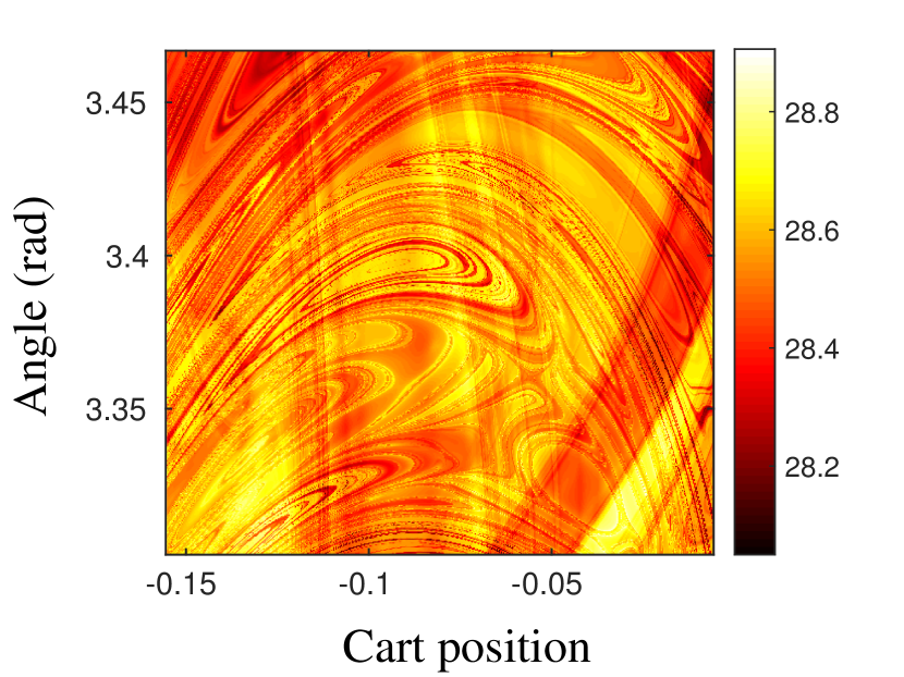
Figures 2(b) and 2(c) explain the reason for the explosion of the variance when using RP gradients (2(d)). Figure 2(b) corresponds to the leftmost parameter setting ($\Delta\theta=0$); Figure 2(c) corresponds to the rightmost parameter setting ($\Delta\theta=1.5$). The plots show how the value $V({\bf x};\theta)$ (the remaining cumulative cost) varies as a function of the state position ${\bf x}$. Note that because the random number seed is fixed, the value $V$ is the same as the remaining return $G$. This definition differs from the typical value function, which averages the return over an infinite amount of particles. The figures were created by predicting the trajectory at each point for 4 particles with different fixed seeds, then averaging the costs of the trajectories. We chose to predict 4 particles after trying 1 particle, for which the value appeared to include a step-like part, but was otherwise less interesting than the current figure. As the average value of the 4 particles is erratic, at least one of the 4 particles must have a highly erratic value in the shown region.

The boxes (2(b), 2(c)) are centered at the mean prediction from the center of the initial state distribution (if unclear, consider Figure 1 with $p({\bf x}_{0})$ as a point mass, then $p({\bf x}_{1})$ depicts the location of the box). The axes on the boxes are slightly different, because when $\theta$ is changed, the predicted location $p({\bf x}_{1};\theta)$ changes. The side lengths correspond to 4 standard deviations of the Gaussian distributions $p({\bf x}_{1};\theta)$. The velocities were kept fixed at the mean values.

RP estimates $\frac{\text{d}}{\text{d}\theta}\int p({\bf x}_{1};\theta)V({\bf x}_{1})\text{d}{\bf x}$. It samples points inside the box, computes the gradient $\frac{\partial V}{\partial\theta}=\frac{\partial V}{\partial x}\frac{\text{d}x}{\text{d}\theta}$ and averages the samples together. In Figure 2(c) finding the gradient of the expectation by differentiating $V$ is completely hopeless. In contrast, the LR gradient (2(e)) only uses the value $V$, not its derivative, and does not suffer from this problem.

Finally, even though we do not show the plotted value and gradient for the Gaussian resampling case, both of these were smooth functions for a fixed random seed. Thus, resampling also beats the curse of chaos.

4.1.2 Policy Gradient Variance Evaluation

(a) $\Delta\theta=0$

(b) $\Delta\theta=1.5$

Figure 3: Computed variances corresponding to plots in Figure 2.

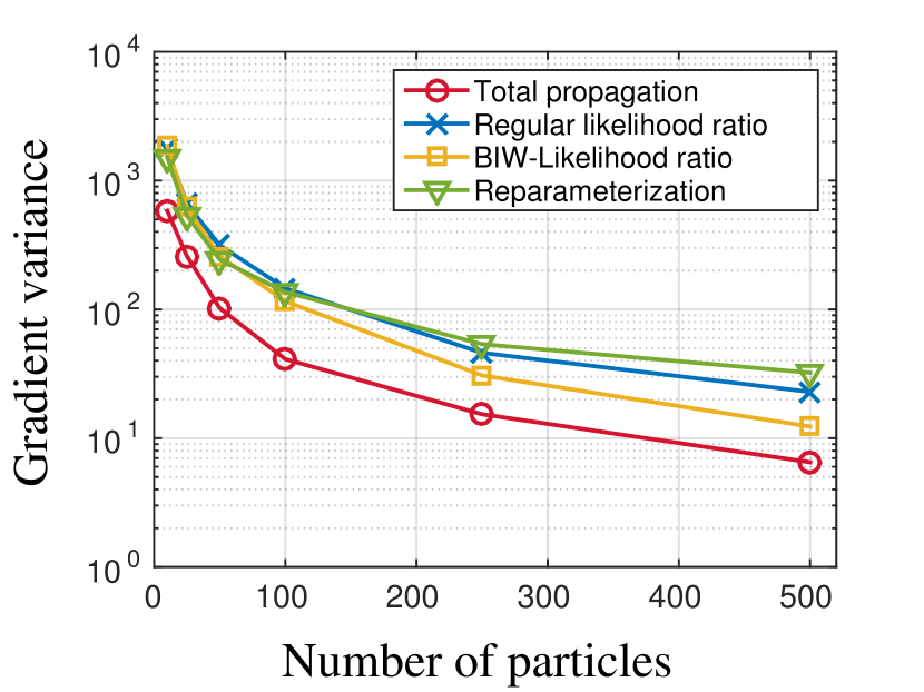
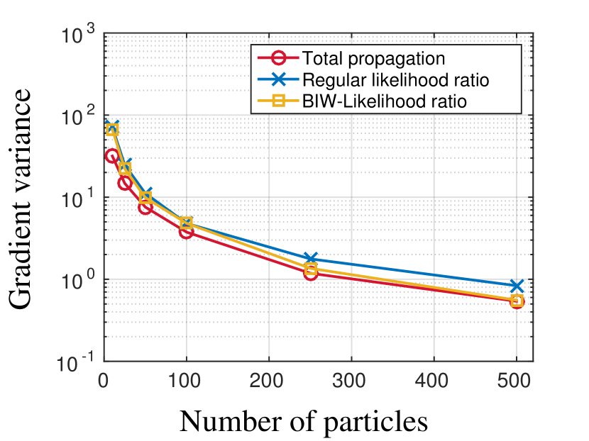
In Figure 3, we plot how the variance of the gradient estimators at $\Delta\theta=0$ and $\Delta\theta=1.5$ depends on the number of particles $P$. The variance was computed by repeatedly sampling the estimator for a large number of times and calculating the variance from the set of evaluations. We compare RP, TP as well as LR gradients both with and without batch importance weighting (BIW) to show that our importance sampling scheme reduces the variance. We used the importance sampled baseline; in practice the regular LR gradient would use a simpler baseline, and have even higher variance. The RP gradient is omitted from 3(b), because the variance was between $10^{8}$-$10^{15}$. The TP gradient combined the BIW-LR and RP gradients.

The results confirm that BIW significantly reduces the variance. Moreover, our TP algorithm was the best. Importantly, in 3(b), even though the variance of the RP gradient for the full trajectory is over $10^{6}$ larger than the other estimators, TP utilizes shorter path-length RP gradients to obtain 10-50% reduction in variance for 250 particles and fewer.

4.2 Learning Experiments

We compare PILCO in episodic learning tasks to the following particle-based methods: RP, RP with a fixed seed (RP${}_{\text{FS}}$), Gaussian resampling (GR), GR with a fixed seed (GR${}_{\text{FS}}$), model-based batch importance weighted likelihood ratio (LR) and total propagation (TP). Moreover, we evaluate two variations of the particle predictions: 1. TP while ignoring model uncertainty, and adding only the noise at each time step ($\text{TP}-\sigma_{f}$). 2. TP with increased prediction noise ($\text{TP}+\sigma_{n}$). We used 300 particles in all cases.

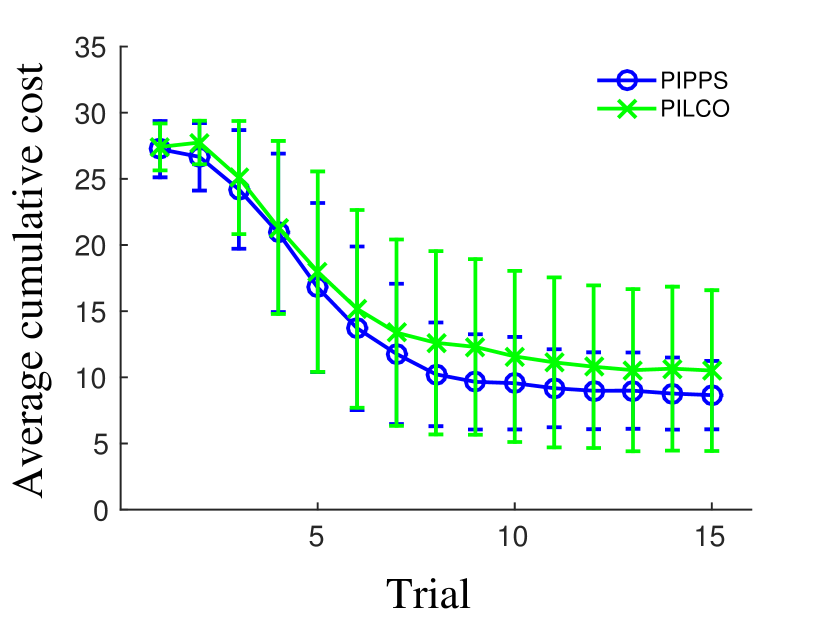
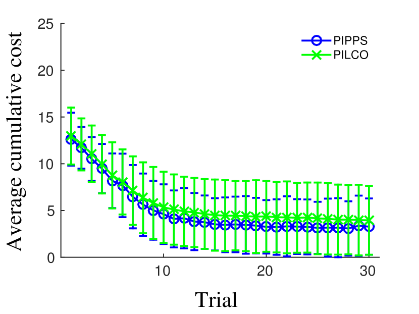
We performed learning tasks from a recent PILCO paper (Deisenroth et al., 2015): cart-pole swing-up and balancing, and unicycle balancing. The simulation dynamics were set to be the same, and other aspects were similar to the original PILCO. The results are in Tables 2 and 1, and in Figure 4.

Common properties in the tasks: The optimizer was run for 600 policy evaluations between each trial. The SGD learning rate, and momentum parameters were $\alpha=5\times 10^{-4}$ and $\gamma=0.9$. The episode lengths were 3s for the cart-pole, and 2s for the unicycle. Note that for the unicycle task, 2s was not sufficient for the policy to generalize to long trials, but it still allowed comparing to PILCO. The control frequencies were 10Hz. The costs were of the type $1-\exp(-({\bf x}-{\bf t})^{T}Q({\bf x}-{\bf t}))$, where ${\bf t}$ is the target. The outputs from the policies $\pi({\bf x})$ were constrained by a saturation function: $\text{sat}({\bf u})=9\sin({\bf u})/8+\sin(3{\bf u})/8$, where ${\bf u}=\tilde{\pi}({\bf x})$. One experiment consisted of (1; 5) random trials followed by (15; 30) learned trials for the cart and unicycle tasks respectively. Each experiment was repeated 100 times and averaged. Each trial was evaluated by running the policy 30 times, and averaging, though note that this was performed only for evaluation purposes – the algorithms only had access to 1 trial. Success was determined by whether the return of the final trial passed below a threshold.

4.2.1 Task Descriptions

Cart-pole Swing-up and Balancing: This is a standard control theory benchmark problem. The task consists of pushing a cart back and forth, to swing an attached pendulum to an upright position, then keep it balanced. The state space was represented as ${\bf x}=[s,\beta,\dot{s},\dot{\beta}]$, where $s$ is the cart-position and $\beta$ the pole angle. The base noise levels were $\sigma_{s}=0.01~{}\text{m},\sigma_{\beta}=1~{}\text{deg},\sigma_{\dot{s}}=0.1~{}\text{m/s},\sigma_{\dot{\beta}}=10~{}\text{deg/s}$. The noise was modified in different experiments by a multiplier $k$: $\sigma^{2}=k\sigma^{2}_{base}$. The original paper considered direct access to the true state. We set $k=10^{-2}$ to obtain a similar setting, but also tested $k\in\{1,4,9,16\}$. The policy $\tilde{\pi}$ was a radial basis function network (a sum of Gaussians) with 50 basis functions. We considered two cost functions. One was the same as in the original PILCO, with ${\bf x}$ including the sine and cosine, and depended on the distance between the tip of the pendulum to the position of the tip when the pendulum is balanced (Tip Cost). The other cost used the raw angle, and had $Q=\text{diag}([1,1,0,0])$ (Angle Cost). This cost differs conceptually from the Tip Cost, because there is only one correct direction in which to swing up the pendulum.

(a) Cart-pole

(b) Unicycle

Figure 4: PIPPS using TP matches PILCO in data-efficiency.

Table 1: Success rate of learning unicycle balancing

PILCO	RP	RP${}_{\text{FS}}$	GR	GR${}_{\text{FS}}$	LR	TP
0.91	0.80	0.39	0.96	0.63	0.47	0.94

Table 2: Success rate of learning cart-pole swing-up

Cost Function	Noise Multiplier	PILCO	RP	RP${}_{\text{FS}}$	GR	GR${}_{\text{FS}}$	LR	TP	TP$-\sigma_{f}$	TP$+\sigma_{n}$
Angle Cost	$k=10^{-2}$	0.88	0.69	0.24	0.63	0.74	0.57	0.82		0.96
Angle Cost	$k=1$	0.79	0.74	0.23	0.89	0.71	0.96	0.99	0.93
Angle Cost	$k=4$	0.70	0.58	0.08	0.62	0.41	0.94	0.95
Angle Cost	$k=9$	0.37	0.44	0.04	0.34	0.25	0.86	0.83
Angle Cost	$k=16$	0.01	0.11	0.00	0.08	0.02	0.45	0.40
Tip Cost	$k=10^{-2}$	0.92	0.44	0.20	0.47	0.78	0.36	0.54
Tip Cost	$k=1$	0.73	0.15	0.08	0.68	0.50	0.28	0.48

Unicycle balancing: See (Deisenroth et al., 2015) for a description. The task consists of balancing a unicycle robot, with state dimension $D=12$, and control dimension $F=2$. The noise was set to a low value. The controller $\tilde{\pi}$ is linear.

5 Discussion

5.1 Learning Experiments

PILCO performs well in scenarios with no noise, but with noise added the results deteriorate. This deterioration is most likely caused by an accumulation of errors in the MM approximations, previously observed by Vinogradska et al. (2016), who used quadrature for predictions. Particles do not suffer from this issue, and using TP gradients consistently outperforms PILCO with high noise.

On the other hand, at low noise levels, the performance of TP as well as LR reduces. If all of the particles are sampled from a small region, it becomes difficult to estimate the gradient from changes in the return – in the limit of a delta distribution an LR gradient could not even be evaluated. The TP gradient is less susceptible to this problem, because it incorporates information from RP. Finally, if the uncertainty in predictions is very low (as in $k=10^{-2}$), one can consider model noise as a parameter that affects learning, and increase it to acquire more accurate gradients: see $\text{TP}+\sigma_{n}$, where the model noise variance was multiplied by 100.

Notably, approaches which use MM, such as PILCO, and GR outperform the others when using the Tip Cost. The reason may be the multi-modality of the objective – with the Tip Cost, the pendulum may be swung up from either direction to solve the task; with the Angle Cost there is only one correct direction. Performing MM forces the algorithm along a unimodal path, whereas the particle approach could attempt a bimodal swing-up where some particles go from one side, and the rest from the other side. Thus, MM may be performing a kind of ”distributional reward shaping”, simplifying the optimization problem. Such an explanation was previously provided by Gal et al. (2016).

Finally, we point to the surprising $\text{TP}-\sigma_{f}$ experiment. Even though the predictions ignore model uncertainty, the method achieves 93% success rate. It is difficult to explain why learning still worked, but we hypothesize that the success may be related to the 0 prior mean of the GP. In regions where there is no data, the mean of the GP dynamics model goes to 0, meaning that the input control signal has no effect on the particle. Therefore, for the policy optimization to be successful, the particles would have to be controlled to stay in regions where there exists data. Note that a similar result was found by Chatzilygeroudis et al. (2017) who used an evolutionary algorithm and achieved 85-90% success rate at the cart-pole task even when ignoring model uncertainty.

5.2 The Curse of Chaos in Deep Learning

Most machine learning problems involve optimizing the expectation of an objective function $J({\bf x};\theta)$ over some data generating distribution $p_{Data}({\bf x})$, where this distribution can only be accessed through sample data points $\{{\bf x}_{i}\}$. Our predictive framework is analogous to a deep model: $p({\bf x}_{0})$ is the data generating distribution, $p({\bf x}_{t};\theta)$ are obtained by pushing $p_{Data}({\bf x})$ through the model layers. The most common method of optimization is SGD with pathwise derivatives computed by backpropagation. Our results suggest that in some situations – particularly with very deep or recurrent models – this approach could degenerate into a random walk due to an exploding gradient variance.

Exploding gradients have been observed in deep learning research for a long time (Doya, 1993; Bengio et al., 1994). Typically this phenomenon is regarded as a numerical issue, which leads to large steps and unstable learning. Common countermeasures include gradient clipping, ReLU activation functions (Nair & Hinton, 2010) and smart initializations. Our explanation to the problem is different: it is not just that the gradient becomes large, the gradient variance explodes, meaning that any sample from ${\bf x}_{i}\sim p_{Data}$ provides essentially no information about how to change the model parameters $\theta$ to increase the expectation of the objective over the whole distribution $\mathbb{E}_{p_{Data}}\left[J({\bf x})\right]$. While choosing a good initialization is an approach to tackle the problem, it appears difficult to guarantee that the system does not become chaotic during learning. For example, in econometrics there are even cases where the optimal policy may lead to chaotic dynamics (Deneckere & Pelikan, 1986). Gradient clipping can stop large parameter steps, but it will not fundamentally solve the problem if the gradients become random. Considering that chaos does not occur in linear systems (Alligood et al., 1996), our analysis suggests a reason for why piece-wise linear activations, which may be less susceptible to chaos, such as ReLUs perform well in deep learning.

While we have yet to computationally confirm our deep hypothesis, several works have investigated chaos in neural networks (Kolen & Pollack, 1991; Sompolinsky et al., 1988), although we believe we are the first to suggest that chaos may cause gradients to degenerate when computed using backpropagation. Notably, Poole et al. (2016) suggested that such properties lead to ”exponential expressivity”, but we believe that this phenomenon may instead be a curse.

6 Conclusions & Future Work

We may have described a limitation of optimizing expectations using pathwise derivatives, such as those computed by backpropagation. Moreover, we show a method to counteract this curse by injecting noise into computations, and using the likelihood ratio trick. Our total propagation algorithm provides an efficient method to combine reparameterization gradients on arbitrary stochastic computation graphs with any amount of other gradient estimators – even gradients computed using a value function could be used. There are countless ways to expand our work: better optimization, incorporate natural gradients, etc. The flexible nature of our method should make it easy to extend.

References

- Alligood et al. (1996) Alligood, K. T., Sauer, T. D., and Yorke, J. A. Chaos. Springer, 1996.
- Bengio et al. (1994) Bengio, Y., Simard, P., and Frasconi, P. Learning long-term dependencies with gradient descent is difficult. IEEE transactions on neural networks, 5(2):157–166, 1994.
- Chatzilygeroudis et al. (2017) Chatzilygeroudis, K., Rama, R., Kaushik, R., Goepp, D., Vassiliades, V., and Mouret, J.-B. Black-box data-efficient policy search for robotics. In Intelligent Robots and Systems (IROS), 2017 IEEE/RSJ International Conference on, pp. 51–58. IEEE, 2017.
- Deisenroth & Rasmussen (2011) Deisenroth, M. P. and Rasmussen, C. E. PILCO: A model-based and data-efficient approach to policy search. In International Conference on Machine Learning, pp. 465–472, 2011.
- Deisenroth et al. (2013) Deisenroth, M. P., Neumann, G., Peters, J., et al. A survey on policy search for robotics. Foundations and Trends in Robotics, 2(1-2):1–142, 2013.
- Deisenroth et al. (2015) Deisenroth, M. P., Fox, D., and Rasmussen, C. E. Gaussian processes for data-efficient learning in robotics and control. IEEE Transactions on Pattern Analysis and Machine Intelligence, 37(2):408–423, 2015.
- Deneckere & Pelikan (1986) Deneckere, R. and Pelikan, S. Competitive chaos. Journal of economic theory, 40(1):13–25, 1986.
- Depeweg et al. (2016) Depeweg, S., Hernández-Lobato, J. M., Doshi-Velez, F., and Udluft, S. Learning and policy search in stochastic dynamical systems with Bayesian neural networks. arXiv preprint arXiv:1605.07127, 2016.
- Doya (1993) Doya, K. Bifurcations of recurrent neural networks in gradient descent learning. IEEE Transactions on neural networks, 1:75–80, 1993.
- Gal et al. (2016) Gal, Y., McAllister, R., and Rasmussen, C. E. Improving PILCO with Bayesian neural network dynamics models. In Workshop on Data-efficient Machine Learning, ICML, 2016.
- Glynn (1990) Glynn, P. W. Likelihood ratio gradient estimation for stochastic systems. Communications of the ACM, 33(10):75–84, 1990.
- Greensmith et al. (2004) Greensmith, E., Bartlett, P. L., and Baxter, J. Variance reduction techniques for gradient estimates in reinforcement learning. Journal of Machine Learning Research, 5(Nov):1471–1530, 2004.
- Kingma & Welling (2014) Kingma, D. P. and Welling, M. Auto-encoding variational bayes. The International Conference on Learning Representations, 2014.
- Kolen & Pollack (1991) Kolen, J. F. and Pollack, J. B. Back propagation is sensitive to initial conditions. In Advances in Neural Information Processing Systems, pp. 860–867, 1991.
- Kupcsik et al. (2014) Kupcsik, A., Deisenroth, M. P., Peters, J., Loh, A. P., Vadakkepat, P., and Neumann, G. Model-based contextual policy search for data-efficient generalization of robot skills. Artificial Intelligence, 2014.
- McHutchon (2014) McHutchon, A. Modelling nonlinear dynamical systems with Gaussian Processes. PhD thesis, University of Cambridge, 2014.
- Mnih & Rezende (2016) Mnih, A. and Rezende, D. Variational inference for Monte Carlo objectives. In International Conference on Machine Learning, pp. 2188–2196, 2016.
- Murray (2016) Murray, I. Differentiation of the Cholesky decomposition. arXiv preprint arXiv:1602.07527, 2016.
- Nair & Hinton (2010) Nair, V. and Hinton, G. E. Rectified linear units improve restricted Boltzmann machines. In International Conference on Machine Learning, pp. 807–814, 2010.
- Ng & Jordan (2000) Ng, A. Y. and Jordan, M. PEGASUS: A policy search method for large MDPs and POMDPs. In Proceedings of the Sixteenth conference on Uncertainty in artificial intelligence, pp. 406–415. Morgan Kaufmann Publishers Inc., 2000.
- Poole et al. (2016) Poole, B., Lahiri, S., Raghu, M., Sohl-Dickstein, J., and Ganguli, S. Exponential expressivity in deep neural networks through transient chaos. In Advances in Neural Information Processing Systems, pp. 3360–3368, 2016.
- Rasmussen & Williams (2006) Rasmussen, C. and Williams, C. Gaussian Processes for Machine Learning. MIT Press, 2006.
- Rezende et al. (2014) Rezende, D. J., Mohamed, S., and Wierstra, D. Stochastic backpropagation and approximate inference in deep generative models. In International Conference on Machine Learning, pp. 1278–1286, 2014.
- Ruiz et al. (2016) Ruiz, F. R., AUEB, M. T. R., and Blei, D. The generalized reparameterization gradient. In Advances in Neural Information Processing Systems, pp. 460–468, 2016.
- Schulman et al. (2015) Schulman, J., Heess, N., Weber, T., and Abbeel, P. Gradient estimation using stochastic computation graphs. In Advances in Neural Information Processing Systems, pp. 3528–3536, 2015.
- Sompolinsky et al. (1988) Sompolinsky, H., Crisanti, A., and Sommers, H.-J. Chaos in random neural networks. Physical review letters, 61(3):259, 1988.
- Tieleman & Hinton (2012) Tieleman, T. and Hinton, G. Lecture 6.5-RMSProp: Divide the gradient by a running average of its recent magnitude. COURSERA: Neural networks for machine learning, 4(2):26–31, 2012.
- Vinogradska et al. (2016) Vinogradska, J., Bischoff, B., Nguyen-Tuong, D., Romer, A., Schmidt, H., and Peters, J. Stability of controllers for Gaussian process forward models. In International Conference on Machine Learning, pp. 545–554, 2016.
- Williams (1992) Williams, R. J. Simple statistical gradient-following algorithms for connectionist reinforcement learning. Machine learning, 8(3-4):229–256, 1992.