Numerical Reconstruction in Magnetic Particle Imaging

Abstract

Magnetic particle imaging (MPI) is a medical imaging modality of recent origin, and it exploits the nonlinear magnetization phenomenon to recover the spatially dependent concentration of the nanoparticles. Currently, image reconstruction in MPI is frequently carried out by standard Tikhonov regularization with nonnegativity constraint, which is then minimized by a Kaczmarz type method. In this work, we revisit several issues in the numerical reconstruction in MPI from the perspective of modern inverse theory, i.e., the choice of data fidelity, and choosing a suitable regularization parameter and accelerating Kaczmarz iteration via randomized singular value decomposition. These algorithmic tricks are straightforward to implement and easy to incorporate in existing reconstruction algorithms. Their significant potentials are illustrated by extensive numerical experiments on a publicly available dataset.
Keywords: magnetic particle imaging, reconstruction, randomized singular value decomposition

1 Introduction

Magnetic particle imaging (MPI) is a relatively new medical imaging modality [10]. It exploits the nonlinear magnetization behavior of ferromagnetic nanoparticles in an applied magnetic field to reconstruct the spatially dependent concentration of nanoparticles. The experimental setup is as follows. A static magnetic field (selection field), given by a gradient field, generates a field free point or a field free line. Its superposition with a spatially homogeneous but time-dependent field (drive field) moves the field free point / line along a predefined trajectory defining the field-of-view. The most common trajectory is the so-called Lissajous curve. The change of the applied field induces a change of the nanoparticle magnetization, which can be measured and used to recover the concentration of the nanoparticles.

MPI has a number of distinct features: high data acquisition speed, high sensitivity, potentially high spatial resolution and free from the need of harmful radiation. This makes MPI especially attractive for in-vivo applications, and the list of potential medical applications is long and growing. The potential for imaging blood flow was demonstrated in in-vivo experiments using a healthy mouse [45]. The feasibility of a circulating tracer for long-term monitoring was recently investigated [20]. The high temporal resolution of MPI is shown to be suitable for potential flow estimation [8], tracking medical instruments [12] and tracking and guiding instruments for angioplasty [39]. Further promising applications of MPI include cancer detection [46] and cancer treatment by hyperthermia [35].

Hence, the numerical reconstruction in MPI is of enormous practical importance, and has received much attention. In the literature, there are mainly two different groups of approaches, i.e., data-based v.s. model based, dependent of the description of the forward map. The data-based approach employs experimentally calibrated forward operators, whereas the model-based approach employs mathematical models to describe the physical process. Currently, the former delivers the state of art numerical reconstructions. In either case, MPI reconstruction techniques often boil down to solving a linear inverse problem using standard regularization techniques (see, e.g., the monographs [5, 41, 16]). The most popular idea is standard Tikhonov regularization with nonnegativity constraint, which is then minimized by Kaczmarz iteration [45, 27, 37]. The Kaczmarz method [19] is very attractive for large volume of data, due to its low operational complexity per iteration. This idea was also combined with a preconditioning (row normalization) and row exclusion to improve the image reconstruction [27]. Only very recently, more advanced variational regularization techniques, e.g., nonnegative fused lasso penalty [42], total least-squares approach [23], approximation error modeling [1] and deep image prior [3], have been proposed and evaluated. The total variation penalty allows recovering piecewise constant concentrations accurately. The approaches in [23, 1] allow incorporating model errors into the reconstruction process for enhanced imaging quality. We refer to the recent survey [25, Section 6] for an overview of other reconstruction methods. It is worth noting that all these reconstruction techniques can be very expensive for three-dimensional problems, where the available datasets are of relatively large volume. Therefore, there is a significant demand in developing fast MPI image reconstruction algorithms (possibly with improved resolution).

There have been several important efforts [30, 40, 26, 29] in accelerating MPI reconstruction. One idea is to employ sparse approximations of the linear forward operator in predefined basis sets, achieved by first applying discrete orthonormal transformations (e.g., Fourier transform, cosine transform or Chebyshev transform) and then thresholding small elements. The sparse approximation enables reducing the computing times of iterative solvers (e.g., CGNE and LSQR) [30] or potential direct inversion techniques [40]. This idea simultaneously provides a memory-efficient sparse and approximate representation [30, 29, 40]. Alternatively, one can reduce the dimension of the forward map using a row selection technique, based on an SNR type quality measure (see Section 2.2) [26]. The speedup is achieved by dimension reduction in the data space.

In this work, we revisit several issues in the numerical reconstruction in MPI in the lens of modern inverse theory (see, e.g., [5, 41, 16]) and contribute to the development of robust, accurate and fast reconstruction techniques. First, we highlight the importance of noise covariance in the reconstruction algorithm, and propose a simple whitening procedure from the perspective of maximal likelihood estimation, leading to the standard least-squares type fidelity for the whitened problem. Second, we propose a dimension reduction procedure in the data space to accelerate the benchmark MPI reconstruction algorithm using randomized singular value decomposition (SVD). It exploits the inherent ill-posed nature of the MPI imaging problem, that is, the system matrix admits a low-rank approximation, in order to reduce the effective number of equations. This step can be easily incorporated into any existing algorithms. Third, we discuss the choice of the crucial regularization parameter and describe two popular rules from the inverse problem community, i.e., discrepancy principle and quasi-optimality criterion. Last, we present extensive numerical experiments on a publicly available dataset, i.e., the “shape” phantom from Open MPI dataset (available at https://www.tuhh.de/ibi/research/open-mpi-data.html), to demonstrate the performance of the proposed algorithmic improvements. These represents the main contributions of the work. Our findings include that the whitening step can improve the reconstruction accuracy, the randomized SVD can accelerate the benchmark algorithm by tens of times, and the quasi-optimality criterion is able to determine a suitable regularization parameter in a purely data-driven manner. Thus, these techniques together may enable automated fast and accurate MPI reconstruction.

The rest of the paper is organized as follows. In Section 2, we discuss the proper formulation of the MPI imaging problem, including system matrix calibration, frequency selection and whitening. In Section 3, we describe the classical reconstruction method based on Kaczmarz iteration, its acceleration via randomized SVD and parameter choice rules. Then in Section 4, we present extensive numerical results to illustrate the proposed approaches. In Section 5, we present concluding remarks and additional discussions. In an appendix, we provide an error estimate of the approximate minimizer with the low rank approximation, so as to justify the acceleration procedure.

2 The MPI forward map

The accurate mathematical modeling of MPI is still in its infancy. Several mathematical models have been proposed; see the recent survey [21] for an overview. Nonetheless, state of art numerical reconstructions are achieved by experimentally calibrated forward operators, which we describe in Section 2.1 below.

Mathematically, the physical process can be modeled as follows. Let $\Omega\subset\mathbb{R}^{3}$ be the spatial domain occupied by the object of interest, and $c:\Omega\to\mathbb{R}_{+}$ be the concentration of the magnetic nanoparticles. Then the measured voltage signal $v_{\ell}:I:=[0,T]\rightarrow\mathbb{R}$, for $\ell=1,\ldots,L$, obtained at $L\in\mathbb{N}$ receive coils, $0<T<\infty$, is given by

$$v_{\ell}(t)= \int_{\Omega}c(x)\underset{=s_{\ell}(x,t)}{\underbrace{\int_{I}-{a}_{\ell}(t-t^{\prime})\mu_{0}p_{\ell}(x)^{t}\dot{\bar{m}}(x,t)\mathrm{d}t^{\prime}}}\mathrm{d}x+\underset{=v_{\mathrm{E},\ell}(t)}{\underbrace{\int_{I}\int_{\mathbb{R}^{3}}-{a}_{\ell}(t-t^{\prime})\mu_{0}p_{\ell}(x)^{t}\dot{H}(x,t)\mathrm{d}x\mathrm{d}t^{\prime}}},$$ (2.1)

where the superscript $t$ denotes the transpose of a vector (or a matrix), and the notation $\cdot{}$ denotes taking derivative with respect to the time $t$. The relevant parameters in the model (2.1) are defined below

• $s_{\ell}:\Omega\times I\rightarrow\mathbb{R}$: the system functions characterizing the magnetic behavior of the nanoparticles

• $\bar{m}:\Omega\times I\rightarrow\mathbb{R}^{3}$: mean magnetic moment of the nanoparticles

• $\mu_{0}>0$: the magnetic permeability in vacuum

• $a_{\ell}:\bar{I}:=[-T:T]\rightarrow\mathbb{R}$: the analog filters in the signal acquisition chain

• $p_{\ell}:\mathbb{R}^{3}\rightarrow\mathbb{R}^{3}$: the sensitivity profiles of the receive coil units

• $H:\mathbb{R}^{3}\times I\rightarrow\mathbb{R}^{3}$: the applied magnetic field, which also induces a voltage in the receive coil

• $v_{\mathrm{E},\ell}:I\rightarrow\mathbb{R}$: direct feedthrough

The analog filters $a_{\ell}$ are employed to filter out the direct feedthrough $v_{\rm E,\ell}$, and in practice, they are commonly band stop filters adapted to excitation frequencies of the drive field. However, the direct feedthrough $v_{\rm E,\ell}$ is usually not perfectly removed by the analog filter $a_{\ell}$. One big challenge in the modeling is that the analytic forms of the filters $a_{\ell}$ are rarely available. A second challenge is the modeling of the mean magnetic moment $\bar{m}$. One often assumes that the moment $\bar{m}$ is independent of the concentration $c$, and thus ignore possible particle-particle interactions (which is however present for high concentrations [31]). Then one popular way to relate the moment $\bar{m}$ to the applied magnetic field $H$ is Langevin theory for paramagnetism, leading to the so-called equilibrium model [21]. These considerations lead to a simplified affine linear forward map $F:X\to Y^{L}$:

$$c\mapsto\left(\int_{\Omega}s_{\ell}(x,t)c(x)\ {\rm d}x+v_{\mathrm{E},\ell}(t)\right)_{\ell=1}^{L},$$

for suitable function spaces $X$ and $Y$, e.g., $X=L^{2}(\Omega)$, $Y=L^{2}(I)$, and $\{s_{\ell}\}_{\ell=1}^{L}\subset L^{2}(\Omega\times I)$. The task in MPI is to recover the concentration $c$ from the measured voltages $(v_{\ell})_{\ell=1}^{L}\in Y^{L}$. However, due to the aforementioned practical complications, the precise kernels $s_{\ell}$ are usually unavailable, and instead they are calibrated experimentally for MPI image reconstruction.

2.1 System matrix calibration

First we describe the calibration process for obtaining the system matrix. Let $\Gamma\subset\mathbb{R}^{3}$ be a reference volume placed at the origin, which is often taken to be a small cube. Then one selects a set of calibration positions $\{x^{(i)}\}_{i=1}^{m}\subset\Omega$, which are often chosen such that the sets $\{x^{(i)}+\Gamma\}_{i=1}^{m}$ form a partition of the domain $\Omega$, i.e., they are pairwise disjoint and $\Omega=\cup_{i=1}^{m}\{x^{(i)}+\Gamma\}$. Let $\chi_{S}$ denote the characteristic function of a set $S$. Then the set of piecewise constant functions $\{\chi_{x^{(i)}+\Gamma}\}_{i=1}^{m}$ forms an orthonormal basis (ONB) for a finite dimensional space, which can be used for approximating the concentration $c$ in the domain $\Omega$. In the experiment, a small sample is placed at these predefined grid points $\{x^{(i)}\}_{i=1}^{m}$, which is described as $c^{(i)}=c_{0}\chi_{x^{(i)}+\Gamma}$ for some $c_{0}>0$ and represents one sample volume for calibration.

The measurements $\{v_{\ell}^{(i)}=\frac{1}{c_{0}}F_{\ell}c^{(i)}\}_{i=1}^{m}$, $\ell=1,\ldots,L$, are then used to characterize the discrete data-based forward operator via a discrete system matrix. Mathematically, this can be formulated using the following map

$$Q_{n}:L^{2}(I)^{L} \rightarrow\mathbb{R}^{n:=\sum_{i=1}^{L}2|J_{i}|}$$

$$(v_{\ell})_{\ell=1}^{L} \mapsto\left[\begin{array}[]{c}\left(\begin{array}[]{c}\mathrm{Re}(\langle v_{1},\psi_{j}\rangle)\\ \mathrm{Im}(\langle v_{1},\psi_{j}\rangle)\end{array}\right)_{j\in J_{1}}\\ \hline\cr\vdots\\ \hline\cr\left(\begin{array}[]{c}\mathrm{Re}(\langle v_{L},\psi_{j}\rangle)\\ \mathrm{Im}(\langle v_{L},\psi_{j}\rangle)\end{array}\right)_{j\in J_{L}}\end{array}\right],$$ (2.9)

where $\{\psi_{j}\}_{j\in\mathbb{N}}\subset L^{2}(I)$ is an ONB of $L^{2}(I)$, which is commonly taken to be the Fourier basis of time-periodic signals in $L^{2}(I)$, i.e. $\psi_{j}(t)=T^{-\frac{1}{2}}(-1)^{j}e^{i2\pi jt/T}$. The finite index sets $\{J_{\ell}\}_{\ell=1}^{L}\subset\mathbb{Z}$ serve as a preprocessing step prior to image reconstruction, to be described below.

The map $Q_{n}$ in (2.9) consists of concatenating multiple receive coil signals, splitting real and imaginary parts (if necessary), index / frequency selection, and discretization via projection onto a finite subset of the ONB $\{\psi_{j}\}$ (indexed by $J_{\ell}$). The system matrix $S$ is then given by

$$S=\left[\begin{array}[]{c|c|c}Q_{n}((v_{\ell}^{(1)})_{\ell})&\ldots&Q_{n}((v_{\ell}^{(m)})_{\ell})\end{array}\right]\in\mathbb{R}^{n\times m}.$$ (2.10)

For the measured signals $\{v_{\ell}\}_{\ell=1}^{L}$, we build the measurement vector $v=Q_{n}((v_{\ell})_{\ell=1}^{L})$ analogously.

The background measurement $v^{(0)}=F\mathbf{0}$ (or more precisely, the mean over multiple measurements) is used to remove the influence of the direct feedthrough $v_{\rm E,\ell}$. Then by subtracting the vector $v_{0}=Q_{n}((v^{(0)}_{\ell})_{\ell=1}^{L})$ and rank-one matrix $S_{0}=v_{0}\mathbf{1}_{m}^{t}$ (with $\mathbf{1}_{m}\in\mathbb{R}^{m}$ with all entries equal to unit), we obtain the following linear MPI reconstruction problem

$$Ax=y,$$ (2.11)

where $A\in\mathbb{R}^{n\times m}$, $y\in\mathbb{R}^{n}$ and $x\in\mathbb{R}^{m}$ are defined by

$$A=S-S_{0},\quad y=v-v_{0},\quad\mbox{and}\quad c=\sum_{i=1}^{m}x_{i}\chi_{x^{(i)}+\Gamma}.$$

That is, we have used a piecewise constant representation of the concentration $c$, with $x_{i}$ being the concentration $c$ on the cell $x^{(i)}+\Gamma$.

It is worth noting that the calibration procedure is laborious, time consuming and highly problem dependent, and has limited spatial resolution. For example, it requires a recalibration whenever the experimental setting changes. Therefore, there is a huge demand in developing accurate model-based approaches or hybrid approaches for MPI image reconstruction. We refer interested readers to [21] for relevant mathematical models and [33, 6, 22] for preliminary mathematical analysis.

Remark 2.1.

Note that different strategies have been proposed to perform the background subtraction for the system matrix in the literature [45, 43], which may require additional effort during the system matrix calibration, in view of costly robot movements.

2.2 Frequency selection

In MPI there are two standard preprocessing approaches, i.e., band pass approach and SNR-type thresholding, and they are often combined via the index sets $\{J_{\ell}\}_{\ell=1}^{L}$. Let $I_{\mathrm{BP}}=\{j\in\mathbb{Z}|\ b_{1}\leq|j|/T\leq b_{2}\}$ be the band pass indices for frequency band limits $0\leq b_{1}<b_{2}\leq\infty$. The main purpose of band pass is to filter out the direct feedthrough $v_{\rm E,\ell}$ (although not perfectly), and outside the frequency band $I_{\rm BP}$, the signal is deemed to be too noisy and simply discarded. For the SNR-type thresholding, one standard quality measure is determined by computing a ratio of mean absolute values from individual measurements $v_{\ell}^{(i)}$ (cf. Section 2.1) and a set of empty scanner measurements $\{v_{\ell,0}^{(k)}\}_{k=1}^{K}$ [7] obtained during the calibration process:

$$d_{\ell,j}=\frac{\frac{1}{N}\sum_{i=1}^{N}|\langle v_{\ell}^{(i)}-\mu_{\ell}^{(i)},\psi_{j}\rangle|}{\frac{1}{K}\sum_{k=1}^{K}|\langle v_{\ell,0}^{(k)}-\mu_{\ell},\psi_{j}\rangle|},$$ (2.12)

where $\mu_{\ell}=\frac{1}{K}\sum_{k=1}^{K}v_{\ell,0}^{(k)}$ is the mean measurement, and $\mu_{\ell}^{(i)}=\kappa_{i}v_{\ell,0}^{(k_{i})}+(1-\kappa_{i})v_{\ell,0}^{(k_{i}+1)}$ is a convex combination of the previous ($k_{i}$-th) and following ($k_{i}+1$-th) empty scanner measurement with respect to the $i$-th calibration scan. The parameters $\kappa_{i}\in[0,1]$ are chosen equidistant for all calibration scans between two subsequent empty scanner measurements. Then for a given threshold $\tau\geq 0$, we define

$$J_{\ell}=\{j\in I_{\mathrm{BP}}|d_{\ell,j}\geq\tau\},\quad\ \ell=1,\ldots,L.$$ (2.13)

Remark 2.2.

The SNR-type thresholding was also used to obtain a dimensionality reduction in the system of linear equations in [26] to enable online reconstruction.

2.3 Whitening

The calibration process leads to a linear inverse problem

$$Ax=y^{\delta}\quad\mbox{with }y^{\delta}=y^{\dagger}+\eta,$$

where $\eta$ denotes the noise in the data, due to the imperfect data acquisition process. In practice, it is often assumed to follow a Gaussian distribution $N(\mu,C)$ with mean $\mu\in\mathbb{R}^{n}$ and covariance $C\in\mathbb{R}^{n\times n}$ (real symmetric positive semidefinite), invoking the central limit theorem (for multiple measurements). These statistical parameters are then estimated from repetitive measurements. The mean is often approximately zero after background subtraction. The full covariance matrix $C$ has a large number of parameters, and requires a large volume of data for a reliable estimate, which is not necessarily available in practice. Then one often imposes suitable structures on the covariance $C$, e.g., diagonal covariance, or uses more advanced options, e.g., sparse inverse covariance [9]. In MPI experiments, the covariance $C$ is often not a scalar multiple of the identity matrix (i.e., the noise components are not necessarily independent and identically distributed). Then it is important to exploit the structure of the covariance $C$ in image reconstruction, in the spirit of statistical inference. This can be achieved using a whitening matrix $W$ such that $W(\eta-\mu)$ follows a zero mean Gaussian distribution with identity covariance. The whitening matrix $W$ can be determined from the eigendecomposition $(Q,\Lambda)$ of the covariance $C$ (i.e., $C=Q\Lambda Q^{t}$) by $W=\Lambda^{-\frac{1}{2}}Q^{t}$. Alternatively one may employ the Cholesky decomposition to whiten the noise. Then we arrive at the following linear problem

$$WAx=W(y^{\delta}-\mu).$$ (2.14)

The whitening step enables the use of the standard least-squares formulation in MPI reconstruction, in the spirit of the classical maximum likelihood approach, i.e.,

$$\|WAx-W(y^{\delta}-\mu)\|^{2}.$$ (2.15)

Conceptually, a large variance indicates that the corresponding measurement may be not so reliable, and thus may behave like an outlier within the dataset, for which an inadvertent use of the standard least-squares formulation may significantly sacrifice the reconstruction accuracy. Instead, it should be weighed down in the reconstruction step, which is precisely the role played by the whitening step. Clearly, the whitening in (2.15) is equivalent to the weighted least-squares $(Ax-(y^{\delta}-\mu))^{t}C^{-1}(Ax-(y^{\delta}-\mu))$, which corresponds to the maximum likelihood estimate for the data $y^{\delta}$. This formulation also properly accounts for the noise statistics. However, the explicit whitening construction is advantageous for accelerating reconstruction via the randomized SVD described in Section 3.2 below.

Remark 2.3.

The weighting was also used in [27], with the weight $w_{k}$ given by the energy of the $k$th row $a_{k}$ of the system matrix $A$, i.e., $w_{k}=\|a_{k}\|$. Thus the weighting in [27] represents a form of preconditioning, which differs from the covariance interpretation in (2.14), despite the formal similarity.

For a calibrated system matrix $A$ as in Section 2.1, the whitening process has to be adapted properly. Specifically, for an ONB $\{b_{i}\}_{i}\subset X$, we have

$$w_{i}=A^{\dagger}b_{i}+\eta_{i},$$

where $A^{\dagger}:X\rightarrow Y$ denotes the (unknown) true forward map and $\eta_{i}$ follow the same distribution as the noise $\eta$, i.e., $(\eta_{i}-\mu)\sim N(0,C)$. Then the (mean) corrected and noisy forward map $A$ is given by

$$Ax=\sum_{i}\langle x,b_{i}\rangle(w_{i}-\mu)=A^{\dagger}x+\sum_{i}\langle x,b_{i}\rangle(\eta_{i}-\mu).$$

Thus, the noise term due to modeling error (in the forward map $A$) (relative to the exact one $A^{\dagger}$) is given by $\sum_{i}\langle x,b_{i}\rangle(\eta_{i}-\mu)$. It is important to observe that the statistics of this term is actually dependent of the unknown concentration $x$: the mean is still zero, but the covariance is changed via a linear map depending on $x$. In practical inversion, this error term is often lumped into the data error, and combined with the measurement error in the data $y^{\delta}$, whose noise statistics are then $x$-dependent. This short discussion highlights the distinct role of modeling error in the data-based approach. In our discussions below, we shall ignore the modeling error (for the acceleration step) and employ the whitening procedure described above. Clearly, more suitable approaches should employ alternatives, e.g., total least-squares approach [23] or approximation error modeling [1], which are, however, beyond the scope of this work.

3 Enhanced image reconstruction

Now we describe the common MPI reconstruction method, its acceleration via randomized SVD and the proper choice of the regularization parameter.

3.1 The common approach

Currently, the most popular and successful idea in MPI reconstruction is based on the following constrained Tikhonov regularization with a quadratic penalty:

$$x^{\dagger}=\arg\min_{x\geq 0}\|Ax-y^{\delta}\|^{2}+\alpha\|x\|^{2},$$ (3.1)

where $\alpha>0$ is the regularization parameter, controlling the tradeoff between the two terms [16]; see Section 3.3 below for two parameter choice rules, i.e., discrepancy principle and quasi-optimality criterion. The nonnegativity constraint $x\geq 0$ is understood componentwise, and reflects the fact that the concentration $x$ is nonnegative. The constraint is essential for obtaining physically meaningful reconstructions. The whitening approach in Section 2.3 may be implemented in the form (3.1) straightforwardly by penalizing the fidelity functional in equation (2.15), and thus all the discussions below adapt accordingly.

In practice, a variant of the popular Kaczmarz method [19], developed in [2], is often employed for solving the constrained optimization problem (3.1) in the MPI reconstruction. It has demonstrated excellent empirical performance [45, 27, 37], and has been implemented in commercial MPI scanners (included in ParaVision^® (Bruker BioSpin MRI GmbH, Germany) as reported in [8]). One distinct feature of the Kaczmarz method is that at each iteration, it operates only on one equation, instead of the whole linear system, and thus its computational complexity per iteration is independent of the amount of data. This feature makes the algorithm especially attractive for problems with large datasets e.g., 3D MPI, and traditionally it has been very successful within the computed tomography community [15, 36, 17]. The complete procedure of the variant in [2] is given in Algorithm 1. The algorithm often reaches the desired convergence within tens of sweeps through the equations, and thus its complexity is roughly proportional to the number $n$ of rows in the matrix $A$. Next we shall employ it as the benchmark algorithm, and propose a preprocessing step to accelerate the computation.

Algorithm 1 Kaczmarz method for problem (3.1).

1:  Input matrix $A\in\mathbb{R}^{n\times m}$, $y^{\delta}\in\mathbb{R}^{n}$, and $\alpha>0$ Optional: initial value $x_{0}\in\mathbb{R}^{m}$ ($0$ default), relaxation parameter $\omega\in(0,2)$ ($1$ default);

2:  Initialize $x=x_{0}$, $z=0\in\mathbb{R}^{n}$, $\bar{z}=0\in\mathbb{R}^{m}$;

3:  for $k=1,\ldots,K$ do

4:     $i=(k\ \mathrm{mod}\ n)+1$;  \\row index

5:     $\eta=-\omega\frac{\langle a_{i},x\rangle+\sqrt{\alpha}z_{i}-y^{\delta}_{i}}{\|a_{i}\|^{2}+\alpha}$;  \\$a_{i}$ is $i$-th row of $A$

6:     $z_{i}\leftarrow z_{i}+\eta\sqrt{\alpha}$;

7:     $x\leftarrow x+\eta a_{i}^{t}$;

8:     if $i=n$ or $k=K$ then

9:        $\bar{\eta}=-(\mathrm{min}(\bar{z}_{j},\omega x_{j}))_{j=1,\ldots,m}$;

10:        $\bar{z}\leftarrow\bar{z}+\bar{\eta}$;

11:        $x\leftarrow x+\bar{\eta}$;  \\positivity constraint

12:     end if

13:  end for

14:  Return the approximation $x_{K}\leftarrow x$.

3.2 Acceleration by randomized SVD

Now we describe a simple acceleration method for Algorithm 1 based on randomized singular value decomposition (SVD). Recall that SVD of a matrix $A\in\mathbb{R}^{n\times m}$ is given by

$$A=U\Sigma V^{t},$$

where $U=[u_{1}\ u_{2}\ \ldots\ u_{n}]\in\mathbb{R}^{n\times n}$ and $V=[v_{1}\ v_{2}\ \ldots\ v_{m}]\in\mathbb{R}^{m\times m}$ are column orthonormal matrices, $\Sigma\in\mathbb{R}^{n\times m}$ is a diagonal matrix, with the diagonal entries ordered in a nonincreasing manner: $\sigma_{1}\geq\sigma_{2}\geq\ldots\geq\sigma_{r}>\sigma_{r+1}=\ldots=\sigma_{\min(m,n)}$, where $r$ is the rank of the matrix $A$. Traditional methods for computing SVD, e.g., Lanczos bidiagonalization, are not attractive for general dense matrices as arising in MPI. For example, the complexity of Golub-Reinsch algorithm for computing SVD is $4n^{2}m+8m^{2}n+9m^{3}$ (for $n\geq m$) [11, p. 254]. Thus, it can be prohibitively expensive for large-scale matrices. The randomized SVD (rSVD) provides an efficient way to construct a low-rank approximation by randomly mixing the columns of $A$ [13]. The overall procedure is given in Algorithm 2 for the case $n\geq m$, and the case $n<m$ can be obtained by applying Algorithm 2 to the transposed matrix $A^{t}$.

Algorithm 2 rSVD for $A\in\mathbb{R}^{n\times m}$, $n\geq m$.

1:  Input matrix $A\in\mathbb{R}^{n\times m}$, $n\geq m$, and target rank $k$;

2:  Set parameters $p$ (default $p=5$), and $q$ (default $q=0$);

3:  Sample a random matrix $\Omega=(\omega_{ij})\in\mathbb{R}^{m\times(k+p)}$, with $\omega_{ij}\sim N(0,1)$;

4:  Compute the randomized matrix $Y=(AA^{*})^{q}A\Omega$;

5:  Find an orthonormal basis $Q$ of $\mathrm{range}(Y)$;

6:  Form the matrix $B=Q^{*}A$;

7:  Compute the SVD of $B=WSV^{*}$;

8:  Return the rank $k$ approximation $(\tilde{U}_{k},\tilde{\Sigma}_{k},\tilde{V}_{k})$, cf. (3.2).

In Algorithm 2, Step 4 is to extract the column space $\mathcal{R}(A)$ of $A$, i.e., $\mathcal{R}(Y)\subset\mathcal{R}(A)$, and Step 5 is to find an orthonormal basis for $\mathcal{R}(Y)$, e.g., via QR decompositon or skinny SVD. The remaining steps can be regarded as one subspace iteration for computing SVD of the matrix $QQ^{t}A$. Since the involved matrices are of much smaller size, these SVDs can be carried out efficiently. The accuracy of $\mathcal{R}(Y)$ to $\mathcal{R}(A)$ is crucial to the success of the algorithm. A positive exponent $q$ can improve the accuracy when the singular values of $A$ decay slowly, and the oversampling parameter $p$ is to improve the accuracy of the range probing. The low-rank approximation $\tilde{A}_{k}$ by rSVD is given by

$$\tilde{A}_{k}=\tilde{U}_{k}\tilde{\Sigma}_{k}\tilde{V}_{k}^{t},\mbox{ with }\tilde{U}_{k}=(QW)_{:,1:k},\ \ \tilde{\Sigma}_{k}=S_{1:k,1:k},\ \ \tilde{V}_{k}=V_{:,1:k},$$ (3.2)

where the notation $1:k$ denotes taking the first $k$ columns/rows of the matrix. The complexity of Algorithm 2 is around $4(q+1)kmn$, which is much lower than computing SVD of $A$ directly. Clearly, the efficiency of the approach relies crucially on the low-rank structure of $A$. In the context of MPI, it was rigorous justified for the equilibrium model in [22]: by means of singular value decay estimates, the MPI inverse problem is shown to be severely ill-posed for the equilibrium model with common experimental setups.

With the rSVD $(\tilde{U}_{k},\tilde{\Sigma}_{k},\tilde{V}_{k})$ at hand, we approximate constrained Tikhonov regularization (3.1) by

$$\quad\arg\min_{x\geq 0}\|Ax-y^{\delta}\|^{2}+\alpha\|x\|^{2}$$

$$\approx\arg\min_{x\geq 0}\|\tilde{U}_{k}\tilde{\Sigma}_{k}\tilde{V}_{k}^{t}x-y^{\delta}\|^{2}+\alpha\|x\|^{2}$$

$$=\arg\min_{x\geq 0}\|\tilde{\Sigma}_{k}\tilde{V}_{k}^{t}x-\tilde{U}_{k}^{t}y^{\delta}\|^{2}+\alpha\|x\|^{2}.$$ (3.3)

The number $k$ of rows in the approximate optimization problem (3.3) is much smaller than $n$, enabling a significant speedup of Algorithm 1. In essence, rSVD is a preprocessing step to extract essential information content in $A$, and can also be viewed as a dimensionality reduction strategy in the data space; see Appendix A for error estimates on the minimizer due to the low-rank approximation. Note that this step does not alter the whole reconstruction procedure.

So far we have described the acceleration procedure for problem (3.1). It applies equally well to the whitened problem (2.14) derived from Section 2.3, when the covariance $C$ of the noise $\eta$ is not a scalar multiple of the identity matrix. This can be achieved simply by applying rSVD to the whitened matrix $WA$ to construct an accurate low-rank approximation. Clearly, the whitening matrix $W$ may influence the spectral behavior of $WA$, which is generally different from that of $A$. In passing, we note that the reduced problem (3.3) may be solved by another iterative solvers, e.g., CGNE or LSQR [38], and acceleration is also expected, which however will not be further pursued below.

3.3 Parameter choice

One important issue of any imaging algorithm is the proper choice of the regularization parameter $\alpha$ in the regularized problem (3.1). Too small a value for $\alpha$ leads to overfitting, whereas too large a value for $\alpha$ leads to oversmoothing and smearing in the reconstruction. Thus it is very important to choose a proper $\alpha$ value. This choice generally has been a notoriously challenging issue and is still not satisfactorily resolved. Nonetheless, a large number of choice rules, e.g., discrepancy principle, quasi-optimality criterion, balancing principle, generalized cross validation and L-curve criterion, have been proposed [16]. However, these rules have not been extensively studied within the MPI community, where only the L-curve criterion has been experimentally evaluated [24]. One challenge with MPI is the presence of significant model errors, besides the usual data error, and these rules have to be adapted properly (see the work [14] for some recent insights). We describe two popular choice rules, i.e., discrepancy principle [34] and quasi-optimality criterion [44].

The discrepancy principle due to Morozov [34] chooses a parameter $\alpha$ such that the residual is comparable with the noise level $\delta$ of the data, i.e., $\delta:=\|y-y^{\delta}\|$ and the error $\epsilon:=\|A-\tilde{A}\|$ of the inexact operator $\tilde{A}$. This may be carried out as follows. Let $\{\alpha_{i}\equiv\alpha_{0}q^{i}\}_{i\geq 0}$ be a geometrical sequence, with $\alpha_{0}>0$ and $q\in(0,1)$ being the largest regularization parameter and the decreasing factor, respectively. Often one sets $\alpha_{0}$ to $\alpha_{0}=\|A\|^{2}$. Then the discrepancy principle choose the optimal $\alpha_{i^{*}}$ from the sequence such that

$$i^{\ast}=\arg\min_{i\geq 0}\{\|\tilde{A}\tilde{x}^{\delta}_{\alpha_{i}}-y^{\delta}\|\leq\tau\delta+\sigma\epsilon\}.$$ (3.4)

Here, the parameters $\tau,\sigma$ are to be specified. A rule of thumb of their choice is as follows: $\tau>1$, say $\tau=1.1$, and $\sigma>\|x^{\dagger}\|$, e.g., $\sigma=9/4\|x^{\dagger}\|$ [32]. The bound $\|x^{\dagger}\|$ may have to be estimated. With the choice, then the true solution $x^{\dagger}$ is admissible in the following sense:

$$\|\tilde{A}x^{\dagger}-y^{\delta}\|\leq\epsilon\|x^{\dagger}\|+\delta.$$

In order to apply the discrepancy principle, one needs an accurate bound on $\delta$ and $\epsilon$, which is not always easy to obtain and thus may limit its applicability in practice.

The quasi-optimality criterion [44] is one popular heuristic rule, which is purely data driven. In a Hilbert space setting, the rule amounts to minimize the function $\alpha\|\frac{d}{d\alpha}\tilde{x}_{\alpha}^{\delta}\|$, which can serve as a rough bound on the reconstruction error [18]. On a geometric sequence $\{\alpha_{i}\equiv\alpha_{0}q^{i}\}_{i\geq 0}$, the discrete version reads

$$i^{*}=\arg\min_{i\geq 0}\{\|\tilde{x}_{\alpha_{i+1}}^{\delta}-\tilde{x}_{\alpha_{i}}^{\delta}\|\},$$ (3.5)

and the chosen value is then given by $\alpha_{i^{*}}$. Clearly, the criterion is straightforward to implement. Under various structural conditions on the noise, the convergence and rates of the rule were analyzed in [18].

4 Numerical results and discussions

In this section, we present numerical results to illustrate the performance of the proposed algorithmic tricks, i.e., whitening, acceleration and parameter choices. The experimental setup is as follows. We employ a measured system matrix, where a band pass filter is applied (with $b_{1}=80$ kHz and $b_{2}=625$ kHz), which yields a system matrix $A\in\mathbb{R}^{n\times m}$ for the $L=3$ receive channels, cf. Section 2.1. Background measurements (with the same band filter) are used to obtain a diagonal whitening operator $W\in\mathbb{R}^{n\times n}$ (cf. Section 2.3) and thus also the whitened matrix $A_{W}=WA\in\mathbb{R}^{n\times m}$ (for the whitening approach). Let $(\tilde{U}_{k},\tilde{\Sigma}_{k},\tilde{V}_{k})$ be the rSVD of $A$ given by Algorithm 2, and analogously $(\tilde{U}_{W;k},\tilde{\Sigma}_{W;k},\tilde{V}_{W;k})$ for the rSVD of $A_{W}$. All forward maps are scaled to a unit operator norm.

Below we compare the reconstructions by the proposed method with that by the standard Kaczmarz method (i.e., Algorithm 1) and the dimensionality reduction method proposed in [26]. Specifically, we consider the following reconstruction methods:

• [STD]: The reconstructions $x_{\rm STD}$ and $x_{W;\rm STD}$ are respectively obtained by

  $$x_{\mathrm{STD}} =\arg\min_{x\geq 0}\|Ax-y^{\delta}\|^{2}+\alpha\|x\|^{2}\quad\mbox{and}\quad x_{W;\mathrm{STD}}=\arg\min_{x\geq 0}\|A_{W}x-Wy^{\delta}\|^{2}+\alpha\|x\|^{2},$$

  with Algorithm 1; cf. problem (3.1).

• [SNR]: For a given $k\in\mathbb{N}$, there exists a $\tau_{k}$ such that a reduced system with $k$ rows is obtained via the SNR-type frequency selection for $\tau=\tau_{k}$ (cf. Section 2.2) using $Q_{k}$ to build the system matrix $A_{k}$ and the measurement vector $y^{\delta}_{k}$ as proposed for online reconstruction in [26]. Then the diagonal whitening operator $W_{k}$ is determined for the reduced system. The reconstructions $x_{\rm SNR}$ and $x_{W_{k},\rm SNR}$ are respectively obtained by

  $$x_{\mathrm{SNR}}=\arg\min_{x\geq 0}\|A_{k}x-y^{\delta}_{k}\|^{2}+\alpha\|x\|^{2}\quad\mbox{and}\quad x_{W_{k};\mathrm{SNR}}=\arg\min_{x\geq 0}\|A_{k;W_{k}}x-W_{k}y^{\delta}_{k}\|^{2}+\alpha\|x\|^{2},$$

  with Algorithm 1; cf. problem (3.1).

• [rSVD1]: The (rSVD) reconstructions $x_{\rm rSVD1}$ and $x_{W;\rm rSVD1}$ are respectively obtained by

  $$x_{\mathrm{rSVD1}} =\arg\min_{x\geq 0}\|\tilde{\Sigma}_{k}\tilde{V}_{k}^{t}x-\tilde{U}_{k}^{t}y^{\delta}\|^{2}+\alpha\|x\|^{2},$$

  $$x_{W;\mathrm{rSVD1}} =\arg\min_{x\geq 0}\|\tilde{\Sigma}_{W;k}\tilde{V}_{W;k}^{t}x-\tilde{U}_{W;k}^{t}Wy^{\delta}\|^{2}+\alpha\|x\|^{2},$$

  with Algorithm 1 for given $k\in\mathbb{N}$; cf. problem (3.3).

• [rSVD2]: The reconstruction $x_{\rm rSVD2}$ is computed via

  $$x_{\mathrm{rSVD2}}=P_{\mathbb{R}_{+}^{m}}\tilde{V}_{k}\tilde{\Sigma}_{k}^{-1;\alpha}\tilde{U}_{k}^{t}y^{\delta},$$

  with $\tilde{\Sigma}_{k}^{-1;\alpha}=\mathrm{diag}(\tilde{\Sigma}_{k;ii}/(\tilde{\Sigma}_{k;ii}^{2}+\alpha^{2}))\in\mathbb{R}^{k\times k}$. The reconstruction $x_{W;\mathrm{rSVD2}}$ is obtained similarly. These methods treat the nonnegativity constraint in an ad hoc manner, and can be used as rough approximations to $x_{\rm rSVD1}$ and $x_{\rm W;rSVD1}$.

These methods are evaluated on a publicly available 3D dataset, i.e., open MPI dataset (downloaded from https://www.tuhh.de/ibi/research/open-mpi-data.html, last accessed on January 19, 2019) provided in the MPI Data Format (MDF) [28]. The (measured) system matrix data $\{v_{\ell}^{(i)}\}_{i=1}^{m}$, $\ell=1,2,3$, is obtained using a cuboid sample of size 2 mm $\times$ 2 mm $\times$ 1 mm. The calibration is carried out with Perimag^® tracer with a concentration 100 mmol/l. The field-of-view has a size of 38 mm $\times$ 38 mm $\times$ 19 mm and the sample positions have a distance of 2 mm in x- and y-direction and 1 mm in z-direction, resulting in $19\times 19\times 19=6859$ voxels, which gives the number $m$ of columns in the system matrix $A$. The entries of $A$ are averaged over 1000 repetitions and empty scanner measurements are performed and averaged every 19 calibration scans. The phantom measurements are averaged over 1000 repetitions of the excitation sequence, and with each phantom, an empty measurement with 1000 repetitions is provided, which are used for the background correction of the measurement and the system matrix $A$ (cf. Section 2.1) and also for the approximation of the covariance $C$ respectively the whitening matrix $W$ (see Section 2.3).

We validate the proposed methods on the “shape” phantom in the dataset. It is a cone defined by a 1 mm radius tip, an apex angle of 10 degree, and a height of 22 mm. The total volume is 683.9 $\mu$l. Perimag^® tracer with a concentration of 50 mmol/l is used. See Fig. 1 for a schematic illustration of the phantom and the visualization structure of the 3D reconstructions below.

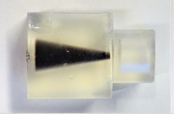
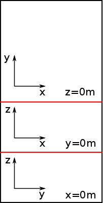
Figure 1: “Shape” phantom from the open MPI dataset (left) and visualization structure for the 3D reconstructions (right).

4.1 The benefit of whitening

First, we illustrate the benefit of whitening in the standard reconstruction technique (i.e., STD). Due to the small number of repetitions of the empty measurements (1000 repetitions compared to 23482 indices in the band limits for each receive coil, when assuming the receive coils are independent), the covariance $C$ is approximated by a diagonal one to ensure a reliable estimation. The estimated (diagonal) covariance $C$ is shown in Fig. 2. The magnitude of the noise variance is observed to vary dramatically with the frequency over the frequency band for both real and imaginary parts, and the behavior is similar for all three receive coils. The heteroscedastic nature of the noise necessitates the use of the whitening / weighting in the reconstruction algorithm as discussed in Section 2.3 in order to properly account for the noise statistics.

$x$-coil

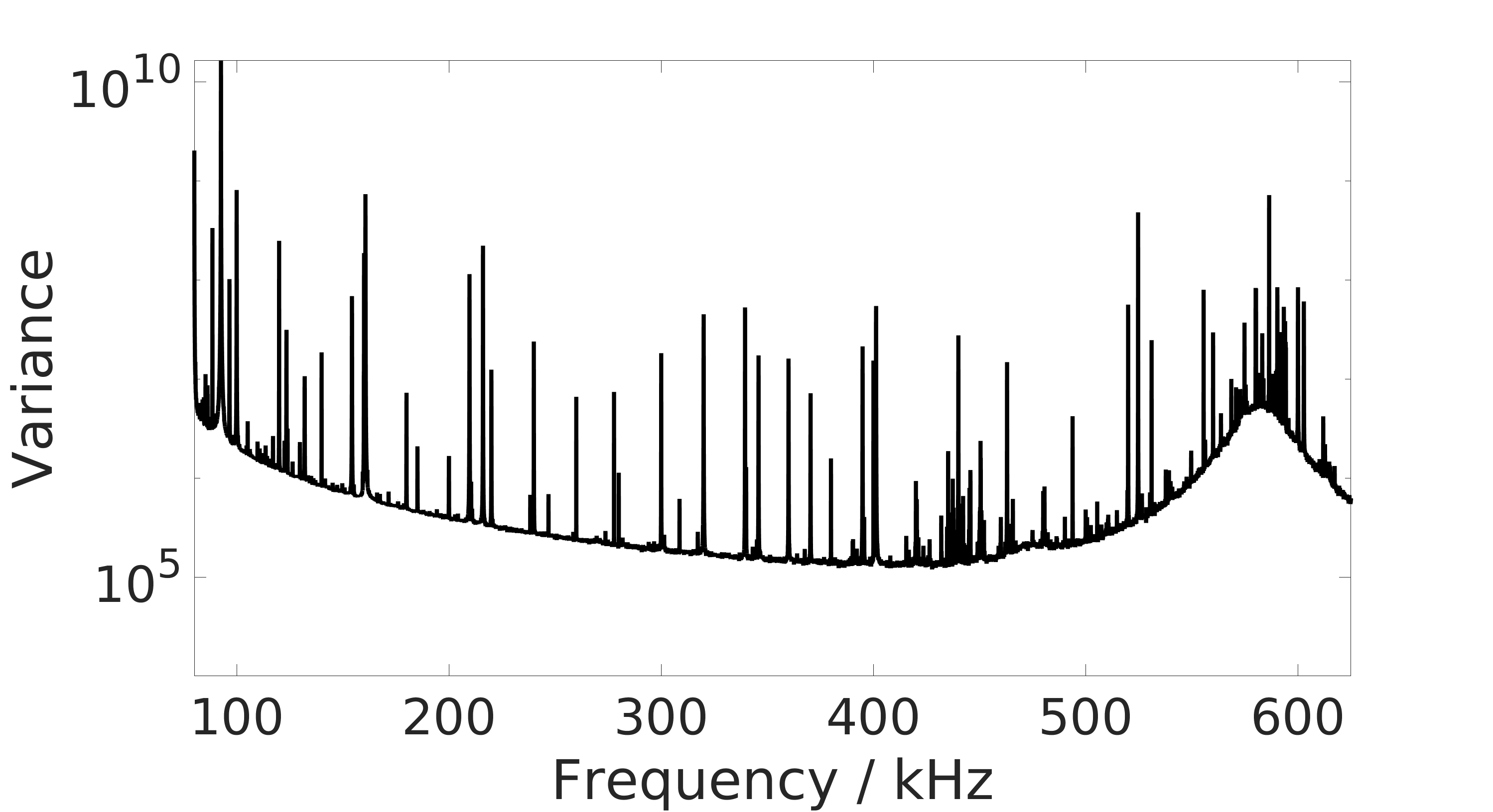
$y$-coil

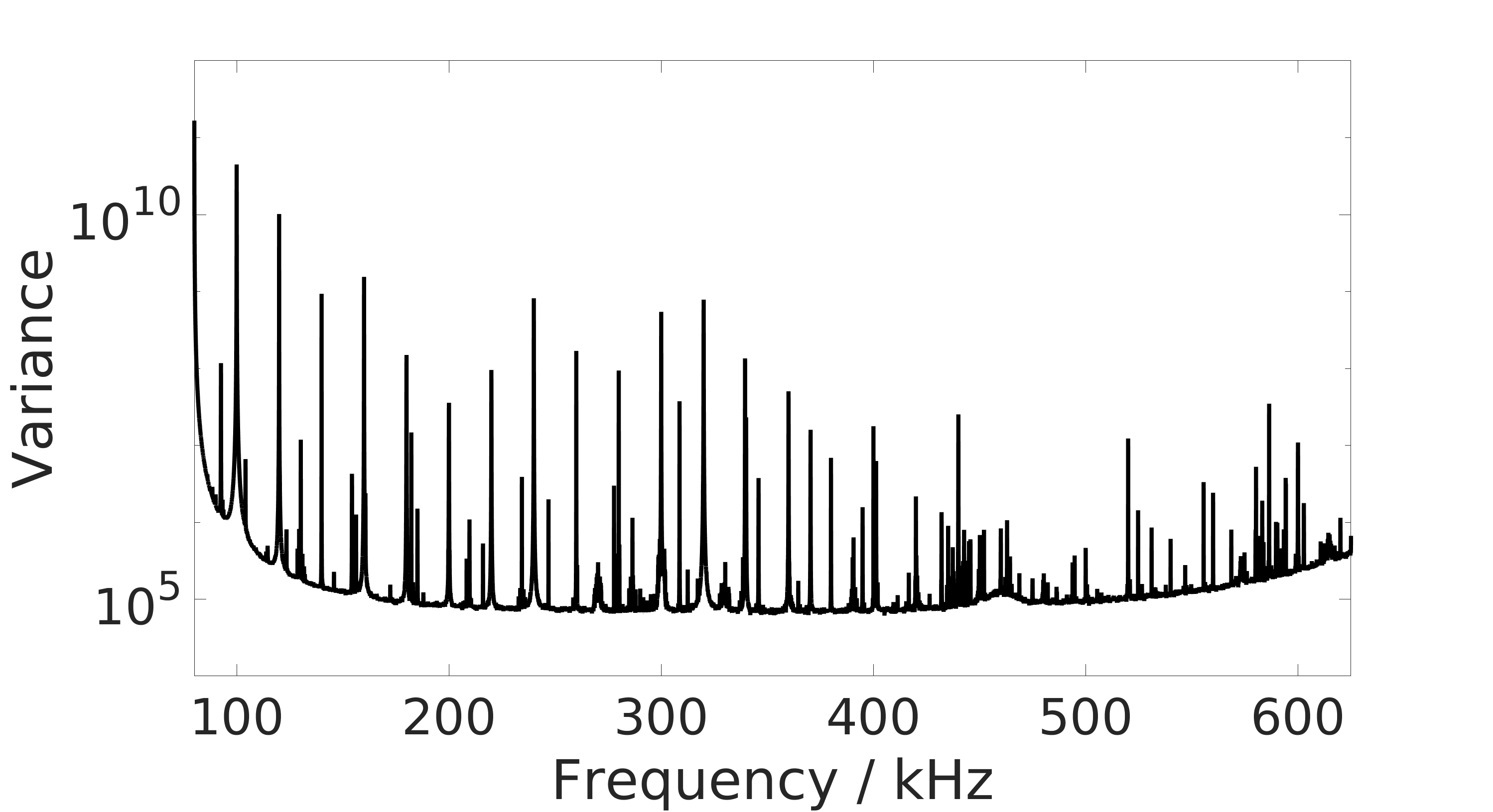
$z$-coil

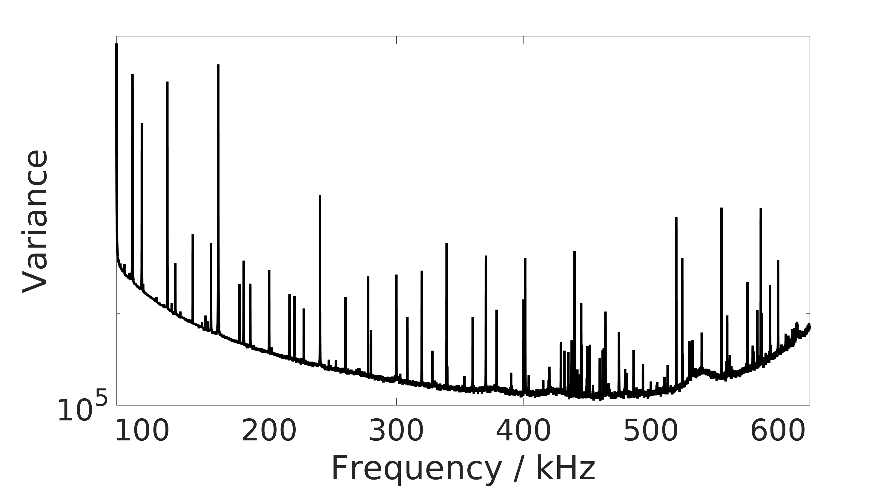
Figure 2: Variance structure of the diagonal covariance matrix $C$. Visualized individually for each receive coil with respect to the frequency; real part (top), imaginary part (bottom).

The STD reconstructions for the non-whitened and whitened cases are shown in Fig. 3, for three different $\alpha$ values, including the cases of over, medium and under regularization, respectively. For the medium and small $\alpha$ values, the reconstructed phantoms for both non-whitened and whitened cases are of similar quality; see the middle and right columns of Fig. 3. However, a closer inspection shows that the reconstruction in the non-whitened case suffers from pronounced background artifacts, whereas, in the whitened case, the artifacts can be reduced even for much smaller $\alpha$ values. Meanwhile, for a large $\alpha$ value ($\alpha=9.77\times 10^{-2}$) (the left column), the background artifacts disappear from the reconstructions in the non-whitened case but also the reconstructed cone is overly smoothed, due to over-regularization introduced by the penalty; and these observations hold also for the whitened case. Thus, the whitening step makes the reconstruction algorithm more robust to the choice of the $\alpha$ value, which is highly desirable in practice, since its optimal choice is generally very challenging.

In summary, the STD reconstructions in Fig. 3 have similar quality in the whitened and non-whited cases, except some smaller background artifacts for the non-whitened approach.

Non-whitened			Whitened
$\alpha=9.77{\mkern-2.0mu\times\mkern-2.0mu}10^{-2}$	$\alpha=3.05{\mkern-2.0mu\times\mkern-2.0mu}10^{-3}$	$\alpha=9.54{\mkern-2.0mu\times\mkern-2.0mu}10^{-5}$	$\alpha=9.77{\mkern-2.0mu\times\mkern-2.0mu}10^{-2}$	$\alpha=3.05{\mkern-2.0mu\times\mkern-2.0mu}10^{-3}$	$\alpha=9.54{\mkern-2.0mu\times\mkern-2.0mu}10^{-5}$

Figure 3: STD reconstruction non-whitened/whitened of the “shape” phantom. Illustration structure as in Fig. 1(right). Concentration in mmol/l.

4.2 Acceleration via randomized SVD

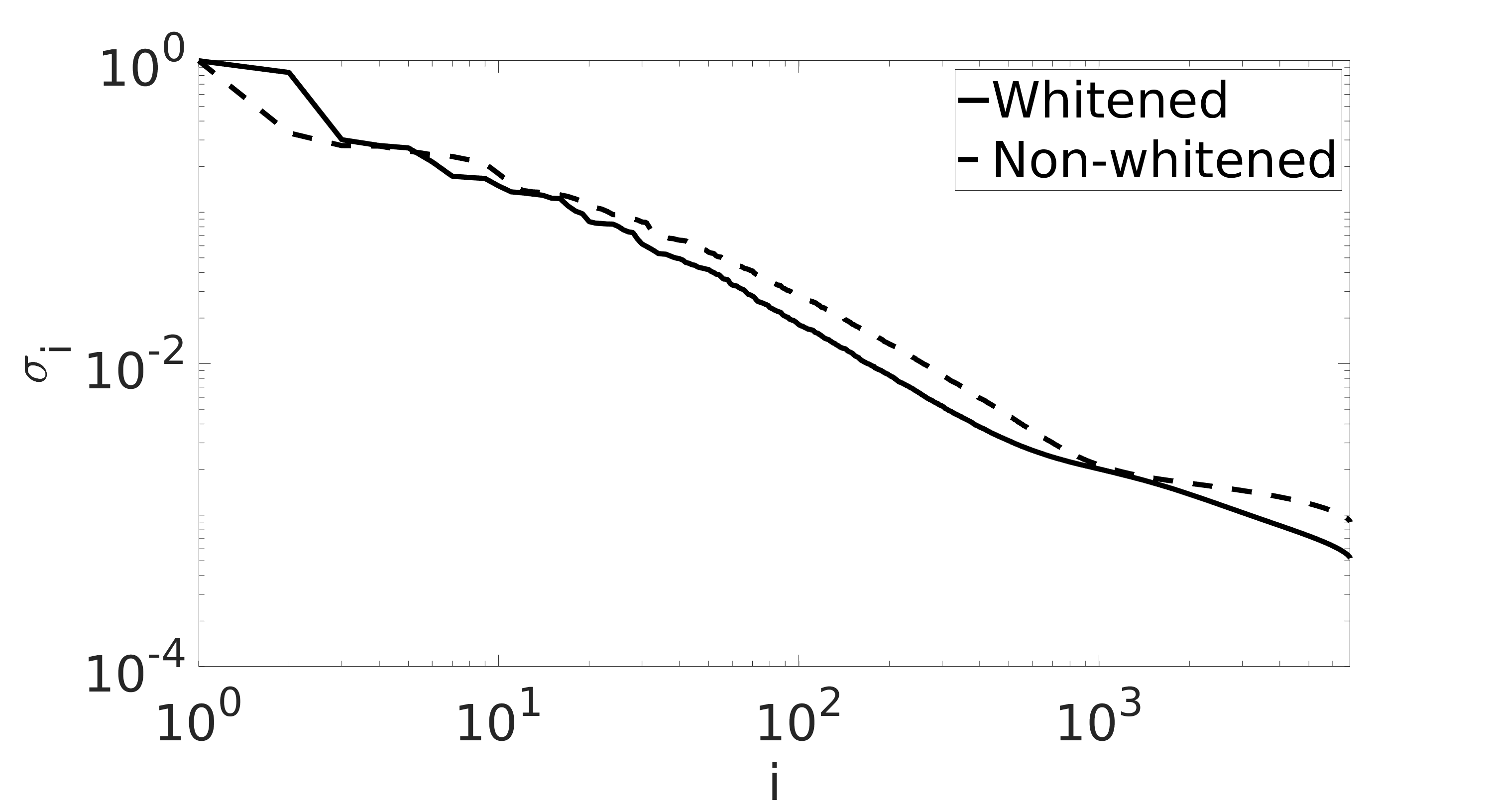
	$(\sum_{i=1}^{k}\sigma_{i}^{2})/(\sum_{i=1}^{m}\sigma_{i}^{2})$
$k$	Whitened	Non-whitened
500	99.23	99.61
1000	99.46	99.73
1500	99.55	99.80
2000	99.61	99.85

Figure 4: Illustration of singular value decay (left) of the system $A\in\mathbb{R}^{n\times m}$. Table (right) including energy percentage $(\sum_{i=1}^{k}\sigma_{i}^{2})/(\sum_{i=1}^{m}\sigma_{i}^{2})$ for low rank approximations of $A\in\mathbb{R}^{n\times m}$; relevant for constructing randomized SVD approximation.

Now we illustrate randomized SVD for accelerating the Kaczmarz algorithm, and discuss its interplay with whitening. In Fig. 4, we plot the singular values (SVs) of the non-whitened and whitened system matrices. The SVs decay algebraically with comparable decay rates for both cases, indicating that the MPI inverse problem is mildly ill-posed. A useful quantitative measure of the low-rank approximation is the percentage $(\sum_{i=1}^{k}\sigma_{i}^{2})/(\sum_{i=1}^{m}\sigma_{i}^{2})$, which roughly corresponds to the optimal error bound on the rank-$k$ approximation in the Frobenius norm. According to the table in Fig. 4, five hundred SVs capture nearly all the energies for both whitened and non-whitened cases and thus can give an accurate low rank approximation. Interestingly, in the whitened case, the same number of SVs can capture more energy percentage than that for the non-whitened case, and thus whitening may yield slightly more accurate low-rank approximations and hold more potential for speedup. The decay behavior justifies the use of the rSVD approach for accelerating the algorithm in Section 3.2. In MPI, the SV decay was rigorously proved for simplified models in [6] and [22] for the one-dimensional and multi-dimensional cases, respectively.

In view of the SV decay in Fig. 4 and the energy percentage shown in the table therein, two truncation numbers, i.e., $k=500$ and $k=1000$, are employed below for the accelerated reconstruction. The numerical results are presented in Figs. 5–7 for three different $\alpha$ values (as were used in Fig. 3), which represent over, medium and under- regularization, respectively. In these different regimes, the behavior of the reconstruction algorithms differs slightly.

With the $\alpha$ value properly chosen (i.e., $\alpha=9.77\times 10^{-2}$), rSVD1 can provide reasonable reconstructions in the whitened case for both $k$ values (cf. Fig. 6), and the reconstructions are comparable with that by STD in Fig. 3. However, in the non-whitenend case, slight blurring appears in the reconstructed cone. With the choice $k=1000$, SNR gives comparable reconstructions, but with $k=500$, either significant distortions or smoothing appear in the reconstructions for all three $\alpha$ values, and thus the choice $k=500$ seems insufficient to capture the essential information of the data. Thus, rSVD is more effective in compressing the data than SNR. Somewhat surprisingly, rSVD2, the simplest and fastest approach, can also provide reasonable reconstructions of comparable quality, even for the over-regularized case, but in the non-whitenend case, it gives reconstructions containing pronounced background artifacts, which, however, can be greatly reduced in the presence whitening; see Figs. 6 and 7. This clearly shows the significant potential of the strategy whitening + SVD2 for MPI reconstruction.

Non-whitened			Whitened
SNR	rSVD1	rSVD2	SNR	rSVD1	rSVD2
$k=1000$
$k=500$

Figure 5: “Shape” phantom reconstructions (SNR, rSVD1, rSVD2) for $\alpha=9.77{\mkern-2.0mu\times\mkern-2.0mu}10^{-2}$. Concentration in mmol/l.

Non-whitened			Whitened
SNR	rSVD1	rSVD2	SNR	rSVD1	rSVD2
$k=1000$
$k=500$

Figure 6: “Shape” phantom reconstructions (SNR, rSVD1, rSVD2) for $\alpha=3.05{\mkern-2.0mu\times\mkern-2.0mu}10^{-3}$. Concentration in mmol/l.

Non-whitened			Whitened
SNR	rSVD1	rSVD2	SNR	rSVD1	rSVD2
$k=1000$
$k=500$

Figure 7: “Shape” phantom reconstructions (SNR, rSVD1, rSVD2) for $\alpha=9.54{\mkern-2.0mu\times\mkern-2.0mu}10^{-5}$. Concentration in mmol/l.

Next we focus on the role of whitening in rSVD acceleration. Whitening influences greatly both rSVD1 and rSVD2, especially when the $\alpha$ value is small: The whitened reconstructions are of better quality since the background artifacts are strongly reduced; see Fig. 7. Note that for small $\alpha$, a small truncation number $k$ can be very beneficial for improving reconstruction quality, due to its intrinsic regularizing effect (in a manner similar to the classical truncated SVD [5]). Further, comparing $k=500$ for rSVD1 in Figs. 6 and 7, e.g., in the $x$-$y$-plane shows that whitening may enables further dimension reduction while maintaining reconstruction quality (due to the change in the SV decay curve), concurring with the observation from Fig. 4. Among the three methods under analysis, rSVD2 benefits most from whitening, since for all three $\alpha$ values, the background artifacts disappear almost completely. While the precise mechanism remains unclear, it may be attributed to the more robust SVD without too noisy singular functions corresponding to large singular values. These observations indicate that whitening is advantageous in the reconstruction: it enables using smaller $\alpha$ values in rSVD1 and rSVD2 to obtain acceptable reconstructions without unnecessary smoothing the actual phantom because of using for a sufficiently large $\alpha$, cf. Fig. 5. However, SNR benefits little from whitening: it relies on the SNR-type quality measure for dimension reduction, already exploiting the background noise characteristic to a certain degree. Thus, the dimensionality is already dramatically reduced, and the remaining rows of the reduced system have a large SNR-type quality measure and are only weakly influenced by the noise.

The computing times of the reconstruction methods are summarized in Table 1, where we have ignored the cost of preprocessing (e.g., frequency selection or rSVD) since it can be carried out offline. STD is the most expensive one among all methods under consideration. The computing time for rSVD1 and SNR are more or less comparable, when using same $k$ value, due to similar complexity (more precisely, rSVD1 has slightly longer computing times due to the additional matrix-vector multiplication to project the measurement into the space spanned by the $k$ singular functions in $\tilde{U}_{k}$ respectively $\tilde{U}_{W;k}$). rSVD2 is the fastest method due to its non-iterative nature, even if one takes into account the 20 sweeps over the corresponding reduced systems for SNR and rSVD1. Thus, all the acceleration approaches can significantly reduce the overall computational cost, with the speedup factor essentially determined by the size of the reduced system. Note that the speedup is especially important, since in practice one has to choose a proper $\alpha$ value, which inevitably requires solving a fair number of optimization problems. In particular, it holds promise as a nearly online algorithm.

$k$	SNR	rSVD1	rSVD2
$500$	0.3792$\pm$0.0227	0.3880$\pm$0.0265	0.0115$\pm$0.0011
$1000$	0.7572$\pm$0.0391	0.7775$\pm$0.0403	0.0210$\pm$0.0022
$1500$	1.1489$\pm$0.0618	1.1743$\pm$0.0609	0.0300$\pm$0.0023
$2000$	1.5465$\pm$0.0910	1.5605$\pm$0.0712	0.0395$\pm$0.0022

Table 1: Computing times (in seconds) using MATLAB (on a server with 2$\times$Intel ^® Xeon^® Broadwell-EP Series Processor E5-2687W v4, 3.00 GHz, 12-Core, and 1.5 TB DDR4 PC2666 main memory), mean and standard deviation over 100 reconstructions. The computing time for STD is 53.5308$\pm$2.6653. STD for $20n$ iterations, SNR and rSVD1 for $20k$ iterations. $n=70446$ and $m=6859$ voxels.

In summary, randomized SVD can significantly accelerate the reconstruction algorithms, within which the whitening procedure is highly beneficial, while maintaining the overall accuracy.

4.3 Performance of choice rules

Last, we illustrate the performance of the two choice rules described in Section 3.3, i.e., discrepancy principle (DP) and quasi-optimality (QO) criterion. The numerical results are given in Figs. 8-10 (with the initial value $\alpha_{0}=100$ and decreasing factor $q=0.5$). Due to the challenging nature of choosing appropriate $\tau$, $\delta$, $\sigma$ and $\epsilon$ (which may also differ for the compared methods), we used the minimum of the first 50 parameters given by the geometric sequence $\alpha_{i}$ as the upper bound $\tau\delta+\sigma\epsilon$ for DP in (3.4).

Non-whitened			Whitened
	(discr.)	(quasi.)		(discr.)	(quasi.)
	$\alpha_{i^{\ast}}=1.56{\mkern-2.0mu\times\mkern-2.0mu}10^{0}$	$\alpha_{i^{\ast}}=7.81{\mkern-2.0mu\times\mkern-2.0mu}10^{-1}$		$\alpha_{i^{\ast}}=1.56{\mkern-2.0mu\times\mkern-2.0mu}10^{0}$	$\alpha_{i^{\ast}}=2.44{\mkern-2.0mu\times\mkern-2.0mu}10^{-2}$

Figure 8: $\alpha_{i^{\ast}}$ chosen as described in Figs. 9 and 10 for the STD reconstruction. Concentration in mmol/l.

In the non-whitened case, for the given choice of parameters, DP can only give reasonable results for SNR (cf. Fig. 10). This might be related to the SNR-type quality measure: it gives a reduced system with less noise in each row such that DP can terminate at smaller $\alpha$ values. In all other non-whitened methods, there might be rows with noise contributions having a larger magnitude, which causes an early stopping of the choice rule and gives strongly regularized / smoothed reconstructions (also decreased concentration values). Whitening is also not able to improve the performance of DP. These observations are in line with the well known fact that DP tends to yield overly smoothing reconstructions, by choosing a too large regularization parameter [5]. These empirical observations indicate that the delicacy of applying DP to MPI imaging, and further research is needed to make it feasible, with one crucial issue being to obtain a reliable estimate on the noise level and bounds on the modeling errors.

The QO criterion shows excellent performance in the non-whitened case except for SNR ($k=500$) and STD. In all methods the performance is further improved when combined with whitening. Particularly for the proposed methods (rSVD1, rSVD2), it has a far superior performance than DP, and for these two methods, the best performance is reached for the whitened case. When compared with DP, STD and SNR show also improved or comparable performance, except in the SNR non-whitened case for $k=500$, which, as mentioned earlier, is insufficient to capture the essential information content in the dataset (and thus does not allow accurate reconstruction due to intrinsic information loss). For the QO criterion, whitening greatly improves the performance in all cases.

Non-whitened			Whitened
SNR	rSVD1	rSVD2	SNR	rSVD1	rSVD2
$k=1000$
$\alpha_{i^{\ast}}=2.44{\mkern-2.0mu\times\mkern-2.0mu}10^{-2}$	$\alpha_{i^{\ast}}=2.44{\mkern-2.0mu\times\mkern-2.0mu}10^{-2}$	$\alpha_{i^{\ast}}=1.56{\mkern-2.0mu\times\mkern-2.0mu}10^{0}$	$\alpha_{i^{\ast}}=4.88{\mkern-2.0mu\times\mkern-2.0mu}10^{-2}$	$\alpha_{i^{\ast}}=1.22{\mkern-2.0mu\times\mkern-2.0mu}10^{-2}$	$\alpha_{i^{\ast}}=1.56{\mkern-2.0mu\times\mkern-2.0mu}10^{0}$
$k=500$
$\alpha_{i^{\ast}}=12.5{\mkern-2.0mu\times\mkern-2.0mu}10^{0}$	$\alpha_{i^{\ast}}=2.44{\mkern-2.0mu\times\mkern-2.0mu}10^{-2}$	$\alpha_{i^{\ast}}=1.56{\mkern-2.0mu\times\mkern-2.0mu}10^{0}$	$\alpha_{i^{\ast}}=9.77{\mkern-2.0mu\times\mkern-2.0mu}10^{-2}$	$\alpha_{i^{\ast}}=1.22{\mkern-2.0mu\times\mkern-2.0mu}10^{-2}$	$\alpha_{i^{\ast}}=7.27{\mkern-2.0mu\times\mkern-2.0mu}10^{-10}$

Figure 9: $\alpha_{i^{\ast}}$ chosen according to the quasi-optimality principle in (3.5). Concentration in mmol/l.

Non-whitened			Whitened
SNR	rSVD1	rSVD2	SNR	rSVD1	rSVD2
$k=1000$
$\alpha_{i^{\ast}}=2.44{\mkern-2.0mu\times\mkern-2.0mu}10^{-2}$	$\alpha_{i^{\ast}}=1.56{\mkern-2.0mu\times\mkern-2.0mu}10^{0}$	$\alpha_{i^{\ast}}=25.0{\mkern-2.0mu\times\mkern-2.0mu}10^{0}$	$\alpha_{i^{\ast}}=4.88{\mkern-2.0mu\times\mkern-2.0mu}10^{-2}$	$\alpha_{i^{\ast}}=1.56{\mkern-2.0mu\times\mkern-2.0mu}10^{0}$	$\alpha_{i^{\ast}}=25.0{\mkern-2.0mu\times\mkern-2.0mu}10^{0}$
$k=500$
$\alpha_{i^{\ast}}=4.88{\mkern-2.0mu\times\mkern-2.0mu}10^{-2}$	$\alpha_{i^{\ast}}=1.56{\mkern-2.0mu\times\mkern-2.0mu}10^{0}$	$\alpha_{i^{\ast}}=25.0{\mkern-2.0mu\times\mkern-2.0mu}10^{0}$	$\alpha_{i^{\ast}}=9.77{\mkern-2.0mu\times\mkern-2.0mu}10^{-2}$	$\alpha_{i^{\ast}}=1.56{\mkern-2.0mu\times\mkern-2.0mu}10^{0}$	$\alpha_{i^{\ast}}=25.0{\mkern-2.0mu\times\mkern-2.0mu}10^{0}$

Figure 10: $\alpha_{i^{\ast}}$ being the regularization parameter with minimal residual which is in line with the discrepancy principle in (3.4) for an appropriate choice of $\tau\delta+\sigma\epsilon$. Concentration in mmol/l.

5 Concluding remarks

In this work we have discussed several numerical issues in the MPI reconstruction from the perspective of modern inverse theory. First, we propose to include a whitening strategy and to solve a generalized least squares problem that is adapted to the noise statistics. This step can significantly improve the robustness of the algorithm and its accuracy. Second, we propose a dimension reduction strategy in the data space via randomized SVD. The randomized SVD is computationally efficient and scales to very large matrices. This step can greatly reduce the number of equations, and arrive at an accurate reduced system. The numerical results show that by combining whitening and low-rank approximation, one can obtain reconstructions of similar quality compared to the benchmark approach, but at a much lower computational complexity, and meanwhile can improve the image quality when compared with alternative system reduction approaches like SNR. Third, we described two parameter choice rules, i.e., discrepancy principle and quasi-optimality criterion, and numerically studied their performance. It is found that that the choice rules can benefit from whitening, and the quasi-optimality criterion allows a robust parameter choice with good reconstruction quality. These experimental findings indicate that the algorithmic techniques can facilitate developing fast robust MPI reconstruction algorithms.

This study has implications on several issues in the context of MPI reconstruction. The low-rank approximation provides an alternative (and complementary) to the sparse approximation approaches for the forward map [30, 29, 40]. In contrast to these works, the dimension reduction based on randomized SVD does not rely on an a priori choice of a basis for system representation, and it is optimal with respect to the (weighted) Frobenius / spectral norm. In theory, the ill-posed nature of the MPI inverse problem [22] allows a memory-efficient representation (i.e., low-rank approximation with a small $k$) without significant loss of reconstruction quality, which is also fully confirmed by the numerical results in Section 4. The proposed method also does not require an SNR-type quality measure, which is computed from the noisy measured system matrix data and empty scanner measurements [8]. The latter is utilized in the proposed method (with a sufficiently large number of repetitions) to obtain a reasonable approximation of the covariance matrix $C$ for the whitening step. In contrast to the SNR-type quality measure, the noise characteristic is incorporated via the proposed whitening strategy. The simple nature of the used background measurement correction does not require additional empty scanner measurements during the calibration, which can potentially prolong the calibration due to expensive additional robot movements [45, 43]. Finally, the optimal dimension reduction builds the basis for developing efficient online reconstructions. In this context the proposed method is advantageous since it allows more robust and faster (due to possibly much more effective dimension reduction) image reconstruction when compared with the online reconstruction approach based on the SNR-type quality measure proposed in [26].

Appendix A Error estimate

Now we give an error estimate on the approximation $\tilde{x}_{\alpha}^{\delta}$ in a general setting. Let $X$ be a Banach space, and $Y$ be a Hilbert space, and $A:X\rightarrow Y$ be a compact linear operator. Consider the following inverse problem $Ax=y^{\dagger},$ where $x\in X$. Instead of the exact data $y^{\dagger}=Ax^{\dagger}$, corresponding to the exact solution $x^{\dagger}$, we have $y^{\delta}\in Y$ with an accuracy $\delta=\|y^{\delta}-y^{\dagger}\|$. Let $\tilde{A}:X\to Y$ be an approximate forward map with $\epsilon=\|\tilde{A}-A\|$. Then we aim at finding an approximate solution $\tilde{x}_{\alpha}^{\delta}$ by means of variational regularization [16]

$$\tilde{J}_{\alpha}(x)=\tfrac{1}{2}\|\tilde{A}x-y^{\delta}\|^{2}+\alpha\psi(x),$$

where the functional $\psi:X\to\mathbb{R}_{+}\cap\{0\}$ is a convex, proper and lower-semicontinuous functional. The common choice includes $\psi(x)=\frac{1}{2}\|x\|^{2}$, $\psi(x)=\|x\|_{\ell^{1}}$ and $\psi(x)=|x|_{\rm TV}$ etc. We denote by $x_{\alpha}^{\delta}$ a minimizer to $J_{\alpha}$ and by $\tilde{x}_{\alpha}^{\delta}$ a corresponding minimizer to $\tilde{J}_{\alpha}$ with a noisy operator $\tilde{A}$. By $x^{\dagger}$, we denote a minimum-$\psi$ solution of the equation $Ax=y^{\dagger}$: $x^{\dagger}=\arg\min_{x\in X:Ax=y^{\dagger}}\psi(x)$. It is easy to see that the derivation below remains valid for in the presence of nonnegativity constraint, so long as the minimum-$\psi$ solution is feasible.

Let $\partial\psi(x)$ be the subdifferential of $\psi$ at $x$ [4]. For any $\xi\in\partial\psi(x)$, we define the Bregman distance from $x$ to $x^{\prime}$ with respect to $\xi$ by

$$d_{\xi}(x^{\prime},x)=\psi(x^{\prime})-\psi(x)-\langle\xi,x^{\prime}-x\rangle.$$

Then we have the following error estimate on the approximation $\tilde{x}_{\alpha}^{\delta}$. It may serve as a guideline for determining the accuracy of the constructed approximation $\tilde{A}$: the model error $\epsilon=\|A-\tilde{A}\|$ should be comparable with data error $\delta$ in order not to compromise the reconstruction accuracy. The proof is standard [41, 16] and it is given only for completeness.

Theorem A.1.

Assume that the exact solution $x^{\dagger}$ fulfills the following source condition: there exists $w\in Y$ such that $A^{*}w\in\partial\psi(x^{\dagger})$. Then for the minimizer $\tilde{x}_{\alpha}^{\delta}$ to the functional $\tilde{J}_{\alpha}$, there holds

$$d_{\xi}(\tilde{x}_{\alpha}^{\delta},x^{\dagger})\leq\alpha^{-1}(\epsilon\|x^{\dagger}\|+\delta)^{2}+\alpha\|w\|^{2}+\epsilon\|w\|\|x^{\dagger}-\tilde{x}_{\alpha}^{\delta}\|.$$

Proof.

By the minimizing property of $\tilde{x}_{\alpha}^{\delta}$, we obtain

$$\tfrac{1}{2}\|\tilde{A}\tilde{x}_{\alpha}^{\delta}-y^{\delta}\|^{2}+\alpha d_{\xi}(\tilde{x}_{\alpha}^{\delta},x^{\dagger})\leq\tfrac{1}{2}\|\tilde{A}x^{\dagger}-y^{\delta}\|^{2}-\alpha\langle\xi,\tilde{x}_{\alpha}^{\delta}-x^{\dagger}\rangle.$$

Under the source condition, rearranging the inequality yields

$$\tfrac{1}{2}\|\tilde{A}\tilde{x}_{\alpha}^{\delta}-y^{\delta}\|^{2}+\alpha d_{\xi}(\tilde{x}_{\alpha}^{\delta},x^{\dagger}) \leq\tfrac{1}{2}\|\tilde{A}x^{\dagger}-y^{\delta}\|^{2}-\alpha\langle w,A(\tilde{x}_{\alpha}^{\delta}-x^{\dagger})\rangle.$$

Next we rewrite the terms on the right hand side as

$$\|\tilde{A}x^{\dagger}-y^{\delta}\|^{2} =\|\tilde{A}\tilde{x}_{\alpha}^{\delta}-y^{\delta}\|^{2}+2\langle\tilde{A}\tilde{x}_{\alpha}^{\delta}-y^{\delta},\tilde{A}(x^{\dagger}-\tilde{x}_{\alpha}^{\delta})\rangle+\|\tilde{A}(x^{\dagger}-\tilde{x}_{\alpha}^{\delta})\|^{2},$$

$$\langle w,A(\tilde{x}_{\alpha}^{\delta}-x^{\dagger})\rangle =\langle w,A_{k}(\tilde{x}_{\alpha}^{\delta}-x^{\dagger})\rangle+\langle w,(A-A_{k})(\tilde{x}_{\alpha}^{\delta}-x^{\dagger})\rangle.$$

Combining the last three estimates yields

$$\tfrac{1}{2}\|\tilde{A}\tilde{x}_{\alpha}^{\delta}-y^{\delta}\|^{2}+\alpha d_{\xi}(\tilde{x}_{\alpha}^{\delta},x^{\dagger})\leq \tfrac{1}{2}\|\tilde{A}\tilde{x}_{\alpha}^{\delta}-y^{\delta}\|^{2}+\langle\tilde{A}\tilde{x}_{\alpha}^{\delta}-y^{\delta},\tilde{A}(x^{\dagger}-\tilde{x}_{\alpha}^{\delta})\rangle+\tfrac{1}{2}\|\tilde{A}(x^{\dagger}-\tilde{x}_{\alpha}^{\delta})\|^{2}$$

$$+\alpha\langle w,\tilde{A}(x^{\dagger}-\tilde{x}_{\alpha}^{\delta})\rangle+\alpha\langle w,(A-\tilde{A})(x^{\dagger}-\tilde{x}_{\alpha}^{\delta})\rangle$$

$$= \tfrac{1}{2}\|\tilde{A}\tilde{x}_{\alpha}^{\delta}-y^{\delta}\|^{2}+\langle\tilde{A}x^{\dagger}-y^{\delta},\tilde{A}(x^{\dagger}-\tilde{x}_{\alpha}^{\delta})\rangle-\tfrac{1}{2}\|\tilde{A}(x^{\dagger}-\tilde{x}_{\alpha}^{\delta})\|^{2}$$

$$+\alpha\langle w,\tilde{A}(x^{\dagger}-\tilde{x}_{\alpha}^{\delta})\rangle+\alpha\langle w,(A-\tilde{A})(x^{\dagger}-\tilde{x}_{\alpha}^{\delta})\rangle.$$

Collecting the terms, we obtain

$$\tfrac{1}{2}\|\tilde{A}(x^{\dagger}-\tilde{x}_{\alpha}^{\delta})\|^{2}+\alpha d_{\xi}(\tilde{x}_{\alpha}^{\delta},x^{\dagger})\leq\langle\tilde{A}x^{\dagger}-y^{\delta},\tilde{A}(x^{\dagger}-\tilde{x}_{\alpha}^{\delta})\rangle+\alpha\langle w,\tilde{A}(x^{\dagger}-\tilde{x}_{\alpha}^{\delta})\rangle+\alpha\langle w,(A-\tilde{A})(x^{\dagger}-\tilde{x}_{\alpha}^{\delta})\rangle$$

Thus, by means of Cauchy-Schwarz inequality and Young’s inequality,

$$\alpha d_{\xi}(\tilde{x}_{\alpha}^{\delta},x^{\dagger})\leq\|\tilde{A}x^{\dagger}-y^{\delta}\|^{2}+\alpha^{2}\|w\|^{2}+\alpha\|w\|\|A-\tilde{A}\|\|x^{\dagger}-\tilde{x}_{\alpha}^{\delta}\|.$$

Meanwhile by the triangle inequality,

$$\|\tilde{A}x^{\dagger}-y^{\delta}\| \leq\|(\tilde{A}-A)x^{\dagger}\|+\|Ax^{\dagger}-y^{\delta}\|$$

$$\leq\|\tilde{A}-A\|\|x^{\dagger}\|+\|y^{\dagger}-y^{\delta}\|\leq\epsilon\|x^{\dagger}\|+\delta.$$

Upon substituting the estimate, we obtain

$$d_{\xi}(\tilde{x}_{\alpha}^{\delta},x^{\dagger})\leq\alpha^{-1}(\epsilon\|x^{\dagger}\|+\delta)^{2}+\alpha\|w\|^{2}+\epsilon\|w\|\|x^{\dagger}-\tilde{x}_{\alpha}^{\delta}\|.$$

This completes the proof of the theorem. ∎

Remark A.1.

For the quadratic penalty $\psi(x)=\frac{1}{2}\|x\|^{2}$, the associated Bregman distance $d_{\xi}(x^{\prime},x)$ is given by $d_{\xi}(x^{\prime},x)=\frac{1}{2}\|x^{\prime}-x\|^{2}$, and thus the error estimate in Theorem A.1 reduces to

$$\|\tilde{x}_{\alpha}^{\delta}-x^{\dagger}\|^{2}\leq 2\alpha^{-1}(\epsilon\|x^{\dagger}\|+\delta)^{2}+2\alpha\|w\|^{2}+2\epsilon\|w\|\|x^{\dagger}-\tilde{x}_{\alpha}^{\delta}\|,$$

which together with Young’s inequality yields

$$\|\tilde{x}_{\alpha}^{\delta}-x^{\dagger}\|^{2}\leq 4\alpha^{-1}(\epsilon\|x^{\dagger}\|+\delta)^{2}+4\alpha\|w\|^{2}+4\epsilon^{2}\|w\|^{2}.$$

The estimate shows that roughly one should choose $\epsilon:=\|A-\tilde{A}\|$ such that $\epsilon\|x^{\dagger}\|\approx\delta$, in order to ensure that the overall accuracy is not compromised. This directly gives a guiding principle for constructing the low-rank approximation $\tilde{A}$ in Section 3.2. Note that the last term in the estimate is generally of high order, and the first two terms essentially determines the accuracy.

References

- [1] C. Brandt and A. Seppänen. Recovery from errors due to domain truncation in magnetic particle imaging: Approximation error modeling approach. J. Math. Imag. Vis., 60(8):1196–1208, 2018.
- [2] A. Dax. On row relaxation methods for large constrained least squares problems. SIAM J. Sci. Comput., 14(3):570–584, 1993.
- [3] S. Dittmer, T. Kluth, P. Maass, and D. O. Baguer. Regularization by architecture: A deep prior approach for inverse problems. Preprint, arXiv:1812.03889, 2018.
- [4] I. Ekeland and R. Témam. Convex Analysis and Variational Problems. SIAM, Philadelphia, PA, 1999.
- [5] H. W. Engl, M. Hanke, and A. Neubauer. Regularization of Inverse Problems. Kluwer, Dordrecht, 1996.
- [6] W. Erb, A. Weinmann, M. Ahlborg, C. Brandt, G. Bringout, T. M. Buzug, J. Frikel, C. Kaethner, T. Knopp, T. März, M. Möddel, M. Storath, and A. Weber. Mathematical analysis of the 1D model and reconstruction schemes for magnetic particle imaging. Inverse Problems, 34(5):055012, 21 pp., 2018.
- [7] J. Franke, U. Heinen, H. Lehr, A. Weber, F. Jaspard, W. Ruhm, M. Heidenreich, and V. Schulz. System characterization of a highly integrated preclinical hybrid MPI-MRI scanner. IEEE Trans. Med. Imag., 35(9):1993–2004, 2016.
- [8] J. Franke, R. Lacroix, H. Lehr, M. Heidenreich, U. Heinen, and V. Schulz. MPI flow analysis toolbox exploiting pulsed tracer information - an aneurysm phantom proof. Int. J. Magnetic Particle Imag., 3(1):Article ID 1703020, 5 pp., 2017.
- [9] J. Friedman, T. Hastie, and R. Tibshirani. Sparse inverse covariance estimation with the graphical lasso. Biostatistics, 9(3):432–441, 2008.
- [10] B. Gleich and J. Weizenecker. Tomographic imaging using the nonlinear response of magnetic particles. Nature, 435(7046):1214–1217, 2005.
- [11] G. H. Golub and C. F. Van Loan. Matrix Computations. Johns Hopkins University Press, Baltimore, MD, third edition, 1996.
- [12] J. Haegele, J. Rahmer, B. Gleich, J. Borgert, H. Wojtczyk, N. Panagiotopoulos, T. Buzug, J. Barkhausen, and F. Vogt. Magnetic particle imaging: visualization of instruments for cardiovascular intervention. Radiology, 265(3):933–938, 2012.
- [13] N. Halko, P. G. Martinsson, and J. A. Tropp. Finding structure with randomness: probabilistic algorithms for constructing approximate matrix decompositions. SIAM Rev., 53(2):217–288, 2011.
- [14] U. Hämarik, U. Kangro, S. Kindermann, and K. Raik. Semi-heuristic parameter choice rules for tikhonov regularisation with operator perturbations. J. Inv. Ill-Posed Probl., pages in press. https://doi.org/10.1515/jiip–2018–0062, 2018.
- [15] G. T. Herman, A. Lent, and P. H. Lutz. Relaxation method for image reconstruction. Comm. ACM, 21(2):152–158, 1978.
- [16] K. Ito and B. Jin. Inverse Problems: Tikhonov Theory and Algorithms. World Scientific Publishing Co. Pte. Ltd., Hackensack, NJ, 2015.
- [17] Y. Jiao, B. Jin, and X. Lu. Preasymptotic convergence of randomized Kaczmarz method. Inverse Problems, 33(12):125012, 21 pp., 2017.
- [18] B. Jin and D. A. Lorenz. Heuristic parameter-choice rules for convex variational regularization based on error estimates. SIAM J. Numer. Anal., 48(3):1208–1229, 2010.
- [19] S. Kaczmarz. Angenäherte auflösung von systemen linearer gleichungen. Bull. Int. Acad. Polon. Sci. Lett. A, 35:335–357, 1937. English transl.: Int. J. Control 57(6), 1269–1271, 1993.
- [20] A. Khandhar, P. Keselman, S. Kemp, R. Ferguson, P. Goodwill, S. Conolly, and K. Krishnan. Evaluation of peg-coated iron oxide nanoparticles as blood pool tracers for preclinical magnetic particle imaging. Nanoscale, 9(3):1299–1306, 2017.
- [21] T. Kluth. Mathematical models for magnetic particle imaging. Inverse Problems, 34(8):083001, 27 pp., 2018.
- [22] T. Kluth, B. Jin, and G. Li. On the degree of ill-posedness of multi-dimensional magnetic particle imaging. Inverse Problems, 34(9):095006, 26 pp., 2018.
- [23] T. Kluth and P. Maass. Model uncertainty in magnetic particle imaging: Nonlinear problem formulation and model-based sparse reconstruction. Int. J. Magnetic Part. Imag., 3(2):1707004, 10 pp., 2017.
- [24] T. Knopp, S. Biederer, T. F. Sattel, and T. M. Buzug. Singular value analysis for magnetic particle imaging. In IEEE Nuclear Science Symposium Conference Record 2008, pages 4525–4529, 2008.
- [25] T. Knopp, N. Gdaniec, and M. Möddel. Magnetic particle imaging: from proof of principle to preclinical applications. Phys. Med. Biol., 67(14):R124–R178, 2017.
- [26] T. Knopp and M. Hofmann. Online reconstruction of 3D magnetic particle imaging data. Phys. Med. Biol., 61(11):N257–67, 2016.
- [27] T. Knopp, J. Rahmer, T. F. Sattel, S. Biederer, J. Weizenecker, B. Gleich, J. Borgert, and T. M. Buzug. Weighted iterative reconstruction for magnetic particle imaging. Phys. Med. Biol., 55(6):1577–1589, 2010.
- [28] T. Knopp, T. Viereck, G. Bringout, M. Ahlborg, A. von Gladiss, C. Kaethner, A. Neumann, P. Vogel, J. Rahmer, and M. Möddel. MDF: Magnetic particle imaging data format. Preprint, arXiv:1602.06072, 2016.
- [29] T. Knopp and A. Weber. Local system matrix compression for efficient reconstruction in magnetic particle imaging. Adv. Math. Phys., 2015:article ID 472818, 7 pp., 2015.
- [30] J. Lampe, C. Bassoy, J. Rahmer, J. Weizenecker, H. Voss, B. Gleich, and J. Borgert. Fast reconstruction in magnetic particle imaging. Phys. Med. Biol., 57(4):1113–1134, 2012.
- [31] N. Löwa, P. Radon, O. Kosch, and F. Wiekhorst. Concentration dependent MPI tracer performance. Int. J. Magnetic Particle Imag., 2(1):601001, 5 pp., 2016.
- [32] P. Maass and A. Rieder. Wavelet-accelerated Tikhonov-Phillips regularization with applications. In Inverse Problems in Medical Imaging and Nondestructive Testing (Oberwolfach, 1996), pages 134–158. Springer, Vienna, 1997.
- [33] T. März and A. Weinmann. Model-based reconstruction for magnetic particle imaging in 2D and 3D. Inverse Probl. Imaging, 10(4):1087–1110, 2016.
- [34] V. A. Morozov. On the solution of functional equations by the method of regularization. Soviet Math. Dokl., 7:414–417, 1966.
- [35] K. Murase, M. Aoki, N. Banura, K. Nishimoto, A. Mimura, T. Kuboyabu, and I. Yabata. Usefulness of magnetic particle imaging for predicting the therapeutic effect of magnetic hyperthermia. Open J. Med. Imag., 5(02):85, 2015.
- [36] F. Natterer. The Mathematics of Computerized Tomography. B. G. Teubner, Stuttgart; John Wiley & Sons, Ltd., Chichester, 1986.
- [37] J. Rahmer, A. Halkola, B. Gleich, I. Schmale, and J. Borgert. First experimental evidence of the feasibility of multi-color magnetic particle imaging. Phys. Med. Biol., 60(5):1775–1791, 2015.
- [38] Y. Saad. Iterative Methods for Sparse Linear Systems. SIAM, Philadelphia, PA, second edition, 2003.
- [39] J. Salamon, M. Hofmann, C. Jung, M. G. Kaul, F. Werner, K. Them, R. Reimer, P. Nielsen, A. vom Scheidt, G. Adam, T. Knopp, and H. Ittrich. Magnetic particle/magnetic resonance imaging: In-vitro mpi-guided real time catheter tracking and 4d angioplasty using a road map and blood pool tracer approach. PloS One, 11(6):e0156899–14, 2016.
- [40] L. Schmiester, M. Möddel, W. Erb, and T. Knopp. Direct image reconstruction of Lissajous type magnetic particle imaging data using Chebyshev-based matrix compression. IEEE Trans. Comput. Imag., 3(4):671–681, 2017.
- [41] T. Schuster, B. Kaltenbacher, B. Hofmann, and K. S. Kazimierski. Regularization Methods in Banach Spaces. Walter de Gruyter GmbH & Co. KG, Berlin, 2012.
- [42] M. Storath, C. Brandt, M. Hofmann, T. Knopp, J. Salamon, A. Weber, and A. Weinmann. Edge preserving and noise reducing reconstruction for magnetic particle imaging. IEEE Trans. Med. Imag., 36(1):74–85, 2017.
- [43] K. Them, M. G. Kaul, C. Jung, M. Hofmann, T. Mummert, F. Werner, and T. Knopp. Sensitivity enhancement in magnetic particle imaging by background subtraction. IEEE Trans. Med. Imag., 35(3):893–900, 2016.
- [44] A. N. Tihonov, V. B. Glasko, and J. A. Kriksin. On the question of quasi-optimal choice of a regularized approximation. Dokl. Akad. Nauk SSSR, 248(3):531–535, 1979.
- [45] J. Weizenecker, B. Gleich, J. Rahmer, H. Dahnke, and J. Borgert. Three-dimensional real-time in vivo magnetic particle imaging. Phys. Med. Biol., 54(5):L1–L10, 2009.
- [46] E. Y. Yu, M. Bishop, B. Zheng, R. M. Ferguson, A. P. Khandhar, S. J. Kemp, K. M. Krishnan, P. W. Goodwill, and S. M. Conolly. Magnetic particle imaging: A novel in vivo imaging platform for cancer detection. Nano Letters, 17(3):1648–1654, 2017.