Performance Analysis of Joint Radar and Communication using OFDM and OTFS

Abstract

We consider a joint radar estimation and communication system using orthogonal frequency division multiplexing (OFDM) and orthogonal time frequency space (OTFS) modulations. The scenario is motivated by vehicular applications where a vehicle equipped with a mono-static radar wishes to communicate data to its target receiver, while estimating parameters of interest related to this receiver. By focusing on the case of a single target, we derive the maximum likelihood (ML) estimator and the Cramér-Rao lower bound on joint velocity and range estimation. Numerical examples demonstrate that both digital modulation formats can achieve as accurate range/velocity estimation as state-of-the-art radar waveforms such as frequency modulated continuous wave (FMCW) while sending digital information at their full achievable rate. We conclude that it is possible to obtain significant data transmission rate without compromising the radar estimation capabilities of the system.

I Introduction

The key-enabler of high-mobility networks is the ability to continuously track the dynamically changing environment (state) and react accordingly by exchanging information with each other. The high cost of spectrum and hardware will inevitably encourage that both state estimation and communication shall be operated by sharing the same frequency bands. Towards emerging applications such as vehicular to everything (V2X), we consider a joint radar and communication system where a radar equipped transmitter (vehicle) wishes to estimate the parameters of a target receiver and simultaneously send data to this receiver, as already investigated in the literature (see [1, 2, 3] and references therein). Although most of existing works build on a resource-sharing approach such that time or frequency resources are split into either radar estimation or data communication [2, 3], a synergetic design can potentially yield a significant performance gain, as demonstrated in an information theoretic framework [4]. Motivated by this result, we study the performance of a joint radar and communication system using two digital modulation formats, namely, the well-known orthogonal frequency division multiplexing (OFDM) and the recently proposed orthogonal time frequency space (OTFS) (see [5] and references therein).

By focusing on a single-target case, we characterize the joint radar and communication performance in terms of mean square error (MSE) and achievable rate. More precisely, the maximum likelihood (ML) estimator and the Cramér-Rao lower bound (CRLB) on velocity and range estimation are derived. Our numerical examples, inspired by the parameters of IEEE 802.11p, demonstrate that both waveforms provide similar radar performance while OTFS yields better multiplexing gain than OFDM. Surprisingly, the two waveforms perform similarly as frequency modulated continuous wave (FMCW), one of the typical automotive radar waveforms [6], while achieving a significant communication rate for free.

It is worth noticing that OFDM has been extensively studied for radar estimation (see [1, 7, 3] and references therein). However, none of these works has addressed explicitly the joint performance in terms of MSE and achievable communication rate. A comparison of radar estimation between OTFS and OFDM has been independently developed in a very recent work [8]. By neglecting part of the fractional Doppler and delay shifts and further focusing on a low-complexity matched filter approach for OTFS, this work concluded that OTFS has some advantages over OFDM since it can handle larger Doppler shifts and longer range. In contrast, the current work considers ML estimator without neglecting the fractional part of Doppler and delay shifts, while restricting to Doppler shifts of practical relevance for automotive applications, such that the inter-carrier interference (ICI) incurred by OFDM is definitely negligible. Under these conditions, we obtain different conclusions as [8].

The paper is organized as follows. In section II we present the physical model. In section III and IV, we derive the ML estimator and the CRLB for OFDM and OTFS, respectively. Section V provides numerical results and Section VI concludes the paper.

II Physical model

We consider a joint radar and communication system over a total bandwidth of $B$ [Hz] operating at the carrier frequency $f_{c}$ [Hz]. We assume that a transmit vehicle, equipped with a mono-static full-duplex radar, wishes to convey a message to its target receiver while estimating parameters related to the same receiver. For simplicity, we focus on a point target model, so that the link between a transmitter and a receiver can be represented by as a single line-of-sight channel [9, 2]. In a multi-carrier system, the total bandwidth is divided into $M$ subcarriers, i.e., $B=M\Delta f$, where $\Delta f$ [Hz] denotes the subcarrier bandwidth. For a given maximum delay $\tau_{\max}$ and a given maximum Doppler shift $\nu_{\max}$, the symbol duration $T$ and the subcarrier spacing $\Delta f$ are chosen to satisfy

$$\nu_{\max}<\Delta f\,,\quad\tau_{\max}<T\,,$$ (1)

with $T=1/\Delta f$. Suppose there are $P$ targets and the $p$-th target vehicle is at the relative range of $r_{p}$ [m] and is moving at the relative velocity of $v_{p}$ [m/sec] with respect to the transmitter. We model the radar channel as a $P$-tap time frequency selective channel given by

$$h(t,\tau)=\sum_{p=0}^{P-1}h_{p}\delta(\tau-\tau_{p})e^{j2\pi\nu_{p}t}\,,$$ (2)

where $h_{p}$ is the complex channel gain, $\nu_{p}=\frac{2v_{p}f_{c}}{c}$ and $\tau_{p}=\frac{2r_{p}}{c}$ denotes a round-trip Doppler shift and delay, respectively. By taking into account the one-way Doppler shift and delay, the forward communication channel is given by

$$h_{\rm com}(t,\tau)={g_{0}}e^{j\pi\nu_{0}t}\delta\left(\tau-\frac{\tau_{0}}{2}\right)\,,$$ (3)

where $g_{0}$ denotes the complex channel gain. In both OFDM and OTFS, data symbols $x_{n,m}$, for $n=0,\dots,N-1$ and $m=0,\dots,M-1$, are arranged in an $N\times M$ grid $\Lambda$, and satisfy the average power constraint, i.e.

$$\frac{1}{NM}\sum_{n=0}^{N-1}\sum_{m=0}^{M-1}\mathbb{E}\left[\left|x_{n,m}\right|^{2}\right]\leq P_{\mathrm{avg}}\,.$$ (4)

III OFDM

III-A Input Output Relation

Consider a standard OFDM modulation with cyclic prefix (CP) in order to avoid the inter-symbol interference (ISI). The resulting OFDM symbol duration is $T_{o}=T_{\rm cp}+T$, where $T_{\rm cp}$ and $T$ denote the CP and data symbols duration, respectively. Provided the maximum delay $\tau_{\max}$ we typically choose $T_{\rm cp}=C\frac{T}{M}$, with $C=\lceil\frac{\tau_{\max}}{T/M}\rceil$, where $\lceil\cdot\rceil$ is the rounding-up operation. The OFDM frame duration is thus $T_{f}^{\rm ofdm}=NT_{o}$. The continuous-time OFDM transmitted signal with CP is given by

$$s(t)=\sum_{n=0}^{N-1}\sum_{m=0}^{M-1}x_{n,m}{\rm rect}(t-nT_{o})e^{j2\pi m\Delta f(t-T_{\rm cp}-nT_{o})}\,,$$ (5)

where ${\rm rect}(t)$ is one for $t\in[0,T_{o}]$ and zero otherwise. Ignoring the noise, the signal received after the time-frequency selective channel (2) is

$$y^{\prime}(t)=\int h(t,\tau)s(t-\tau)d\tau=\sum_{p=0}^{P-1}h_{p}s(t-\tau_{p})e^{j2\pi\nu_{p}t}\,.$$ (6)

By sampling every $\frac{T}{M}$ and removing the CP in each OFDM symbol, we obtain

$$y^{\prime}_{n,m} =y^{\prime}(t)|_{t=nT_{o}+T_{\rm cp}+m{T}/{M}}=\sum_{p=0}^{P-1}h_{p}e^{j2\pi nT_{o}\nu_{p}}$$

$$\sum_{m^{\prime}=0}^{M-1}x_{n,m^{\prime}}e^{j2\pi\frac{m}{M}\left(\frac{\nu_{p}}{\Delta f}+m^{\prime}\right)}e^{-j2\pi{m^{\prime}}\Delta f\tau_{p}}\,.$$ (7)

Applying the discrete Fourier transform (DFT) and using the orthogonal property, the output is given by

$$y_{n,m} =\frac{1}{M}\sum_{i=0}^{M-1}y^{\prime}_{n,i}e^{-j2\pi\frac{mi}{M}}$$

$$\approx\sum_{p=0}^{P-1}h_{p}e^{j2\pi nT_{o}\nu_{p}}e^{-j2\pi{m}\Delta f\tau_{p}}x_{n,m}\,,$$ (8)

where the approximation follows by letting $\nu_{\max}\ll\Delta f$. Under the approximated channel input-output relation (III-A), it readily follows that the Doppler shift and the delay are decoupled, which makes joint range and velocity estimation simple (see e.g. [7, 1]). By focusing for simplicity on a single-target case ($P=1$), we neglect the $p$-path subscript from now on. Since data symbols are known by the radar receiver (the transmitter itself), and the noise is i.i.d. Gaussian circularly symmetric, the radar receiver can undo the data symbol phase without changing the noise statistics. Therefore, the radar observation after this symbol-by-symbol phase rotations can be written as

$$z_{n,m}=A_{n,m}he^{j2\pi nT_{o}\nu}e^{-j2\pi m\Delta f\tau}+w_{n,m}\,,$$ (9)

where $A_{n,m}=\left|x_{n,m}\right|$ denotes the amplitude of the transmitted symbol and $w_{n,m}$ is additive white Gaussian noise (AWGN) with zero mean and unit variance.

III-B Maximum Likelihood Estimator

We derive the ML estimator of channel gain/range/velocity for the observation model in (9) by generalizing [7, Chapter 3.3.3] to the case of arbitrarily amplitude $\boldsymbol{A}$, with $\boldsymbol{A}=\{A_{n,m}\}$. For the set of parameters $\boldsymbol{\theta}=(h,\nu,\tau)$, we wish to find the estimator minimizing the log-likelihood function

$$l(\boldsymbol{z}|\boldsymbol{\theta},\boldsymbol{A})=\sum_{n}\sum_{m}\left|z_{n,m}-hA_{n,m}e^{j2\pi\left(\nu nT_{o}-m\Delta f\tau\right)}\right|^{2}.$$ (10)

Assuming $(\nu,\tau)$ known, by setting the derivative of $l(\boldsymbol{z}|\boldsymbol{\theta},\boldsymbol{A})$ with respect to $h$ equal to zero, we obtain the estimator $\hat{h}$ of the complex channel gain $h$, which is

$$\hat{h}=\frac{Z(\nu,\tau)}{\sum_{n,m}A^{2}_{n,m}}\,,$$ (11)

where we defined a DFT/ inverse discrete Fourier transform (IDFT) operation as

$$Z(\nu,\tau)\triangleq\sum_{m=0}^{M-1}\sum_{n=0}^{N-1}z_{n,m}A_{n,m}e^{-j2\pi\nu nT_{o}}e^{j2\pi{m}\Delta f\tau},$$ (12)

which is a two-dimensional periodogram. By plugging (11) into (10) and following similar steps as [11, Chapter 7.2.2]), we obtain the estimator

$$(\hat{\nu},\hat{\tau})=\arg\max_{(\nu,\tau)\in\Gamma}\left|Z(\nu,\tau)\right|^{2}\,,$$ (13)

where we considered a discretized set $\Gamma$ of delay and Doppler frequency axes with step sizes ${1}/\left({M^{\prime}\Delta f}\right)$ and ${1}/\left({N^{\prime}T_{\rm o}}\right)$, respectively, with $N^{\prime}\geq N$ and $M^{\prime}\geq M$.

In summary, to compute the ML estimator of $(h,\tau,\nu)$ the following steps are done:

1. Compute the DFT/IDFT output $Z(\nu,\tau)$.

2. Choose $(\hat{\nu},\hat{\tau})$ maximizing $\left|Z(\nu,\tau)\right|^{2}$ over $\Gamma$.

3. Let the channel gain be $\hat{h}={Z(\hat{\nu},\hat{\tau})}/\left(\sum_{n,m}A_{n,m}^{2}\right)$.

The resulting velocity and range radar estimations are given by $\hat{v}=\frac{\hat{\nu}c}{2f_{c}}$ and $\hat{r}=\frac{\hat{\tau}c}{2}$.

III-C CRLB

Consider the vector of unknown $\hbox{\boldmath$\theta$}=(\alpha,\varphi,f,\mathsf{t})$, where $\alpha=|h|$, $\varphi=\angle(h)$, $f=T_{o}\nu$, and $\mathsf{t}=\Delta f\tau$, from (9) we obtain

$$z_{n,m}=A_{n,m}\alpha e^{j\varphi}e^{j2\pi nf}e^{-j2\pi{m}\mathsf{t}}+w_{n,m}\,.$$ (14)

By letting $s_{n,m}=A_{n,m}\alpha e^{j\varphi}e^{j2\pi nf}e^{-j2\pi{m}\mathsf{t}}$, we derive the $4\times 4$ Fisher information matrix defined as

$$[{\bf I}(\hbox{\boldmath$\theta$},\boldsymbol{A})]_{i,j} =2P_{\mathrm{avg}}\Re\left\{\sum_{n,m}\left[\frac{\partial s_{n,m}}{\partial\theta_{i}}\right]^{*}\left[\frac{\partial s_{n,m}}{\partial\theta_{j}}\right]\right\}.$$ (15)

After straightforward algebra, we are able to prove the following result.

Lemma 1.

In the regime of large $M$ and $N$, the CRLB of $f$ and $\mathsf{t}$ are given by

$$\sigma_{\rm\hat{f}}^{2} \geq\frac{6}{|h|^{2}P_{\mathrm{avg}}(2\pi)^{2}MN({N}^{2}-1)}\,,$$ (16a)

$$\sigma_{\rm\hat{\mathsf{t}}}^{2} \geq\frac{6}{|h|^{2}P_{\mathrm{avg}}(2\pi)^{2}MN({M}^{2}-1)}\,.$$ (16b)

For a special case of constant envelope ($A_{n,m}=\sqrt{P_{\mathrm{avg}}}$ for all $n,m$), the above expressions coincide with those in [7, Section 3.3].

IV OTFS

IV-A Input Output Relation

The transmitter first applies the inverse symplectic finite Fourier transform (ISFFT) to represent data symbols $\{x_{k,l}\}$ in the time-frequency domain, i.e., $X\left[n,m\right]$, then generates the continuous time signal

$$s\left(t\right)=\sum_{n=0}^{N-1}\sum_{m=0}^{M-1}X\left[n,m\right]g_{\mathrm{tx}}\left(t-nT\right)e^{j2\pi m\Delta f\left(t-nT\right)},\,$$ (17)

where $g_{\mathrm{tx}}$ denotes a transmit pulse. The OTFS frame duration is thus $T_{f}^{\mathrm{otfs}}=NT$. The noiseless received signal $r\left(t\right)$, after the channel in (2), is given in (6). Defining the cross ambiguity function between two pulses as in [12]

$$C_{u,v}\left(\tau,\nu\right)\triangleq\int_{-\infty}^{\infty}u\left(t\right)v^{*}\left(t-\tau\right)e^{-j2\pi\nu t}dt\,,$$ (18)

the output of the matched filter is given by

$$Y\left(t,f\right)=C_{r,g_{\mathrm{rx}}}\left(t,f\right)=\int r\left(t^{\prime}\right)g_{\mathrm{rx}}^{*}\left(t^{\prime}-t\right)e^{-j2\pi ft^{\prime}}dt^{\prime}\,.$$ (19)

By sampling at $t=nT$ and $f=m\Delta f$, the received samples in the time-frequency domain are given by

$$Y\left[n,m\right] =Y\left(t,f\right)|_{t=nT,f=m\Delta f}$$

$$=\sum_{n^{\prime}=0}^{N-1}\sum_{m^{\prime}=0}^{M-1}X\left[n^{\prime},m^{\prime}\right]H_{n,m}\left[n^{\prime},m^{\prime}\right]\,,$$ (20)

where, by letting $h_{p}^{\prime}\triangleq h_{p}e^{j2\pi\nu_{p}\tau_{p}}$, we have

$$H_{n,m} \left[n^{\prime},m^{\prime}\right]\triangleq\sum_{p=0}^{P-1}h_{p}^{\prime}e^{j2\pi n^{\prime}T\nu_{p}}e^{-j2\pi m\Delta f\tau_{p}}$$

$$C_{g_{\mathrm{tx}},g_{\mathrm{rx}}}\left(\left(n-n^{\prime}\right)T-\tau_{p},\left(m-m^{\prime}\right)\Delta f-\nu_{p}\right).$$ (21)

Finally, we obtain the received samples in the Doppler-delay domain applying the symplectic finite Fourier transform (SFFT) to (IV-A), i.e.

$$y\left[k,l\right] =\frac{1}{NM}\sum_{n^{\prime}=0}^{N-1}\sum_{m^{\prime}=0}^{M-1}Y\left[n,m\right]e^{-j2\pi\left(\frac{nk}{N}-\frac{ml}{M}\right)}$$

$$=\sum_{k^{\prime}=0}^{N-1}\sum_{l^{\prime}=0}^{M-1}x_{k^{\prime},l^{\prime}}g_{k,k^{\prime}}\left[l,l^{\prime}\right]\,,$$ (22)

where the cross-talk channel of the Doppler-delay couple $\left[k^{\prime},l^{\prime}\right]$ seen by $\left[k,l\right]$ is given by

$$g_{k,k^{\prime}}\left[l,l^{\prime}\right]=\sum_{p=0}^{P-1}h_{p}^{\prime}\boldsymbol{\Psi}^{p}_{k,k^{\prime}}\left[l,l^{\prime}\right]\,,$$ (23)

with the channel matrix $\boldsymbol{\Psi}^{p}_{k,k^{\prime}}\left[l,l^{\prime}\right]$ defined in (24).

$$\boldsymbol{\Psi}^{p}_{k,k^{\prime}}\left[l,l^{\prime}\right]=\frac{1}{NM}\sum_{n,n^{\prime},m,m^{\prime}}e^{j2\pi n^{\prime}T\nu_{p}}e^{-j2\pi m\Delta\tau_{p}}e^{-j2\pi\left(\frac{nk}{N}-\frac{ml}{M}\right)}C_{g_{\mathrm{rx}},g_{\mathrm{tx}}}\left(\left(n-n^{\prime}\right)T-\tau_{p},\left(m-m^{\prime}\right)\Delta f+\nu_{p}\right)\,.$$ (24)

By stacking the $N\times M$ matrices of transmitted symbols and received samples to column vectors of length $NM$, we obtain the vector input-output relation as

$$\boldsymbol{y}=\sum_{p=0}^{P-1}h_{p}^{\prime}\boldsymbol{\Psi}^{p}\boldsymbol{x}+\boldsymbol{w}\,,$$ (25)

where $\boldsymbol{\Psi}^{p}$ is the $NM\times NM$ matrix obtained from (24), $\boldsymbol{w}$ denotes the AWGN with zero mean and identity covariance. Notice that our input-output relation in (25) is exact and holds for any pair of transmit/receive pulses.

Letting $g_{\mathrm{tx}}\left(t\right)$ and $g_{\mathrm{rx}}\left(t\right)$ be rectangular pulses of length $T$, it readily follows that the cross-ambiguity function is non-zero only for $n^{\prime}=n$ and for $n^{\prime}=n-1$ since the maximum channel delay $\tau_{\mathrm{max}}<T$. For further derivation, we consider also the approximated cross-ambiguity function given by

$$C_{g_{\mathrm{rx}},g_{\mathrm{tx}}}\left(\tau,\nu\right) =\int_{0}^{T}g_{\mathrm{tx}}\left(t\right)g_{\mathrm{rx}}^{*}\left(t-\tau\right)e^{-j2\pi\nu t}dt$$

$$\approx\frac{1}{M}\sum_{i=0}^{M-1-l_{\tau}}\exp\left(j2\pi\nu\frac{Ti}{M}\right)\,,$$ (26)

where $l_{\tau}=\lceil\frac{\tau}{T/M}\rceil$ is an integer in $[0,M-1]$. The cross-talk matrix $\boldsymbol{\Psi}^{p}_{k,k^{\prime}}\left[l,l^{\prime}\right]$ using the approximated cross ambiguity function and rectangular pulses is given in (27).

$$\ \begin{aligned} \boldsymbol{\Psi}^{p}_{k,k^{\prime}}\left[l,l^{\prime}\right]&\approx\frac{1}{NM}\frac{1-e^{j2\pi\left(k^{\prime}-k+\nu_{p}NT\right)}}{1-e^{j2\pi\frac{\left(k^{\prime}-k+\nu_{p}NT\right)}{N}}}\frac{1-e^{j2\pi\left(l^{\prime}-l+\tau_{p}M\Delta f\right)}}{1-e^{j2\pi\frac{\left(l^{\prime}-l+\tau_{p}M\Delta f\right)}{M}}}e^{j2\pi\nu_{p}\frac{l^{\prime}}{M\Delta f}}\begin{cases}\begin{array}[]{ll}1&l^{\prime}\in\left[0,M-1-l_{\tau_{p}}\right]\\ e^{-j2\pi\left(\frac{k^{\prime}}{N}+\nu_{p}T\right)}&l^{\prime}\in\left[M-l_{\tau_{p}},M-1\right]\\ \end{array}.\end{cases}\end{aligned}$$ (27)

 

IV-B Maximum Likelihood Estimator

By focusing on the single-target case $\left(P=1\right)$ and neglecting the $p$-path subscript, we wish to find the ML estimator for the set of unknown parameters $\boldsymbol{\theta}=\left(h^{\prime},\tau,\nu\right)$. The log-likelihood function to be minimized is given by

$$l\left(\boldsymbol{y}|\boldsymbol{\theta},\boldsymbol{x}\right)=\left|\boldsymbol{y}-h^{\prime}\boldsymbol{\Psi}\left(\tau,\nu\right)\right|\,,$$ (28)

where symbols in $\boldsymbol{x}$ are known at the radar receiver. We now follow the same steps as for OFDM. Assuming $\left(\tau,\nu\right)$ known, the estimator $\hat{h}^{\prime}$ of the channel gain $h^{\prime}$ is given by

$$\hat{h}^{\prime}=\frac{\boldsymbol{x}^{H}\boldsymbol{\Psi}^{H}\boldsymbol{y}}{\boldsymbol{x}^{H}\boldsymbol{\Psi}^{H}\boldsymbol{\Psi}\boldsymbol{x}}\,,$$ (29)

where $H$ indicates the transpose complex conjugate. We readily obtain the estimate $\hat{\tau},\hat{\nu}$ of $\tau,\nu$ using (29) as

$$\left(\hat{\tau},\hat{\nu}\right) =\arg\max_{\left(\tau,\nu\right)\in\Gamma}\frac{\left|\boldsymbol{x}^{H}\boldsymbol{\Psi}\left(\tau,\nu\right)^{H}\boldsymbol{y}\right|^{2}}{\boldsymbol{x}^{H}\boldsymbol{\Psi}\left(\tau,\nu\right)^{H}\boldsymbol{\Psi}\left(\tau,\nu\right)\boldsymbol{x}}\,,$$ (30)

where $\Gamma$ is specified in (13).

IV-C CRLB

In order to derive the CRLB, we use the approximated channel matrix given in (27). Referring to the Fisher information matrix in (15), we let

$$s[k,l]=\sum_{k^{\prime}=0}^{N-1}\sum_{l^{\prime}=0}^{M-1}h^{\prime}\boldsymbol{\Psi}_{k,k^{\prime}}\left[l,l^{\prime}\right]x\left[k^{\prime},l^{\prime}\right]\,.$$ (31)

Note that the channel matrix contains the two unknown parameter $\tau$ and $\nu$. In order to express the derivative, let us introduce the following indices

$$\begin{cases}l^{\prime}_{\mathrm{ICI}}\triangleq l^{\prime}\in\left[0,M-1-l_{\tau_{p}}\right]\\ l^{\prime}_{\mathrm{ISI}}\triangleq l^{\prime}\in\left[M-l_{\tau_{p}},M-1\right]\end{cases}.$$ (32)

The derivative w.r.t. $\tau$ is given by

$$\frac{\partial\boldsymbol{\Psi}_{k,k^{\prime}}\left[l,l^{\prime}\right]}{\partial\tau}=\sum_{n}e^{j2\pi\left(\nu NT-k+k^{\prime}\right)\frac{n}{N}}\sum_{m}e^{j2\pi\left(l-l^{\prime}-\tau M\Delta f\right)}$$

$$\left(-j2\pi m\Delta f\right)\frac{e^{j2\pi\nu\left(\frac{l^{\prime}}{M\Delta f}\right)}}{NM}\begin{cases}\begin{array}[]{ll}1&l^{\prime}_{\mathrm{ICI}}\\ e^{-j2\pi\left(\frac{k^{\prime}}{N}+\nu T\right)}&l^{\prime}_{\mathrm{ISI}}\end{array}.\end{cases}$$ (33)

The derivative w.r.t. $\nu$ is given by

$$\frac{\partial\boldsymbol{\Psi}_{k,k^{\prime}}\left[l,l^{\prime}\right]}{\partial\nu}=\frac{j2\pi}{NM}\sum_{m}e^{j2\pi\left(l-l^{\prime}-\tau M\Delta f\right)}e^{j2\pi\nu\left(\frac{l^{\prime}}{M\Delta f}\right)}$$

$$\Bigg{[}\sum_{n}e^{j2\pi\left(\nu NT-k+k^{\prime}\right)\frac{n}{N}}\begin{cases}\begin{array}[]{ll}\frac{l^{\prime}}{M\Delta f}&l^{\prime}_{\mathrm{ICI}}\\ e^{-j2\pi\left(\frac{k^{\prime}}{N}+\nu T\right)}\left(\frac{l^{\prime}}{M\Delta f}-T\right)&l^{\prime}_{\mathrm{ISI}}\\ \end{array}\end{cases}$$

$$+nT\sum_{n}e^{j2\pi\left(\nu NT-k+k^{\prime}\right)\frac{n}{N}}\begin{cases}\begin{array}[]{ll}1&l^{\prime}_{\mathrm{ICI}}\\ e^{-j2\pi\left(\frac{k^{\prime}}{N}+\nu T\right)}&l^{\prime}_{\mathrm{ISI}}\\ \end{array}\Bigg{]}.\end{cases}$$ (34)

The CRLB expressions follow by applying the Fisher information matrix in (15).

V Simulation Results

TABLE I: Simulation parameters

IEEE 802.11p [3]
$f_{c}=5.89$ GHz	$M=64$
$B=10$ MHz	$N=50$
$\Delta f=B/M=156.25$ kHz	$T_{\mathrm{cp}}=\frac{1}{4}T=1.6\,\mu$s
$T=1/\Delta f=6.4\,\mu s$	$T_{\mathrm{o}}=T_{\mathrm{cp}}+T=8\,\mu$s
$r^{\rm otfs}_{\mathrm{max}}<Tc/2\simeq 960$ m	$r^{\rm ofdm}_{\mathrm{max}}<T_{\rm cp}c/2\simeq 240$ m
$\sigma_{\mathrm{rcs}}=1$ m2	$G=100$
$r=20$ m	$v=80$ km/h

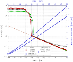
Figure 1: Root MSE (left y-axis) of the target range estimation $\hat{r}$ vs $\mathrm{SNR_{rad}}$ (bottom x-axis). The figure also shows the communication rate (right y-axis) vs $\mathrm{SNR_{com}}$ (top x-axis).

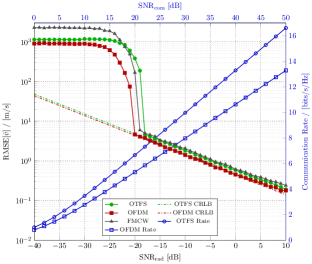
Figure 2: Root MSE (left y-axis) of the target velocity estimation $\hat{v}$ vs $\mathrm{SNR_{rad}}$ (bottom x-axis) and the communication rate as a function of $\mathrm{SNR_{com}}$ (top x-axis).

Simulation has been performed using the system model specified in Section II. Let the received radar and communication signal-to-noise ratio (SNR) be

$$\mathrm{SNR_{rad}}=\left|h_{0}\right|^{2}P_{\mathrm{avg}}\,,\quad\mathrm{SNR_{com}}=\left|g_{0}\right|^{2}P_{\mathrm{avg}}\,,$$ (35)

with

$$\left|h_{0}\right|=\sqrt{\frac{\lambda^{2}\sigma_{\mathrm{rcs}}G^{2}}{\left(4\pi\right)^{3}r^{4}}}\,,\quad\left|g_{0}\right|=\sqrt{\frac{\lambda^{2}G^{2}}{\left(4\pi\right)^{2}r^{2}}}\,,$$ (36)

where $\lambda=c/f_{c}$ is the wavelength, $\sigma_{\mathrm{rcs}}$ is the radar cross section in $\mathrm{m}^{2}$, $G$ is the antenna gain, and $r$ is the distance between transmitter and receiver. In order to characterize the joint radar and communication performance, we provide the communication rate at the communication receiver for both OFDM and OTFS

$$C_{\mathrm{OFDM}} =\left(\frac{T}{T+T_{\mathrm{cp}}}\right)\log_{2}\left(1+\mathrm{SNR_{com}}\right)\,,$$ (37a)

$$C_{\mathrm{OTFS}} =\frac{1}{NM}\log_{2}\det\left(\boldsymbol{I}+\mathrm{SNR_{com}}\boldsymbol{\Psi}\boldsymbol{\Psi}^{H}\right)\,.$$ (37b)

Using the parameters listed in Table I, we show the range estimation in terms of root MSE (RMSE) and the communication rate (37) for OFDM and OTFS in Figure 1. Similarly, Figure 2 provides the velocity estimation and the communication rate. As a reference, we show the radar performance of FMCW, as one of the popular automotive waveforms [6], using the same bandwidth and time resource. In both figures, we observe that the CRLB of the three waveforms is almost identical.

First we observe that the radar performance is similar for three waveforms. It is remarkable that OFDM and OTFS, simultaneously sending data symbols, are able to achieve as accurate performance as FMCW. Second, we remark that OTFS performs better than OFDM in terms of communication rate by achieving a higher multiplexing gain. This is because OFDM incurs an overhead due to CP. It is worth noticing that OFDM has additional constraints in terms of maximum range and velocity. Namely, the maximum delay is limited by the CP duration, yielding the maximum range $r_{\max}<cT_{\mathrm{cp}}/2$. Moreover, in order to ignore the ICI as in (9), the maximum Doppler shift must be significantly smaller than the subcarrier spacing $\Delta f$, yielding the maximum velocity $v_{\max}\ll\frac{c\Delta f}{2f_{c}}$. However, the advantages of OTFS in terms of estimation range limitations and achievable rate come at a considerable cost in complexity of the receiver, which implies a block-wise optimal decoder operating jointly on the whole block of symbols of size $MN$.

VI Conclusions

In this paper, we analyzed the performance of a joint radar estimation and communication system based on OFDM and OTFS over the time frequency selective channel. Namely, we derived the ML estimator and the CRLB for both waveforms which enable us to compare them in terms of radar estimation MSE and communication rate. Although restricted to a simplified scenario with a single target, our numerical examples demonstrated that two waveforms provide as accurate radar estimation as FMCW while providing a non-negligible communication rate for free. Our future works include the comparison with other radar waveforms, the extension to a multi-target case, and the performance analysis of OTFS under more practical receivers.

References

• [1] C. Sturm and W. Wiesbeck, “Waveform design and signal processing aspects for fusion of wireless communications and radar sensing,” Proc. IEEE, vol. 99, no. 7, pp. 1236–1259, 2011.
• [2] P. Kumari, J. Choi, N. González-Prelcic, and R. W. Heath, “IEEE 802.11ad-based radar: An approach to joint vehicular communication-radar system,” IEEE Trans. Vehicular Technology, vol. 67, no. 4, pp. 3012–3027, 2018.
• [3] D. H. Nguyen and R. W. Heath, “Delay and Doppler processing for multi-target detection with IEEE 802.11 OFDM signaling,” in IEEE Int. Conf. Acoustics, Speech and Signal Proc. (ICASSP).   IEEE, 2017, pp. 3414–3418.
• [4] M. Kobayashi, G. Caire, and G. Kramer, “Joint State Sensing and Communication: Optimal Tradeoff for a Memoryless Case,” in 2018 IEEE Int. Symp. Inf. Theory, Vail, CO, June 17-22, 2018., June, 2018.
• [5] P. Raviteja, K. T. Phan, Y. Hong, and E. Viterbo, “Interference cancellation and iterative detection for orthogonal time frequency space modulation,” IEEE Transactions on Wireless Communications, vol. 17, no. 10, pp. 6501–6515, 2018.
• [6] S. M. Patole, M. Torlak, D. Wang, and M. Ali, “Automotive radars: A review of signal processing techniques,” IEEE Signal Processing Magazine, vol. 34, no. 2, pp. 22–35, 2017.
• [7] M. Braun, “OFDM Radar Algorithms in Mobile Communication Networks,” Ph.D. Thesis at Karlsruhe Institute of Technology, 2014.
• [8] P. Raviteja, K. T. Phan, Y. Hong, and E. Viterbo, “Orthogonal Time Frequency Space (OTFS) Modulation Based Radar System,” arXiv e-prints, p. arXiv:1901.09300, Jan. 2019.
• [9] J. Li and P. Stoica, “MIMO radar with colocated antennas,” IEEE Signal Proc. Mag., vol. 24, no. 5, pp. 106–114, 2007.
• [10] C. Cordeiro, D. Akhmetov, and M. Park, “IEEE 802.11 ad: Introduction and performance evaluation of the first multi-Gbps WiFi technology,” in Proceedings of the 2010 ACM international workshop on mmWave communications: from circuits to networks.   ACM, 2010, pp. 3–8.
• [11] M. A. Richards, Fundamentals of radar signal processing, Second edition.   McGraw-Hill Education, 2014.
• [12] G. Matz, H. Bolcskei, and F. Hlawatsch, “Time-frequency foundations of communications: Concepts and tools,” IEEE Signal Processing Magazine, vol. 30, no. 6, pp. 87–96, 2013.