Multi-wavelength torus-jet model for Sgr A*

Abstract

Context. The properties of the accretion/ejection flow surrounding the supermassive central black hole of the Galaxy, Sgr A*, will be scrutinized by the new-generation instrument GRAVITY and the Event Horizon Telescope (EHT). Developing fast, robust, and simple models of such flows is thus important and very timely.

Aims. We want to model the quiescent emission of Sgr A* from radio to mid-infrared, by considering a magnetized compact torus and an extended jet. We compare model spectra and images to the multi-wavelength observable constraints available to date.

Methods. We use a simple analytic description for the geometry of the torus and jet. We model their emission respectively by thermal synchrotron and $\kappa$-distribution synchrotron. We use relativistic ray tracing to compute simulated spectra and images, restricting our analysis to the Schwarzschild (zero spin) case. A best-fit is found by adjusting the simulated spectra to the latest observed data, and we check the consistency of our spectral best fits with the radio-image sizes, and infrared spectral index constraints. We use the open-source eht-imaging library to generate EHT-reconstructed images.

Results. We find perfect spectral fit ($\chi^{2}_{\mathrm{red}}\approx 1$) both for nearly face-on and nearly edge-on views. These best fits give parameters values very close to that found by the most recent numerical simulations, which are much more complex than our model. The intrinsic radio size of Sgr A* is found to be in reasonable agreement with the centimetric observed constraints. Our best-fit infrared spectral index is in perfect agreement with the latest constraints. Our emission region at $1.3$ mm, although larger than the Doeleman et al. (2008) Gaussian best-fit, does contain bright features at the $\lesssim 40\,\mu$as scale. EHT-reconstructed images show that torus/jet-specific features persist after the reconstruction procedure, and that these features are sensitive to inclination.

Conclusions. The main interest of our model is to give a simple and fast model of the quiescent state of Sgr A*, which gives extremely similar results as compared to state-of-the-art numerical simulations. Our model is easy to use and we publish all the material necessary to reproduce our spectra and images, so that anyone interested can use our results rather straightforwardly. We hope that such a public tool can be useful in the context of the recent and near-future GRAVITY and EHT results. Our model can in particular be easily used to test alternative compact objects models, or alternative gravity theories. The main limitation of our model is that we do not yet treat the X-ray emission.

1 Introduction

The supermassive black hole at the center of our Galaxy, Sgr A*, is the best target for studying the vicinity of a black hole at high angular resolution. With a mass of $\approx 4\times 10^{6}\,M_{\odot}$ at a distance of $\approx 8$ kpc (Ghez et al. 2008; Gillessen et al. 2009), the angular size of this object (more precisely, of the black hole shadow, Falcke et al. 2000a) is of $\approx 50\leavevmode\nobreak\ \mu$as, making it the biggest black hole of the Universe on sky. It is thus of particular importance to study the properties of the accretion flow surrounding this object, and compare them with observable constraints.

The study of Sgr A* is entering a new era with the advent of $\approx 10-30\leavevmode\nobreak\ \mu$as-scale observations that are starting to be delivered by the new-generation instruments GRAVITY (Gravity Collaboration et al. 2017, 2018b) and the Event Horizon Telescope (EHT, Doeleman et al. 2009). These instruments will, among other goals, allow to get a much more precise understanding of the physics of the accreted gas close to the black hole. In this perspective, modeling the electromagnetic radiation emerging from this accretion flow is important.

In this study, we focus on the quiescent emission of Sgr A*, when the source does not show outbursts, or flares of radiation (see e.g. Dodds-Eden et al. 2011, and references therein). For a complete review of Sgr A* emission in the quiescent and flaring states, see Genzel et al. (2010). The quiescent radiation emitted in the region around Sgr A* can be broadly divided as follows:

• the radio spectrum ($1-100$ GHz, $3$ mm to $30$ cm) is mainly due to non-thermal synchrotron (Yuan et al. 2003), emitted far from the black hole. The observed size is dominated by the scattering effects (Bower et al. 2006; Falcke et al. 2009). The radio counterpart of Sgr A* has been studied since decades by means of Very Long Baseline Interferometry (VLBI, Alberdi et al. 1993; Bower et al. 2014);

• the millimeter spectrum ($100$ GHz-$1$ THz, $0.3$ mm to $3$ mm) is due to a mixture of thermal and non-thermal synchrotron (Yuan et al. 2003), emitted very close to the black hole (inner few tens to hundreds $\mu$as, Doeleman et al. 2008). The EHT observes in this range at $1.3$ mm, with future plans to enable observations at $0.86$ mm. Advanced scattering mitigation algorithms were recently developed to enable Sgr A* intrinsic imaging in the millimeter range (Johnson 2016);

• the infrared spectrum (between $\approx 1$ and $\approx 10\,\mu$m) is mainly due to non-thermal synchrotron radiation (Yuan et al. 2003; Witzel et al. 2018) emitted in the inner regions. GRAVITY observes in this range at $2.2\,\mu$m;

• the X-ray spectrum ($2-10$ keV) is mainly due to thermal bremsstrahlung emitted at large scales in the central arcsecond (Quataert 2002), with the addition of a small ($<20$%) contribution due to Compton scattering arising from the inner regions (Wang et al. 2013).

Modeling Sgr A* accretion/ejection flow in the aim of accounting for part or all of these emission processes has been a very intense area of research in the past decades. Our Galactic center is an extreme case of a low-luminosity galactic nucleus, radiating at $\approx 10^{-8}$ of the Eddington level. As such, Sgr A* is a prototype for the class of hot accretion flows, for which most of the energy is advected inwards and/or ejected as outflows, rather than radiated away (see Yuan & Narayan 2014, for a review). It is practical to divide the publications into those models that are analytical, and those using numerical simulations (general relativistic magnetohydrodynamics simulations, or GRMHD). Analytical studies can themselves be divided into those dedicated to studying the emission of geometrically thick hot disks, known as radiatively inefficient accretion flows (RIAF, Narayan et al. 1995; Özel et al. 2000; Yuan et al. 2003; Broderick et al. 2016), or ionized tori (Rees 1982; Straub et al. 2012; Vincent et al. 2015), and those studying the emission of a large-scale jet (Falcke et al. 1993; Falcke & Markoff 2000; Markoff et al. 2001). GRMHD simulations of Sgr A* have emerged a decade ago (Mościbrodzka et al. 2009; Dexter et al. 2010; Shcherbakov et al. 2012; Dibi et al. 2012), and soon became an extremely active field with the perspective of the EHT observations (Ressler et al. 2017; Chael et al. 2018; Jiménez-Rosales & Dexter 2018; Davelaar et al. 2018, citing only the most recent works, see many other references therein).

Although GRMHD models become more and more common with time, it is still important to devote efforts to the development and use of analytic models. Indeed, analytic descriptions have the advantage of their simplicity: a few carefully chosen parameters, with clear physical meaning, describe only those physical effects that are considered by the authors to be the relevant ones to account for observable effects. Such a framework allows to get rid of the big difficulty of discriminating the putative numerical artefacts (typically linked to a particular initial or boundary condition) that might impact the results of GRMHD simulations. Moreover, analytic models are much faster, and thus well adapted to scan parameter spaces, thus paving the way for future more demanding GRMHD studies. In particular, analytical models are well adapted for studying non-standard scenarios, like alternative compact objects (Vincent et al. 2016b, a; Lamy et al. 2018).

This article is devoted to expanding our past studies that aimed at accounting for the emission of the surroundings of Sgr A* with a simple magnetized torus in the few tens of gravitational radii from the black hole. This series of analyses started with Straub et al. (2012); Vincent et al. (2015), in which we showed that we could well fit the millimeter spectrum of Sgr A*, but were not able to account for the radio data, given that larger-scale emission is needed for that. As a consequence, we consider in this article the addition of a large-scale jet, on top of the same magnetized torus as introduced in our past studies. We note that a jet was already coupled to an advection-dominated hot flow by Yuan et al. (2002), although not with ray tracing as we do here, which does not allow to predict the aspect of the millimetric images. The existence of a jet at the Galactic center is supported by the fact that such outflows have been detected in other low-luminosity active galactic nuclei (Falcke et al. 2000b; Bietenholz et al. 2000). Moreover, numerical simulations demonstrate the natural link between hot accretion flows and outflows (Yuan & Narayan 2014). However, no clear observational proof of the existence of a jet at the Galactic center was yet obtained, and recent work by Issaoun et al. (2019) favors either disk-dominated models or face-on jet-dominated models as more likely to explain $3.5$ mm spatially resolved emission from the Galactic center. The presence of a jet at the Galactic center is thus still an open question.

Our goal is to fit the radio to infrared spectrum of Sgr A*. We do not yet aim at accounting for the X-ray emission because this would ask for still larger-scale simulations to take into account the thermal bremsstrahlung that accounts for most of the quiescent X rays. Also, our prime interest for later use of this model is the interpretation of GRAVITY and EHT data, so that X rays are not our first target.

We insist on the fact that our model is fully open-source, and readily available to be used by other authors without much effort. Appendix C gives the necessary and sufficient information to be able to generate most of the numerical results presented in this article.

Section 2 presents the analytic torus+jet model that we use, Section 3 gives our results in terms of best-fit spectra and images, Section 4 presents examples of synthetic reconstructions of model images with a numerical EHT array, and Section 5 discusses our conclusions and perspectives.

2 Torus-jet model

Throughout, the spacetime is assumed to be described by the Kerr metric in Boyer-Lindquist $(t,r,\theta,\varphi)$ coordinates, describing a rotating black hole with mass $M$ and dimensionless spin parameter $a$. In this article, we are not interested in the (small) effect of the spin parameter, and will keep $a=0$ (Schwarzschild metric) throughout, although our model is fully valid for any spin value. The cylindrical radius is defined by $\rho=r\,\sin\theta$ (be careful that $\rho$ is never a density in this article, it will always label the cylindrical radius). The height is defined by $z=r\,\cos\theta$.

We describe below two structures that aim at being the sources of the synchrotron radiation emitted around Sgr A*:

• a magnetized torus which gives a reasonable approximation of a snapshot of a realistic accreting geometrically thick accretion flow. This torus emits the thermal synchrotron responsible for the millimeter peak of Sgr A*;

• a jet sheath, modeled as simply as possible to capture only the crucial features of a realistic ejection flow. This jet emits a mixed thermal/non-thermal synchrotron radiation that allows to reproduce the radio spectrum of Sgr A*, as well as the mid- and far-infrared data.

We note that we do not consider the X-ray emission (which needs bremsstrahlung and Comptonization) in this article. This is postponed to a later study. This choice is dictated by our prime interest in the infrared and millimeter instruments GRAVITY and the EHT.

2.1 Torus model and its thermal synchrotron emission

The torus structure exactly follows the description of Vincent et al. (2015), to which we refer for further details. In this article, we consider a chaotic magnetic field (i.e. isotropized, as compared to the toroidal field of Komissarov 2006), given that Vincent et al. (2015) have shown that the magnetic field directionality has no impact on the spectral observables.

For completeness, we remind here the major features of this torus model. We consider a circularly-rotating perfect fluid described by a constant angular momentum $\ell=-u_{\varphi}/u_{t}$, where $\mathbf{u}$ is the 4-velocity of the fluid. The conservation of stress-energy leads to

$$\frac{\nabla_{\mu}p}{p+\epsilon}=-\nabla_{\mu}\mathrm{ln}(-u_{t})$$ (1)

where $p$ is the fluid pressure and $\epsilon$ is the fluid total energy density. The constant-pressure surfaces are thus the same as the isocontours of the potential $\mathcal{W}=\mathrm{ln}(-u_{t})$. This leads to a toroidal shape that is fully defined by the choice of $\ell$ together with the choice of the inner radius $r_{\mathrm{in}}$ of the torus. The pressure is linked to enthalpy $h$ by means of the polytropic equation of state $p=\kappa h^{k}$, where $k$ is the polytropic index. The electron number density is then deduced from the enthalpy profile and can be shown to be fully characterized by the potential $\mathcal{W}$ and a chosen averaged number density at the torus center $\langle n_{e}\rangle^{\mathrm{T\;cen}}$ (see Vincent et al. 2015, for details). Hereafter, a superscript T labels a torus quantity, while a superscript J will labels a jet quantity. The magnetic field is found by choosing the magnetization parameter $\sigma$ (see Eq. 6). Finally, the electron temperature $T_{e}^{\mathrm{T}}$ varies as $\left(\langle n_{e}\rangle^{\mathrm{T}}\right)^{k-1}$, with a scaling defined by the central temperature, $T_{e}^{\mathrm{T\;cen}}$, which is a free parameter of the model. We refer the reader to Fig. 2 of Vincent et al. (2015) and Fig. 2 of Straub et al. (2012) for a description of the density and temperature profiles of the torus, and a comparison with the RIAF model. We stress that our torus is very compact and restricted to the inner $\approx 15$ gravitational units.

We consider a population of thermal electrons at any point inside the torus, with a number density distribution satisfying

$$n_{e}^{\mathrm{ther}}(\gamma)=\frac{\langle n_{e}\rangle^{\mathrm{T}}}{\theta_{e}}\,\frac{\gamma(\gamma^{2}-1)^{1/2}}{K_{2}(1/\theta_{e})}e^{-\gamma/\theta_{e}}$$ (2)

where $\langle n_{e}\rangle^{\mathrm{T}}$ is the energy-averaged electron number density in the torus, $\gamma$ is the Lorentz factor of the electrons, $\theta_{e}=kT_{e}^{\mathrm{T}}/m_{e}c^{2}$ is the dimensionless electron temperature ($k$ is the Boltzmann constant, $c$ the velocity of light), and $K_{2}$ is a modified Bessel function of the second kind. We remind that the averaged number density $\langle n_{e}\rangle^{\mathrm{T}}$ and temperature $T_{e}^{\mathrm{T}}$ are analytically known at any point of the torus.

The thermal synchrotron emission and absorption coefficients are different from Vincent et al. (2015). Here, we consider the formula provided by Pandya et al. (2016), in their Eq. 31, while Vincent et al. (2015) consider the formula of Wardziński & Zdziarski (2000). This change is made for consistency with the jet emission, which is taken from Pandya et al. (2016). The thermal synchrotron emission coefficient (in units of $\rm{erg\,s^{-1}\,cm^{-3}\,ster^{-1}\,Hz^{-1}}$) reads

$$j_{\nu}^{\mathrm{ther}}=\frac{\langle n_{e}\rangle^{\mathrm{T}}\,e^{2}\,\nu_{c}}{c}\,e^{-X^{1/3}}\,\frac{\sqrt{2}\pi}{27}\,\sin\theta_{B}\,(X^{1/2}+2^{11/12}X^{1/6})^{2}$$ (3)

where $X=\nu/\nu_{s}$, $\nu_{s}=2/9\,\nu_{c}\,\theta_{e}^{2}\,\sin\theta_{B}$, $\nu_{c}=e\,B/(2\pi\,m_{e}\,c)$ is the cyclotron frequency, with $e$ the electron charge, $m_{e}$ their mass, $B$ the magnetic field magnitude, and $\theta_{B}$ is the angle between the magnetic field direction and the direction of photon emission (over which the emission is averaged). The absorption coefficient (in units of $\rm{cm}^{-1}$) is found from Kirchhoff’s law, $\alpha_{\nu}^{\mathrm{ther}}=j_{\nu}^{\mathrm{ther}}/B_{\nu}$, where $B_{\nu}$ is the Planck blackbody function.

2.2 Jet model and its synchrotron emission

We want to keep our analytical jet model as simple as possible, and close to the recent disk-jet GRMHD simulations obtained for Sgr A* by Mościbrodzka & Falcke (2013); Davelaar et al. (2018). These simulations show in particular that the radiation from the jet actually comes from a narrow sheath, while most of the interior of the jet (the spine) is empty of matter and thus does not contribute to the emission. This finding was confirmed by Ressler et al. (2017). We thus consider the model illustrated in Fig. 1.

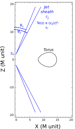
Figure 1: Scheme of the torus-jet model. The jet is parametrized by the angles $\theta_{1}$ and $\theta_{2}$ that describe the angular opening of the radiation-emitting sheath, by the base height $z_{b}$, the constant Lorentz factor $\Gamma_{j}$, and the temperature power-law index $s_{T}$. The jet is symmetrical with respect to the equatorial plane, and axisymmetric.

The emitting region is assumed to be defined by a thin layer in between two conical surfaces defined by the angles $\theta_{1}$ and $\theta_{2}$, and truncated at the jet base height $z_{b}$. The bulk Lorentz factor, as measured by the zero-angular-momentum observer (ZAMO), is assumed constant at $\Gamma_{j}$. The acceleration zone is thus discarded in this simple model.

Following Davelaar et al. (2018) we consider a population of electrons, at any point inside the jet sheath, satisfying a $\kappa$-distribution

$$n_{e}^{\mathrm{\kappa-distrib}}(\gamma)=N\,\gamma(\gamma^{2}-1)^{1/2}\left(1+\frac{\gamma-1}{\kappa\theta_{e}}\right)^{-(\kappa+1)}$$ (4)

where $N$ is a normalization factor depending on the averaged electron number density in the jet, $\langle n_{e}\rangle^{\mathrm{J}}$, and the dimensionless temperature $\theta_{e}$ ($N$ is defined by $\int_{\gamma}n_{e}^{\mathrm{\kappa-distrib}}(\gamma)\mathrm{d}\gamma=\langle n_{e}\rangle^{\mathrm{J}}$), $\gamma$ is the Lorentz factor of the electrons, and $\kappa$ is a parameter. This distribution smoothly connects a thermal distribution for small electron Lorentz factor, to a power-law distribution with power-law index $p=\kappa-1$ at high electron Lorentz factor. See Fig. 1 of Pandya et al. (2016) for an illustration of this distribution (note that the thermal/power-law transition takes place close to the peak of the distribution; this is different from the thermal+power-law-tail spectrum of the hard state of Cygnus X-1 as discussed in McConnell et al. 2002).

The averaged electron number density varies with the altitude $z$. By the conservation of mass, this quantity must scale as $\rho(z)^{-2}$ so that we can write

$$\langle n_{e}\rangle^{\mathrm{J}}(z)=\langle n_{e}\rangle^{\mathrm{J\;base}}\,\frac{\rho(z_{b})^{2}}{\rho(z)^{2}}$$ (5)

where $\langle n_{e}\rangle^{\mathrm{J\;base}}$ is the electron number density at the base of the jet, which is a parameter of the model. To obtain this expression, we assume that the jet matter flows across surfaces of area $\propto\rho(z)^{2}$, meaning that we consider the full jet (spine+sheath) for the mass conservation, while we consider only the sheath for the emission. This is reasonable given that the number density in the spine is typically extremely low (Mościbrodzka & Falcke 2013).

The magnetic field magnitude follows from the specification of the magnetization parameter $\sigma$

$$\frac{B(z)^{2}}{4\pi}=\sigma\,m_{p}c^{2}\,\langle n_{e}\rangle^{\mathrm{J}}(z)$$ (6)

where $m_{p}$ is the proton mass. This means that the magnetic field will approximately scale like $1/r$.

The temperature of the electrons at the base of the jet, $T_{e}^{\mathrm{J\;base}}$, is a parameter of the model. We are then free to prescribe the profile of temperature with altitude. To justify our choice, let us remind that the standard isothermal jet model of Blandford & Königl (1979) produces a flat radio spectrum. For Sgr A*, Fig. 2 shows that the radio spectral data are not exactly flat: more flux is needed at higher frequencies (closer to the black hole), rather than at lower frequencies (further from the black hole). To obtain this behavior, we consider a non-isothermal model such that the temperature decreases

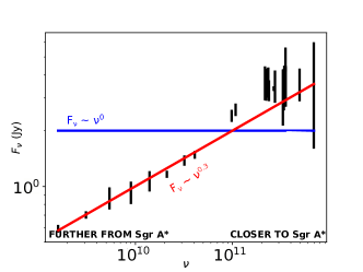
Figure 2: The radio to millimeter spectrum of Sgr A* (black error bars; see Fig. 3 for references). The blue horizontal line shows the spectrum produced by an isothermal jet. The red line shows what is needed by the data.

with altitude following a power law

$$T_{e}^{\mathrm{J}}(z)=T_{e}^{\mathrm{J\;base}}\,\left(\frac{z_{b}}{z}\right)^{s_{T}}$$ (7)

where the temperature slope $s_{T}$ is a parameter. A value of $s_{T}=0$ would lead to an isothermal jet model close to Blandford & Königl (1979). We will consider values $0\leq s_{T}\leq 1$.

Our goal is to ray trace this model so we need to properly define the 4-velocity of the ejected gas at every points inside the jet, which will be needed to compute redshift effects during the ray tracing. The Lorentz factor $\Gamma_{j}$ being measured by the ZAMO having 4-velocity $\mathbf{u_{\mathrm{ZAMO}}}$, the 4-velocity of the jet particles can be written

$$\mathbf{u_{\mathrm{jet}}}=\Gamma_{j}\left(\mathbf{u_{\mathrm{ZAMO}}}+\mathbf{V}\right)$$ (8)

where $\mathbf{V}=(V^{t}=0,V^{r},V^{\theta},V^{\varphi}=0)$ is the jet velocity as measured by the ZAMO, and can be seen as the usual 3-velocity of the jet. Here, it has only $2$ non-zero components due to the axisymmetry. This jet velocity can be written easily at the external and internal sheath surfaces (respectively defined by the angles $\theta_{1}$ and $\theta_{2}$)

$$\mathbf{V}=V\left(\sin\theta_{k}\,\mathbf{e_{\rho}}+\cos\theta_{k}\,\mathbf{e}_{z}\right)$$ (9)

where $\mathbf{e_{\rho}}$ and $\mathbf{e_{z}}$ are unit vectors, $V=\sqrt{\Gamma_{j}^{2}-1}/\Gamma_{j}$ is the jet velocity in units of the speed of light, and the angle $\theta_{k}$ can be $\theta_{1}$ or $\theta_{2}$. The velocity at any point inside the sheath, defined by an angle with the $\mathbf{e}_{z}$ direction equal to $\theta_{2}<\theta<\theta_{1}$, can then be easily interpolated linearly between $\theta_{1}$ and $\theta_{2}$.

The synchrotron emission and absorption coefficients for the $\kappa$-distribution electrons are taken from Pandya et al. (2016), in their Eq. 35-41, averaged over the angle $\theta_{B}$ between the magnetic field direction and the direction of emission. The low- and high-frequency dimensionless emission coefficients, as well as the bridging emission coefficient, read

$$\mathcal{J}_{\nu}^{\mathrm{low}} = X_{\kappa}^{1/3}\sin\theta_{B}\,\frac{4\pi\,\Gamma(\kappa-4/3)}{3^{7/3}\,\Gamma(\kappa-2)},$$ (10)

$$\mathcal{J}_{\nu}^{\mathrm{high}} = X_{\kappa}^{-(\kappa-2)/2}\sin\theta_{B}\,3^{(\kappa-1)/2}$$

$$\times\frac{(\kappa-2)(\kappa-1)}{4}\,\Gamma(\kappa/4-1/3)\Gamma(\kappa/4+4/3),$$

$$j_{\nu}^{\mathrm{\kappa-distrib}} = \frac{\langle n_{e}\rangle^{\mathrm{J}}\,e^{2}\,\nu_{c}}{c}\,\left[\left(\mathcal{J}_{\nu}^{\mathrm{low}}\right)^{-x_{j}}+\left(\mathcal{J}_{\nu}^{\mathrm{high}}\right)^{-x_{j}}\right]^{-1/x_{j}}$$

where $X_{\kappa}=\nu/(\nu_{c}(\theta_{e}\kappa)^{2}\sin\theta_{B})$, $\Gamma$ is the gamma function, and $x_{j}=3\,\kappa^{-3/2}$. This fit is correct for $3\leq\kappa\leq 7$. Similarly, the absorption coefficient is given by

$$\mathcal{A}_{\nu}^{\mathrm{low}} = X_{\kappa}^{-2/3}\,3^{1/6}\,\frac{10}{41}$$

$$\times\frac{2\pi}{(\theta_{e}\kappa)^{10/3-\kappa}}\,\frac{(\kappa-2)(\kappa-1)\kappa}{3\kappa-1}\,\Gamma(5/3)$$

$$\times_{2}F_{1}(\kappa-1/3,\kappa+1;\kappa+2/3;-\kappa\theta_{e}),$$

$$\mathcal{A}_{\nu}^{\mathrm{high}} = X_{\kappa}^{-(1+\kappa)/2}\,\frac{\pi^{3/2}}{3}\,\frac{(\kappa-2)(\kappa-1)\kappa}{(\theta_{e}\kappa)^{3}}$$

$$\times\left[\frac{2\,\Gamma(2+\kappa/2)}{2+\kappa}-1\right]\,\left[\left(\frac{3}{\kappa}\right)^{19/4}+\frac{3}{5}\right],$$

$$\alpha_{\nu}^{\mathrm{\kappa-distrib}} = \frac{\langle n_{e}\rangle^{\mathrm{J}}\,e^{2}}{\nu\,m_{e}\,c}\,\left[\left(\mathcal{A}_{\nu}^{\mathrm{low}}\right)^{-x_{\alpha}}+\left(\mathcal{A}_{\nu}^{\mathrm{high}}\right)^{-x_{\alpha}}\right]^{-1/x_{\alpha}}$$

where $x_{\alpha}=(-7/4+8\kappa/5)^{-43/50}$, and ${}_{2}F_{1}(a,b;c;z)$ is the Gauss hypergeometric function. This function is computed by means of the implementation of Michel & Stoitsov (2008).

3 Spectra and images of the quiescent Sgr A*

We transport the synchrotron emission from the torus and jet described above by means of the general-relativistic open-source ray tracing code Gyoto  (Vincent et al. 2011). Null geodesics are traced backwards in coordinate time, from the distant observer towards the black hole. The radiative transfer equation is integrated inside the torus and jet. We have made a resolution study to check that our choice of the technical ray-tracing parameters, like the observer’s screen resolution and field of view, ensures a precision of $<5\%$ on the spectra. This study is briefly summarized in Appendix A.

Our torus+jet model is described by the set of $19$ parameters described in Table 1.

Table 1: Torus+jet model best-fit parameters at inclination $i=20^{\circ}$. The value of the parameter is given in bold if it is fitted. Otherwise, the value is fixed. See text for the definition of the parameters. For the temperatures, we also give the dimensionless electron temperature $\Theta_{e}=kT_{e}/(m_{e}c^{2})$. Note that the magnetic/gas pressure ratio, defined by Eq. 6, is different from the standard plasma-$\beta$ parameter. The latter is discussed in Eq. 12. We note that the total mass of the torus is of $\approx 10^{-10}\,M_{\odot}$.

parameter		value
Black hole
mass ($M_{\odot}$)	$M$	$4.1\times 10^{6}$
distance (kpc)	$D$	$8.1\leavevmode\nobreak\$
spin	$a$	$0$
inclination (∘)	$i$	$20$
Torus
angular momentum ($GM/c^{3}$)	$\ell$	$4$
inner radius ($GM/c^{2}$)	$r_{\mathrm{in}}$	$\boldsymbol{8}$
polytropic index	$k$	$5/3$
central density ($\mathrm{cm}^{-3}$)	$\langle n_{e}\rangle^{\mathrm{T\;cen}}$	$\boldsymbol{1.2\times 10^{9}}$
central temperature (K)	$T_{e}^{\mathrm{T\;cen}}$	$\boldsymbol{7\times 10^{9}}$
	$\Theta_{e}^{\mathrm{T\;cen}}$	1.2
magnetization parameter	$\sigma^{\mathrm{T}}$	$0.002$
Jet
inner opening angle (∘)	$\theta_{1}$	$20$
outer opening angle (∘)	$\theta_{2}$	$\theta_{1}+3.5$
jet base height ($GM/c^{2}$)	$z_{b}$	$2$
bulk Lorentz factor	$\Gamma_{j}$	$1.15$
base number density ($\mathrm{cm}^{-3}$)	$\langle n_{e}\rangle^{\mathrm{J\;base}}$	$\boldsymbol{5\times 10^{7}}$
base temperature (K)	$T_{e}^{\mathrm{J\;base}}$	$\boldsymbol{3\times 10^{10}}$
	$\Theta_{e}^{\mathrm{J\;base}}$	5.
temperature slope	$s_{T}$	$\mathbf{0.21}$
$\kappa$-distribution index	$\kappa$	$\mathbf{5.5}$
magnetization parameter	$\sigma^{\mathrm{J}}$	$0.01$

A complete study of the parameter space would be very long in terms of computing time, and not particularly interesting as we may converge to solutions that are unlikely to occur in reality. As a consequence, we prefer to rather investigate the parameter space in a rather small region around the best-fit values of the recent articles by Mościbrodzka & Falcke (2013); Davelaar et al. (2018). Moreover, we will simply fix those parameters that are already rather well constrained, or that are fully degenerate with other parameters. In this latter case, we will choose values close to the best-fit numerical solutions available. The black hole mass and distance are fixed following Gravity Collaboration et al. (2018a). We consider two illustrative values for the inclination (angle between the normal to the equatorial plane and the line of sight): either close to face-on, $i=20^{\circ}$, which is in agreement with the recent constraint from Gravity Collaboration et al. (2018b), or close to edge-on, $i=70^{\circ}$. As already mentioned, the spin is likely to have a small impact on the results and is arbitrarily fixed to $a=0$. The torus constant angular momentum scales the location of the torus center (where density and temperature are maximum), which we decide to fix arbitrarily at $r_{\mathrm{cen}}\approx 10\,GM/c^{2}$, leading to $\ell=4\,GM/c^{3}$. The polytropic index is fixed to $k=5/3$. The magnetization parameters are fixed to $\sigma^{\mathrm{J}}=0.01$ in the jet and $\sigma^{\mathrm{T}}=0.002$ in the torus. These values were chosen by fixing the torus and jet number densities to the best-fit values of Davelaar et al. (2018) and imposing to find similar values for the magnetic field. The jet inner and outer opening angles are fixed to values similar to that describing the jet sheath of Mościbrodzka & Falcke (2013). The opening angle of the jet has an overall increasing/decreasing effect on the spectrum that would be fully degenerate with the base number density. The jet base height is arbitrarily fixed to $2\,GM/c^{2}$ (coinciding with the Schwarzschild event horizon), while the bulk Lorentz factor is fixed to $\Gamma_{j}=1.15$, approximately corresponding to the Keplerian velocity at the Schwarzschild innermost stable circular orbit. The other $7$ parameters (the central density, central temperature and inner radius of the torus, the base density and temperature of the jet, the temperature slope, and the $\kappa$ index) are let free and are fitted to the spectral observations. The temperature slope and $\kappa$ index have a strong impact on the spectrum slope in the radio and infrared region, respectively, so that their values can be rather easily constrained. There are thus only $5$ parameters that we scan in detail to find our best fits.

As we will see in Fig. 3, the torus has a non-negligible impact on the spectrum only in the millimeter band. As a consequence, we have divided our parameter space scanning into two easier sub-tasks: first we fit a pure jet (with no torus) to the radio and infrared spectral data (removing the millimeter peak). Then we fix the jet parameters at their values at the best fit of this search and fit the torus parameters by fitting the full spectrum (from radio to infrared). This allows to decrease the dimensions of the parameter space and thus save computing time. We thus considered one 2D grid (density, temperature) for the jet, and one separate 3D grid (density, temperature, inner radius) for the torus. We note that we fit our model to the spectral data only. The validity of the constraints on the radio image size and infrared spectral index are then checked a posteriori.

The left panel of Fig. 3 shows the best-fit spectra obtained for the two values of inclination considered here, $i=20^{\circ}$ and $i=70^{\circ}$.

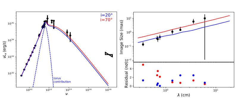
Figure 3: Left: Best-fit torus+jet quiescent spectrum at $i=20^{\circ}$ (blue, $\chi^{2}_{\mathrm{red}}=0.54$, with the torus-only contribution dashed; it is very similar for both inclinations so we represent only the $i=20^{\circ}$ case) and $i=70^{\circ}$ (red, $\chi^{2}_{\mathrm{red}}=0.87$). The data are taken from Bower et al. (2015, all radio data except the 4 points described just after), Brinkerink et al. (2015, for the 2 points around 100 GHz),  Liu et al. (2016, for the 492 GHz point), Marrone et al. (2006, for the 690 GHz point), von Fellenberg et al. (2018, for the far infrared upper limits), Witzel et al. (2018, for the mid infrared data), and Baganoff et al. (2001, for the X-ray bow-tie). Note that the X-ray data is not fitted as we do not take into account bremsstrahlung nor Comptonized emission. Right: corresponding image major axis at radio wavelengths (upper panel), with data from Bower et al. (2006). The lower panel shows the residual in units of $\sigma$.

The fits are extremely good, with reduced chi-squared $\approx 1$ for both inclinations. The best-fit parameters are listed in Table 1 for the $i=20^{\circ}$ case. Those of the $i=70^{\circ}$ case are the same except for the following: $r_{\mathrm{in}}=6\,GM/c^{2}$, $\langle n_{e}\rangle^{\mathrm{T\;cen}}=8.7\times 10^{8}\,\mathrm{cm}^{-3}$, $T_{e}^{\mathrm{T\;cen}}=6\times 10^{9}$ K, $\langle n_{e}\rangle^{\mathrm{J\;base}}=7.5\times 10^{7}\,\mathrm{cm}^{-3}$. It is interesting to compare the jet-base and torus-center values of the number density, temperature and magnetic field to the best-fit GRMHD simulation of Davelaar et al. (2018). We checked that our best-fit values are within a maximum factor of $\approx 2.5$ from that of these authors. This is a rather strong argument in favor of the robustness of both methods. It also shows that our much simpler analytic model does capture the essential aspects of the physics at play. We also note the striking similarity between our best-fit non-thermal spectra and that of Yuan et al. (2003), developed for the very different context of RIAFs (see e.g. the recently updated Fig. 19 of Witzel et al. 2018). We consider that such comparisons are strong arguments in favor of the robustness of the simulations of Sgr A* accretion flow.

At this point, it is interesting to compute what is our best-fit plasma $\beta$ parameter, as defined in the standard way of the ratio between the thermal to magnetic pressure ratio. We find

$$\beta=8\pi\,\frac{\langle n_{e}\rangle\,k\,T_{e}}{B^{2}}\approx 0.6$$ (12)

which is valid both at the center of the torus and at the base of the jet. Our plasma is thus close to be fully magnetized (i.e. to $\beta=1$). This value is comparable to the inner disk $\beta$ of Ressler et al. (2017), as reported in their Fig. 1, lower-left panel.

Based on the recent detailed analysis of the infrared statistical properties of Sgr A* by Witzel et al. (2018), we can also discuss the value of our predicted infrared spectral index. Here, we define this index as the factor $\alpha$ such that the specific infrared flux follows $F_{\nu}\propto\nu^{-\alpha}$. This parameter is easily related to the $\kappa$ index of our electron distribution through $\alpha=(\kappa-2)/2$. With our best-fit value of $\kappa=5.5$, the predicted spectral index of our model is thus $\alpha^{\mathrm{predict}}=1.75$. The (dereddened) $2.2\,\mu$m luminosity of our $i=20^{\circ}$ best-fit model reaches $\nu L_{\nu}=1.06\times 10^{34}$ erg/s. Using Table 6 of Witzel et al. (2018), which gives the relation between dereddened and non-dereddened fluxes of Sgr A*, this translates to a non-dereddened flux of order $0.1$ mJy. Using now Fig. 17 of Witzel et al. (2018), which gives the K-band spectral index as a function of the non-dereddened flux, this translates to a spectral index of the order of $\alpha^{\mathrm{obs}}=1.8$, so very close to our predicted value. The slightly higher flux value at $i=70^{\circ}$ leads to similar conclusions. Thus, our best-fit models are coherent with the quiescent constraints on Sgr A*’s spectral index.

The third and final observable that we can use are the intrinsic radio sizes of Sgr A*. The right panel of Fig. 3 shows the predicted major axis size of our best-fit models for both inclinations, compared to the data of Bower et al. (2006). The major axis of the image is computed from the image central moments. We briefly remind this formalism in Appendix B. The right panel of Fig. 3 shows that our $i=20^{\circ}$ best-fit model is always at $<2.5\sigma$ from the $0.35$ to $6$ cm data of Bower et al. (2006), which gives a reasonable agreement over this range. However, our model predicts that the size evolves like $\lambda^{\gamma}$, where $\gamma\approx 0.8$, which is too shallow with respect to the constraint of Bower et al. (2006), who find that $\gamma^{\mathrm{obs}}\approx 1.6$. This leads our model to overpredicting the size of the image at lower wavelengths, as we will see below. We note that the centimeter-size behavior of our model is very similar to that depicted in Fig. 9 of Davelaar et al. (2018), again showing the ability of our simple description to lead to the same conclusions as the most sophisticated GRMHD simulations to date. Let us stress that the slope of the curve on the righ panel of Fig. 3 is only weakly dependent on the jet parameters. Davelaar et al. (2018) and Chael et al. (2018) have shown that the size of the cm emitting region is sensitive to the electron distribution function, so that the shallow slope that we get might be linked to our choice of purely $\kappa$-distribution electrons.

Doeleman et al. (2008) have given a constraint of the intrinsic diameter of Sgr A* at $1.3$ mm of $37^{+16}_{-10}\,\mu$as ($3\sigma$), based on a Gaussian fit. It is thus particularly interesting to examine the prediction of our model at this specific EHT wavelength. Fig. 4 shows the $1.3$ mm best-fit image of our model for both inclinations.

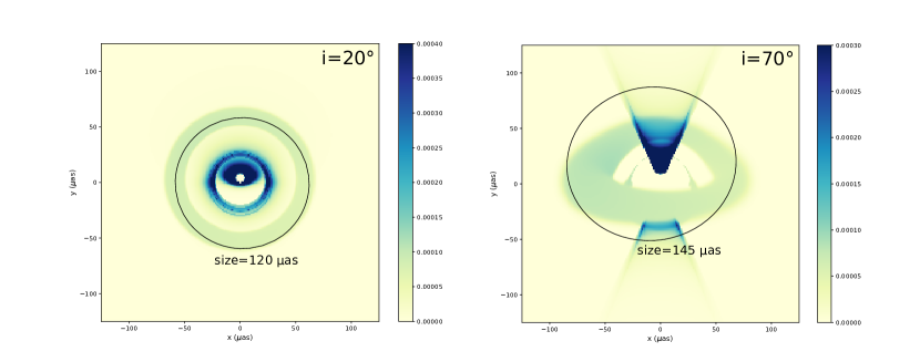
Figure 4: Best-fit torus+jet image at $1.3$ mm, as seen at inclination $i=20^{\circ}$ (left) and $i=70^{\circ}$ (right). The color bar is different for the two images to optimize the readability of each panel. It gives the value of the specific intensity in cgs units. The color hue is somewhat saturated to make it easier to see the fainter torus. As a consequence, the maximum value of the specific intensity is somewhat higher than the highest number of the color bars: $0.0015$ for the left panel, and $0.001$ for the right panel, in cgs units. The black ellipses are obtained by deriving the central moments of the images (see text for details) and give an estimate of the size of the emitting region, which is written explicitly in each panel.

It shows that our predicted $1.3$ mm size (as computed from image moments) is larger by a factor of $\approx 3$ at $i=20^{\circ}$ and $\approx 4$ at $i=70^{\circ}$, as compared to the Doeleman et al. (2008) constraint. This is mainly due to the presence of the faint extended torus, while our images also show prominent features at the $\lesssim 40\,\mu$as scale. The time-evolving GRMHD model of Davelaar et al. (2018) leads, here again, to very similar results. The size millimeter constraint reported above is valid assuming a circular Gaussian model for the source. A thick-ring model leads to an outer diameter intrinsic source size of $\approx 80\,\mu$as, so a factor $\approx 1.5$ smaller than our face-on prediction. The constraint of Doeleman et al. (2008) is thus only the first word on a nascent topic. In particular, this constraint is only valid in the projected direction of the baseline on sky, so that a complex geometry (like we have here with a thick disk and a jet), with an intrinsic size varying a lot with the angle on sky, might be too broadly described by this single number only. Therefore, we consider that our $1.3$ mm flux repartition is in reasonable agreement with the data. It is likely that the near-future EHT data will allow to constrain more precisely the geometry of the inner accretion flow, allowing to further refine the modeling part.

Fig. 4 shows that the $1.3$ mm image is due to a mix of contributions due to the torus and the jet. At radio wavelengths ($<10^{11}$ Hz), the jet completely dominates the spectrum, as emission primarily comes from large scales. Our model is also fully dominated by the jet for near infrared frequencies and above, as illustrated in Fig. 5, which shows the best-fit $2.2\,\mu$m images at both inclinations.

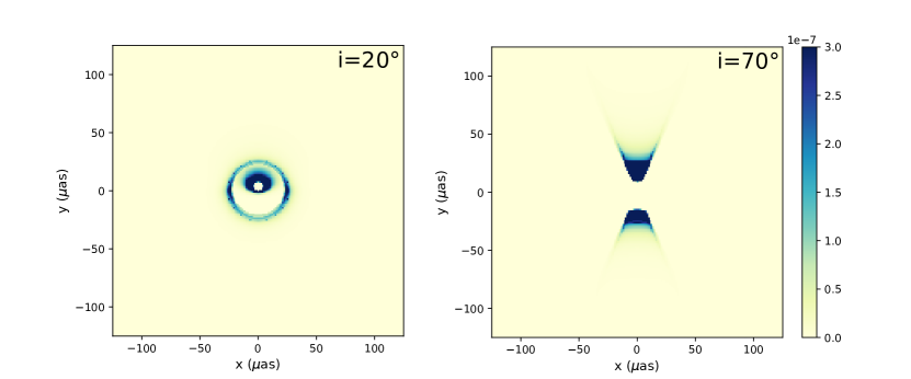
Figure 5: Best-fit torus+jet image at $2.2\,\mu$m, as seen at inclination $i=20^{\circ}$ (left) and $i=70^{\circ}$ (right). The color bar is common to both panels and gives the values of specific intensity in cgs units. As in Fig. 4, the color hue is somewhat saturated for better visualization.

This feature is in reasonable agreement with the near infrared images of Davelaar et al. (2018). However, this disagrees with the results of Ressler et al. (2017) who find that the disk dominates at all frequencies above the millimeter peak. This difference is certainly due to the different electron temperatures in the various models. In particular, Ressler et al. (2017) report hot spots of high electron temperature in the disk, that are obviously not present in our simple setup. These hot spots lead to a high near-infrared flux, which would not agree with the faintest quiescent level of Sgr A*.

Although the right panel of Fig. 5, showing the edge-on ray-traced image of a jet, is easy to interpret, it is likely that the left panel, showing the same scenery from a face-on view, is not so. Fig. 6 tries to explain this image, showing that the annular structure

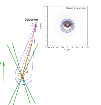
Figure 6: The green contours show a scheme of the jet sheath on both parts ($z>0$ and $z<0$) of the black hole. The observer is at $i=20^{\circ}$ at the top of the figure, with the observation screen represented at the top right. It is identical to the left panel of Fig. 5. Two regions are highlighted in red and blue. The red part is the primary image of the regions close to the $z>0$ base of the jet. Three examples of geodesics, ray-traced backwards in time from the observer’s screen, A, B, and C, are represented on the scheme, all of them ending their trajectory inside the black hole. Their end points on the observer’s screen are labeled. Geodesic C carries more flux, because it has visited regions very close to the base of the jet. While geodesic B, falling (backwards) straight into the black hole, carries no flux. The toroidal blue region on the observer’s screen is the secondary image of the jet, due to photons that are strongly bent in the regions close to the $z<0$ base of the jet, before reaching the far-away observer. Two such strongly-bent geodesics are depicted in blue on the scheme. This structure can thus be seen as the Einstein ring of the $z<0$ base of the jet.

is actually the Einstein ring of the $z<0$ base of the jet.

4 Reconstructing synthetic data with the EHT array

An important question to ask is whether salient features of Sgr A* near-horizon emission region, that we are parametrizing with analytic geometric models, could actually be observed by an instrument such as the EHT. The question concerns not only the instrument resolution, but also inherent limitations of the imaging from sparsely sampled Fourier domain data and utilizing a strongly inhomogeneous array of telescopes, both being traits of VLBI in general and EHT in particular. One of the limitations is a low dynamic range of VLBI synthesis images, see, e.g., Braun (2013). For a multicomponent source this could result in the inability of the EHT observations to reliably detect a weaker-flux component, such as a faint torus in the presence of a bright jet.

We investigate this issue by generating synthetic EHT observations of the images shown in Fig. 4 and subsequently attempting to reconstruct the images from sparsely sampled data. Synthetic observations and image reconstructions are generated using the freely available eht-imaging library . A Maximum Entropy Method (MEM), implemented in eht-imaging, was used for the image reconstruction, see Chael et al. (2016). The simulated observations fold in characteristic sensitivities of the EHT telescopes, and effects such as thermal noise contamination, rapid atmospheric phase variation, and dependence of sensitivity on source elevation. The EHT 2017 array was used, with optimal coverage in the Fourier domain. A static source model (i.e., single image) was assumed, which is a big simplification, as time variability on timescales as short as minutes is expected for Sgr A*. No mitigation of scattering, subdominant for $1.3$ mm wavelength, was employed.

EHT reconstruction results are shown in Fig. 7. They show that the salient features of the models persist in the reconstructed images. In particular, a wide region of weak emission, corresponding to the faint torus, is present in the reconstructed images. This successful reconstruction of the model images allows us to hope that similar features of the realistic Sgr A* accretion/ejection flow could be successfully revealed in EHT images. If so, simple geometric models such as ours could help interpreting future data and extracting relevant parameters, such as, in the present case, the inclination angle. Fig. 7 indeed shows that the reconstructed image is clearly dependent on this important parameter.

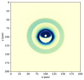
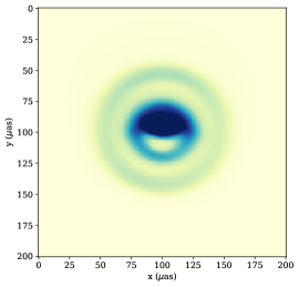
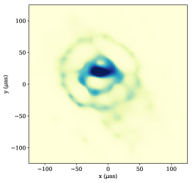
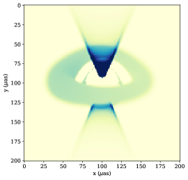
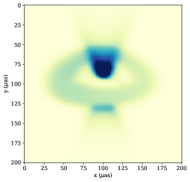
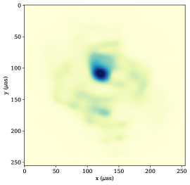
Figure 7: Example of model images reconstruction with the synthetic EHT array. For display purposes colormaps saturates at 0.001 Jy/px. Left column: original synthetic images generated with our model (same as Fig. 4). Middle column: model images as processed by the interstellar scattering screen (Johnson et al. 2018). Right column: MEM reconstruction of images, observed by a synthetic EHT 2017 array (Chael et al. 2016). Fitting elliptical Gaussian component to images we find characteristic size [major axis, minor axis] of [97,72] $\mu$as for the top row image and [100,89] $\mu$as for the bottom row image.

5 Conclusion and perspectives

We present here a simple analytic model of the quiescent-state emission of Sgr A*, made of the combination of a compact torus and a large-scale jet sheath. Our model allows to fit very well the multi-wavelength spectral data of Sgr A*, as illustrated in the left panel of Fig. 3. The size of the radio/millimeter emitting region is in reasonable agreement with observed constraints, as illustrated in the right panel of Fig. 3 and in the discussion accompanying Fig. 4. Our Fig. 7 demonstrates that salient disk/jet features of our model images persist when synthetic data are ’observed’ and reconstructed using a numerical model of the EHT array, and that these features are sensitive to inclination.

It is interesting that our model, inspired by the recent work of Davelaar et al. (2018), leads to best-fit parameters very close to that found in the GRMHD simulations of these authors. We believe that this is a nice illustration of the interest of simple analytic models: they are able to reproduce the outputs of costly numerical simulations. It is also interesting that our spectral prediction is indistinguishable from the predictions of Yuan et al. (2003), who use a different analytic description of the surroundings of Sgr A*. This is a good argument that the theoretical descriptions of Sgr A* are robust in their predictions.

We consider that our model is a practical testbed to study various aspects of the physics of Sgr A*. We hope that this model can be useful for other authors, and describe all steps necessary to reproduce our results in Appendix C. In the near future, we aim at using this model to analyze and interpret the data from GRAVITY, EHT and possibly other millimeter-range VLBI observations.

Appendix A Resolution study

The emitting part of the jet in the radio range can extend to large distances, imposing to consider a large field of view for the ray tracing computation. Here, we investigate the resolution of the Gyoto screen (i.e. the number of pixels along one dimension, labeled $N$) needed to obtain a precise value of the observed flux. We want to determine the optimal pair of field of view $F$ and resolution $N$.

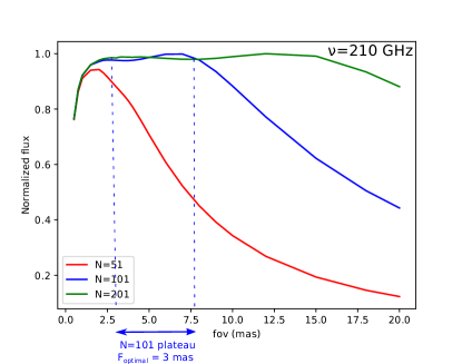
Figure 8: Evolution of the normalized ray-traced flux at $\nu=210$ GHz with increasing field of view for $3$ values of screen resolution, $N=51$ (red), $N=101$ (blue), and $N=201$ (green). The optimal value of field of view for a given resolution is the beginning of the plateau-phase of the curve (see text for details). The plateaus of the $N=101$ and $N=201$ curves are identical to within $0.1\%$, which shows that $N=101$ is the smallest resolution ensuring accurate flux values, associated to $F=3$ mas.

To do so, we study the evolution of the normalized flux with the field of view, for various resolutions and for a set of wavelengths. The overall behavior of these curves is easy to understand. For a given resolution, if the field of view is too small, the predicted flux is also too small because a portion of the emitting region leaks out of the field of view. If the field of view is too big, the predicted flux will also be too small, because the emitting region is diluted (at the limit of a field of view $4\pi$ steradian, the emitting region would be so small that the image would be completely black, leading to zero flux). Thus the curve showing the evolution of the flux as a function of the field of view first increases with the field of view, then stabilizes to form a plateau, and finally decreases. We select our $(N,F)$ pairs by imposing that the plateaus of the curves corresponding to $N$ and to $2N$ are equal to within $<5\%$. For the minimal $N$ satisfying this condition, we choose the smallest value of $F$ within the plateau. A smaller $F$ will lead to a smaller computing time (because the region to trace is smaller), so that this is the optimal choice in terms of both precision and computing time. Fig. 8 illustrates this procedure for the particular case of $\nu=210$ GHz. This figure shows that the plateau fluxes corresponding to the $N=101$ and $N=201$ curves are equal to within $0.1\leavevmode\nobreak\ \%$, while the $N=51$ plateau is $6\%$ off and thus rejected. Table 2 gives the various $(N,F)$ used in this article as a function of the observed frequency.

Table 2: Pairs of resolution $N$ and corresponding field of view $F$ used for the $i=20^{\circ}$ simulations of Section 3.

$\nu$ (Hz)	$(N,F\mathrm{(mas)})$
$1.6\times 10^{9}$	$(101,30)$
$3.1\times 10^{9}$	$(101,15)$
$5.4\times 10^{9}$	$(101,10)$
$9\times 10^{9}$	$(101,5)$
$1.4\times 10^{10}$	$(101,5)$
$2.1\times 10^{10}$	$(101,3)$
$3.2\times 10^{10}$	$(101,3)$
$4.09\times 10^{10}$	$(101,2.5)$
$1.08\times 10^{11}$	$(201,1)$
$>1.1\times 10^{11}$	$(201,0.5)$

Appendix B Image moments

Let $I(x,y)$ be a 2D image labeled by a Cartesian grid $(x,y)$. The central moment of order $p+q$ of image $I$ is the quantity

$$\mu_{pq}=\sum_{x}\sum_{y}(x-\bar{x})^{p}(y-\bar{y})^{q}\,I(x,y)$$ (13)

where $(\bar{x},\bar{y})$ is the centroid of the $I(x,y)$ distribution, i.e.

$$\bar{x}=\frac{\sum_{x}\sum_{y}x\,I(x,y)}{\sum_{x}\sum_{y}I(x,y)}$$ (14)

and similarly for $\bar{y}$.

The major axis of the best-fitting ellipse adjusted to the distribution of $I(x,y)$ in the image is then given by (Birchfield 2018)

$$L=2\sqrt{2\,\frac{\mu_{20}+\mu_{02}+\sqrt{(\mu_{20}-\mu_{02})^{2}+4\mu_{11}^{2}}}{\mu_{00}}}$$ (15)

while the orientation of the ellipse with respect to the Cartesian grid $(x,y)$ is

$$\tan 2\theta=\frac{2\mu_{11}}{\mu_{20}-\mu_{02}}.$$ (16)

The size-fitting ellipses of Fig. 4 are computed using these formulas, as implemented in the cv2 Python package.

Appendix C Using Gyoto to generate spectra and images

The code developped for this paper is part of Gyoto 1.3.1 (Paumard et al. 2019, also available at https://github.com/gyoto/Gyoto/tree/1.3.1). Gyoto is packaged for Debian GNU/Linux and its derivatives including Ubuntu and this version will be part of the next version of these operating systems to be released in 2019. The installation steps are detailed in the file INSTALL.Gyoto.md (skipping section 0: the pre-compiled versions of Gyoto do not contain the very recent new developments presented in this article).

The input file Gyoto/doc/examples/example-jet.xml gives the jet-only best-fit model for the $i=20^{\circ}$ case discussed in Section 3. The file Gyoto/doc/examples/example-torusjet.xml gives the torus+jet best-fit model, i.e. the model used to generate the face-on spectrum and image of Fig. 3 and 4. The xml files provided have parameters such that they allow an accurate computation of the spectrum in the $10^{11}$ to $10^{18}$ Hz range. Lower frequencies need higher resolution and longer computing time, see Appendix A.

The Python scripts Gyoto/doc/examples/plot-Spectrum.py and Gyoto/doc/examples/plot-Image.py allow to straightforwardly generate spectra (together with the latest observed data) and images (together with the best-fitting image-moment ellipse), just as in our Fig. 3 and 4.

We thus provide all the software needed to obtain the results presented in this article.

Interested people are very welcome to contact the Gyoto developers at frederic.vincent@obspm.fr, thibaut.paumard@obspm.fr to get help.

References

- Alberdi et al. (1993) Alberdi, A., Lara, L., Marcaide, J. M., et al. 1993, A&A, 277, L1
- Baganoff et al. (2001) Baganoff, F. K., Bautz, M. W., Brandt, W. N., et al. 2001, Nature, 413, 45
- Bietenholz et al. (2000) Bietenholz, M. F., Bartel, N., & Rupen, M. P. 2000, ApJ, 532, 895
- Birchfield (2018) Birchfield, S. 2018, Image Processing and Analysis (CENGAGE Learning, Boston)
- Blandford & Königl (1979) Blandford, R. D. & Königl, A. 1979, ApJ, 232, 34
- Bower et al. (2006) Bower, G. C., Goss, W. M., Falcke, H., Backer, D. C., & Lithwick, Y. 2006, ApJ, 648, L127
- Bower et al. (2014) Bower, G. C., Markoff, S., Brunthaler, A., et al. 2014, ApJ, 790, 1
- Bower et al. (2015) Bower, G. C., Markoff, S., Dexter, J., et al. 2015, ApJ, 802, 69
- Braun (2013) Braun, R. 2013, A&A, 551, A91
- Brinkerink et al. (2015) Brinkerink, C. D., Falcke, H., Law, C. J., et al. 2015, A&A, 576, A41
- Broderick et al. (2016) Broderick, A. E., Fish, V. L., Johnson, M. D., et al. 2016, ApJ, 820, 137
- Chael et al. (2018) Chael, A., Rowan, M., Narayan, R., Johnson, M., & Sironi, L. 2018, MNRAS, 478, 5209
- Chael et al. (2016) Chael, A. A., Johnson, M. D., Narayan, R., et al. 2016, ApJ, 829, 11
- Davelaar et al. (2018) Davelaar, J., Mościbrodzka, M., Bronzwaer, T., & Falcke, H. 2018, A&A, 612, A34
- Dexter et al. (2010) Dexter, J., Agol, E., Fragile, P. C., & McKinney, J. C. 2010, ApJ, 717, 1092
- Dibi et al. (2012) Dibi, S., Drappeau, S., Fragile, P. C., Markoff, S., & Dexter, J. 2012, MNRAS, 426, 1928
- Dodds-Eden et al. (2011) Dodds-Eden, K., Gillessen, S., Fritz, T. K., et al. 2011, ApJ, 728, 37
- Doeleman et al. (2009) Doeleman, S., Agol, E., Backer, D., et al. 2009, in Astronomy, Vol. 2010, astro2010: The Astronomy and Astrophysics Decadal Survey, 68
- Doeleman et al. (2008) Doeleman, S. S., Weintroub, J., Rogers, A. E. E., et al. 2008, Nature, 455, 78
- Falcke et al. (1993) Falcke, H., Mannheim, K., & Biermann, P. L. 1993, A&A, 278, L1
- Falcke & Markoff (2000) Falcke, H. & Markoff, S. 2000, A&A, 362, 113
- Falcke et al. (2009) Falcke, H., Markoff, S., & Bower, G. C. 2009, A&A, 496, 77
- Falcke et al. (2000a) Falcke, H., Melia, F., & Agol, E. 2000a, ApJ, 528, L13
- Falcke et al. (2000b) Falcke, H., Nagar, N. M., Wilson, A. S., & Ulvestad, J. S. 2000b, ApJ, 542, 197
- Genzel et al. (2010) Genzel, R., Eisenhauer, F., & Gillessen, S. 2010, Reviews of Modern Physics, 82, 3121
- Ghez et al. (2008) Ghez, A. M., Salim, S., Weinberg, N. N., et al. 2008, ApJ, 689, 1044
- Gillessen et al. (2009) Gillessen, S., Eisenhauer, F., Trippe, S., et al. 2009, ApJ, 692, 1075
- Gravity Collaboration et al. (2017) Gravity Collaboration, Abuter, R., Accardo, M., et al. 2017, A&A, 602, A94
- Gravity Collaboration et al. (2018a) Gravity Collaboration, Abuter, R., Amorim, A., et al. 2018a, A&A, 615, L15
- Gravity Collaboration et al. (2018b) Gravity Collaboration, Abuter, R., Amorim, A., et al. 2018b, A&A, 618, L10
- Issaoun et al. (2019) Issaoun, S., Johnson, M. D., Blackburn, L., et al. 2019, ApJ, 871, 30
- Jiménez-Rosales & Dexter (2018) Jiménez-Rosales, A. & Dexter, J. 2018, MNRAS, 478, 1875
- Johnson (2016) Johnson, M. D. 2016, ApJ, 833, 74
- Johnson et al. (2018) Johnson, M. D., Narayan, R., Psaltis, D., et al. 2018, ApJ, 865, 104
- Komissarov (2006) Komissarov, S. S. 2006, MNRAS, 368, 993
- Lamy et al. (2018) Lamy, F., Gourgoulhon, E., Paumard, T., & Vincent, F. H. 2018, Classical and Quantum Gravity, 35, 115009
- Liu et al. (2016) Liu, H. B., Wright, M. C. H., Zhao, J.-H., et al. 2016, A&A, 593, A44
- Markoff et al. (2001) Markoff, S., Falcke, H., Yuan, F., & Biermann, P. L. 2001, A&A, 379, L13
- Marrone et al. (2006) Marrone, D. P., Moran, J. M., Zhao, J.-H., & Rao, R. 2006, Journal of Physics Conference Series, 54, 354
- McConnell et al. (2002) McConnell, M. L., Zdziarski, A. A., Bennett, K., et al. 2002, ApJ, 572, 984
- Michel & Stoitsov (2008) Michel, N. & Stoitsov, M. V. 2008, Computer Physics Communications, 178, 535
- Mościbrodzka & Falcke (2013) Mościbrodzka, M. & Falcke, H. 2013, A&A, 559, L3
- Mościbrodzka et al. (2009) Mościbrodzka, M., Gammie, C. F., Dolence, J. C., Shiokawa, H., & Leung, P. K. 2009, ApJ, 706, 497
- Narayan et al. (1995) Narayan, R., Yi, I., & Mahadevan, R. 1995, Nature, 374, 623
- Özel et al. (2000) Özel, F., Psaltis, D., & Narayan, R. 2000, ApJ, 541, 234
- Pandya et al. (2016) Pandya, A., Zhang, Z., Chandra, M., & Gammie, C. F. 2016, ApJ, 822, 34
- Paumard et al. (2019) Paumard, T., Vincent, F. H., Straub, O., & Lamy, F. 2019, Gyoto 1.3.1, https://doi.org/10.5281/zenodo.2547541
- Quataert (2002) Quataert, E. 2002, ApJ, 575, 855
- Rees (1982) Rees, M. J. 1982, in American Institute of Physics Conference Series, Vol. 83, The Galactic Center, ed. G. R. Riegler & R. D. Blandford, 166–176
- Ressler et al. (2017) Ressler, S. M., Tchekhovskoy, A., Quataert, E., & Gammie, C. F. 2017, MNRAS, 467, 3604
- Shcherbakov et al. (2012) Shcherbakov, R. V., Penna, R. F., & McKinney, J. C. 2012, ApJ, 755, 133
- Straub et al. (2012) Straub, O., Vincent, F. H., Abramowicz, M. A., Gourgoulhon, E., & Paumard, T. 2012, A&A, 543, A83
- Vincent et al. (2016a) Vincent, F. H., Gourgoulhon, E., Herdeiro, C., & Radu, E. 2016a, Phys. Rev. D, 94, 084045
- Vincent et al. (2016b) Vincent, F. H., Meliani, Z., Grandclément, P., Gourgoulhon, E., & Straub, O. 2016b, Classical and Quantum Gravity, 33, 105015
- Vincent et al. (2011) Vincent, F. H., Paumard, T., Gourgoulhon, E., & Perrin, G. 2011, Classical and Quantum Gravity, 28, 225011
- Vincent et al. (2015) Vincent, F. H., Yan, W., Straub, O., Zdziarski, A. A., & Abramowicz, M. A. 2015, A&A, 574, A48
- von Fellenberg et al. (2018) von Fellenberg, S. D., Gillessen, S., Graciá-Carpio, J., et al. 2018, ArXiv e-prints
- Wang et al. (2013) Wang, Q. D., Nowak, M. A., Markoff, S. B., et al. 2013, Science, 341, 981
- Wardziński & Zdziarski (2000) Wardziński, G. & Zdziarski, A. A. 2000, MNRAS, 314, 183
- Witzel et al. (2018) Witzel, G., Martinez, G., Hora, J., et al. 2018, ApJ, 863, 15
- Yuan et al. (2002) Yuan, F., Markoff, S., & Falcke, H. 2002, A&A, 383, 854
- Yuan & Narayan (2014) Yuan, F. & Narayan, R. 2014, ARA&A, 52, 529
- Yuan et al. (2003) Yuan, F., Quataert, E., & Narayan, R. 2003, ApJ, 598, 301