SpinDoctor: a MATLAB toolbox for diffusion MRI simulation

Abstract

The complex transverse water proton magnetization subject to diffusion-encoding magnetic field gradient pulses in a heterogeneous medium can be modeled by the multiple compartment Bloch-Torrey partial differential equation. Under the assumption of negligible water exchange between compartments, the time-dependent apparent diffusion coefficient can be directly computed from the solution of a diffusion equation subject to a time-dependent Neumann boundary condition.

This paper describes a publicly available MATLAB toolbox called SpinDoctor that can be used 1) to solve the Bloch-Torrey partial differential equation in order to simulate the diffusion magnetic resonance imaging signal; 2) to solve a diffusion partial differential equation to obtain directly the apparent diffusion coefficient; 3) to compare the simulated apparent diffusion coefficient with a short-time approximation formula.

The partial differential equations are solved by $P1$ finite elements combined with built-in MATLAB routines for solving ordinary differential equations. The finite element mesh generation is performed using an external package called Tetgen.

SpinDoctor provides built-in options of including 1) spherical cells with a nucleus; 2) cylindrical cells with a myelin layer; 3) an extra-cellular space enclosed either a) in a box or b) in a tight wrapping around the cells; 4) deformation of canonical cells by bending and twisting; 5) permeable membranes; Built-in diffusion-encoding pulse sequences include the Pulsed Gradient Spin Echo and the Oscillating Gradient Spin Echo.

We describe in detail how to use the SpinDoctor toolbox. We validate SpinDoctor simulations using reference signals computed by the Matrix Formalism method. We compare the accuracy and computational time of SpinDoctor simulations with Monte-Carlo simulations and show significant speed-up of SpinDoctor over Monte-Carlo simulations in complex geometries. We also illustrate several extensions of SpinDoctor functionalities, including the incorporation of $T_{2}$ relaxation, the simulation of non-standard diffusion-encoding sequences, as well as the use of externally generated geometrical meshes.

1 Introduction

Diffusion magnetic resonance imaging is an imaging modality that can be used to probe the tissue micro-structure by encoding the incohorent motion of water molecules with magnetic field gradient pulses. This motion during the diffusion-encoding time causes a signal attenuation from which the apparent diffusion coefficient , (and possibly higher order diffusion terms, can be calculated [1, 2, 3].

For unrestricted diffusion, the root of the mean squared displacement of molecules is given by $\bar{x}=\sqrt{2\,dim\,\sigma_{0}t}$, where $dim$ is the spatial dimension, $\sigma_{0}$ is the intrinsic diffusion coefficient, and $t$ is the diffusion time. In biological tissue, the diffusion is usually hindered or restricted (for example, by cell membranes) and the mean square displacement is smaller than in the case of unrestricted diffusion. This deviation from unrestricted diffusion can be used to infer information about the tissue micro-structure. The experimental parameters that can be varied include

1. the diffusion time (one can choose the parameters of the diffusion-encoding sequence, such as Pulsed Gradient Spin Echo [2] and Oscillating Gradient [4]).

2. the magnitude of the diffusion-encoding gradient (when the magnetic resonance imaging signal is acquired at low gradient magnitudes, the signal contains only information about the apparent diffusion coefficient, at higher values, Kurtosis imaging [5] becomes possible);

3. the direction of the diffusion-encoding gradient (many directions may be probed, as in high angular resolution diffusion imaging [6]).

Using diffusion magnetic resonance imaging to get tissue structural information in the mamalian brain has been the focus of much experimental and modeling work in recent years [7, 8, 9, 10, 11, 12, 13, 14]. The predominant approach up to now has been adding the diffusion magnetic resonance imaging signal from simple geometrical components and extracting model parameters of interest. Numerous biophysical models subdivide the tissue into compartments described by spheres, ellipsoids, cylinders, and the extra-cellular space [15, 16, 7, 8, 9, 11, 17, 18, 19, 12]. Some model parameters of interest include axon diameter and orientation, neurite density, dendrite structure, the volume fraction and size distribution of cylinder and sphere components and the effective diffusion coefficient or tensor of the extra-cellular space.

Numerical simulations can help deepen the understanding of the relationship between the cellular structure and the diffusion magnetic resonance imaging signal and lead to the formulation of appropriate models. They can be also used to investigate the effect of different pulse sequences and tissue features on the measured signal which can be used for the development, testing, and optimization of novel diffusion magnetic resonance imaging pulse sequences [20, 21, 22, 23].

Two main groups of approaches to the numerical simulation of diffusion magnetic resonance imaging are 1) using random walkers to mimic the diffusion process in a geometrical configuration; 2) solving the Bloch-Torrey PDE , which describes the evolution of the complex transverse water proton magnetization under the influence of diffusion-encoding magnetic field gradients pulses.

The first group is referred to as Monte-Carlo simulations in the literature and previous works include [24, 25, 26, 13, 27]. A GPU-based acceleration of Monte-Carlo simulation was proposed in [28, 29]. Some software packages using this approach include

1. Camino Diffusion MRI Toolkit developed at UCL (http://cmic.cs.ucl.ac.uk/camino/);

2. DIFSIM developed at UC San Diego (http://csci.ucsd.edu/projects/simulation.html);

3. Diffusion Microscopist Simulator [25] developed at Neurospin, CEA.

The second group relies on solving the Bloch-Torrey PDE in a geometrical configuration. In [30, 31, 32] a simplifying assumption called the narrow pulse approximation was used, where the pulse duration was assumed to be much smaller than the delay between pulses. This assumption allows the solution of the diffusion equation instead of the more complicated Bloch-Torrey PDE. More generally, numerical methods to solve the Bloch-Torrey PDE. with arbitrary temporal profiles have been proposed in [33, 34, 35, 36]. The computational domain is discretized either by a Cartesian grid [33, 37, 34] or finite elements [30, 31, 32, 35, 36]. The unstructured mesh of a finite element discretization appeared to be better than a Cartesian grid in both geometry description and signal approximation [35]. For time discretization, both explicit and implicit methods have been used. In [32] a second order implicit time-stepping method called the generalized $\alpha-$method was used to allow for high frequency energy dissipation. An adaptive explicit Runge-Kutta Chebyshev method of second order was used in [34, 35]. It has been theoretically proven that the Runge-Kutta Chebyshev method allows for a much larger time-step compared to the standard explicit Euler method [38]. There is an example showing that the Runge-Kutta Chebyshev method is faster than the implicit Euler method in [35]. The Crank-Nicolson method was used in [36] to also allow for second order convergence in time. The efficiency of diffusion magnetic resonance imaging simulations is also improved by either a high-performance FEM computing framework [39, 40] for large-scale simulations on supercomputers or a discretization on manifolds for thin-layer and thin-tube media [41].

In this paper, we present a MATLAB Toolbox called SpinDoctor that is a simulation pipeline going from the definition of a geometrical configuration through the numerical solution of the Bloch-Torrey PDE to the fitting of the apparent diffusion coefficient from the simulated signal. It also includes two other modules for calculating the apparent diffusion coefficient. The first module is a homogenized apparent diffusion coefficient mathematical model, which was obtained recently using homogenization techniques on the Bloch-Torrey PDE. In the homogenized model, the apparent diffusion coefficient of a geometrical configuration can be computed after solving a diffusion equation subject to a time-dependent Neumann boundary condition, under the assumption of negligible water exchange between compartments. The second module computes the short time approximation formula for the apparent diffusion coefficient. The short time approximation implemented in SpinDoctor includes a recent generalization of this formula to account for finite pulse duration in the pulsed gradient spin echo. Both of these two apparent diffusion coefficient calculations are sensitive to the diffusion-encoding gradient direction, unlike many previous works where the anisotropy is neglected in analytical model development.

In summary, SpinDoctor

1. solves the Bloch-Torrey PDE in three dimensions to obtain the diffusion magnetic resonance imaging signal;

2. robustly fits the diffusion magnetic resonance imaging signal to obtain the apparent diffusion coefficient;

3. solves the homogenized apparent diffusion coefficient model in three dimensions to obtain the apparent diffusion coefficient;

4. computes the short-time approximation of the apparent diffusion coefficient;

5. computes useful geometrical quantities such as the compartment volumes and surface areas;

6. allows permeable membranes for the Bloch-Torrey PDE (the homogenized apparent diffusion coefficient assumes negligible permeabilty).

7. displays the gradient-direction dependent apparent diffusion coefficient; in three dimensions using spherical harmonics interpolation;

SpinDoctor provides the following built-in functionalities:

1. placement of non-overlapping spherical cells (with an optional nucleus) of different radii close to each other;

2. placement of non-overlapping cylindrical cells (with an optional myelin layer) of different radii close to each other in a canonical configuration where they are parallel to the $z$-axis;

3. inclusion of an extra-cellular space that is enclosed either

   1. in a tight wrapping around the cells; or

   2. in a rectangular box;

4. deformation of the canonical configuration by bending and twisting;

Built-in diffusion-encoding pulse sequences include

1. the Pulsed Gradient Spin Echo ;

2. the Oscillating Gradient Spin Echo (cos- and sin- type gradients).

SpinDoctor uses the following methods:

1. it generates a good quality surface triangulation of the user specified geometrical configuration by calling built-in MATLAB computational geometry functions;

2. it creates a good quality tetrehedra finite elements mesh from the above surface triangulation by calling Tetgen [42], an external package (executable files are included in the Toolbox package);

3. it constructs finite element matrices for linear finite elements on tetrahedra (P1) using routines from [43];

4. it adds additional degrees of freedom on the compartment interfaces to allow permeability conditions for the Bloch-Torrey PDE using the formalism in [44];

5. it solves the semi-discretized FEM equations by calling built-in MATLAB routines for solving ordinary differential equations .

The SpinDoctor toolbox has been developed in the MATLAB R2017b and requires no additional MATLAB toolboxes. The toolbox is publicly available at:

https://github.com/jingrebeccali/SpinDoctor

Abbreviations frequently used in the text

MRI - magnetic resonance imaging

dMRI - diffusion magnetic resonance imaging

ADC - apparent diffusion coefficient

HADC - homogenized ADC

PGSE - pulsed gradient spin echo

OGSE - oscillating gradient

ECS - extra-cellular space

BTPDE - Bloch-Torrey partial differential equation

PDE - partial differential equation

ODE - ordinary differential equation

HARDI - high angular resolution diffusion imaging

STA - short time approximation

FE - finite elements

2 Theory

Suppose the user would like to simulate a geometrical configuration of cells with an optional myelin layer or a nucleus. If spins will be leaving the cells or if the user wants to simulate the extra-cellular space (ECS), then the ECS will enclose the geometrical shapes. Let $\Omega^{e}$ be the ECS, $\Omega^{in}_{i}$ the nucleus (or the axon) and $\Omega^{out}_{i}$ the cytoplasm (or the myelin layer) of the $i$th cell. We denote the interface between $\Omega^{in}_{i}$ and $\Omega^{out}_{i}$ by $\Gamma_{i}$ and the interface between $\Omega^{out}_{i}$ and $\Omega^{e}$ by $\Sigma_{i}$, finally the outside boundary of the ECS by $\Psi$.

2.1 Bloch-Torrey PDE

In diffusion MRI, a time-varying magnetic field gradient is applied to the tissue to encode water diffusion. Denoting the effective time profile of the diffusion-encoding magnetic field gradient by $f(t)$, and letting the vector ${\bm{g}}$ contain the amplitude and direction information of the magnetic field gradient, the complex transverse water proton magnetization in the rotating frame satisfies the Bloch-Torrey PDE:

$$\frac{\partial}{\partial t}{M^{in}_{i}({\bm{x}},t)} =-I\gamma f(t){\bm{g}}\cdot{\bm{x}}\,M^{in}_{i}({\bm{x}},t)+\nabla\cdot(\sigma^{in}\nabla M^{in}_{i}({\bm{x}},t)), {\bm{x}}\in\Omega^{in}_{i},$$ (1)

$$\frac{\partial}{\partial t}{M^{out}_{i}({\bm{x}},t)} =-I\gamma f(t){\bm{g}}\cdot{\bm{x}}\,M^{out}_{i}({\bm{x}},t)+\nabla\cdot(\sigma^{out}\nabla M^{out}_{i}({\bm{x}},t)),\; {\bm{x}}\in\Omega^{out}_{i},$$ (2)

$$\frac{\partial}{\partial t}{M^{e}({\bm{x}},t)} =-I\gamma f(t){\bm{g}}\cdot{\bm{x}}\,M^{e}({\bm{x}},t)+\nabla\cdot(\sigma^{e}\nabla M^{e}({\bm{x}},t)), {\bm{x}}\in\Omega^{e},$$ (3)

where $\gamma=2.67513\times 10^{8}\,\rm rad\,s^{-1}T^{-1}$ is the gyromagnetic ratio of the water proton, $I$ is the imaginary unit, $\sigma^{l}$ is the intrinsic diffusion coefficient in the compartment $\Omega^{l}_{i}$. The magnetization is a function of position ${\bm{x}}$ and time $t$, and depends on the diffusion gradient vector ${\bm{g}}$ and the time profile $f(t)$. We denote the restriction of the magnetization in $\Omega^{in}_{i}$ by $M^{in}_{i}$, and similarly for $M^{out}_{i}$ and $M^{e}$.

Some commonly used time profiles (diffusion-encoding sequences) are:

1. The pulsed-gradient spin echo (PGSE) [2] sequence, with two rectangular pulses of duration $\delta$, separated by a time interval $\Delta-\delta$, for which the profile $f(t)$ is

   $$f(t)=\begin{cases}1,\quad&t_{1}\leq t\leq t_{1}+\delta,\\ -1,\quad&t_{1}+\Delta<t\leq t_{1}+\Delta+\delta,\\ 0,\quad&\text{otherwise,}\end{cases}$$ (4)

   where $t_{1}$ is the starting time of the first gradient pulse with $t_{1}+\Delta>T_{E}/2$, $T_{E}$ is the echo time at which the signal is measured.

2. The oscillating gradient spin echo (OGSE) sequence [45, 4] was introduced to reach short diffusion times. An OGSE sequence usually consists of two oscillating pulses of duration $T$, each containing $n$ periods, hence the frequency is $\omega=n\frac{2\pi}{T}$, separated by a time interval $\tau-T$. For a cosine OGSE, the profile $f(t)$ is

   $$f(t)=\begin{cases}\cos{(n\frac{2\pi}{T}t)},\quad&t_{1}<t\leq t_{1}+T,\\ -\cos{(n\frac{2\pi}{T}(t-\tau))},\quad&\tau+t_{1}<t\leq t_{1}+\tau+T,\\ 0,\quad&\text{otherwise},\end{cases}$$ (5)

   where $\tau=T_{E}/2$.

The BTPDE needs to be supplemented by interface conditions. We recall the interface between $\Omega^{in}_{i}$ and $\Omega^{out}_{i}$ is $\Gamma_{i}$, the interface between $\Omega^{out}_{i}$ and $\Omega^{e}$ is $\Sigma_{i}$, and the outside boundary of the ECS is $\Psi$. The two interface conditions on $\Gamma_{i}$ are the flux continuity and a condition that incorporates a permeability coefficient $\kappa^{in,out}$ across $\Gamma_{i}$: :

$$\sigma^{in}\nabla M^{in}_{i}({\bm{x}},t)\cdot{\bm{n}}^{in}_{i} =-\sigma^{out}\nabla M^{out}_{i}({\bm{x}},t)\cdot{\bm{n}}^{out}_{i},\quad {\bm{x}}\in\Gamma_{i},$$

$$\sigma^{in}\nabla M^{in}_{i}({\bm{x}},t)\cdot{\bm{n}}^{in}_{i} =\kappa^{in,out}\Bigl{(}M^{out}_{i}({\bm{x}},t)-M^{in}_{i}({\bm{x}},t)\Bigl{)},\quad {\bm{x}}\in\Gamma_{i},$$

where ${\bm{n}}$ is the unit outward pointing normal vector. Similarly, between $\Omega^{out}_{i}$ and $\Omega^{e}$ we have

$$\sigma^{out}\nabla M^{out}_{i}({\bm{x}},t)\cdot{\bm{n}}^{out}_{i} =-\sigma^{e}\nabla M^{e}({\bm{x}},t)\cdot{\bm{n}}^{e},\quad {\bm{x}}\in\Sigma_{i},$$

$$\sigma^{out}\nabla M^{out}_{i}({\bm{x}},t)\cdot{\bm{n}}^{out}_{i} =\kappa^{out,e}\Bigl{(}M^{e}({\bm{x}},t)-M^{out}_{i}({\bm{x}},t)\Bigl{)},\quad {\bm{x}}\in\Sigma_{i}.$$

Finally, on the outer boundary of the ECS we have

$$0=\sigma^{e}\nabla M^{e}({\bm{x}},t)\cdot{\bm{n}}^{e},\quad{\bm{x}}\in\Psi.$$

The BTPDE also needs initial conditions:

$$M^{in}_{i}({\bm{x}},0)=\rho^{in},\quad M^{out}_{i}({\bm{x}},0)=\rho^{out},\quad M^{e}({\bm{x}},0)=\rho^{e}.$$

where $\rho$ is the initial spin density.

The dMRI signal is measured at echo time $t=T_{E}>\Delta+\delta$ for PGSE and $T_{E}>2\sigma$ for OGSE. This signal is the integral of $M({\bm{x}},T_{E})$:

$$S:=\int_{{\bm{x}}\in\bigcup\{\Omega^{in}_{i},\;\Omega^{out}_{i},\;\Omega^{e}\}}M({\bm{x}},T_{E})\;d{\bm{x}}.$$ (6)

In a dMRI experiment, the pulse sequence (time profile $f(t)$) is usually fixed, while ${\bm{g}}$ is varied in amplitude (and possibly also in direction). $S$ is usually plotted against a quantity called the $b$-value. The $b$-value depends on ${\bm{g}}$ and $f(t)$ and is defined as

$$b({\bm{g}})=\gamma^{2}\|{\bm{g}}\|^{2}\int_{0}^{T_{E}}du\left(\int_{0}^{u}f(s)ds\right)^{2}.$$

For PGSE, the b-value is [2]:

$$b({\bm{g}},\delta,\Delta)=\gamma^{2}\|{\bm{g}}\|^{2}\delta^{2}\left(\Delta-\delta/3\right).$$ (7)

For the cosine OGSE with integer number of periods $n$ in each of the two durations $\sigma$, the corresponding $b$-value is [33]:

$$b({\bm{g}},\sigma)=\gamma^{2}\|{\bm{g}}\|^{2}\frac{\sigma^{3}}{4n^{2}\pi^{2}}=\gamma^{2}\|{\bm{g}}\|^{2}\frac{\sigma}{\omega^{2}}.$$ (8)

The reason for these definitions is that in a homogeneous medium, the signal attenuation is $e^{-\sigma b}$, where $\sigma$ is the intrinsic diffusion coefficient.

2.2 Fitting the ADC from the dMRI signal

An important quantity that can be derived from the dMRI signal is the “Apparent Diffusion Coefficient” (ADC), which gives an indication of the root mean squared distance travelled by water molecules in the gradient direction ${\bm{g}}/\|{\bm{g}}\|$, averaged over all starting positions:

$$ADC:=\left.-\frac{\partial}{\partial b}\log{\frac{S(b)}{S(0)}}\right|_{b=0}.$$ (9)

We numerically compute $ADC$ by a polynomial fit of

$$\log{S(b)}=c_{0}+c_{1}b+\cdots+c_{n}b^{n},$$

increasing $n$ from 1 onwards until we get the value of $c_{1}$ to be stable within a numerical tolerance.

2.3 HADC model

In a previous work [46], a PDE model for the time-dependent ADC was obtained starting from the Bloch-Torrey equation, using homogenization techniques. In the case of negligible water exchange between compartments (low permeability), there is no coupling between the compartments, at least to the quadratic order in ${\bm{g}}$, which is the ADC term. The ADC in compartment $\Omega$ is given by

$$HADC=\sigma-\frac{1}{\int_{0}^{TE}F(t)^{2}dt}\int_{0}^{TE}F(t)\;h(t)\;dt,$$ (10)

where $F(t)=\int_{0}^{t}f(s)\;ds,$ and

$$h(t)=\frac{1}{|\Omega|}\int_{\partial\Omega}\omega({\bm{x}},t)\left({\bm{u_{g}}}\cdot{\bm{n}}\right)\,ds$$ (11)

is a quantity related to the directional gradient of a function $\omega$ that is the solution of the homogeneous diffusion equation with Neumann boundary condition and zero initial condition:

$$\begin{split}\frac{\partial}{\partial t}\omega({\bm{x}},t)-\nabla\left(\sigma\nabla\omega({\bm{x}},t)\right)&=0,\quad\quad\quad\quad\quad\quad\quad\quad{\bm{x}}\in\Omega,\\ \sigma\nabla\omega({\bm{x}},t)\cdot{\bm{n}}&=\sigma F(t)\,{\bm{u_{g}}}\cdot{\bm{n}},\quad\quad\quad{\bm{x}}\in\partial\Omega,\\ \omega({\bm{x}},0)&=0,\quad\quad\quad\quad\quad\quad\quad\quad{\bm{x}}\in\Omega,\end{split}$$ (12)

${\bm{n}}$ being the outward normal and $t\in[0,TE]$, ${\bm{u_{g}}}$ is the unit gradient direction. The above set of equations, (10)-(12), comprise the homogenized model that we call the HADC model.

2.4 Short diffusion time approximation of the ADC

A well-known formula for the ADC in the short diffusion time regime is the following short time approximation (STA) [47, 48]:

$$STA=\sigma\left(1-\frac{4\sqrt{\sigma}}{3\;\sqrt{\pi}}\sqrt{\Delta}\frac{{A}}{dim\;V}\right),$$

where $\dfrac{A}{V}$ is the surface to volume ratio and $\sigma$ is the intrinsic diffusivity coefficient. In the above formula the pulse duration $\delta$ is assumed to be very small compared to $\Delta$. A recent correction to the above formula [46], taking into account the finite pulse duration $\delta$ and the gradient direction ${\bm{u_{g}}}$, is the following:

$$STA=\sigma\left[1-\frac{4\sqrt{\sigma}}{3\;\sqrt{\pi}}C_{\delta,\Delta}\frac{A_{\bm{u_{g}}}}{V}\right],$$ (13)

where

$$A_{\bm{u_{g}}}=\int_{\partial\Omega}\left({\bm{u_{g}}}\cdot{\bm{n}}\right)^{2}\,ds,$$

and

$$C_{\delta,\Delta} =\dfrac{4}{35}\dfrac{\left(\Delta+\delta\right)^{7/2}+\left(\Delta-\delta\right)^{7/2}-2\left(\delta^{7/2}+\Delta^{7/2}\right)}{\delta^{2}\left(\Delta-\delta/3\right)}=\sqrt{\Delta}\left(1+\dfrac{1}{3}\dfrac{\delta}{\Delta}-\dfrac{8}{35}\left(\dfrac{\delta}{\Delta}\right)^{3/2}+\cdots\right).$$

When $\delta\ll\Delta$, the value $C_{\delta,\Delta}$ is approximately $\sqrt{\Delta}$.

3 Method

Below is a chart describing the work flow of SpinDoctor.

Figure 1: Flow chart describing the work flow of SpinDoctor

The physical units of the quantities in the input files for SpinDoctor are shown in Table 1, in particular, the length is in $\mu\text{m}$ and the time is in $\mu s$.

Parameter	Unit
length	$\mu\text{m}$
time	$\mu s$
diffusion coefficient	$\mu m^{2}/\mu s=\,\text{mm}^{2}/\text{s}$
permeability coefficient	$\mu m/\mu s=\,\text{m}/\text{s}$
b-value	$\mu s/\mu m^{2}=\,\text{s/mm}^{2}$
q-value	$(\mu s\mu m)^{-1}$

Table 1: Physical units of the quantities in the input files for SpinDoctor.

Below we discuss the various components of SpinDoctor in more detail.

3.1 Read cells parameters

The user provides an input file for the cell parameters, in the format described in Table 2.

Line	Variable name	Example	Explanation
1	cell_shape	1	1 = spheres; 2 = cylinders;
2	fname_params_cells	’current_cells’	file name to store cells description
3	ncell	10	number of cells
4	Rmin	1.5	min Radius
5	Rmax	2.5	max Radius
6	dmin	1.5	min (%) distance between cells: $dmin\times\frac{(Rmin+Rmax)}{2}$
7	dmax	2.5	max (%) distance between cells $dmax\times\frac{(Rmin+Rmax)}{2}$
8	para_deform	0.05 0.05	[$\alpha$ $\beta$]; $\alpha$ defines the amount of bend; $\beta$ defines the amount of twist
9	Hcyl	20	height of cylinders

Table 2: Input file containing cells parameters.

3.2 Create cells (canonical configuration)

SpinDoctor supports the placement of a group of non-overlapping cells in close vicinity to each other. There are two proposed configurations, one composed of spheres, the other composed of cylinders. The algorithm is described in Algorithm 1.

Generate a large number of possible cell centers.

Compute the minimum distance, $dist$, between the current center and previously accepted cells.

Find the intersection of [$dist-dmax\times R_{mean}$, $dist-dmin\times R_{mean}$] and $[Rmin,Rmax]$, where $R_{mean}=\frac{Rmin+Rmax}{2}$. If the intersection is not empty, then take the middle of the intersection as the new radius and accept the new center. Otherwise, reject the center.

Loop through the possible centers until get $n_{cell}$ accepted cells.

Algorithm 1 Placing $n_{cell}$ non-overlapping cells.

3.3 Plot cells

SpinDoctor provides a routine to plot the cells to see if the configuration is acceptable (see Fig. 2).

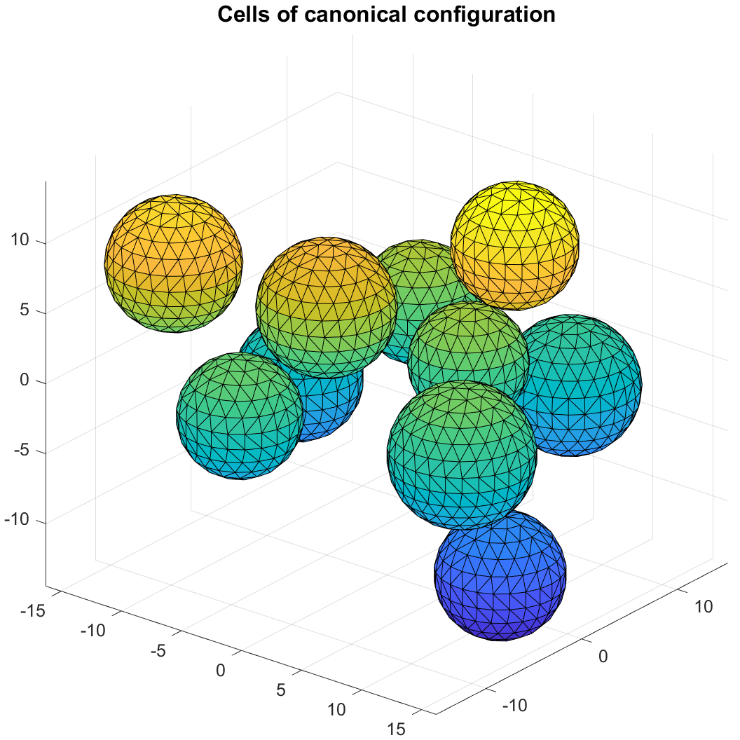
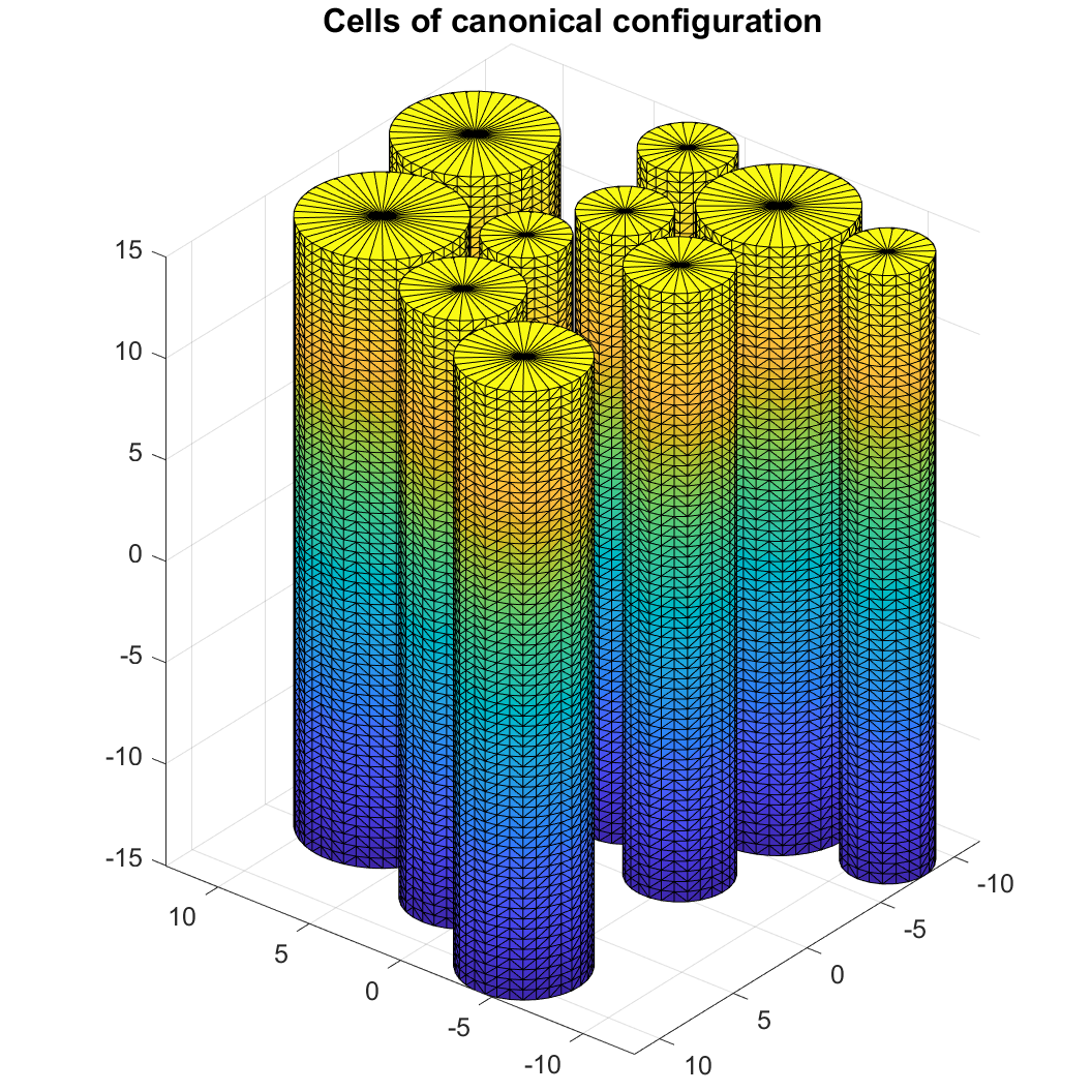
Figure 2: SpinDoctor plots cells in the canonical configuration.

3.4 Read simulation domain parameters

The user provides an input file for the simulation domain parameters, in the format described in Table 3.

Line	Variable name	Example	Explanation
1	Rratio	0.0	if Rratio is outside [0,1], it is set to 0; else $Rratio=\frac{R_{in}}{R_{out}}$;
2	include_ECS	2	0 = no ECS; 1 = box ECS; 2 = tight wrap ECS;
3	ECS_gap	0.3	ECS thickness: a. if box: as percentage of domain length; b. if tight wrap: as percentage of mean radius
4	dcoeff_IN	0.002	diffusion coefficient in IN cmpt: a. nucleus; b. axon (if there is myelin);
5	dcoeff_OUT	0.002	diffusion coefficient in OUT cmpt: a. cytoplasm; b. axon (if there is no myelin);
6	dcoeff_ECS	0.002	diffusion coefficient in ECS cmpt;
7	ic_IN	1	initial spin density in In cmpt: a. nucleus; b. axon (if there is myelin)
8	ic_OUT	1	initial spin density in OUT cmpt: a. cytoplasm; b. axon (if there is no myelin);
9	ic_ECS	1	initial spin density in ECS cmpt:
10	kappa_IN_OUT	1e-5	permeability between IN and OUT cmpts: a. between nucleus and cytoplasm; b. between axon and myelin;
11	kappa_OUT_ECS	1e-5	permeability between OUT and ECS cmpts: a. if no nucleus: between cytoplasm and ECS; b. if no myelin: between axon and ECS;
12	Htetgen	-1	Requested tetgen mesh size; -1 = Use tetgen default;
13	tetgen_cmd	’SRC/TETGEN/tetGen/win64/tetgen’	path to tetgen_cmd

Table 3: Input file of simulation domain parameters.

3.5 Create surface triangulation

Finite element mesh generation software requires a good surface triangulation. This means the surface triangulation needs to be water-tight and does not self-intersect. How closely these requirements are met in floating point arithmetic has a direct impact on the quality of the finite element mesh generated.

It is often difficult to produce a good surface triangulation for arbitrary geometries. Thus, we restrict the allowed shapes to cylinders and spheres. Below in Algorithms 2 and 3 we describe how to obtain a surface triangulation for spherical cells with nucleus, cylindrical cells with myelin layer, and the ECS (box or tightly wrapped). We describe a canonical configuration where the cylinders are placed parallel to the $z$-axis. More general shapes are obtained from the canonical configuration by coordinate transformation in a later step.

Suppose we have $n_{cell}$ spherical cells with nucleus. Denote a sphere with center $c$ and radius $R$ by $S(c,R)$, we use the built-in functions (convex hull, delaunnay triangulation) in MATLAB to get its surface triangulation, $T(c,R)$. Call the radii of the nucleus $r_{1},\cdots,r_{ncell}$ and the radii of the cells $R_{1},\cdots,R_{ncell}$. Then the boundaries between the cytoplasm and the nucleus are

$$\{\Gamma_{i}=T(c_{i},r_{i})\},i=1,\cdots,ncell;$$

and between the cytoplasm and the ECS

$$\{\Sigma_{i}=T(c_{i},R_{i})\},i=1,\cdots,ncell;$$

For the box ECS, we find the coordinate limits of the set

$$\bigcup_{i}S(c_{i},R_{i})\in[x_{0},x_{f}]\times[y_{0},y_{f}]\times[z_{0},z_{f}]$$

and add a gap $k=\text{ECS\_gap}\times\max\{x_{f}-x_{0},y_{f}-y_{0},z_{f}-z_{0}\}$ to make a box

$$B=[x_{0}-k,x_{f}+k]\times[y_{0}-k,y_{f}+k]\times[z_{0}-k,z_{f}+k].$$

We put 2 triangles on each face of $B$ to make a surface triangulation $\Psi$ with 12 triangles.

For the tight-wrap ECS, we increase the cell radius by a gap size and take the union

$$W=\bigcup_{i}S(c_{i},R_{i}+\text{ECS\_gap}\times R_{mean}),$$

where $R_{mean}=\frac{Rmin+Rmax}{2}$. We use the alphaShape function in MATLAB to find a surface triangulation $\Psi$ that contains $W$.

Algorithm 2 Surface triangulation of spherical cells and ECS.

Suppose we have $n_{cell}$ cylindrical cells with a myelin layer, all with height $H$. Denote a disk with center $c$ and radius $R$ by $D(c,R)$, and the circle with the same center and radius by $C(c,R)$. Let the radii of the axons be $r_{1},\cdots,r_{ncell}$ and the radii of the cells be $R_{1},\cdots,R_{ncell}$, meaning the thickness of the myelin layer is $R_{i}-r_{i}$.

The boundary between the axon and the myelin layer is:

$$C(c_{i},r_{i})\times[-H/2,H/2]$$

We discretize $C(c_{i},r_{i})$ as a polygon $P(c_{i},r_{i})$ and place one at $z=-H/2$ and one at $z=H/2$. Then we connect the corresponding vertices of $P(c_{i},r_{i})\times\{-H/2\}$ and $P(c_{i},r_{i})\times\{H/2\}$ and add a diagonal on each panel to get a surface triangulation $\Gamma_{i}$.

Between the myelin layer and the ECS we discretize $C(c_{i},R_{i})$ as a polygon and place one at $z=-H/2$ and one at $z=H/2$ to get a surface triangulation $\Sigma_{i}$.

For the box ECS, we find the coordinate limits of the union of $D(c_{i},R_{i})$ and add a gap to make a rectangle in two dimensions. Then we place the rectangle at $z=-H/2$ and at $z=H/2$ to get a box. Finally, the box is given a surface triangulation with 12 triangles.

For tight-wrap ECS, we increase the cell radius by a gap size and take the union

$$W=\bigcup_{i}D(c_{i},R_{i}+kR_{mean}).$$

We use the alphaShape function in MATLAB to find a two dimensional polygon $Q$ that contains $W$. We place $Q$ at $z=-H/2$ and at $z=H/2$ and connect correponding vertices, adding a diagonal on each panel. Suppose $Q$ is a polygon with $n$ vertices, then the surface triangulation of the side of the ECS will have $2n$ triangles.

The above procedure produces a surface triangulation for the boundaries that are parallel to $z$-axis. We now must close the top and bottom. The top and bottom boundaries is just the interior of $Q$. However, the surface triangulation cannot be done on $Q$ directly. We must cut out $D(c_{i},r_{i})$, the disk which touches the axon, and $A_{i}=D(c_{i},R_{i})-D(c_{i},r_{i})$, the annulus which touches the myelin. Then we triangulate $Q-\bigcup_{i}D_{i}-\bigcup_{i}A_{i}$ using the MATLAB built-in function that triangulates a polygon with holes to get the boundary that touches the ECS. The surface triangulation for $A_{i}$ and $D(c_{i},r_{i})$ are straightforward.

Algorithm 3 Surface triangulation of cylindrical cells and ECS.

3.6 Plot surface triangulation

SpinDoctor provides a routine to plot the surface triangulation (see Fig. 3).

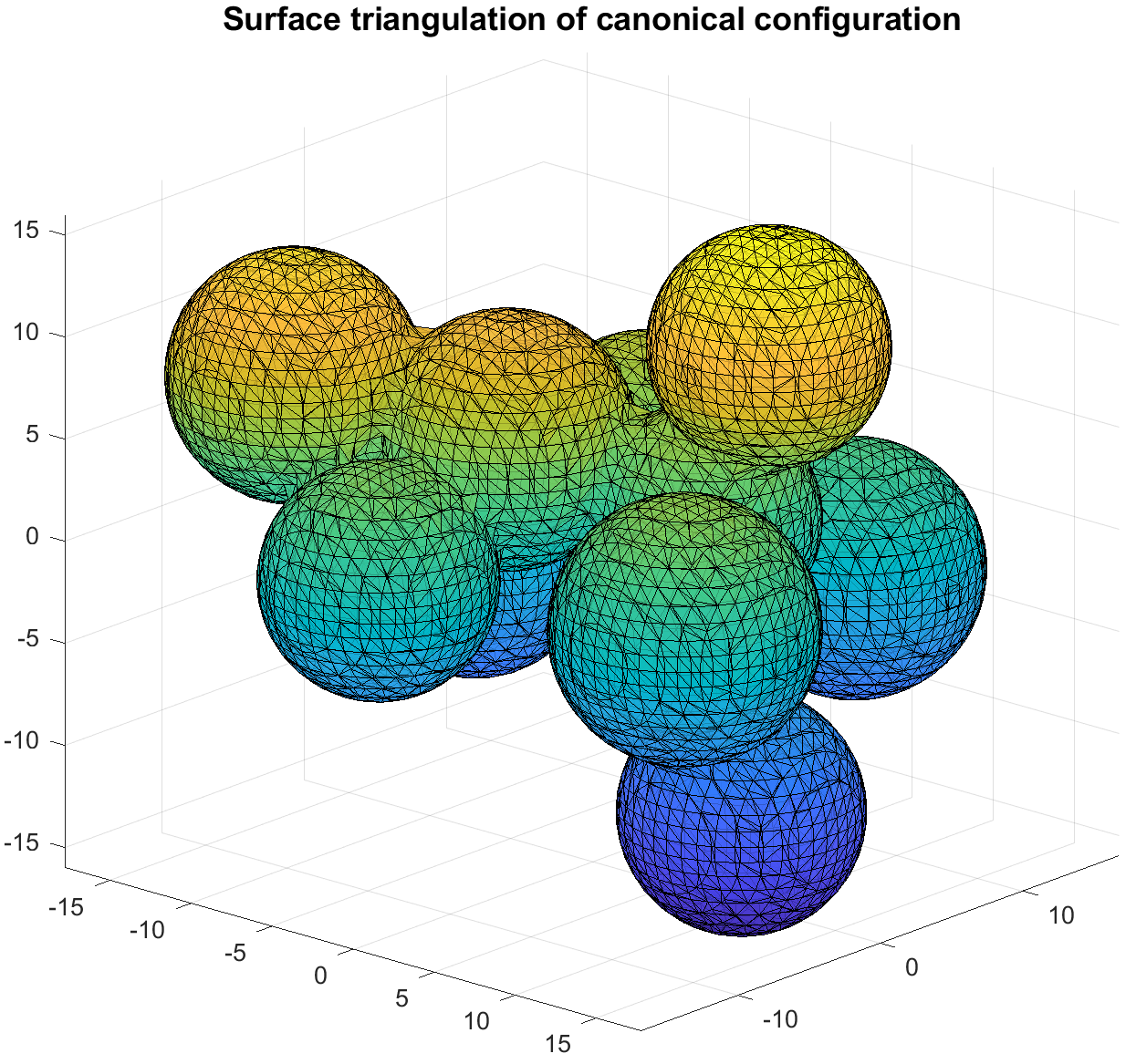
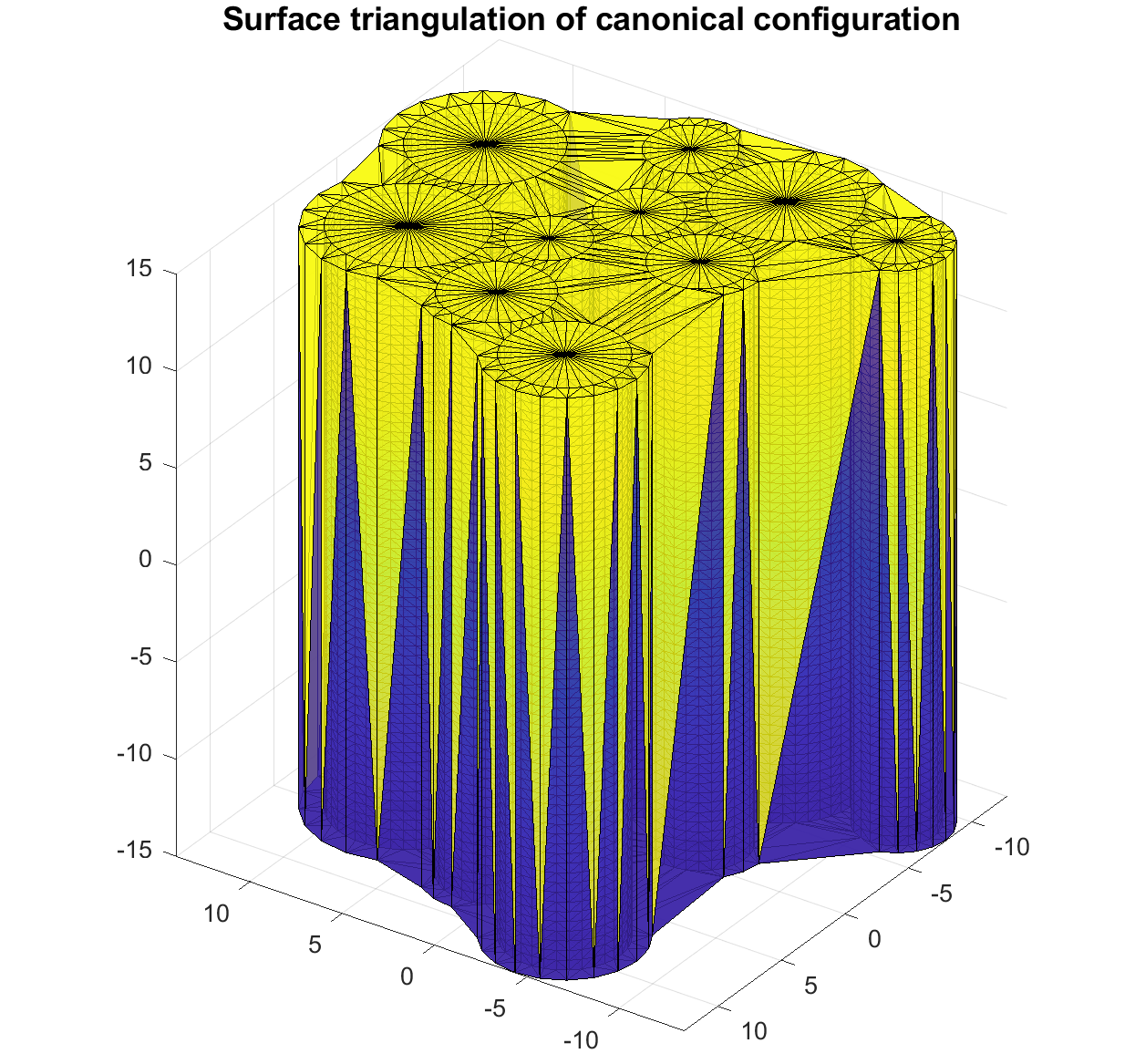
Figure 3: SpinDoctor plots the surface triangulation of the canonical configuration. Left: spherical cells with ECS; Right: cylindrical cells with ECS.

3.7 Finite element mesh generation

SpinDoctor calls Tetgen [42], an external package (executable files are included in the toolbox package), to create a tetrehedra finite elements mesh from the surface triangulation generated by Algorithms 2 and 3. The FE mesh is generated on the canonical configuration. The numbering of the compartments and boundaries used by SpinDoctor are given in Tables 4 and 5. The labels are related to the values of the intrinsic diffusion coefficient, the initial spin density, and the permeability requested by the user. Then the FE mesh nodes are deformed analytically by a coordinate transformation, described in Algorithm 4.

Spherical cells without nucleus
Cmpt	Cytoplasm	Nucleus	ECS
Label	OUT		ECS
Number	$[1:n_{cell}]$		$n_{cell}+1$
Spherical cells with nucleus
Cmpt	Cytoplasm	Nucleus	ECS
Label	OUT	IN	ECS
Number	$[1:n_{cell}]$	$[n_{cell}+1:2n_{cell}]$	$2n_{cell}+1$
Cylindrical cells without myelin
Cmpt	Axon	Myelin	ECS
Label	OUT		ECS
Number	$[1:n_{cell}]$		$n_{cell}+1$
Cylindrical cells with myelin
Cmpt	Axon	Myelin	ECS
Label	IN	OUT	ECS
Number	$[1:n_{cell}]$	$[n_{cell}+1:2n_{cell}]$	$2n_{cell}+1$

Table 4: The labels and numbers of compartments.

Spherical cells without nucleus
Boundary	Sphere		Outer ECS boundary
Label	OUT_ECS		$\kappa=0$
Number	$1:n_{cell}$		$n_{cell}+1$
Spherical cells with nucleus
Boundary	Outer sphere	Inner sphere	Outer ECS boundary
Label	OUT_ECS	IN_OUT	$\kappa=0$
Number	$1:n_{cell}$	$n_{cell}+1:2n_{cell}$	$2n_{cell}+1$
Cylindrical cells without myelin
Boundary	Cylinder side wall	Cylinder top and bottom	Outer ECS boundary minus cylinder top/bottom
Label	OUT_ECS	$\kappa=0$	$\kappa=0$
Number	$2[1:n_{cell}]-1$	$2[1:n_{cell}]$	$2n_{cell}+1$
Cylindrical cells with myelin
Boundary	Inner cylinder side wall	Inner cylinder top and bottom
Label	IN_OUT	$\kappa=0$
Number	$4[1:n_{cell}]-3$	$4[1:n_{cell}]-2$
	Outer cylinder side wall	Outer cylinder top and bottom	Outer ECS boundary minus cylinder top/bottom
Label	OUT_ECS	$\kappa=0$	$\kappa=0$
Number	$4[1:n_{cell}]-1$	$4[1:n_{cell}]$	$4n_{cell}+1$

Table 5: The labels and numbers of boundaries.

The external package Tetgen [42] generates the finite element mesh that keeps track of the different compartments and the interfaces between them. The mesh is saved in several text files.

The connectivity matrices of the finite elements and facets are not modified by the coordinates transformation described below. The nodes are transformed by bending and twisting as described next.

The set of FE mesh nodes $\{x_{i},y_{i},z_{i}\}$ are transformed in the following ways:

Twisting around the $z$-axis with a user-chosen twisting parameter $\alpha_{twist}$ is defined by

$$\begin{split}\begin{bmatrix}x\\ y\\ z\end{bmatrix}&\rightarrow\begin{bmatrix}\cos(\alpha_{twist}z)&-\sin(\alpha_{twist}z)&0\\ \sin(\alpha_{twist}z)&\cos(\alpha_{twist}z)&0\\ 0&0&1\end{bmatrix}\begin{bmatrix}x\\ y\\ z\end{bmatrix}.\end{split}$$

Bending on the $x-z$ plane with a user-chosen bending parameter $\alpha_{bend}$ is defined by

$$\begin{bmatrix}x\\ y\\ z\end{bmatrix}\rightarrow\begin{bmatrix}x+\alpha_{bend}z^{2}\\ y\\ z\end{bmatrix}.$$

Given $[\alpha_{bend},\alpha_{twist}]$, bending is performed after twisting.

Algorithm 4 Bending and twisting of the FE mesh of the canonical configuration.

3.8 Plot FE mesh

SpinDoctor provides a routine to plot the FE mesh (see Fig. 4 for cylinders and ECS that have been bent and twisted).

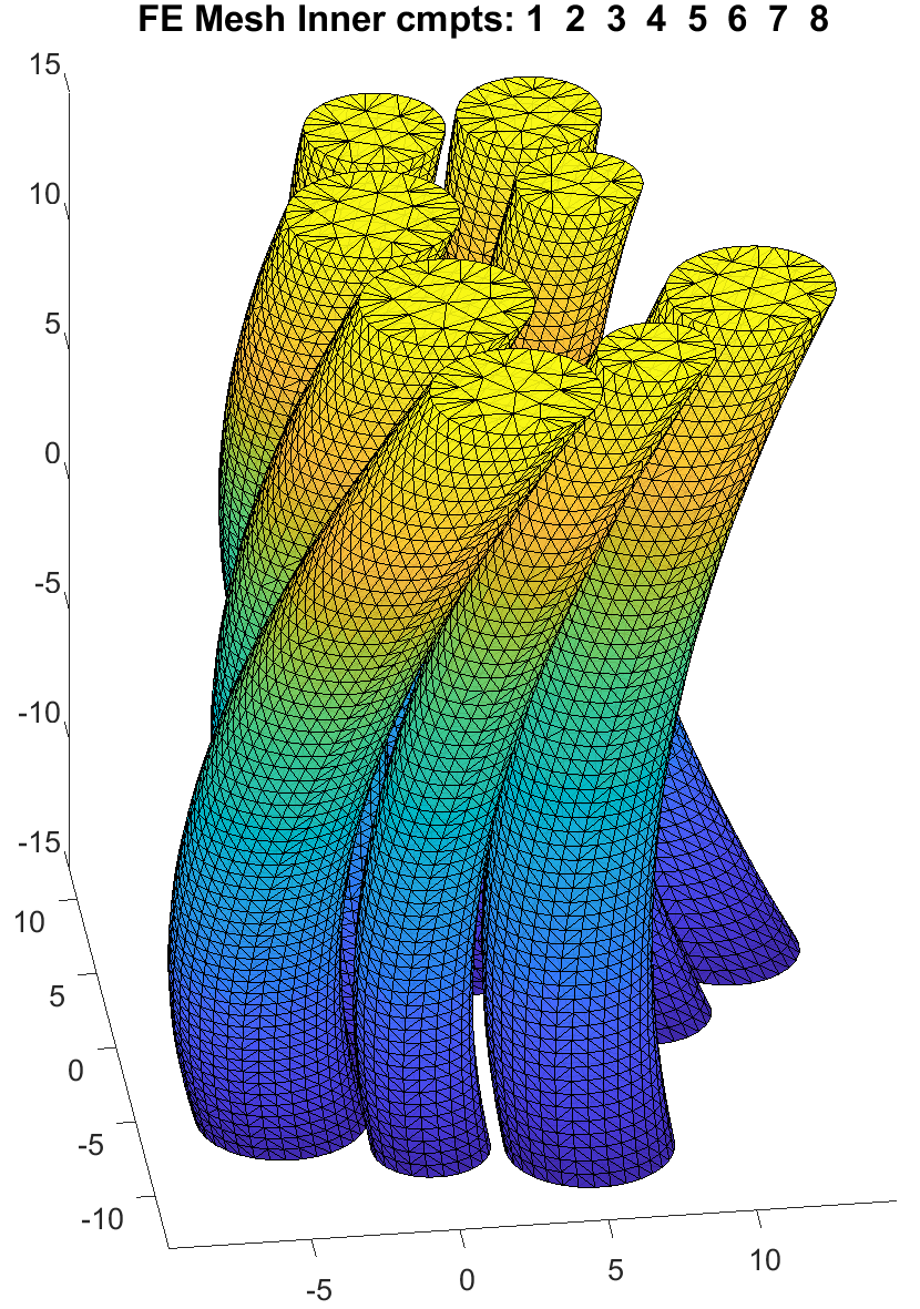
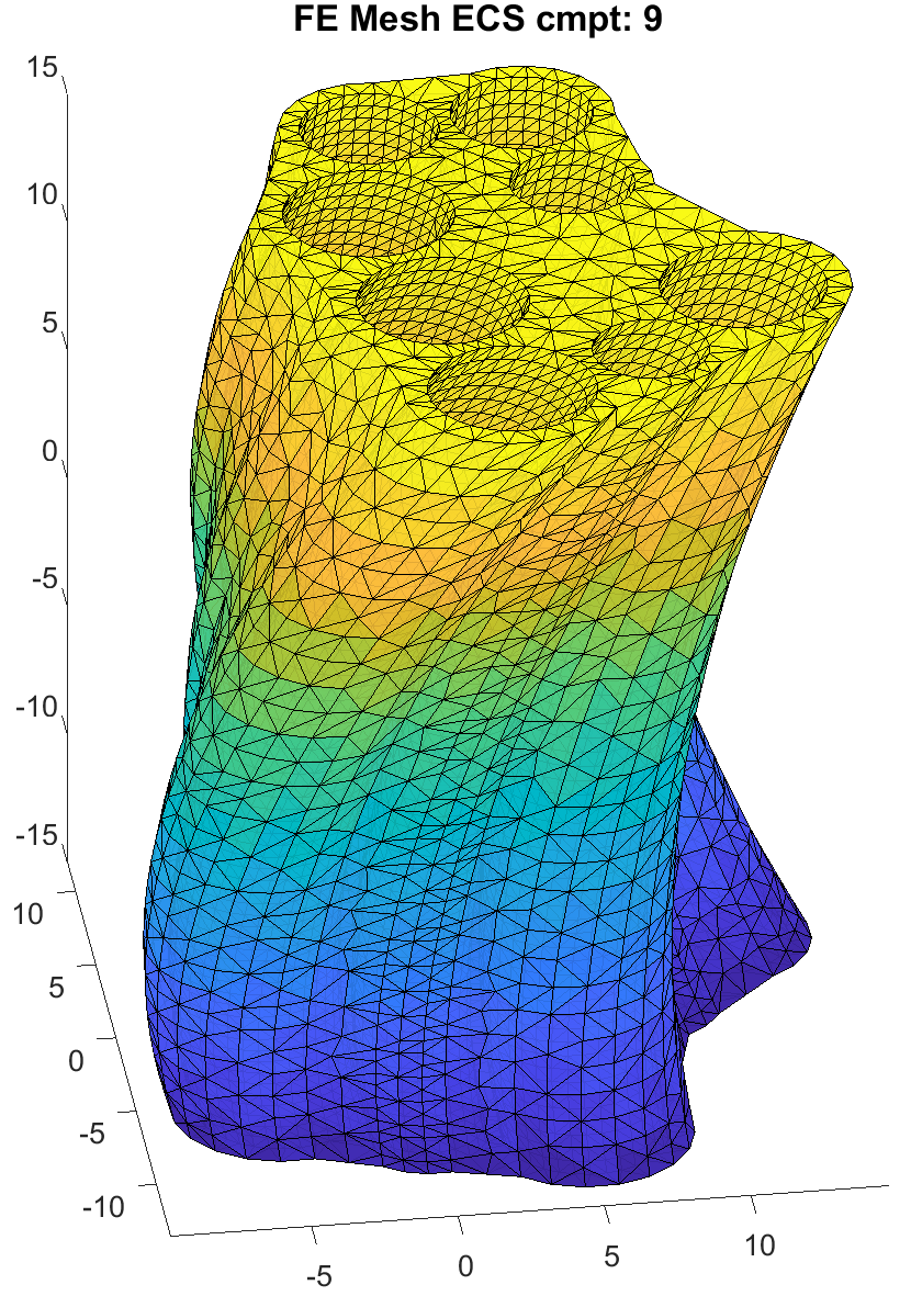
Figure 4: FE mesh of cylinders and ECS after bending and twisting. Compartment number is 1 to 8 for the cylinders and 9 for the ECS.

3.9 Read experimental parameters

The user provides an input file for the simulation experimental parameters, in the format described in Table 6.

Line	Variable name	Example	Explanation
1	ngdir	20	number of gradient direction; if $ngdir>1$, the gradient directions are distributed uniformly on a sphere; if $ngdir=1$, take the gradient direction from the line below;
2	gdir	1.0 0.0 0.0	gradient direction; No need to normalize;
3	nexperi	3	number of experiments;
4	sdeltavec	2500 10000 10000	small delta;
5	bdeltavec	2500 10000 10000	big delta;
6	seqvec	1 2 3	diffusion sequence of experiment; 1 = PGSE; 2 = OGSEsin; 3 = OGSEcos;
7	npervec	0 10 10	number of period of OGSE;
8	solve_hadc	1	0 = do not solve HADC; Otherwise solve HADC;
9	rtol_deff, atol_deff	1e-4 1e-4	$[r_{tol}\quad a_{tol}]$; relative and absolute tolerance for HADC ODE solver;
10	solve_btpde	1	0 = do not solve BTPDE; Otherwise solve BTPDE;
11	rtol_bt, atol_bt	1e-5 1e-5	$[r_{tol}\quad a_{tol}]$; relative and absolute tolerance for BTPDE ODE solver;
12	nb	2	number of b-values;
13	blimit	0	0 = specify bvec; 1 = specify [bmin,bmax]; 2 = specify [gmin,gmax];
14	const_q	0	0: use input bvalues for all experiments; 1: take input bvalues for the first experiment and use the same q for the remaining experiments
15	bvalues	0 50 100 200	bvalues or [bmin, bmax] or [gmin, gmax]; depending on line 13;

Table 6: Input file for simulation experiment parameters.

3.10 BTPDE

The spatial discretization of the BTPDE is based on a finite element method where interface (ghost) elements [35] are used to impose the permeable interface conditions. The time stepping is done using the MATLAB built-in ODE routine ode23t. See Algorithm 5.

FE matrices are generated for each compartment by the finite element method with continuous piecewise linear basis functions (known as $P_{1}$). The basis functions are denoted as $\varphi_{k}$ for $k=1,\dots,N_{v}$, where $N_{v}$ denotes the number of mesh nodes (vertices). All matrices are sparse matrices. $\bm{M}$ and $\bm{S}$ are known in the FEM literature as mass and stiffness matrices which are defined as follows:

$$\bm{M}_{ij}=\int_{\Omega}\varphi_{i}\varphi_{j}\,d{\bm{x}},\qquad\qquad\bm{S}_{ij}=\int_{\Omega}\sigma_{i}\,\nabla\varphi_{i}\cdot\nabla\varphi_{j}\,d{\bm{x}}.$$

$\bm{J}$ has a similar form as the mass matrix but it is scaled with the coefficient ${\bm{g}}\cdot{\bm{x}}$, we therefore call it the scaled-mass matrix

$$\bm{J}_{ij}=\int_{\Omega}{\bm{g}}\cdot{\bm{x}}\,\varphi_{i}\varphi_{j}\,d{\bm{x}}.$$

We construct the matrix based on the flux matrix $\bm{Q}$

$$\bm{Q}_{ij}=\int_{\partial\Omega}w\,\varphi_{i}\varphi_{j}\,ds$$

where a scalar function $w$ is used as an interface marker. The matrices are assembled from local element matrices and the assembly process is based on vectorized routines of [43], which replace expensive loops over elements by operations with 3-dimensional arrays. All local elements matrices in the assembly of $\bm{S},\bm{M},\bm{J}$ are evaluated at once and stored in a full matrix of size $4\times 4\times N_{e}$, where $N_{e}$ denotes the number of tetrahedral elements. The assembly of $\bm{Q}$ is even simpler; all local matrices are stored in a full matrix of size $3\times 3\times n_{be}$, where $n_{be}$ denotes the number of boundary triangles.

Double nodes are placed at the interfaces between compartments connected by permeable membrane. $\overline{\bm{Q}}$ is used to impose the interface conditions and it is associated with the interface (ghost) elements. Specifically, assume that the double nodes are defined in a pair of indices $\{i,\bar{i}\}$, $\overline{\bm{Q}}$ is defined as the following

$$\overline{\bm{Q}}_{ij}=\begin{cases}\bm{Q}_{ij},&\mbox{if vertex $i$ and $j$ belong to one interface}\\ -\bm{Q}_{\bar{i}\bar{j}}&\mbox{if vertex $i$ and $j$ belong to two different interfaces}\end{cases}$$

The fully coupled linear system has the following form

$$\bm{M}\frac{\partial\xi}{\partial t}=-\Bigl{(}I\gamma f(t)\,{\bm{J}}+\bm{S}+\overline{\bm{Q}}\Bigl{)}\,\xi$$ (14)

where $\xi$ is the approximation of the magnetization $M$. SpinDoctor calls MATLAB built-in ODE routine ode23t to solve the semi-discretized system of equations.

Algorithm 5 BTPDE.

3.11 HADC model

Similarly, the DE of the HADC model is discretized by finite elements. See Algorithm 6.

Eq. (12) can be discretized similarly as described for the BTPDE and has the matrix form

$$\bm{M}\frac{\partial\zeta}{\partial t}=-\bm{S}\,\zeta+{\bm{Q}}\,\bar{\zeta}$$ (15)

where $\zeta$ is the approximation of $w$ and $\bar{\zeta}_{i}=\sigma_{i}\,F(t)\,{\bm{u}}_{g}\cdot{\bm{n}}({\bm{x}}_{i})$. We note that the matrices here are assembled and solved separately for each compartment. SpinDoctor calls MATLAB built-in ODE routine ode23t to solve the semi-discretized equation.

Algorithm 6 HADC model.

3.12 Some important output quantities

In Table 7 we list some useful quantities that are the outputs of SpinDoctor. The braces in the ”Size” column denote MATLAB cell data structure and the brackets denote MATLAB matrix data structure.

Variable name	Size	Explanation
TOUT	{nexperi$\times$nb$\times$Ncmpt}[1 $\times$nt]	ODE time discretization
YOUT	{nexperi$\times$nb$\times$Ncmpt}[Nnodes $\times$nt]	Magnetization
MF_cmpts	[Ncmpt $\times$ nexperi $\times$ nb]	integral of magnetization at $TE$ in each compartment.
MF_allcmpts	[nexperi $\times$ nb]	integral of magnetization at $TE$ summed over all compartments.
ADC_cmpts	[Ncmpt $\times$ nexperi ]	ADC in each compartment.
ADC_allcmpts	[nexperi $\times$ 1]	ADC accounting for all compartments.
ADC_cmpts_dir	[ngdir $\times$ Ncmpt $\times$ nexperi ]	ADC in each compartment in each direction.
ADC_allcmpts_dir	[ngdir $\times$ nexperi $\times$ 1]	ADC accounting for all compartments in each direction.

Table 7: Some important SpinDoctor output quantities.

4 SpinDoctor examples

In this section we show some prototypical examples using the available functionalities of SpinDoctor.

4.1 Comparison of BTPDE and HADC with Short Time Approximation

In Fig. 5 we show that both BTPDE and HADC solutions match the STA values at short diffusion times for cylindrical cells (compartments 1 to 5). We also show that for the ECS (compartment 6), the STA is too low, because it does not account for the fact that spins in the ECS can diffuse around several cylinders. This also shows that when the interfaces are impermeable, the BTPDE ADC and that from the HADC model are identical. The diffusion-encoding sequence here is cosine OGSE with 6 periods.

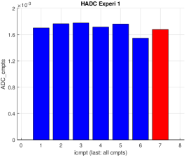
Figure 5: Geometry: 5 cylinders, tight wrap ECS, ECS gap = 0.2, ${\bm{u_{g}}}=[1,1,1]$, $\sigma^{out}=\sigma^{ecs}=2\times 10^{-3}\,\text{mm}^{2}/\text{s}$, $\kappa=0\,\text{m}/\text{s}$, OGSE cosine ($\delta=14\text{ms},\Delta=14\text{ms}$, number of periods = 6). The vertical bars indicate the ADC in each compartment. The ADC in the rightmost position is the ADC that takes into account the diffusion in all the compartments.

4.2 Permeable membranes

In Fig. 6 we show the effect of permeability: the BTPDE model includes permeable membranes ($\kappa=1\times 10^{-3}\,\text{m}/\text{s}$) whereas the HADC has impermeable membranes. We see in the permeable case, the ADC in the spheres are higher than in the impermeable case, whereas the ECS show reduced ADC because the faster diffusing spins in the ECS are allowed to moved into the slowly diffusing spherical cells. We note that in the permeable case, the ADC in each compartment is obtained by using the fitting formula involving the logarithm of the dMRI signal, and we defined the ”signal” in a compartment as the total magnetization in that compartment at TE, which is just the integral of the solution of the BTPDE in that compartment.

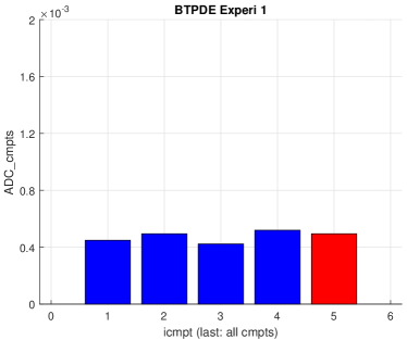
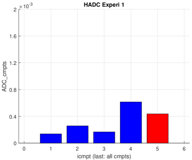
Figure 6: Geometry: 3 spheres, tight wrap ECS, ECS gap = 0.3, ${\bm{u_{g}}}=[1,1,0]$, $\sigma^{in}=\sigma^{ecs}=2\times 10^{-3}\,\text{mm}^{2}/\text{s}$, $\kappa=1\times 10^{-3}\,\text{m}/\text{s}$ (left), $\kappa=0\,\text{m}/\text{s}$ (right). PGSE ($\delta=5\text{ms},\Delta=5\text{ms}$). The vertical bars indicate the ADC in each compartment. The ADC in the rightmost position is the ADC that takes into account the diffusion in all the compartments.

4.3 Myelin layer

In Fig. 7 we show the diffusion in cylindrical cells, the myelin layer, and the ECS. The ADC is higher in the myelin layer than in the cells, because for spins in the myelin layer diffusion occurs in the tangential direction (around the circle). At longer diffusion times, the ADC of both the myelin layer and the cells becomes very low. The ADC is the highest in the ECS, because the diffusion distance can be longer than the diameter of a cell, since the diffusing spins can move around multiple cells.

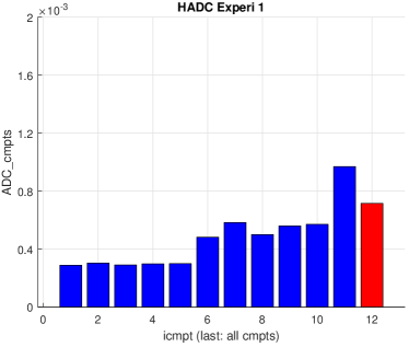
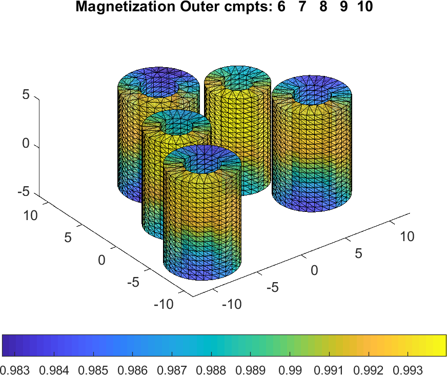
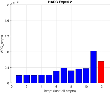
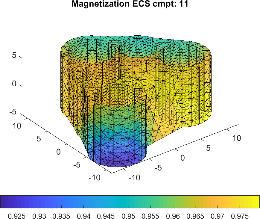
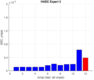
Figure 7: Geometry: 5 cylinders, myelin layer, $R_{in}/R_{out}=0.5$, tight wrap ECS, ECS gap = 0.3, $\kappa=0\,\text{m}/\text{s}$, ${\bm{u_{g}}}=[1,1,1]$, $\sigma^{in}=\sigma^{out}=\sigma^{ecs}=2\times 10^{-3}\,\text{mm}^{2}/\text{s}$, 3 experiments: PGSE ($\delta=5\text{ms},\Delta=5,10,20\text{ms}$). Left: the magnetization at $\Delta=5\text{ms}$. Right: the ADC values. The vertical bars indicate the ADC in each compartment. The ADC in the rightmost position is the ADC that takes into account the diffusion in all the compartments.

4.4 Twisting and bending

In Fig. 8 we show the effect of bending and twising in cylindrical cells in multiple gradient directions. The HADC is obtained in 20 directions uniformly distributed in the sphere. We used spherical harmonics interpolation to interpolate the HADC in the entire sphere. Then we deformed the radius of the unit sphere to be proportional to the interpolated HADC and plotted the 3D shape. The color axis also indicates the value of the interpolated HADC.

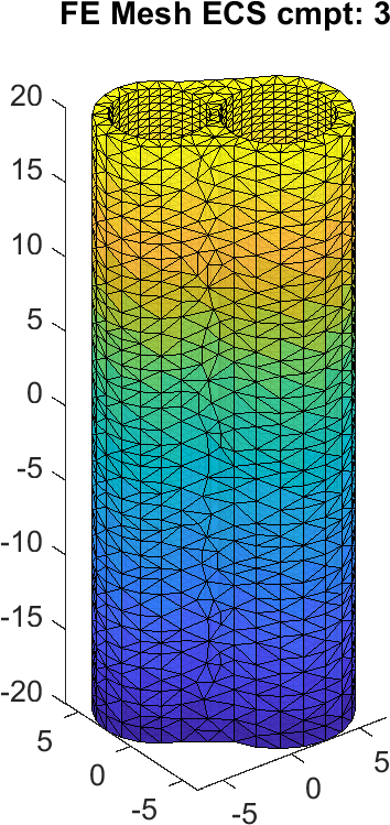
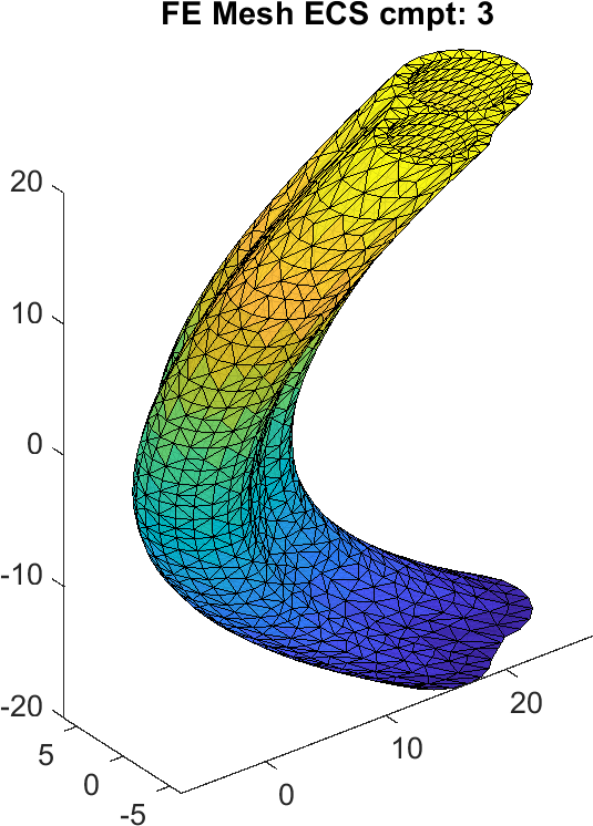
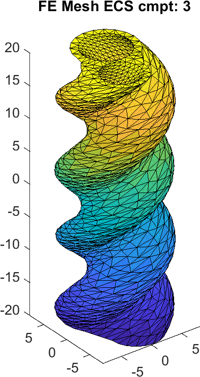
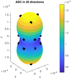
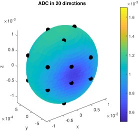
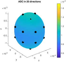
Figure 8: Geometry: 2 cylinders, no myelin layer, tight wrap ECS, ECS gap = 0.3, $\kappa=0\,\text{m}/\text{s}$, $\sigma^{out}=\sigma^{ecs}=2\times 10^{-3}\,\text{mm}^{2}/\text{s}$, PGSE ($\delta=2.5\text{ms},\Delta=5\text{ms}$).
Left: canonical configuration. Middle: bend parameter = 0.05. Right: twist parameter = 0.30. Top: FE mesh of the ECS (the FE mesh of the axon compartments numbered 1 and 2 not shown). Bottom: interpolated values of the HADC on the unit sphere, and then the sphere was distorted to reflect the value of the HADC. The color axis also gives the value of the HADC in the various gradient directions. The black dots indicate the 20 original gradient-directions in which the HADC was simulated. The spherical harmonics interpolation takes the 20 original directions into 900 directions uniformly distributed on the sphere.

4.5 Timing

In Table 8 we give the average computational times for solving the BTPDE and the HADC. All simulations were performed on a laptop computer with the processor Intel(R) Core(TM) i5-4210U CPU @ 1.70 GHz 2.40 GHz, running Windows 10 (1809). The geometrical configuration includes 2 axons and a tight wrap ECS, the simulated sequence is PGSE ($\delta=2.5\text{ms},\Delta=5\text{ms}$). In the impermeable case, the compartments are uncoupled, and the computational times are given separately for each compartment. In the permeable membrane case, the compartments are coupled, and the computational time is for the coupled system (relevant to the BTPDE only).

	FE mesh size	BTPDE	BTPDE	HADC
		$b=50\,\text{s/mm}^{2}$	$b=1000\,\text{s/mm}^{2}$
Uncoupled: Axons	5865 nodes, 19087 ele	7.89 sec	9.07 sec	8.80 sec
Uncoupled: ECS	6339 nodes, 19618 ele	10.14 sec	13.95 sec	11.87 sec
Coupled: Axons+ECS	7344 nodes, 38705 ele	39.14 sec	43.24 sec	N/A

Table 8: Computational times for solving the BTPDE and the HADC. All simulations were performed on Intel(R) Core(TM) i5-4210U CPU @ 1.70 GHz 2.40 GHz, running Windows 10 (1809). The geometrical configuration includes 2 axons and a tight wrap ECS, the simulated sequence is PGSE ($\delta=2.5\text{ms},\Delta=5\text{ms}$).

5 Numerical validation of SpinDoctor

In this section, we validate SpinDoctor by comparing SpinDoctor with the Matrix Formalism method [49, 50] in a simple geometry. The Matrix Formalism method is a closed form representation of the dMRI signal based on the eigenfunctions of the Laplace operator subject to homogeneous Neumann boundary conditions. These eigenfunctions are available in explicit form for elementary geometries such as the line segment, the disk, and the sphere [51, 52, 53, 54]. The dMRI signal obtained using the Matrix Formalism method will be considered the reference solution in this section.

The accuracy of the SpinDoctor simulations can be tuned using three simulation parameters:

1. $Htetgen$ controls the finite element mesh size;

   1. $Htetgen=-1$ means the FE mesh size is determined automatically by the internal algorithm of Tetgen to ensure a good quality mesh (subject to the constraint that the radius to edge ratio of tetrahedra is no larger than 2.0).

   2. $Htetgen=h$ requests a desired FE mesh tetrahedra height of $h$ $\mu\text{m}$ (in later versions of Tetgen, this parameter has been changed to the desired volume of the tetrahedra).

2. $rtol$ controls the accuracy of the ODE solve. It is the relative residual tolerance at all points of the FE mesh at each time step of the ODE solve;

3. $atol$ controls the accuracy of the ODE solve. It is the absolute residual tolerance at all points of the FE mesh at each time step of the ODE solve;

We varied the finite element mesh size and the ODE solve accuracy of SpinDoctor and ran 6 simulations with the following simulation parameters:

1. $rtol=10^{-3}$, $atol=10^{-6}$, $Htetgen=-1$;

2. $rtol=10^{-6}$, $atol=10^{-9}$, $Htetgen=-1$;

3. $rtol=10^{-9}$, $atol=10^{-12}$, $Htetgen=-1$;

4. $rtol=10^{-3}$, $atol=10^{-6}$, $Htetgen=1$;

5. $rtol=10^{-6}$, $atol=10^{-9}$, $Htetgen=1$;

6. $rtol=10^{-9}$, $atol=10^{-12}$, $Htetgen=1$;

   The geometry simulated is the following:

   • 3LayerCylinder is a 3-layer cylindrical geometry of height $1\mu\text{m}$ and the layer radii, $R_{1}=2.5\mu\text{m}$, $R_{2}=5\mu\text{m}$ and $R_{3}=10\mu\text{m}$. The middle layer is subject to permeable interface conditions on both the interior and the exterior interfaces, with permeability coefficient $\kappa$. The exterior boundary $R=R_{3}$ is subject to impermeable boundary conditions. The top and bottom boundaries are also subject to impermeable boundary conditions.

   • For this geometry, $Htetgen=-1$ gives finite elements mesh size ($n_{nodes}=440,n_{elem}=1397$). $Htetgen=1$ gives finite elements mesh size ($n_{nodes}=718,n_{elem}=2088$).

   The dMRI experimental parameters are the following:

   • the diffusion coefficient in all compartments is $2\times 10^{-3}\,\text{mm}^{2}/\text{s}$;

   • the diffusion-encoding sequence is PGSE ($\delta=10\text{ms}$, $\Delta=13\text{ms}$);

   • 8 b-values: $b=\{0,100,500,1000,2000,3000,6000,10000\}\,\text{s/mm}^{2}$;

   • 1 gradient direction: $[1,1,0]$;

   In Figure 9 we show the signal differences (in percent) of the reference Matrix Formalism method and the SpinDoctor simulations, normalized by the reference signal at $b=0$:

   $$E(b)=\frac{\left|S^{MF}(b)-S^{SpinD}(b)\right|}{S^{MF}(b=0)}\times 100.$$ (16)

   We see that the signal difference is less than $0.35\%$ for $\kappa=10^{-5}\,\text{m}/\text{s}$ and it is less than $0.25\%$ for $\kappa=10^{-4}\,\text{m}/\text{s}$ for all 6 SpinDoctor simulations. The signal difference becomes smaller when the ODE solve tolerances are changed from ($rtol=10^{-3}$, $atol=10^{-6}$) to ($rtol=10^{-6}$, $atol=10^{-9}$), but there is no change when the tolerances are further reduced to ($rtol=10^{-9}$, $atol=10^{-12}$). If we refine the FE mesh, but keep the ODE solve tolerances the same, the signal difference is in fact larger using the refined mesh than using the coarse mesh at the smaller b-values, though this effect disappears at higher b-values and larger permeability. This is probably due to parasitic oscillatory modes on the finer mesh that need smaller time steps to be sufficiently damped.

   

   

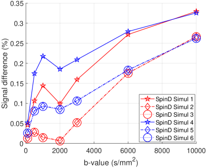
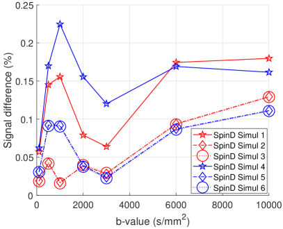
   Figure 9: Signal difference between the Matrix Formalism signal (reference) and the SpinDoctor signal. Left: $\kappa=10^{-5}\,\text{m}/\text{s}$. Right: $\kappa=10^{-4}\,\text{m}/\text{s}$. The geometry is 3LayerCylinder. The diffusion coefficient in all compartments is $2\times 10^{-3}\,\text{mm}^{2}/\text{s}$; the diffusion-encoding sequence is PGSE ($\delta=10\text{ms}$, $\Delta=13\text{ms}$); Simul 1: $rtol=10^{-3}$, $atol=10^{-6}$, $Htetgen=-1$; Simul 2: $rtol=10^{-6}$, $atol=10^{-9}$, $Htetgen=-1$; Simul 3: $rtol=10^{-9}$, $atol=10^{-12}$, $Htetgen=-1$; Simul 4: $rtol=10^{-3}$, $atol=10^{-6}$, $Htetgen=1$; Simul 5: $rtol=10^{-6}$, $atol=10^{-9}$, $Htetgen=1$; Simul 6: $rtol=10^{-9}$, $atol=10^{-12}$, $Htetgen=1$;

   6 Computational time and comparison with Monte-Carlo simulation

   In this section, we compare SpinDoctor with Monte-Carlo simulation using the publicly available software package Camino Diffusion MRI Toolkit [26], downloaded from http://cmic.cs.ucl.ac.uk/camino. All the simulations were performed on a server computer with 12 processors (Intel (R) Xeon (R) E5-2667 @2.90 GHz), 192 GB of RAM, running CentOS 7. SpinDoctor was run using MATLAB R2019a on the same computer.

   We give SpinDoctor computational times for three relatively complicated geometries. We also give Camino computational times for the first two geometries. We did not use Camino for the third geometry due to the excessive time required by Camino.

   The number of the degrees of freedom in the SpinDoctor simulations is the finite element mesh size (the number of nodes and the number of elements). For Camino it is the number of spins. The time stepping choice of the SpinDoctor simulations is given by the ODE solve tolerances. For Camino it is given by the number of time steps. Camino has an initialization step where it places the spins and we give the time of this initialization step separately from the Camino random walk simulation time.

   Given the interest of the dMRI community in the extra-cellular space [11] and neuron simulations, we chose the following three geometries:

   1. ECS400axons. See Figure 10. This models the extra-cellular space outside of 400 axons. We generated 400 cylinders with height $1\mu\text{m}$ and radii ranging from $2-5\mu\text{m}$, randomly placed according to Algorithm 1. The small height of the cylinders means that this geometry should be used only for studying transverse diffusion. We used a tight-wrap ECS: this choice means we do not need to have a complicated algorithm to avoid large empty spaces as would be the case when the ECS is box-shaped.

   2. DendriteBranch. See Figure 11. This is a dendrite branch whose original morphological reconstruction SWC file published in NeuroMorpho.Org [55]. By wrapping the geometry described in the SWC file in a new watertight surface and using the external FE meshing package GMSH [56], we created a FE mesh for this dendrite branch. The FE mesh was in imported and used in SpinDoctor. We note this is an externally generated FE mesh and this illustrate the capacity of SpinDoctor to simulate the dMRI on general geometries provided by the user.

   3. ECS200axons. See Figure 12. This models the extra-cellular space outside of 200 axons. To study 3-dimensional diffusion, the height of the cylinders was increased to $50\mu\text{m}$. To keep the finite element mesh size reasonable, we decreased the number of axons to 200, keeping the range of radii between $2-5$ microns, placed randomly as above, with a tight-wrap ECS.

   

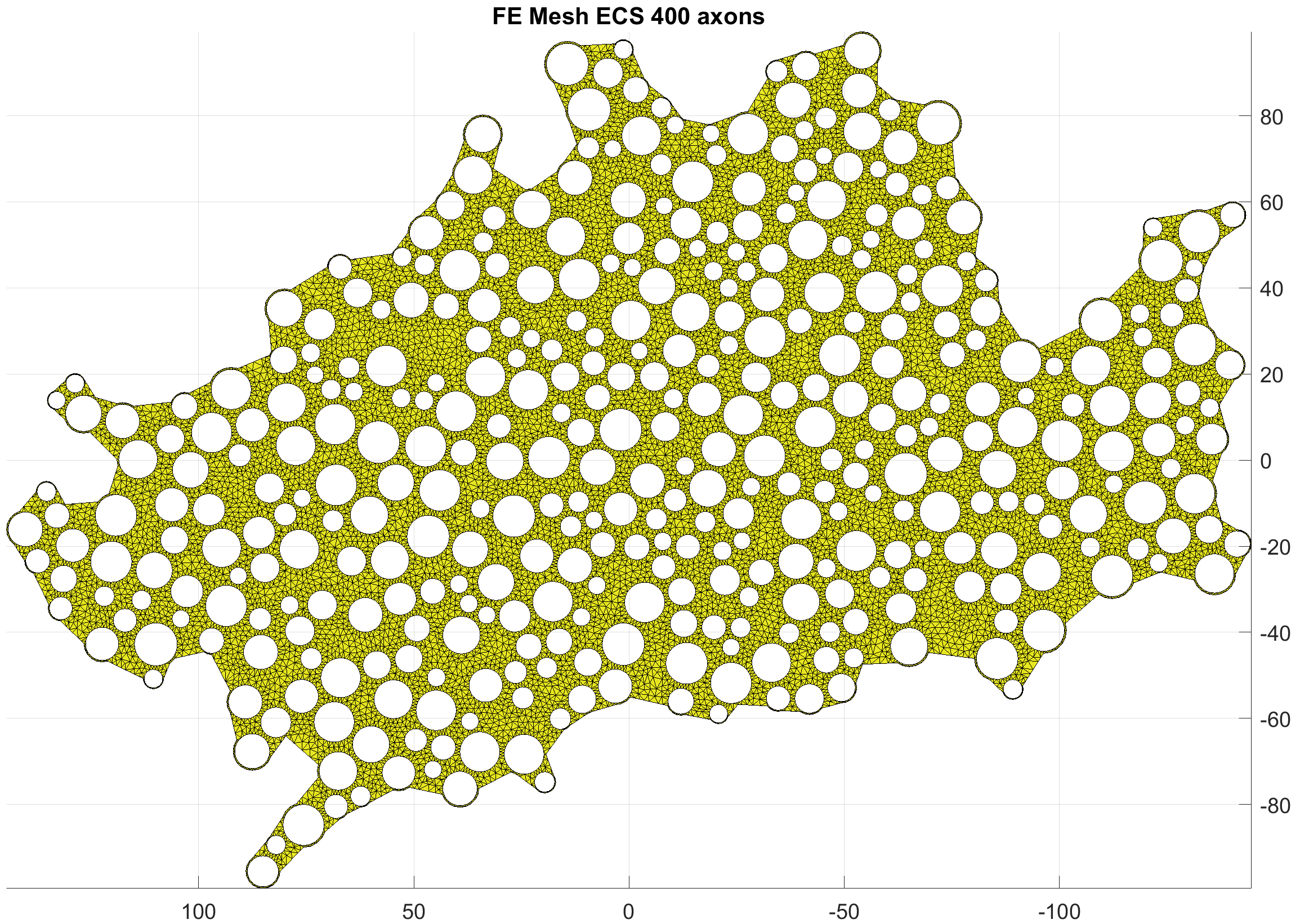
   Figure 10: The geometry is ECS400axons. This finite elements mesh size is ($n_{nodes}=53280,n_{elem}=125798$).

   

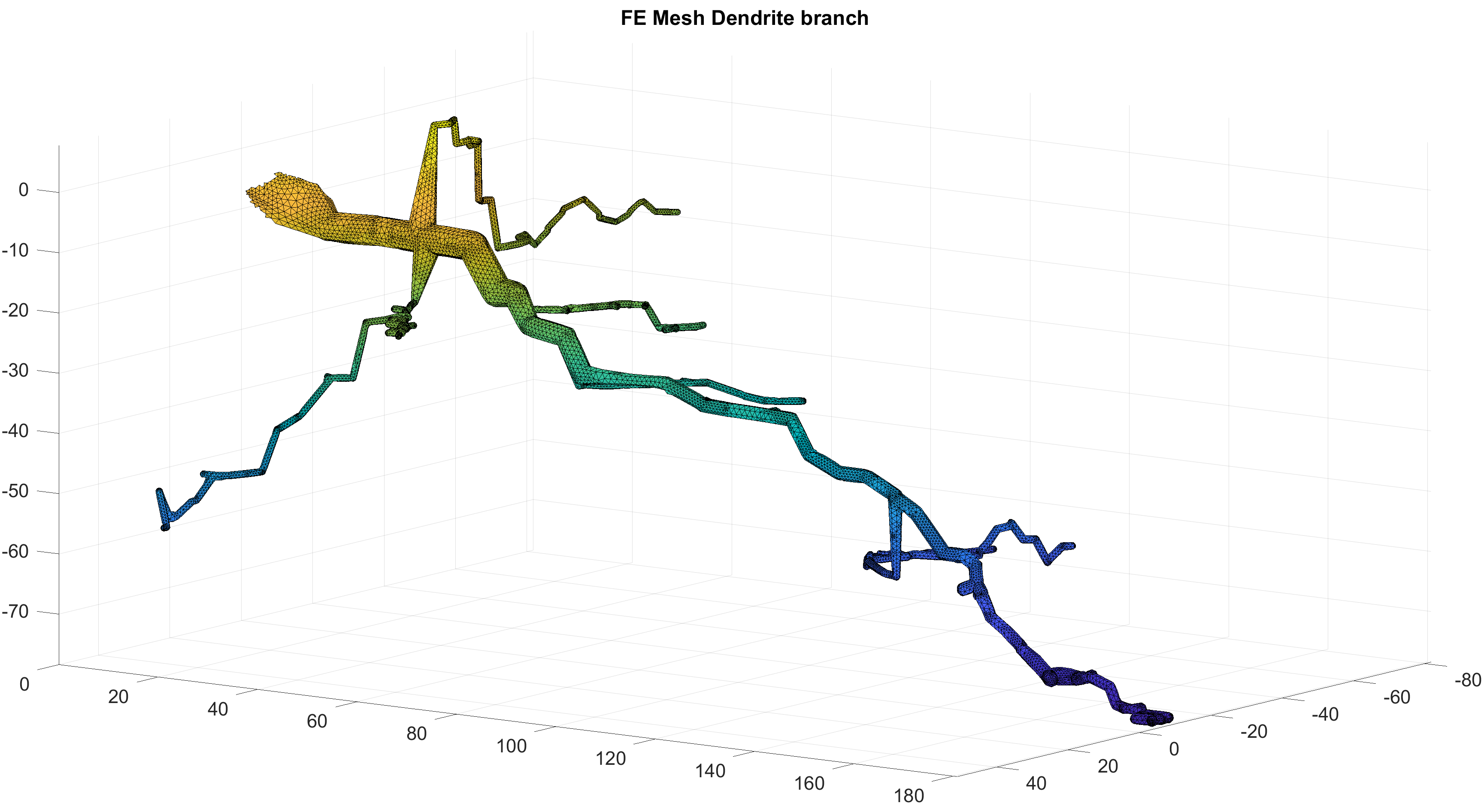
   Figure 11: The geometry is DendriteBranch. This finite elements mesh size is ($n_{nodes}=24651,n_{elem}=91689$)

   

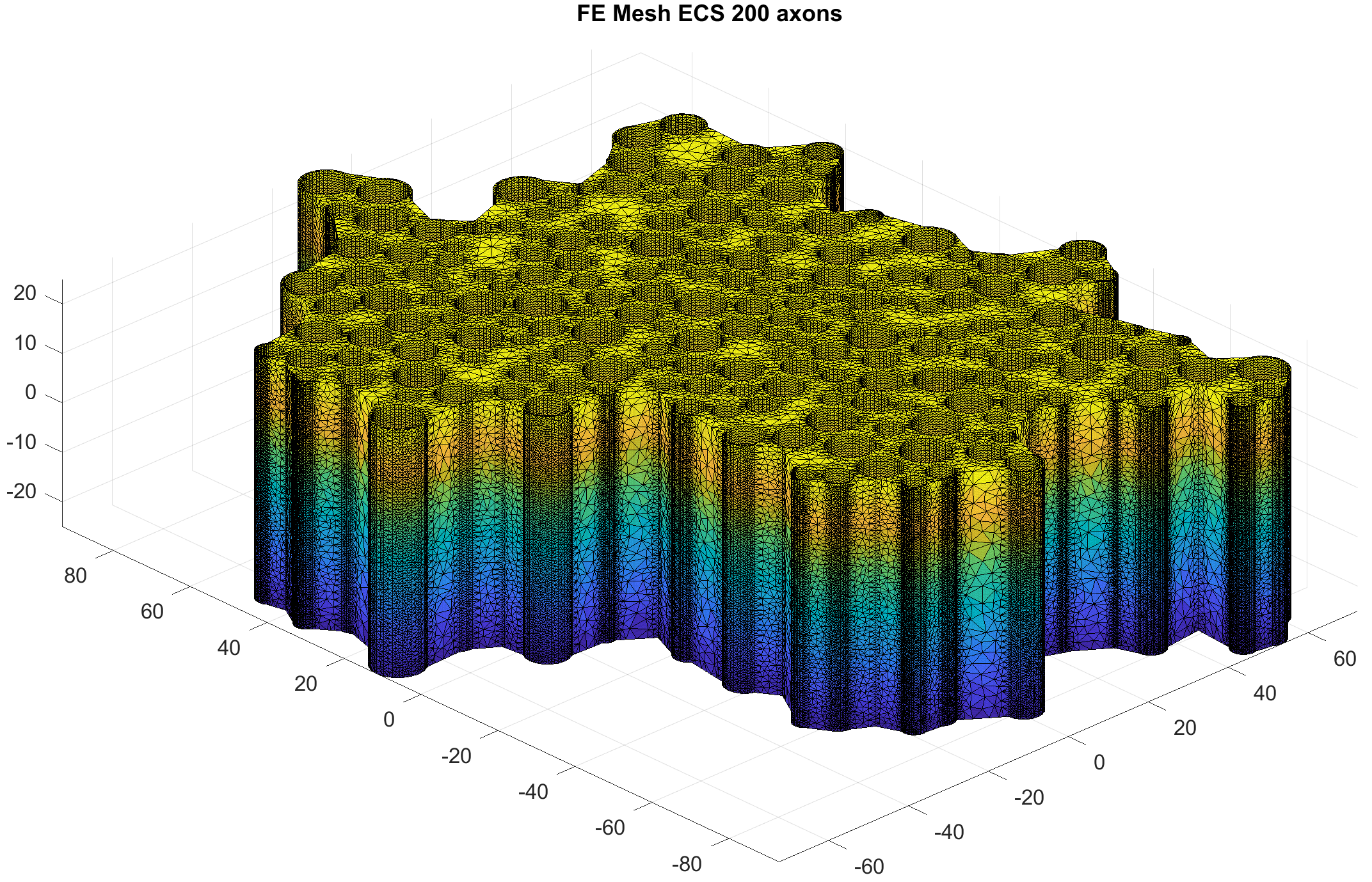
   Figure 12: The geometry is ECC200axons. This finite elements mesh size is ($n_{nodes}=846298,n_{elem}=2997386$)

   The dMRI experimental parameters are the following:

   • the diffusion coefficient is $2\times 10^{-3}\,\text{mm}^{2}/\text{s}$;

   • the diffusion-encoding sequence is PGSE ($\delta=10\text{ms}$, $\Delta=13\text{ms}$);

   • 8 b-values: $b=\{0,100,500,1000,2000,3000,6000,10000\}\,\text{s/mm}^{2}$;

   • 1 gradient direction: $[1,1,0]$.

   The SpinDoctor simulations were done using one compartment. The boundary of compartment is subject to impermeable boundary conditions. We took the surface triangulations associated with the finite element mesh for the SpinDoctor simulations and used them as the input PLY files for Camino. Camino is called with the command datasynth. The options of Camino that are relevant to the simulations in the above three geometries are the following:

   • -walkers ${N}: $N$ is the number of walkers ;

   • -tmax ${T}: $T$ is the number of time steps;

   • -p ${P}: $P$ is the probability that a spin will step through a barrier. We set $P$ to zero;

   • -voxels 1: using 1 voxel for the experiment;

   • -initial intra: random walkers are placed uniformly inside the geometry and none outside of it; In the case of the extra-cellular space, intra means inside the geometry, with the geometry representing the extracellular space;

   • -voxelsizefrac 1: the signal is computed using all the spins inside the geometry described by the PLY file, and not just in a center region;

   • -diffusivity 2E-9: the diffusion coefficient ($m^{2}/s$);

   • -meshsep ${xsep} ${ysep} ${zsep}: specifies the seperation between bounding box for mesh substrates. We used a box that fully contains the geometry described by the PLY file;

   • -substrate ply: mesh substrates are constructed using a PLY file;

   • -plyfile ${plyfile}: the name of the PLY file. We wrote a MATLAB function that outputs the list of triangles that make up the boundary of the finite element mesh and formatted it as a PLY file. We note these triangles form a surface triangulation;

   6.1 ECS of 400 axons

   SpinDoctor was run with the following 3 sets of simulation parameters:

   1. $rtol=10^{-3}$, $atol=10^{-6}$, $Htetgen=0.5$;

   2. $rtol=10^{-3}$, $atol=10^{-6}$, $Htetgen=1$;

   3. $rtol=10^{-3}$, $atol=10^{-6}$, $Htetgen=-1$;

      For this geometry, $Htetgen=-1$ gives finite elements mesh size ($n_{nodes}=53280,n_{elem}=125798$). $Htetgen=1$ gives finite elements mesh size ($n_{nodes}=58018,n_{elem}=139582$). $Htetgen=0.5$ gives finite elements mesh size ($n_{nodes}=70047,n_{elem}=177259$).

      Camino was run with the following 2 sets of simulation parameters:

      1. $N=1000$, $T=200$;

      2. $N=4000$, $T=800$;

         The reference signals are SpinD Simul 6.1-1, the SpinDoctor signals computed on the finest FE mesh ($Htetgen=0.5$).

         We computed the signal differences between the reference simulations and the 2 remaining SpinDoctor simulations as well as the two Camino signals:

         $$E(b)=\left|\frac{S(b)}{S(0)}-\frac{S^{ref}(b)}{S^{ref}(0)}\right|\times 100.$$ (17)

         In Figure 13 we see $E(b)$ for the SpinDoctor simulation on the coarsest mesh ($Htetgen=-1$) is less than $0.4\%$ for all b-values and for the SpinDoctor simulation on the mesh ($Htetgen=1$) it is less than $0.2\%$. The Camino simulation with ($N=1000$, $T=200$) has a signal difference of 1.9% for b-value up to $2000\,\text{s/mm}^{2}$, and the Camino simulation with ($N=4000$, $T=800$) has a signal difference of 0.7% for b-value up to $2000\,\text{s/mm}^{2}$. However, for b-value $b=3000\,\text{s/mm}^{2}$ and greater, it seems the first Camino simulation is closer to the reference signal than the second Camino simulation. It likely means that 4000 spins and 800 time steps are not enough to achieve signal convergence at higher b-values. In fact, they are below the recommended values for Monte-Carlo simulations [26], but we chose them to keep the Camino simulations running within a reasonable amount of time. On the other hand, the refinement of the FE mesh for the SpinDoctor achieves convergence for all b-values up to 10000$\,\text{s/mm}^{2}$. There is a significant increase of the computational time of SpinDoctor as the diffusion-encoding amplitude is increased from 0.03 T/m to 0.37 T/m. At the finest mesh, the computational time increased from 35 seconds to 200 seconds. At the coarsest mesh, the computational time increased from 20 seconds to 115 seconds. This is due to the fact that at higher gradient amplitudes, the magnetization is more oscillatory, so to achieve a fixed ODE solver tolerance, smaller time steps are needed.

         

         

         

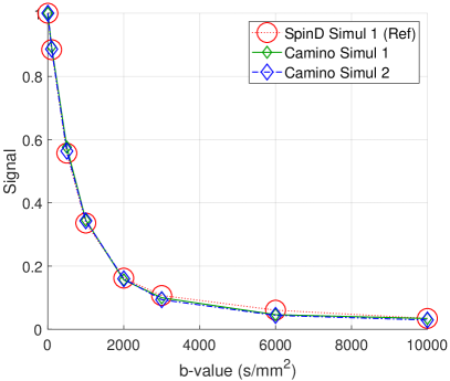
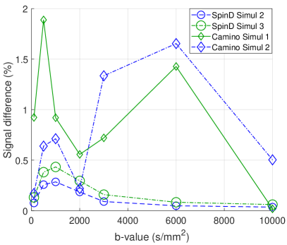
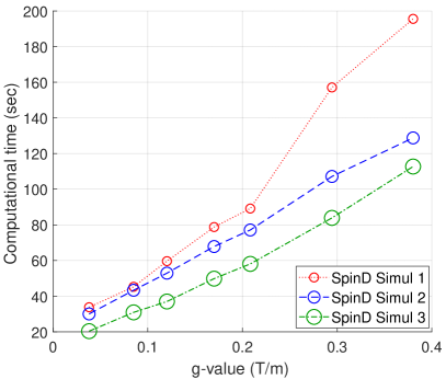
         Figure 13: The geometry is ECS400axons. Top: SpinD Simul 1 is the reference signal, compared to two Camino simulations. Bottom left: the signal difference between the reference simulation and two SpinDoctor simulations and two Camino simulations. Bottom right: the computational times of SpinDoctor simulations as a function of the gradient amplitude. The diffusion coefficient is $2\times 10^{-3}\,\text{mm}^{2}/\text{s}$; The diffusion-encoding sequence is PGSE ($\delta=10\text{ms}$, $\Delta=13\text{ms}$); The gradient direction is $[1,1,0]$. SpinD Simul 1: $rtol=10^{-3}$, $atol=10^{-6}$, $Htetgen=0.5$; SpinD Simul 2: $rtol=10^{-3}$, $atol=10^{-6}$, $Htetgen=1$; SpinD Simul 3: $rtol=10^{-3}$, $atol=10^{-6}$, $Htetgen=-1$; Camino Simul 1: $N=1000$, $T=200$; Camino Simul 2: $N=4000$, $T=800$;

         In Table 9 we show the total computational time to compute the dMRI signals at the 8 b-values for 2 SpinDoctor and 2 Camino simulations. We also include the time for Camino to place the initial spins in the geometry described by the PLY file. We include in the Table the maximum signal differences for b-values up to $2000\,\text{s/mm}^{2}$ instead of all the b-values because Camino is not convergent for b-values greater than $3000\,\text{s/mm}^{2}$. We see that at a similar level of signal difference ($0.4\%$ for SpinDoctor versus $0.7\%$ for Camino), the total computational time of SpinDoctor (438 seconds) is more than 100 times faster than Camino (59147 seconds).

         ECS400axons	SpinDoctor		Camino
         	Htet = -1	Htet = 0.5	$T=200$	$T=800$
         Degrees	53280 nodes	70047 nodes	1000 spins	4000 spins
         of freedom	125798 elements	177259 elements
         Max signal difference	0.4%	Ref signal	1.9%	0.7%
         ($b\leq 2000\,\text{s/mm}^{2}$)
         Initialization time (sec)			69	305
         Solve time (sec), 8 bvalues	438	667	3949	58842
         Total time (sec)	438	667	4018	59147

         Table 9: The geometry is ECS400axons. The total computational times (in seconds) to simulate the dMRI signal at 8 b-values using SpinDoctor and Camino. The initialization time is the time for Camino to place initial spins inside the geometry described by the PLY file. The b-values simulated are $b=\{0,100,500,1000,2000,3000,6000,10000\}\,\text{s/mm}^{2}$. The maximum signal differences are given for b-values up to $2000\,\text{s/mm}^{2}$ because Camino is not convergent for b-values greater than $3000\,\text{s/mm}^{2}$. The diffusion coefficient is $2\times 10^{-3}\,\text{mm}^{2}/\text{s}$; The diffusion-encoding sequence is PGSE ($\delta=10\text{ms}$, $\Delta=13\text{ms}$); The gradient direction is $[1,1,0]$.

         6.2 Dendrite branch

         SpinDoctor was run with the following 2 sets of simulation parameters:

         1. $rtol=10^{-3}$, $atol=10^{-6}$;

         2. $rtol=10^{-2}$, $atol=10^{-4}$;

            The finite elements mesh was generated by an external package and imported into SpinDoctor. The finite elements mesh size is ($n_{nodes}=24651,n_{elem}=91689$). We do not refine the FE mesh, rather, we vary the ODE solve tolerances in the SpinDoctor simulations.

            Camino was run with the following 3 sets of simulation parameters:

            1. $N=1000$, $T=200$;

            2. $N=2000$, $T=400$;

            3. $N=4000$, $T=800$;

               The reference signal is SpinD Simul 6.2-1, the SpinDoctor signal with the higher ODE solve tolerances ($rtol=10^{-3}$, $atol=10^{-6}$).

               In Figure 14 we see the signal difference $E(b)$ for the SpinDoctor simulation with the bigger ODE solve tolerances ($rtol=10^{-2}$, $atol=10^{-4}$) is less than $0.6\%$ for all b-values. The Camino simulation with ($N=1000$, $T=200$) has a maximum signal difference of 6.4%, the Camino simulation with ($N=4000$, $T=800$) has a maximum signal difference of 1.0%. As the gradient amplitude is increased from 0.03 T/m to 0.37 T/m, at the larger ODE solve tolerances, the computational time increased from 5 seconds to 17 seconds. At smaller ODE solve tolerances, the computational time increased from 7 seconds to 42 seconds. Again, this increase is due to the fact that at higher gradient amplitudes, the magnetization is more oscillatory, so to achieve a fixed ODE solver tolerance, smaller time steps are needed. In Table 10 we see for the same level of accuracy ($0.6\%$ for SpinDoctor and and $1\%$ for Camino), SpinDoctor (109 seconds) is 400 times faster than Camino (43918 seconds).

               

               

               

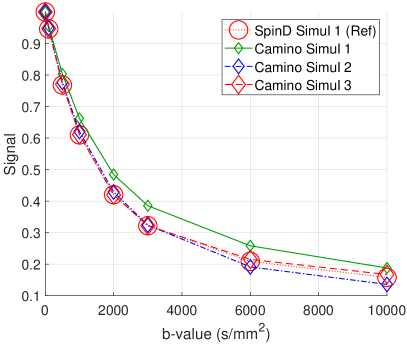
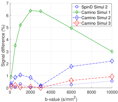
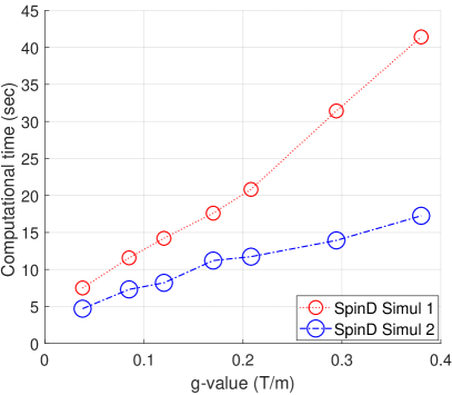
               Figure 14: The geometry is DendriteBranch. Top: SpinD Simul 1 is the reference signal, compared to three Camino simulations. Bottom left: the signal difference between the reference simulation and a SpinDoctor simulation and three Camino simulations. Bottom right: the computational times of SpinDoctor simulations as a function of the gradient amplitudes. The diffusion coefficient is $2\times 10^{-3}\,\text{mm}^{2}/\text{s}$; The diffusion-encoding sequence is PGSE ($\delta=10\text{ms}$, $\Delta=13\text{ms}$); The gradient direction is $[1,1,0]$. SpinD Simul 1: $rtol=10^{-3}$, $atol=10^{-6}$; SpinD Simul 2: $rtol=10^{-2}$, $atol=10^{-4}$; Camino Simul 1: $N=1000$, $T=200$; Camino Simul 2: $N=2000$, $T=400$; Camino Simul 3: $N=4000$, $T=800$;

               $Dendrite$	SpinDoctor		Camino
               $Branch$	$rtol=10^{-2}$	$rtol=10^{-3}$	$T=200$	$T=400$	$T=800$
               Degrees	24651 nodes		1000 spins	2000 spins	4000 spins
               of freedom	91689 elements
               Max signal difference	0.6%	Ref signal	6.4%	2.2%	1.0%
               Initialization time (sec)			5897	11739	23702
               Solve time (sec), 8 bvalues	109	207	1336	5138	20216
               Total time (sec)	109	207	7233	16877	43918

               Table 10: The geometry is DendriteBranch. The total computational times in seconds to simulate the dMRI signal at 8 b-values using SpinDoctor and Camino. The initialization time is the time for Camino to place initial spins inside the geometry described by the PLY file. The b-values simulated are $b=\{0,100,500,1000,2000,3000,6000,10000\}\,\text{s/mm}^{2}$. The diffusion coefficient is $2\times 10^{-3}\,\text{mm}^{2}/\text{s}$; The diffusion-encoding sequence is PGSE ($\delta=10\text{ms}$, $\Delta=13\text{ms}$); The gradient direction is $[1,1,0]$.

               6.3 Three dimensional ECS of 200 axons

               Due to computational time limitations, we only computed 4 b-values, $b=\{0,100,500,1000\}\,\text{s/mm}^{2}$, for the geometry ECS200axons (see Figure 12 for the finite element mesh).

               SpinDoctor was run with the following 2 sets of simulation parameters:

               1. $rtol=10^{-3}$, $atol=10^{-6}$, $Htetgen=-1$

               2. $rtol=10^{-3}$, $atol=10^{-6}$, $Htetgen=0.3$.

                  For this geometry, $Htetgen=-1$ gives finite elements mesh size ($n_{nodes}=846298,n_{elem}=2997386$). $Htetgen=0.3$ gives finite elements mesh size ($n_{nodes}=1017263,n_{elem}=3950572$).

                  The difference inthe signals between the two simulations is less than $0.35\%$ (not plotted), meaning the FE meshes are fine enough to produce accurate signals. In Table 11, we see that using about 846K nodes required 1.8 hours at $b=100\,\text{s/mm}^{2}$, 2.7 hours at $b=500\,\text{s/mm}^{2}$, 3.3 hours at $b=1000\,\text{s/mm}^{2}$. We did not use Camino for ECS200axons due to the excessive time required by Camino.

                  ECS200 axons	SpinDoctor
                  	Htet = -1	Htet = 0.3
                  Mesh	846298 nodes	1017263 nodes
                  	2997386 elements	3950572 elements
                  Max signal difference	0.35%	Ref signal
                  Solve time (sec), $b=100,500,1000\,\text{s/mm}^{2}$	(6611, 9620, 12107)	(16978, 23988, 32044)

                  Table 11: The geometry is ECS200axons. The computational times in seconds to simulate the dMRI signal at 3 b-values $b=\{100,500,1000\}\,\text{s/mm}^{2}$ using SpinDoctor. The times are listed separately for each b-value. The diffusion coefficient is $2\times 10^{-3}\,\text{mm}^{2}/\text{s}$; The diffusion-encoding sequence is PGSE ($\delta=10\text{ms}$, $\Delta=13\text{ms}$); The gradient direction is $[1,1,0]$.

                  6.4 SpinDoctor computational time

                  We collected the computational times of the SpinDoctor simulations for ECS400axons, DendriteBranch, and ECS200axons, that had the ODE solve tolerances ($rtol=10^{-3}$, $atol=10^{-6}$). In addition, for ECS400axons and DendriteBranch, we performed simulations for another PGSE sequence ($\delta=10\text{ms}$, $\Delta=23\text{ms}$).

                  Now we examine the computational time as a function of the finite element mesh size for those simulations with ODE solve tolerances ($rtol=10^{-3}$, $atol=10^{-6}$). There are 3 FE meshes of ECS400axons, 1 FE mesh of DendriteBranch, and 2 FE meshes of ECS200axons. In Figure 15 we plot the computational times to simulate the dMRI signal at two b-values ($b=100\,\text{s/mm}^{2}$ and $b=1000\,\text{s/mm}^{2}$) as a function of the number of FE nodes. We see at fewer than 100K finite element nodes, the SpinDoctor simulation time is less than 1 minute per b-value. At 1 million FE nodes, the SpinDoctor simulation time is about 4.7 hours for $b=100\,\text{s/mm}^{2}$ and 8.9 hours for $b=1000\,\text{s/mm}^{2}$.

                  

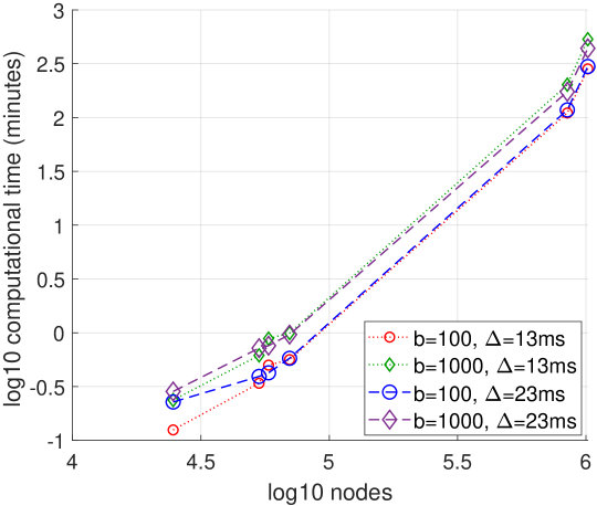
                  Figure 15: Computational times of SpinDoctor to simulate one b-value (either $b=100\,\text{s/mm}^{2}$ or $b=1000\,\text{s/mm}^{2}$). The x-axis gives log 10 of the number of finite elements nodes. The data include 3 FE meshes of ECS400axons, 1 FE mesh of DendriteBranch, and 2 FE meshes of ECS200axons. The y-axis gives the log 10 of the comptational time in minutes. Below $y=0$ are computational times that are less than one minute. The two sequences simulated are PGSE sequence ($\delta=10\text{ms}$, $\Delta=13\text{ms}$) and PGSE sequence ($\delta=10\text{ms}$, $\Delta=23\text{ms}$). The diffusion coefficient is $2\times 10^{-3}\,\text{mm}^{2}/\text{s}$; The gradient direction is $[1,1,0]$.

                  7 SpinDoctor permeability and Monte-Carlo transmission probability

                  Here we illustrate the link between the membrane permeability of Spindoctor and the transmission probability of crossing a membrane in the Camino simulation. The geometry is the following:

                  • Permeable Sphere involves uniformly placed initial spins inside a sphere of radius $5\mu\text{m}$, subject to permeable interface condition on the surface of the sphere, with permeability coefficient $\kappa$. No spins are initially placed outside of this sphere. In the SpinDoctor simulation, this sphere is enclosed inside a sphere of diameter $30\mu\text{m}$, subject to impermeable boundary condition on the outermost interface. In the Camino simulation, this sphere is enclosed in a box of side length $30\mu\text{m}$, subject to periodic boundary conditions. The inner sphere is far enough from the outer sphere in SpinDoctor and from the outer box in Camino so that there is no influence of the outer surface during the simulated diffusion times.

                  The dMRI experimental parameters are the following:

                  • the diffusion coefficient in all compartments is $2\times 10^{-3}\,\text{mm}^{2}/\text{s}$;

                  • the diffusion-encoding sequence is PGSE ($\delta=10\text{ms}$, $\Delta=13\text{ms}$);

                  • 8 b-values: $b=\{0,100,500,1000,2000,3000,6000,10000\}\,\text{s/mm}^{2}$;

                  • 1 gradient direction: $[1,1,0]$.

                  SpinDoctor was run with the following 3 sets of simulation parameters:

                  1. $rtol=10^{-3}$, $atol=10^{-6}$, $Htetgen=0.5$;

                  2. $rtol=10^{-3}$, $atol=10^{-6}$, $Htetgen=1$;

                  3. $rtol=10^{-3}$, $atol=10^{-6}$, $Htetgen=-1$;

                     For this geometry, $Htetgen=-1$ gives finite elements mesh size ($n_{nodes}=46384,n_{elem}=196920$). $Htetgen=1$ gives finite elements mesh size ($n_{nodes}=49618,n_{elem}=218007$). $Htetgen=0.5$ gives finite elements mesh size ($n_{nodes}=52803,n_{elem}=237613$).

                     Camino was run with the following 2 sets of simulation parameters:

                     1. $N=4000$, $T=800$;

                     2. $N=8000$, $T=3200$;

                        The reference signal is SpinD Simul 7-1, the SpinDoctor signal on the finest FE mesh.

                        In [57], there is a discussion about the transmission probability of random walkers as they encounter a permeable membrane with permeability $\kappa$. The formula found in that paper is (for three dimensions)

                        $$P_{EX}=C_{dim}\frac{\kappa}{\sigma}\sqrt{2\,dim\,\sigma\,\delta t},\quad C_{dim}=\frac{2}{3},\quad dim=3,$$ (18)

                        $\sigma$ being the intrinsic diffusion coefficient, $\delta t$ is the time step.

                        In Figure 16 we show the three SpinDoctor simulations at $\kappa=10^{-5}\,\text{m}/\text{s}$ and the two Camino simulations using the above formula for $P_{EX}$. We considered the SpinDoctor signal computed on the finest FE mesh as the reference signal and we computed the signal differences between the reference signal and the other two SpinDoctor signals and the Camino signals. We see that the Camino signals approach the reference signal as the number of spins and times steps in Camino are increased, the maximum difference decreasing from 3.8% to 2.4%. The SpinDoctor signals have signal differences of less than 0.5% and 0.1%, respectively.

                        

                        

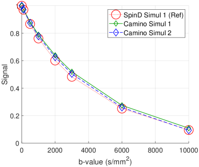
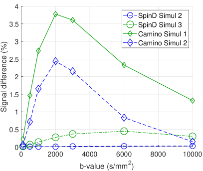
                        Figure 16: The Permeable Sphere example involves uniformly placed initial spins inside a sphere of radius $5\mu\text{m}$, subject to permeable interface condition on the surface of the sphere, with permeability coefficient $\kappa=10^{-5}\,\text{m}/\text{s}$. Left: the SpinDoctor simulation on the finest mesh as the reference signal and two Camino signals. Right: the signal difference between the reference signal and two SpinDoctor simulations and two Camino simulations. SpinD Simul 1: $rtol=10^{-3}$, $atol=10^{-6}$, $Htetgen=0.5$; SpinD Simul 2: $rtol=10^{-3}$, $atol=10^{-6}$, $Htetgen=1$; SpinD Simul 3: $rtol=10^{-3}$, $atol=10^{-6}$, $Htetgen=-1$; Camino Simul 1: $N=4000$, $T=800$; Camino Simul 2: $N=8000$, $T=3200$; The diffusion coefficient in all compartments is $2\times 10^{-3}\,\text{mm}^{2}/\text{s}$; The diffusion-encoding sequence is PGSE ($\delta=10\text{ms}$, $\Delta=13\text{ms}$); The gradient direction is $[1,1,0]$.

                        8 Extensions of SpinDoctor

                        Here we mention two extensions in the functionalities of SpinDoctor that are planned for a future release.

                        8.1 Non-standard diffusion-encoding sequences

                        Given the interest in nonstandard diffusion sequences beyond PGSE and OGSE, such as double diffusion encoding (see [58, 59, 60, 61]) and multidimensional diffusion encoding (see [62]), it is natural that SpinDoctor should easily support arbitrary diffusion-encoding sequences. Besides the PGSE and the sine and cosine OGSE sequences that are provided in the SpinDoctor package, new sequences can be straightforwardly implemented by changing three files in the SpinDoctor package

                        • SRC/DMRI/seqprofile.m defines $f(t)$

                        • SRC/DMRI/seqintprofile.m defines the integral $F(t)=\int_{0}^{t}f(s)ds$

                        • SRC/DMRI/seqbvaluenoq.m defines the associated $b-$value.

                        In the example below, we simulate the double-PGSE (Eq. 19) sequence:

                        $$f(t)=\begin{cases}1,\quad&0\leq t\leq\delta,\\ -1,\quad&\Delta<t\leq\Delta+\delta,\\ 1,\quad&\tau\leq t\leq\delta+\tau,\\ -1,\quad&\Delta+\tau<t\leq\Delta+\delta+\tau,\\ 0,\quad&\text{otherwise.}\end{cases}$$ (19)

                        Here $\delta$ is the duration of the diffusion-encoding gradient pulse, $\Delta$ is the time delay between the start of the two pulses, and $\tau$ is the distance between the two pairs of pulses ($\tau\geq\delta+\Delta$). The geometry is made of cylindrical cells, the myelin layer, and the ECS (see Figure 7). In Figure 17 we show the dMRI signals for the PGSE ($\delta=10\text{ms},\Delta=13\text{ms}$) and dPGSE sequences ($\delta=10\text{ms},\Delta=13\text{ms},\tau=\delta+\Delta$), the diffusion-encoding direction is ${\bm{u_{g}}}=[1,1,1]$.

                        

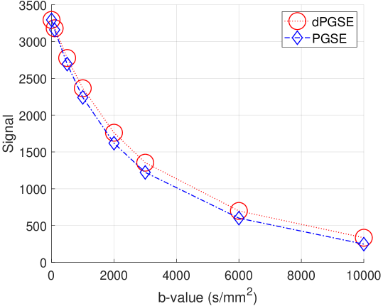
                        Figure 17: DMRI signals of the PGSE and the double PGSE diffusion-encoding sequences. The geometry is made of cylindrical cells, the myelin layer, and the ECS (see Figure 7). The diffusion coefficient in all compartments is $2\times 10^{-3}\,\text{mm}^{2}/\text{s}$ and the compartments do not experience spin exchange, with all permeability coefficients set to zero. The diffusion-encoding sequeces are PGSE ($\delta=10\text{ms},\Delta=13\text{ms}$) and dPGSE sequences ($\delta=10\text{ms},\Delta=13\text{ms},\tau=\delta+\Delta$), the diffusion-encoding direction is ${\bm{u_{g}}}=[1,1,1]$.

                        8.2 $T_{2}$ relaxation

                        When $T_{2}-$relaxation is considered, the Bloch-Torrey PDE (Eq. 1) takes the following form

                        $$\frac{\partial}{\partial t}{M^{in}_{i}({\bm{x}},t)} =-I\gamma f(t){\bm{g}}\cdot{\bm{x}}\,M^{in}_{i}({\bm{x}},t)-\frac{M^{in}}{T^{in}_{2}}+\nabla\cdot(\sigma^{in}\nabla M^{in}_{i}({\bm{x}},t)), {\bm{x}}\in\Omega^{in}_{i},$$ (20)

                        $$\frac{\partial}{\partial t}{M^{out}_{i}({\bm{x}},t)} =-I\gamma f(t){\bm{g}}\cdot{\bm{x}}\,M^{out}_{i}({\bm{x}},t)-\frac{M^{out}}{T^{out}_{2}}+\nabla\cdot(\sigma^{out}\nabla M^{out}_{i}({\bm{x}},t)),\; {\bm{x}}\in\Omega^{out}_{i},$$ (21)

                        $$\frac{\partial}{\partial t}{M^{e}({\bm{x}},t)} =-I\gamma f(t){\bm{g}}\cdot{\bm{x}}\,M^{e}({\bm{x}},t)-\frac{M^{e}}{T^{e}_{2}}+\nabla\cdot(\sigma^{e}\nabla M^{e}({\bm{x}},t)), {\bm{x}}\in\Omega^{e},$$ (22)

                        We plan to incorporate $T_{2}$ relaxation effects in the next official release of SpinDoctor. In the meantime, this additional functionality can be found in a development branch of SpinDoctor available on GitHub. The source code in this development branch allows the ability to add relaxation, with different relaxivities in the different compartments [63, 64].

                        $T_{2}$ relaxation is incorporated using the format $T_{2}=[T_{2}^{in},T_{2}^{out},T_{2}^{e}]$ where $T_{2}^{in},T_{2}^{out},T_{2}^{e}$ are the $T_{2}$ values for the three compartments, respectively. To verify the correctness of our implementation, we check the following. Let $S_{\text{No-T2}}(b)$ be the signal without $T_{2}$ effects. If there is no exchange between compartments, then the $T_{2}$ effects can be cancelled from the signals in the three compartments that include $T_{2}$ effects in the following way:

                        $${S_{cancel}}(b) =\frac{S^{in}(b)}{e^{-\frac{TE}{T_{2}^{in}}}}+\frac{S^{out}(b)}{e^{-\frac{TE}{T_{2}^{out}}}}+\frac{S^{e}(b)}{e^{-\frac{TE}{T_{2}^{e}}}}.$$ (23)

                        In Fig. 18, we compare $S_{\text{No-T2}}(b)$ with $S(b)$ where $T_{2}=[50\text{ms},20\text{ms},100\text{ms}]$, for the PGSE sequences ($\delta=10\text{ms},\Delta=13\text{ms}$) and ${\bm{u_{g}}}=[1,1,1]$. We also compute ${S_{cancel}}(b)$, using Eq. 23. The geometry (see Figure 7) is made of cylindrical cells, the myelin layer, and the ECS. The $T_{2}$ effects on the signal $S(b)$ are clearly seen. The $T_{2}$ effects are completely canceled out using Eq. (23).

                        

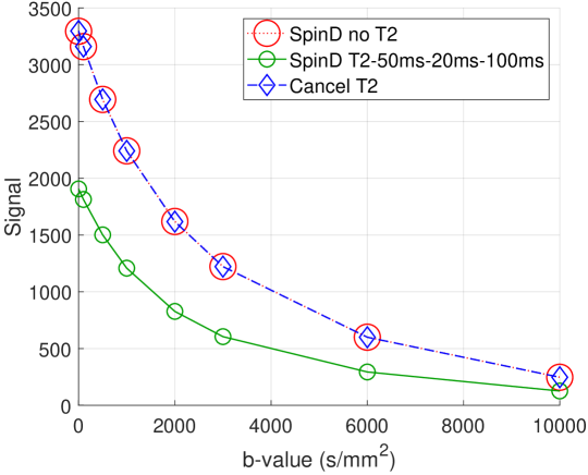
                        Figure 18: DMRI signal including $T_{2}=[50\text{ms},20\text{ms},100\text{ms}]$ relaxation is lower than the signal without relaxation effects (”no T2”). The $T_{2}$ effects are completely canceled out using Eq. 23 so that the curve ”cancel T2” coincides with the no relaxation signal. The geometry is made of cylindrical cells, the myelin layer, and the ECS (see Figure 7). The diffusion coefficient in all compartments is $2\times 10^{-3}\,\text{mm}^{2}/\text{s}$ and the compartments do not experience spin exchange, with all permeability coefficients set to zero. The diffusion-encoding sequece is PGSE ($\delta=10\text{ms},\Delta=13\text{ms}$), the diffusion-encoding direction is ${\bm{u_{g}}}=[1,1,1]$.

                        9 Discussion

                        Built upon MATLAB, SpinDoctor is a software package that seeks to reduce the work required to perform numerical simulations for dMRI for prototyping purposes. There have been software packages for dMRI simulation that implements the random walkers approach. A detailed comparison of the Monte-Carlo/random walkers approach with the FEM approach is beyond the scope of this paper. SpinDoctor offers an alternative, solving the same physics problem using PDEs.

                        After surveying other works on dMRI simulations, we saw a need to have a simulation toolbox that provides a way to easily define geometrical configurations. In SpinDoctor we have tried to offer useful configurations, without being overly general. Allowing too much generality in the geometrical configurations would have made code robustness very difficult to achieve due to the difficulties related to problems in computational geometry (high quality surface triangulation, robust FE mesh generation). The geometrical configuration routines provided by SpinDoctor are a helpful front end, to enable dMRI researchers to get started quickly to perform numerical simulations. Those users who already have a high quality surface triangulation can use the other parts of SpinDoctor without passing through this front end.

                        The bulk of SpinDoctor is the numerical solutions of two PDEs. When one is only interested in the ADC, then computing the HADC model is the good option. When one is interested in higher order behavior in the dMRI signal, then the BTPDE model is a good option for accessing high b-value behavior.

                        Because time stepping methods for semi-discretized linear systems arising from finite element discretization is a well-studied subject in the mathematical literature, the ODE solvers implemented in MATLAB already optimize for such linear systems. For example, the mass matrix is passed into the ODE solver as an optional parameter so as to avoid explicit matrix inversion. In addition, the ODE solution is guaranteed to stay within a user-requested residual tolerance. We believe this type of optimization and error control is clearly advantageous over simulation codes that do not have it.

                        To mimic the phenomenon where the water molecules can enter and exit the computational domain, the pseudo-periodic boundary conditions were implemented in [33, 34, 35]. At this stage, we have chosen not to implement this in SpinDoctor, instead, spins are not allowed to leave the computational domain. Implementing pseudo-periodic boundary conditions would make the code more complicated, and it remains to be seen if it is a desired feature among potential users. If it is, then it could be part of a future development.

                        The twising and bending of the canonical configuration is something unique to SpinDoctor. It removes many computational geometry difficulties by meshing first the canonical configuration before deforming the FE mesh via an analytical coordinate transformation. This is a way to simulate fibers that are not parallel, that bend, for example. For fibers that disperse, perhaps more complicated analytical coordinate transformations can be performed on the canonical configuration to mimic that situation. This is a possible future direction to explore.

                        SpinDoctor depends on MATLAB for the ODE solve routines as well as for the computational geometry routines to produce the tight wrap ECS. To implement SpinDoctor outside of MATLAB would require replacing these two sets of MATLAB routines. Other routines of SpinDoctor can be easily implemented in another programming language.

                        SpinDoctor can be downloaded at https://github.com/jingrebeccali/SpinDoctor.

                        In summary, we have validated SpinDoctor simulations using reference signals from the Matrix Formalism method, in particular in the case of permeable membranes. We then compared SpinDoctor with the Monte-Carlo simulations produced by the publicly available software package Camino Diffusion MRI Toolkit [26]. We showed that the membrane permeability of SpinDoctor can be straightforwardly linked to the transmission probability in Monte-Carlo simulations. For numerous examples, it was seen that the SpinDoctor and the Camino simulations can be made close to each other if one increases the degrees of freedom (the finite element mesh size for SpinDoctor and the number of spins for Camino) and increase the accuracy of the time stepping (by tightening the ODE solve tolerances in SpinDoctor and by increasing the number of time steps in Camino).

                        At high gradient amplitudes, the ocsillatory nature of the magnetization requires the use of smaller time steps to maintain accuracy. For this reason, the computational time to simulate the dMRI signal at high gradient amplitudes must be longer than at low gradient amplitudes. This adaptivity in the time stepping as a function of gradient amplitude is done automatically in SpinDoctor.

                        We have computed the dMRI signals on several complicated geometries on a stand-alone computer. For these examples, we have shown that SpinDoctor can be more than 100 times faster than Camino. Of course, in simple configurations such as straight, parallel cylinders, it is much more efficient to use an analytical representation of the diffusion environment rather than a triangulated mesh in Camino. In addition, some recent implementations of random walk simulations [65, 66] should be faster than Camino.

                        With a finite element mesh of 100K nodes, SpinDoctor takes less than one minute per b-value. At 1 million finite element nodes, limited computer memory resulted in a computational time 4.7 hours for $b=100\,\text{s/mm}^{2}$ and 8.9 hours for $b=1000\,\text{s/mm}^{2}$. This issue will be taken into account in the future with high performance computing techniques in MATLAB and on other platforms. One of our recent works [40] is promising for this purpose.

                        We also illustrated several extensions of SpinDoctor functionalities, including the incorporation of $T_{2}$ relaxation, the simulation of non-standard diffusion-encoding sequences. We note the dendrite branch example illustrates SpinDoctor’s ability to import and use externally generated meshes provided by the user. This capability will be very useful given the most recent developments in simulating ultra-realistic virtual tissues [67, 65].

                        10 Conclusion

                        This paper describes a publicly available MATLAB toolbox called SpinDoctor that can be used to solve the BTPDE to obtain the dMRI signal and to solve the diffusion equation of the HADC model to obtain the ADC. SpinDoctor is a software package that seeks to reduce the work required to perform numerical simulations for dMRI for prototyping purposes.

                        SpinDoctor provides built-in options of including spherical cells with a nucleus, cylindrical cells with a myelin layer, an extra-cellular space enclosed either in a box or in a tight wrapping around the cells. The deformation of canonical cells by bending and twisting is implemented via an analytical coordinate transformation of the FE mesh. Permeable membranes for the BTPDE is implemented using double nodes on the compartment interfaces. Built-in diffusion-encoding pulse sequences include the Pulsed Gradient Spin Echo and the Ocsillating Gradient Spin Echo. Error control in the time stepping is done using built-in MATLAB ODE solver routines.

                        User feedback to improve SpinDoctor is welcomed.

                        Acknowledgment

                        The authors gratefully acknowledge the French-Vietnam Master in Applied Mathematics program whose students (co-authors on this paper, Van-Dang Nguyen, Try Nguyen Tran, Bang Cong Trang, Khieu Van Nguyen, Vu Duc Thach Son, Hoang An Tran, Hoang Trong An Tran, Thi Minh Phuong Nguyen) have contributed to the SpinDoctor project during their internships in France in the past several years, as well as the Vice-Presidency for Marketing and International Relations at Ecole Polytechnique for financially supporting a part of the students’ stay. Jan Valdman was supported by the Czech Science Foundation (GACR), through the grant GA17-04301S. Van-Dang Nguyen was supported by the Swedish Energy Agency, Sweden with the project ID P40435-1 and MSO4SC with the grant number 731063.

References

- [1] E. L. Hahn, Spin echoes, Phys. Rev. 80 (1950) 580–594.
- [2] E. O. Stejskal, J. E. Tanner, Spin diffusion measurements: Spin echoes in the presence of a time-dependent field gradient, The Journal of Chemical Physics 42 (1) (1965) 288–292. doi:10.1063/1.1695690.
- [3] D. L. Bihan, E. Breton, D. Lallemand, P. Grenier, E. Cabanis, M. Laval-Jeantet, MR imaging of intravoxel incoherent motions: application to diffusion and perfusion in neurologic disorders., Radiology 161 (2) (1986) 401–407, pMID: 3763909.
- [4] M. D. Does, E. C. Parsons, J. C. Gore, Oscillating gradient measurements of water diffusion in normal and globally ischemic rat brain, Magn. Reson. Med. 49 (2) (2003) 206–215. doi:10.1002/mrm.10385.
- [5] J. H. Jensen, J. A. Helpern, A. Ramani, H. Lu, K. Kaczynski, Diffusional kurtosis imaging: The quantification of non-Gaussian water diffusion by means of magnetic resonance imaging, Magnetic Resonance in Medicine 53 (6) (2005) 1432–1440. doi:10.1002/mrm.20508.
-
[6]
D. S. Tuch, T. G. Reese, M. R. Wiegell, N. Makris, J. W. Belliveau, V. J.
Wedeen, High
angular resolution diffusion imaging reveals intravoxel white matter fiber
heterogeneity, Magnetic Resonance in Medicine 48 (4) (2002) 577–582.
arXiv:https://onlinelibrary.wiley.com/doi/pdf/10.1002/mrm.10268,
doi:10.1002/mrm.10268.
URL https://onlinelibrary.wiley.com/doi/abs/10.1002/mrm.10268 -
[7]
Y. Assaf, T. Blumenfeld-Katzir, Y. Yovel, P. J. Basser,
Axcaliber:
A method for measuring axon diameter distribution from diffusion MRI,
Magnetic Resonance in Medicine 59 (6) (2008) 1347–1354.
arXiv:https://onlinelibrary.wiley.com/doi/pdf/10.1002/mrm.21577,
doi:10.1002/mrm.21577.
URL https://onlinelibrary.wiley.com/doi/abs/10.1002/mrm.21577 -
[8]
D. C. Alexander, P. L. Hubbard, M. G. Hall, E. A. Moore, M. Ptito, G. J.
Parker, T. B. Dyrby,
Orientationally
invariant indices of axon diameter and density from diffusion MRI,
NeuroImage 52 (4) (2010) 1374–1389.
URL http://www.sciencedirect.com/science/article/pii/S1053811910007755 -
[9]
H. Zhang, P. L. Hubbard, G. J. Parker, D. C. Alexander,
Axon
diameter mapping in the presence of orientation dispersion with diffusion
MRI, NeuroImage 56 (3) (2011) 1301–1315.
URL http://www.sciencedirect.com/science/article/pii/S1053811911001376 -
[10]
H. Zhang, T. Schneider, C. A. Wheeler-Kingshott, D. C. Alexander,
NODDI:
Practical in vivo neurite orientation dispersion and density imaging of the
human brain, NeuroImage 61 (4) (2012) 1000–1016.
URL http://www.sciencedirect.com/science/article/pii/S1053811912003539 - [11] L. M. Burcaw, E. Fieremans, D. S. Novikov, Mesoscopic structure of neuronal tracts from time-dependent diffusion, NeuroImage 114 (2015) 18 – 37. doi:10.1016/j.neuroimage.2015.03.061.
- [12] M. Palombo, C. Ligneul, J. Valette, Modeling diffusion of intracellular metabolites in the mouse brain up to very high diffusion-weighting: Diffusion in long fibers (almost) accounts for non-monoexponential attenuation, Magnetic Resonance in Medicine 77 (1) (2017) 343–350. doi:10.1002/mrm.26548.
- [13] M. Palombo, C. Ligneul, C. Najac, J. Le Douce, J. Flament, C. Escartin, P. Hantraye, E. Brouillet, G. Bonvento, J. Valette, New paradigm to assess brain cell morphology by diffusion-weighted MR spectroscopy in vivo, Proceedings of the National Academy of Sciences 113 (24) (2016) 6671–6676. arXiv:http://www.pnas.org/content/113/24/6671.full.pdf, doi:10.1073/pnas.1504327113.
- [14] L. Ning, E. Özarslan, C.-F. Westin, Y. Rathi, Precise inference and characterization of structural organization (picaso) of tissue from molecular diffusion, NeuroImage 146 (2017) 452 – 473. doi:10.1016/j.neuroimage.2016.09.057.
- [15] D. J. McHugh, F. Zhou, P. L. Hubbard Cristinacce, J. H. Naish, G. J. M. Parker, Ground truth for diffusion MRI in cancer: A model-based investigation of a novel tissue-mimetic material, in: S. Ourselin, D. C. Alexander, C.-F. Westin, M. J. Cardoso (Eds.), Information Processing in Medical Imaging, Springer International Publishing, Cham, 2015, pp. 179–190.
-
[16]
O. Reynaud,
Time-dependent
diffusion MRI in cancer: Tissue modeling and applications, Frontiers in
Physics 5 (2017) 58.
doi:10.3389/fphy.2017.00058.
URL https://www.frontiersin.org/article/10.3389/fphy.2017.00058 - [17] E. Fieremans, J. H. Jensen, J. A. Helpern, White matter characterization with diffusional kurtosis imaging, NeuroImage 58 (1) (2011) 177 – 188.
-
[18]
E. Panagiotaki, T. Schneider, B. Siow, M. G. Hall, M. F. Lythgoe, D. C.
Alexander,
Compartment
models of the diffusion MR signal in brain white matter: A taxonomy and
comparison, NeuroImage 59 (3) (2012) 2241–2254.
URL http://www.sciencedirect.com/science/article/pii/S1053811911011566 -
[19]
S. N. Jespersen, C. D. Kroenke, L. Astergaard, J. J. Ackerman, D. A.
Yablonskiy,
Modeling
dendrite density from magnetic resonance diffusion measurements, NeuroImage
34 (4) (2007) 1473–1486.
URL http://www.sciencedirect.com/science/article/pii/S1053811906010950 - [20] A. Ianuş, D. C. Alexander, I. Drobnjak, Microstructure imaging sequence simulation toolbox, in: S. A. Tsaftaris, A. Gooya, A. F. Frangi, J. L. Prince (Eds.), Simulation and Synthesis in Medical Imaging, Springer International Publishing, Cham, 2016, pp. 34–44.
-
[21]
I. Drobnjak, H. Zhang, M. G. Hall, D. C. Alexander,
The
matrix formalism for generalised gradients with time-varying orientation in
diffusion NMR, Journal of Magnetic Resonance 210 (1) (2011) 151 – 157.
doi:10.1016/j.jmr.2011.02.022.
URL http://www.sciencedirect.com/science/article/pii/S1090780711000838 -
[22]
M. Mercredi, M. Martin, Toward
faster inference of micron-scale axon diameters using Monte Carlo
simulations, Magnetic Resonance Materials in Physics, Biology and Medicine
31 (4) (2018) 511–530.
doi:10.1007/s10334-018-0680-1.
URL https://doi.org/10.1007/s10334-018-0680-1 -
[23]
G. Rensonnet, B. Scherrer, S. K. Warfield, B. Macq, M. Taquet,
Assessing
the validity of the approximation of diffusion-weighted-MRI signals from
crossing fascicles by sums of signals from single fascicles, Magnetic
Resonance in Medicine 79 (4) (2018) 2332–2345.
arXiv:https://onlinelibrary.wiley.com/doi/pdf/10.1002/mrm.26832,
doi:10.1002/mrm.26832.
URL https://onlinelibrary.wiley.com/doi/abs/10.1002/mrm.26832 - [24] B. D. Hughes, Random walks and random environments, Clarendon Press Oxford ; New York, 1995.
- [25] C.-H. Yeh, B. Schmitt, D. Le Bihan, J.-R. Li-Schlittgen, C.-P. Lin, C. Poupon, Diffusion microscopist simulator: A general monte carlo simulation system for diffusion magnetic resonance imaging, PLoS ONE 8 (10) (2013) e76626. doi:10.1371/journal.pone.0076626.
- [26] M. Hall, D. Alexander, Convergence and parameter choice for Monte-Carlo simulations of diffusion MRI, IEEE Transactions on Medical Imaging 28 (9) (2009) 1354 –1364. doi:10.1109/TMI.2009.2015756.
-
[27]
G. T. Balls, L. R. Frank, A
simulation environment for diffusion weighted MR experiments in complex
media, Magn. Reson. Med. 62 (3) (2009) 771–778.
URL http://dx.doi.org/10.1002/mrm.22033 -
[28]
K. V. Nguyen, E. H. Garzon, J. Valette,
Efficient
GPU-based Monte-Carlo simulation of diffusion in real astrocytes
reconstructed from confocal microscopy, Journal of Magnetic Resonance
(2018).
doi:10.1016/j.jmr.2018.09.013.
URL http://www.sciencedirect.com/science/article/pii/S1090780718302386 -
[29]
C. A. Waudby, J. Christodoulou,
GPU
accelerated Monte Carlo simulation of pulsed-field gradient NMR
experiments, Journal of Magnetic Resonance 211 (1) (2011) 67 – 73.
doi:https://doi.org/10.1016/j.jmr.2011.04.004.
URL http://www.sciencedirect.com/science/article/pii/S1090780711001376 -
[30]
H. Hagslatt, B. Jonsson, M. Nyden, O. Soderman,
Predictions
of pulsed field gradient NMR echo-decays for molecules diffusing in various
restrictive geometries. simulations of diffusion propagators based on a
finite element method, Journal of Magnetic Resonance 161 (2) (2003)
138–147.
URL http://www.sciencedirect.com/science/article/pii/S1090780702000393 - [31] N. Loren, H. Hagslatt, M. Nyden, A.-M. Hermansson, Water mobility in heterogeneous emulsions determined by a new combination of confocal laser scanning microscopy, image analysis, nuclear magnetic resonance diffusometry, and finite element method simulation, The Journal of Chemical Physics 122 (2) (2005) –. doi:10.1063/1.1830432.
-
[32]
B. F. Moroney, T. Stait-Gardner, B. Ghadirian, N. N. Yadav, W. S. Price,