Firing statistics in the bistable regime of neurons with homoclinic spike generation

Abstract

Abstract: Neuronal voltage dynamics of regularly firing neurons typically has one stable attractor: either a fixed point (like in the subthreshold regime) or a limit cycle that defines the tonic firing of action potentials (in the suprathreshold regime). In two of the three spike onset bifurcation sequences that are known to give rise to all-or-none type action potentials, however, the resting-state fixpoint and limit cycle spiking can coexist in an intermediate regime, resulting in bistable dynamics. Here, noise can induce switches between the attractors, i.e., between rest and spiking, and thus increase the variability of the spike train compared to neurons with only one stable attractor. Qualitative features of the resulting spike statistics depend on the spike onset bifurcations. This study focuses on the creation of the spiking limit cycle via the saddle-homoclinic orbit (HOM) bifurcation and derives interspike interval (ISI) densities for a conductance-based neuron model in the bistable regime. The ISI densities of bistable homoclinic neurons are found to be unimodal yet distinct from the inverse Gaussian distribution associated with the saddle-node-on-invariant-cycle (SNIC) bifurcation. It is demonstrated that for the HOM bifurcation the transition between rest and spiking is mainly determined along the downstroke of the action potential – a dynamical feature that is not captured by the commonly used reset neuron models. The deduced spike statistics can help to identify HOM dynamics in experimental data.

I Introduction

Spike trains recorded from nerve cells vary in their degree of regularity. Some emit regular tonic pulses like Purkinje cells, other show very irregular spike trains, such as “stuttering cells” or “irregular spiking cells”  [1–5]. The ubiquitous irregularity of action-potential (AP) firing in nerve cells has been noted early on  [6], and the functional implications are debated. In some cases, noise has been deemed an obstacle for reliable responses  [7], while other studies have conversely highlighted its beneficent involvement in creating fast or information-optimal responses  [8]. Indeed, nervous systems may well have in store both: situations where irregularity is facilitating neuronal function  [9], and others where it is detrimental. While the functional debate is still on, the phenomenology of irregular spiking has not been completely characterised, let alone its mechanisms quantitatively understood.

The spike patterns emitted by a neuron are influenced by the synaptic and intrinsic fluctuations in conjunction with the neuron’s intrinsic dynamics. Thus, two major sources of irregularity are conceivable: Some irregular neurons are simply subject to strong fluctuations, caused by intrinsic ion-channel noise or by synaptic bombardment, which increase their interspike interval (ISI) variability  [10]. For others, the deterministic dynamics shows a bistability with coexistence of resting state and spiking. This leads to increased variability even at moderate noise levels. For an exemplary voltage trace of the latter case see Fig. 1(a). The goal of this article is to characterise the spiking statistics of such a bistability that arises at a saddle-homoclinic-orbit (HOM) bifurcation, see Fig. 1(b) and (c). The HOM bifurcation is a universal element of the fundamental bifurcation structure of all conductance-based neuron models  [11,12]. HOM excitability shows to some extent an intermediate behaviour between the classical type I and type II excitability  [13,14].

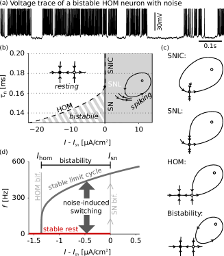
Figure 1: Bistability in homoclinic neurons. (a) Voltage trace of a homoclinic neuron (model definition in Sec. A, with gating time constant of $\tau_{n}=0.16\mathrm{ms}$) driven with $I=4.4\mu\mathrm{A/cm}^{2}$ and a noise strength of $\sigma=24\mathrm{mV}/\sqrt{\mathrm{s}}$ ($\frac{\sigma^{2}}{2}$ is the voltage diffusion constant in millivolt per second). (b) The homoclinic regime is reached by decreasing the time scale of the gating variable, $\tau_{n}$. Going from the SNIC to the homoclinic regime, the neuron passes the codimension-two SNL bifurcation, which is common to all class-1 excitable neurons. The SNL bifurcation thus acts as a gate to the bistable, homoclinic spiking regime (shaded area). (c) Phase plots (gating variable versus voltage) of neurons in different dynamical regimes, see panel 1(b) for parameter-space organization. (d) Horizontal transversal of the bifurcation diagram in 1(b) below the SNL point. Bistability of rest and spiking leads to hysteresis in the frequency-input curve of homoclinic neurons. Within the bistable region, noise can switch between rest and spiking.

The bistability of HOM neurons leads to a hysteresis in the firing-rate versus input curve, see Fig. 1(d): Ramping up the input current, $I$, the neuron stays at rest until the resting state loses stability at ${I_{\mathrm{sn}}}$. Conversely, when ramping down the input current, the neuron remains spiking until the limit cycle (LC) disappears at ${I_{\mathrm{hom}}}$. The region of bistability extends from ${I_{\mathrm{hom}}}$ to ${I_{\mathrm{sn}}}$. Consequently, noise-free deterministic neurons are easily probed experimentally for hysteresis effects by ramp currents which may then serve as an indicator for bistable membrane states. In experiments, many biological neuron types, however, may evade this kind of screening due to their high degree of stochasticity, in particular when their intrinsic noise causes them to constantly jump between attraction domains, resulting in a “mixed state” that is insensitive to the direction of parameter change. Yet, the change in interspike interval statistics and the switching probability between the two attractors that is derived in this article can still provide insight into the presence of bistability. As both measures can be estimated from recordings of biological neurons, they can be used to differentiate neurons in which the irregularity is solely due to noise from those in which the irregularity is enhanced by a bistability of the intrinsic dynamics. This might be particularly interesting when relating single-cell dynamics to the up- and downstates observed at network level. Previously, up- and downstates on the single-cell level are modeled by a bistability of two fixed points in the membrane voltage  [15–18]. The here considered setting is different, with a bistability between a fixed point of the membrane voltage (the resting state), and the limit cycle (spiking dynamics), yet if the upstate shows fast spiking behaviour this would be difficult to distinguish from the two-fixpoints case.

In the space spanned by the three fundamental parameters of conductance-based neuron models (i.e., membrane leak, capacitance and input current), a 2D-manifold of HOM bifurcations unfolds from the degenerate Bogdanov-Takens cusp point, which was proven to generically occur in these models  [19]. Starting with a model showing the common saddle-node on invariant cycle (SNIC) bifurcation at the creation of the spiking limit cycle, a decrease of the separation of timescales between voltage and gating kinetics switches the limit cycle creation to a HOM bifurcation along with the emergence of a bistability  [12], see Fig. 1(b). The switch in the bifurcation that creates the spiking limit cycle happens at the codimension-two saddle-node loop (SNL) bifurcation. It can be induced by many fundamental parameters in neuronal systems ranging from leak conductance, capacitance and temperature changes, to modifications of extracellular potassium concentration  [11]. Most importantly for the present article, between the HOM and the SN branch emerging from the SNL bifurcation there exists a region of bistable. Besides HOM neurons, bistability between rest and spiking also occurs in neuron models that undergo a subcritical Hopf bifurcation, followed by a fold of limit cycles at their firing onset. The spike statistics of these neuron models has previously been explored numerically  [25,26]. The spike statistics for SNIC neurons (upper part of the bifurcation diagram in Fig. 1(b)) is well characterised both for the excitable dynamics, i.e., $I<{I_{\mathrm{sn}}}$ (fluctuation driven  [10]), and the limit cycle dynamics, where $I>{I_{\mathrm{sn}}}$ (mean driven  [27]). The statistics in the bistable region of HOM neurons, however, is less studied and will be explored in this study. The derivation of the associated interspike interval statistics fills a gap of knowledge and provides the means to differentiate alternative underlying bifurcation structures using spike statistics. In particular, the following analysis focuses on the situation where the perturbing noise is weak such that the time evolution is still dominated by the attractors of the nonlinear dynamical system, with noise only switching between them.

Sec. II introduces the model for which in Sec. III the interspike interval density is derived. To this end, the stochastic trajectories are projected onto the unstable manifold of the saddle, see Sec. III.1. In this coordinate system both the statistics of intermittent silence, burst-firing and switching between these regimes are calculated in Sec. III.5, III.4 and III.2, respectively. Estimation of the probability of switching is discussed and the relation to ISI moments are presented in Sec IV. A comparison to a second kind of bistability is drawn in Sec. V.2 and the emergence of multimodal ISI densities as a meens of distinguising between them is addressed, see Sec. V.

II Conductance-based neuron model with homoclinic bistability

In the bistable regime, transitions between two stable attractors can be induced by noise fluctuations. The associated transition probability between the two attractors as well as the resulting spike statistics is derived in the following for a generic class of conductance-based neuron models with additive white noise and the limit cycle spike emerging from a HOM bifurcation. The analysis focuses on HOM neurons that are close to the SNL bifurcation, which allows for useful assumptions as introduced later.

The present analysis considers an $n$-dimensional conductance-based neuron model with one voltage dimension, the membrane voltage $v$, and a set of $n-1$ ion channel gates $a_{i}$. The dynamics of the state vector $\bm{x}=[v,a_{1},...,a_{n-1}]^{\top}\in{I\!\!R}^{n}$ is given by

$$\dot{\bm{x}}=\bm{F}(\bm{x})+\bm{D}(\bm{x})\bm{\xi}(t).$$ (1)

The additive noise $\bm{D}(\bm{x})\bm{\xi}$ originates from a diffusion approximation of either synaptic or intrinsic noise sources. The voltage dynamics follows a current-balance equation $F_{1}(\bm{x})=(I-I_{\mathrm{ion}}(\bm{x}))/{C_{\mathrm{m}}}$, with membrane capacitance ${C_{\mathrm{m}}}$, and the gates have first order kinetics, see also Appendix, Sec. A for model details. Details on the simulations are also stated in Appendix, Sec. A.

The analysis assumes that the model shows a HOM bifurcation from which the limit cycle spike emerges. A large class of conductance-based neuron models can be tuned into this regime  [11]. In HOM neurons, the limit cycle (corresponding to tonic firing) arises at $I={I_{\mathrm{hom}}}$ from a homoclinic orbit to the saddle, and at $I={I_{\mathrm{sn}}}>{I_{\mathrm{hom}}}$, saddle and stable node (corresponding to the neuron’s resting state) collide in a saddle-node bifurcation. For inputs in between, with ${I_{\mathrm{hom}}}<I<{I_{\mathrm{sn}}}$, the stable node and the limit cycle coexist as two stable attractors, see Fig. 1. The state space is divided into the basins of attraction of the fixpoint and the limit cycle by a separatrix (Fig. 2).

The analysis furthermore assumes that the noise strength is chosen small enough such that the spike shape is in first order not affected (the typical small noise approximation). With this, jumping between spiking and resting state is only possible close to the separatrix. While the separatrix is non-local, the following analysis shows that salient properties of its stochastic transition are given by the linearised dynamics around saddle and stable node.

The linearised dynamics around fixpoints are given by the Jacobian of Eq. 1, $J(\bm{x})=\frac{\partial\bm{F}(\bm{x})}{\partial\bm{x}}$, which has $n$ eigenvalues $\lambda_{1},...,\lambda_{n}$. For neuronal models undergoing a HOM onset bifurcation, the Jacobian at the saddle has one simple, positive, real eigenvalue corresponding to the unstable direction, denoted by $\lambda_{1}\in{I\!\!R}$. The other eigenvalues correspond to stable directions, such that

$$\lambda_{1}>0>\lambda_{2}\geqslant...\geqslant\lambda_{n}.$$ (2)

The associated orthonormal left and right eigenvectors are denoted by $\bm{l}_{k}$ and $\bm{r}_{k}$, $k\in[1,...,n]$, respectively, with $\bm{l}_{j}\cdot\bm{r}_{k}=\delta_{jk}$, see Fig. 3(a). Analytical expressions of $\bm{l}_{1}$ and $\bm{r}_{1}$ are given in the Appendix, in Sec. B for the saddle-node fixpoint, and in Sec. C for the saddle fixpoint.

The statistical properties of the bistable dynamical regime are not yet sufficiently characterised and will be explored in subsequent sections.

III Interspike interval

The following analysis considers the spike train of a HOM neuron in the bistable region, with ${I_{\mathrm{hom}}}<I<{I_{\mathrm{sn}}}$, subjected to white noise sufficiently strong to induce jumps between the two basins of attraction, e.g., Fig. 1(a). Between two consecutive spikes, the dynamics can either remain in the basin of attraction of the limit cycle, or it can visit the basin of attraction of the fixpoint before eventually returning to the limit cycle. On average, visiting the fixpoint will induce longer interspike intervals, because the escape from the resting state requires time in addition to the duration of the limit cycle.

Because the driving stochastic process is white, the process of subsequently occurring interspike intervals is renewal, as will be argued in Sec. III.2. The total interspike interval density is then a mixture of trajectories that remain on the limit cycle, and such trajectories with intermittent visits to the fixpoint. The interspike interval density of these two possibilities are denoted as

(i) the probability $p_{\mathrm{lc}}(t)$ that an interspike interval results from a trajectory staying exclusively on the limit cycle dynamics, and

(ii) the probability $p_{\mathrm{fp}}(t)$ that an interspike interval is composed of some time spent near the resting state in addition to the time required for the limit cycle spike following the escape of the fixpoint.

The total interspike interval density is a mixture of both kinds of trajectories,

$$p_{\mathrm{isi}}(t)=(1-{\varpi})\,p_{\mathrm{lc}}(t)+{\varpi}\,p_{\mathrm{fp}}(t),$$ (3)

where the factor $1-{\varpi}$ determines the proportion of intervals for which the dynamics resides entirely on the limit cycle side of the separatrix, while ${\varpi}$ is the proportion of intervals that include time spend on the fixpoint side of the separatrix.

In the following, ${\varpi}$ is called the mixing factor or splitting probability. For increasing values of ${\varpi}$, visits to the fixpoint become more frequent. In spike trains, this is visible as a larger proportion of long interspike intervals. The phenomemon of neurons showing strong ISI variability, with a ratio of long vs. short interspike intervals, is sometimes termed stochastic bursting, stuttering, irregularly spiking, or missing spikes in the experimental literature  [2,4,5].

In the following, the “ingredients” to approximate the interspike interval density in Eq. 3 are provided. The mixing factor ${\varpi}$ is derived in Sec. III.2, and the probabilities $p_{\mathrm{lc}}(t)$ and $p_{\mathrm{fp}}(t)$ in Secs. III.4 and III.5, respectively. To this aim, the system is transformed into a coordinate system that facilitates the analysis (Sec. III.1).

III.1 Projecting crossings of the separatrix on a double-well problem

The observation that most crossings of the separatrix happen along the downstroke of the action potential (AP) permits in the following to project the crossings of the separatrix onto a one-dimensional problem. More specifically, the high-dimensional problem of stochastic transitions through the $(n-1)$-dimensional separatrix is reduced to a one-dimensional double-well escape problem of which the occupancy statistics are known  [28].

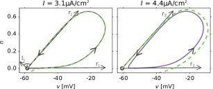
Figure 2: Depicted are left and right eigenvector of the saddle as well as the limit cycle (solid line) and the separatrix (dashed line). (a) At the HOM bifurcation, the homoclinic orbit overlaps with the separatrix. (b) For higher input amplitudes, the separatrix is shifted away from the limit cycle.

The separatrix between rest and spiking corresponds to the stable manifold of the saddle fixpoint. At the saddle, the tangent space of the separatrix is

$$\mathcal{T}=\Big{\{}\sum\nolimits_{k=2}^{n}\alpha_{k}\bm{r}_{k}:\alpha_{k}\in{I\!\!R}\Big{\}}.$$ (4)

The orthogonal complement is given by the left eigenvector $\bm{l}_{1}\in\mathcal{T}^{\perp}$, see Fig. 3(a) for a two-dimensional example.

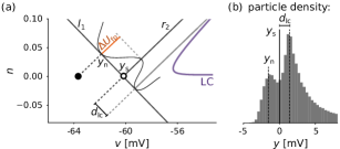
Figure 3: Equivalent double-well potential. (a) At the saddle ($\circ$), $\bm{r}_{2}$ is tangent to the stable manifold. Its orthogonal complement is $\bm{l}_{1}$, onto which the node ($\bullet$) and the minimum distance of the limit cycle ($d_{\mathrm{lc}}$) is projected. (b) Simulated particle density in the projected coordinate $y$.

For spike onset at $I={I_{\mathrm{hom}}}$, the separatrix overlaps with the homoclinic orbit, as both align per definition with the stable manifold of the saddle. For $I>{I_{\mathrm{hom}}}$, the limit cycle detaches from the saddle. The separatrix follows the limit cycle, until it eventually diverges, see Fig. 2. Along the spike downstroke, both the limit cycle and the separatrix remain parallel to the tangent space $\mathcal{T}$ for a significant part of the loop, for details see Appendix, Sec. E. Most relevant crossings of the separatrix happen in this region of the state space because

(i) due to the slow dynamics in the state space around the saddle, the limit cycle trajectory spends most of the time close to the saddle fixpoint, and

(ii) the distance between limit cycle and separatrix is minimal along the spike downstroke, allowing even weak noise deviations to switch the dynamics between rest and spiking.

In principle, multiple crossings back and forth across the separatrix are possible, but the final decision is taken when closing in on the saddle. In the vicinity of the saddle, trajectories on the limit cycle side of the tangent space $\mathcal{T}$ will follow limit cycle dynamics, while trajectories on the other side of the tangent space $\mathcal{T}$ will visit the stable fixpoint. The decision on which side of the separatrix a sample path is at a particular time can thus be read from a projection onto $\bm{l}_{1}\in\mathcal{T}^{\perp}$,

$$y(t)=\bm{l}_{1}\cdot(\bm{x}(t)-{\bm{x}_{\mathrm{s}}}),$$ (5)

where, for simplicity, the dynamics is recentred to the saddle at ${\bm{x}_{\mathrm{s}}}$, such that the saddle is in the projected coordinates located at ${y_{\mathrm{s}}}=0$. The position of the stable node is ${y_{\mathrm{n}}}=\bm{l}_{1}\cdot(\bm{x}_{\mathrm{n}}-{\bm{x}_{\mathrm{s}}})$, see Fig. 3(a). In the following, the convention is used that $y>0$ corresponds to the limit cycle side, while $y<0$ implies the fixpoint side, corresponding to the rest.

The following analysis uses the minimum distance of the deterministic limit cycle dynamics to the separatrix,

$$d_{\mathrm{lc}}=\mathop{\mathrm{argmin}}_{\bm{x}\in\Gamma}\{\bm{l}_{1}\cdot(\bm{x}-{\bm{x}_{\mathrm{s}}})\},$$ (6)

see Fig. 3(a). Here $\Gamma$ denotes the invariant set of the limit cycle. As mentioned above, the minimal distance is typically reached during the downstroke of the action potential. $d_{\mathrm{lc}}$ is the distance in the $\bm{l}_{1}$-direction of the projection along $\mathcal{T}$ of the closest point of the limit cycle to the separatrix.

The projection aims to collapse the decision, whether or not the fixpoint is visited, into one dimension such that the theory of double-well potentials can be applied to calculate the occupancy statistics. A histogram of the projected values, $y(t)$, from a simulation shows a bimodal density in Fig. 3(b). Such bimodal density also appear in the Brownian motion of a particle in a double-well potential. This motivates the here presented approach to reduce the properties of stochastic bursting in a high-dimensional neuron model to a double-well problem:

$$\dot{y}=-U^{\prime}(y)+\sigma\,\xi(t).$$ (7)

$y(t)$ here results from the projection of the dynamics onto the normal direction to the separatrix, as introduced above.

Approximations for the potential $U(y)$ and the noise strength $\sigma$ will be discussed for the different quantities that are calculated in the following sections.

III.2 Splitting probability

For uncorrelated noise, the series of spike-time events is a renewal process. After each spike, during the downstroke when the trajectory is close to the separatrix, the noise in the system operates akin to a (biased) coin flip that determines if the fixpoint is visited, or if immediately another round trip on the limit cycle is taken. Hence, the consecutive decisions from which distribution the spike times are drawn, i.e., $p_{\mathrm{lc}}(t)$ or $p_{\mathrm{fp}}(t)$, are Bernoulli trials (leading to a geometric distribution for the number of spikes per burst, see Eq. 21). Indeed, the statistics is reduced to calculating a single parameter: the splitting probability (or mixing factor) in a double-well potential.

The splitting probability in a double-well potential describes the probability of a particle that starts at a position in relation to the barrier to end up in one of the attractors first. In the present case the particle is initially injected $d_{\mathrm{lc}}$ away from the separatrix, see Fig. 3(a). The probabilty of crossing the barrier and reaching the fixpoint is denoted as $\varpi$. This probability can be found by solving the backward Fokker-Planck with the appropriate boundary conditions  [28]. The solution can be expressed in terms of the steady state density $p_{\mathrm{s}}(y)$ as

$$\varpi(d_{\mathrm{lc}})=\frac{\int_{d_{\mathrm{lc}}}^{\infty}p_{s}^{-1}(y)\mathrm{d}y}{\int_{y_{\mathrm{fp}}}^{\infty}p_{s}^{-1}(y)\mathrm{d}y}.$$ (8)

Here, the splitting probability depends on the distance between limit cycle and separatrix, $d_{\mathrm{lc}}$, which will be related to the system parameters in Sec. III.3.

The Fokker-Planck equation for the stochastic dynamics of the one dimensional projected variable $y(t)$ can always be written in potential form corresponding to Eq. 7

$$\partial_{t}p(y,t)=\partial_{y}\left[U^{\prime}(y)p(y,t)\right]+\frac{\sigma^{2}}{2}\partial_{y}^{2}p(y,t).$$

The stationary solution $p_{\mathrm{s}}$ to this equation can then be expressed in terms of the potential $U(y)$ as

$$p_{\mathrm{s}}(y)=\mathcal{N}\exp\Big{(}\frac{-U(y)}{2\sigma^{2}}\Big{)}.$$

Assume that the injection point is not to far from the separatrix which is at $y_{\mathrm{s}}=0$, and that the potential is sufficiently symmetric around the separatrix. The latter assumption is correct in the vicinity of the saddle-node bifurcation present in the neuron models considered here. When $U(y)$ is smooth, it is possible to assume that for small $d_{\mathrm{lc}}$,

$$U(y)\approx U(0)+\frac{1}{2}U^{\prime\prime}(0)d_{\mathrm{lc}}^{2}$$ (9)

Assuming $\sigma$ is small, the limit at $y=y_{fp}$ tends to $-\infty$. With Eq. 9, Eq. 8 changes into an expression involving Gaussian integrals. During the downstroke, the projected limit cycle dynamics near the separatrix is approximated by Eq. 7, where the potential in the direction of $\bm{l}_{1}$ is $U(y)=-\frac{\lambda_{1}}{2}y^{2}$, such that $U^{\prime\prime}(0)=-\lambda_{1}$. The “mixing noise” in that dimension is approximated by $\sigma^{2}=\sigma_{\mathrm{m}}^{2}=\bm{l}_{1}\cdot{\bm{D}}_{\mathrm{s}}\bm{l}_{1}$, with the diffusion matrix evaluated at the saddle, ${\bm{D}}_{\mathrm{s}}={\bm{D}}(\bm{x}_{\mathrm{s}})$. Together this yields

$$\varpi=\frac{1}{2}\bigg{(}1-\mathop{\mathrm{erf}}\Big{(}\frac{d_{\mathrm{lc}}\sqrt{\lambda_{1}}}{2\sigma_{\mathrm{m}}}\Big{)}\bigg{)}.$$ (10)

Here, $\mathop{\mathrm{erf}}(\cdot)$ denotes the error function. If the injection occurs at the separatrix, which corresponds to the situation when the spiking limit cycle is born from the homoclinic orbit (Fig. 2), the probability of ending up on either side of the separatrix is $1/2$. For increasing distance, the probability of visiting the fixpoint decays, see inset in Fig. 4(a), such that repetitive, burst-like, limit cycle excursions become more likely.

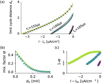
Figure 4: Comparison of theoretical prediction (lines) and numerical simulations (markers) for different gating time constants $\tau_{\mathrm{n}}$=0.155, 0.16 and 0.165ms. (a) Distance between limit cycle and separatrix, $d_{\mathrm{lc}}$, versus input current as given by Eq. 11. (b) Mixing factor ${\varpi}$ as a function of $d_{\mathrm{lc}}$. (c) $1-{\varpi}$ versus input current.

III.3 Limit cycle distance to the separatrix

The limit cycle originates from a homoclinic orbit at $I={I_{\mathrm{hom}}}$. As can be seen from the quadratic dynamics in the centre manifold of the saddle-node, the saddle, and thus the separatrix, moves as a square-root function of the input current. The limit cycle position is more invariant, see Appendix, Sec. D. Using Eq. 6, the distance of the limit cycle to the saddle in the centre manifold, and thus to the separatrix, is

$$d_{\mathrm{lc}}=\sqrt{\frac{l_{11}}{a\,{C_{\mathrm{m}}}}}(\sqrt{{I_{\mathrm{sn}}}-{I_{\mathrm{hom}}}}-\sqrt{{I_{\mathrm{sn}}}-I}),$$ (11)

where $l_{11}$ is the entry of the left eigenvector $\bm{l}_{1}$ that corresponds to the voltage dimension  [29]. The factor $a$ is the curvature term of the nullclines, and can be determined by  [30,31]

$$a=\frac{1}{2}\cdot\bm{l}_{1}\bm{H}\bm{r}_{1}\bm{r}_{1},$$ (12)

where $\bm{H}$ is the Hessian matrix of the deterministic dynamics.

Fig. 4(a) depicts the analytical $d_{\mathrm{lc}}$ from Eq. 11 and the simulated distance of the limit cycle to the separatrix as a function of the input current. For values of $I$ away from the saddle-node, ${I_{\mathrm{hom}}}<I\ll{I_{\mathrm{sn}}}$, the relation is rather linear. Hence, near the onset of bistability, the limit cycle distance can be approximated by

$$d_{\mathrm{lc}}\approx\sqrt{\frac{l_{11}}{2a\,{C_{\mathrm{m}}}}}\frac{I-{I_{\mathrm{hom}}}}{\sqrt{{I_{\mathrm{sn}}}-{I_{\mathrm{hom}}}}}.$$ (13)

With these expressions for the distance $d_{\mathrm{lc}}$, the mixing factor ${\varpi}$ can be calculated according to Eq. 10. For comparison, the mixing factor ${\varpi}$ is evaluated in stochastic simulations. To this end, the relative time spend on the side of the stable fixpoint and of the limit cycle is detected by recording a spike when a voltage threshold of -10mV is crossed from below; and recording a visit to the fixpoint when a two-dimensional threshold is crossed (crossing the voltage value of the saddle from above and the value of the $n$-variable 5% above the value corresponding to the node). The comparison between simulations and the analytical results can be inspected in Fig. 4(b).

Next, the probability $p_{\mathrm{lc}}(t)$ for staying on the limit cycle, the probability $p_{\mathrm{fp}}(t)$ for visiting the stable fixpoint, as well as the intra- and interburst statistics are calculated.

III.4 Intraburst statistics

This section determines the probability $p_{\mathrm{lc}}(t)$ for staying on the limit cycle without visiting the fixpoint used in Eq. 3. From this, the statistics of spikes inside a “burst” is derived, i.e., a consecutive sequence of limit cycle excursions uninterrupted by a crossing of the separatrix into the attraction domain of the fixpoint.

For trajectories that stay within the basin of attraction of the limit cycle and a sufficiently small noise amplitude, a phase reduction maps the process to a one-dimensional Brownian motion in the phase, $\theta$, which has constant drift,

$$\dot{\theta}=1/\tau_{\mathrm{lc}}+\sqrt{2\bar{D}_{\mathrm{lc}}}\,\xi(t).$$ (14)

Here, $\tau_{\mathrm{lc}}$ is the intrinsic, deterministic period of the limit cycle and $\xi(t)$ a stochastic white-noise process with effective diffusion matrix $\bar{D}_{\mathrm{lc}}$. The effective diffusion matrix, $\bar{D}_{\mathrm{lc}}$, is obtained by averaging the potentially non-stationary noise over the time scale of one interspike interval with an appropriate weighting function, $\bm{Z}_{1}$, that quantifies how susceptible the spike time is to perturbations at a given phase $\varphi$  [32]:

$$\bar{D}_{\mathrm{lc}}=\int_{0}^{1}d\varphi\,\bm{Z}_{1}(\varphi)\cdot\bm{D}(\bm{x}_{\mathrm{lc}}(\varphi))\bm{Z}_{1}(\varphi).$$ (15)

The weighting function is the so-called phase-response curve, $\bm{Z}_{1}(\theta)=\bm{\nabla}\theta\big{|}_{\bm{x}(\theta)=\bm{x}_{\mathrm{lc}}(\theta)}$, which can be determined numerically or calculated via centre manifold reductions  [31]. Provided that channel or synaptic fluctuations act on time scales faster than the average limit cycle period, the effective phase diffusion, $\bar{D}_{\mathrm{lc}}$, quantifies the averaged noise per interspike interval that causes jitter in the timing of spikes. It disregards radial excursions due to noise, in particular those that would cause jumps over the separatrix into the phaseless set (where no phase is defined). Assuming the intraburst dynamics is governed by the stochastic phase evolution in Eq. 14, the waiting-time density follows an inverse Gaussian distribution  [27,33]

$$p_{\mathrm{lc}}(t)=\frac{\exp\big{(}-\frac{(t-\tau_{\mathrm{lc}})^{2}}{\tau_{\mathrm{lc}}^{2}\,\bar{D}_{\mathrm{lc}}\,t}\big{)}}{\sqrt{\pi\,\bar{D}_{\mathrm{lc}}\,t^{3}}}.$$ (16)

The mean of the distribution, $\tau_{\mathrm{lc}}$, is identical to the deterministic period of the limit cycle. In the case of a homoclinic neuron, and close to the limit cycle onset (small $d_{\mathrm{lc}}$) it scales according to  [29]

$$\tau_{\mathrm{lc}}=-\frac{1}{\lambda}_{1}\ln(d_{\mathrm{lc}}).$$ (17)

Here, $d_{\mathrm{lc}}$ is again the distance of the limit cycle to the separatrix, cf. Eq. 6, which can be expressed in terms of system parameters in Eq. 11 and is required to fulfill $d_{\mathrm{lc}}\ll 1$.

III.5 Interburst statistics

This section develops the probability $p_{\mathrm{fp}}(t)$ for interspike intervals composed of a visit to the resting state fixpoint and a limit cycle spike used in Eq. 3. The interburst intervals resulting from fixpoint visits are on average longer than the intraburst intervals derived in the last section. The corresponding interspike interval, $t_{\mathrm{fp}}$, can be obtained by adding the time it takes for the trajectory to escape from the fixpoint, $t_{\mathrm{e}}$, and the proceeding time, $t_{\mathrm{lc}}$, for a spike excursion around the limit cycle, to obtain $t_{\mathrm{fp}}=t_{\mathrm{e}}+t_{\mathrm{lc}}$. The escape time, $t_{\mathrm{e}}$, from the resting state is described by Poisson statistics with a Kramer’s rate  [10]. The required assumption for Kramer’s theory, i.e., that the dynamics be equilibrated around the resting state, though not perfectly satisfied, appears reasonable enough, given that the decay time constant of the exponential decay is correctly described by the escape rate, as previously validated by comparisons with numerical simulations  [10]. However, there is disagreement in the very short ISIs  [10]. Therefore, in the present case, the escape rate is only supposed to describe the exit over the separatrix, which is then followed by the time taken for another limit cycle spike, $t_{\mathrm{lc}}$. If the escape and limit cycle dynamics were to be statistically independent, the waiting time of the complete interburst statistics $p_{\mathrm{fp}}(t)$ would be the convolution of the escape statistics $p_{\mathrm{e}}$ and the additional time corresponding to the duration of the spike, $p_{\mathrm{lc}}$, i.e.,

$$p_{\mathrm{fp}}(t)=(p_{\mathrm{lc}}*p_{\mathrm{e}})(t)=\int_{0}^{t}p_{\mathrm{lc}}(t-r)p_{\mathrm{e}}(r)\mathrm{d}r.$$ (18)

Note that Eq. 18 effectively describes a Poisson neuron with a refractory period drawn from $p_{\mathrm{lc}}$. The assumption of statistical independence can be motivated by two observations. Firstly, due to the fast contraction of the stable directions onto the one-dimensional unstable manifold at the saddle, the trajectories that leave the stable fixpoint are likely to penetrate the separatrix near one point. This gives delta-like initial condition for the limit cycle dynamics and to some extent clears the memory of the preceding trajectory. Secondly, the noise is uncorrelated.

The interval statistics of the escape, i.e., the Poisson neuron with Kramer’s rate $1/\tau_{\mathrm{e}}$, is exponential,

$$p_{\mathrm{e}}(t)=e^{-t/\tau_{\mathrm{e}}}/\tau_{\mathrm{e}}.$$ (19)

The mean interval $\tau_{\mathrm{e}}$ is given by the inverse of the Kramer’s rate  [10]

$$\tau_{\mathrm{e}}\approx\frac{2\pi}{|\lambda_{1}|}e^{\Delta{U_{\mathrm{sn}}}/2\sigma^{2}},$$ (20)

where $\lambda_{1}$ is the eigenvalue associated with the unstable manifold of the saddle. $\Delta{U_{\mathrm{sn}}}$ is the potential difference between saddle and node, $\Delta{U_{\mathrm{sn}}}={U_{\mathrm{sn}}}({y_{\mathrm{s}}})-{U_{\mathrm{sn}}}({y_{\mathrm{n}}})$. The latter can be approximated in the vicinity of the saddle-node bifurcation. Saddle and node depart from the saddle-node according to a square root function, such that locally ${y_{\mathrm{sn}}}=({y_{\mathrm{s}}}+{y_{\mathrm{n}}})/2$. If ${y_{\mathrm{s}}}$ and ${y_{\mathrm{n}}}$ have not departed too far from ${y_{\mathrm{sn}}}$, the potential $U$ is centrally symmetric around ${y_{\mathrm{sn}}}$ and hence has no quadratic part (i.e., the linear dynamics of saddle and node cancel in the middle). Therefore, the remaining dynamics can be captured in the following potential:

$${U_{\mathrm{sn}}}\approx\frac{({I_{\mathrm{sn}}}-I)(y-{y_{\mathrm{sn}}})}{{C_{\mathrm{m}}}}+\frac{a(y-{y_{\mathrm{sn}}})^{3}}{3},$$

with the factor $a$ from Eq. 26.

The potential difference between saddle and node is hence

$$\Delta{U_{\mathrm{sn}}}\approx(I-{I_{\mathrm{sn}}})({y_{\mathrm{n}}}-{y_{\mathrm{s}}})/{C_{\mathrm{m}}}+\frac{a}{12}({y_{\mathrm{n}}}-{y_{\mathrm{s}}})^{3}.$$

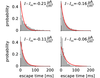
Figure 5: Near spike onset, the analytical escape rate (red) fits the probability density of the escape duration from fixpoint to the separatrix ($\tau_{\mathrm{n}}=0.165\mathrm{ms}$).

Using this approximation of the potential height in Eq. 20, the escape time density in Eq. 19 can be compared to the simulated neuron. The validity of the approximation can be inspected in Fig. 5 for different input currents. With this, all elements of the interspike density in Eq. 3 have been derived.

The full interspike interval distribution is plotted in Fig. 6 for one representative simulation, together with the analytical prediction.

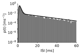
Figure 6: Interspike interval density for a numerical simulation with $\tau_{\mathrm{n}}=0.16\mathrm{ms}$, driven with $I=4.4\mu\mathrm{A/cm}^{2}$ plus current noise with $\sigma=0.8\sqrt{\mathrm{ms}}\mu\mathrm{A/cm}^{2}$. Mean ISI is 4.53 ms, coefficient of variation is 1.69.

III.6 Burst-length statistics and estimates of the splitting probability

As argued in Sec. III.2, the sequence of interspike intervals generated by the present bistable neuron, driven by white noise, is a renewal process, i.e., after each spike at the downstroke, the decision from which of the mixture components the interval is drawn happens irrespective of the previous intervals. Hence, no serial correlations between intervals are to be expected. Consequently, the burst length (number of consecutive limit cycle traverses before crossing the separatrix to the fixpoint) follows a geometric distribution which only depends on the splitting probability,

$$p(k)={\varpi}(1-{\varpi})^{k-1}.$$ (21)

Fig. 7 shows a comparison of numerically obtained burst-length statistics and the theory. This supports the initial assumption that the distribution of interspike intervals is indeed a renewal process. The discrepancy between simulations and theory observed for larger inputs results from the shape of the potential that separates stable fixpoint and limit cycle. For large inputs, the potential becomes shallow, such that repeated jumps over the separatrix become more likely. Even if the dynamics immediately jump back to the limit cycle, these events are in the simulations counted as fixpoint visits, while the theory only considers jumps that converge to the fixpoint. This leads to shorter bursts in the simulation compared to the theoretical expectations, as observed in Fig. 7 in the panel with $I-I_{\mathrm{sn}}=-0.06\mu A/cm^{2}$.

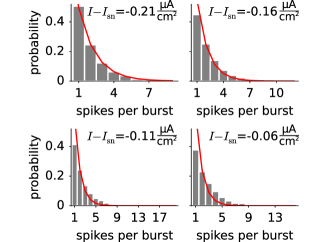
Figure 7: Burst-length statistics fitted using a geometric distribution and the splitting probability from Eq. 10.

If, for longer experimentally recorded spike trains, histograms of burst-length distribution are available, the splitting probability ${\varpi}$ can be inferred as the single parameter that fits $p(k)$ to the data.

IV Moments and parameter estimates

In the presence of noise, hysteresis effects as shown in Fig. 1, a distinctive signature of bistability in deterministic systems, may be obscured. But can bistability still be detected from stochastic properties of the spike time series? Once bistability is established, the previous section has identified multimodality as the distinguishing fact between the bistability resulting from a saddle-homoclinic orbit bifurcation versus a subcritical Hopf bifurcation.

The splitting probability, ${\varpi}$, may be taken as an indicator for which regime a neurons is driven,

1. ${\varpi}\approx 0\to$ mean-driven regime

2. ${\varpi}\approx 1\to$ fluctuation-driven regime

3. ${\varpi}\approx\frac{1}{2}\to$ bistable neuron

In Sec. III.6, it was surmised that for long enough spike trains, the mixing factor ${\varpi}$ could be estimated based on the burst-length statistics in Eq. 21. One may explore how the moments of the ISI distribution are related to system parameters. The uncentred moments of the ISI distribution are obtained from its Laplace transform in Eq. 22 via

$$\nu_{k}=(-1)^{k}\frac{\mathrm{d}^{k}}{\mathrm{d}s^{k}}P_{\mathrm{isi}}(s)\Big{|}_{s=0}.$$

Although the convolution in Eq. 18 cannot be evaluated analytically, its Laplace transform is a simple product of the transform of the inverse Gaussian distribution of the limit cycle dynamics,

$$P_{\mathrm{lc}}(s)=\exp\left(\left(1-\sqrt{1+2s\sigma_{\mathrm{lc}}^{2}\tau_{\mathrm{lc}}^{2}}\right)/\sigma_{\mathrm{lc}}^{2}\tau_{\mathrm{lc}}\right).$$

and that of the exponential distribution, which is $P_{\mathrm{fp}}=(1+s\tau_{\mathrm{e}})^{-1}$. Together the Laplace transform of the ISI distribution is

$$P_{\mathrm{isi}}(s)=(1-{\varpi})P_{\mathrm{lc}}(s)+\frac{{\varpi}P_{\mathrm{lc}}(s)}{1+s\tau_{\mathrm{e}}}.$$ (22)

Thus, mean and variance of $p_{\mathrm{isi}}(t)$ are given by

$$\mu_{\mathrm{isi}}={\varpi}\tau_{\mathrm{e}}+\tau_{\mathrm{lc}}$$ (23)

and

$$\sigma_{\mathrm{isi}}^{2}=(2-{\varpi}){\varpi}\tau_{\mathrm{e}}^{2}+\tau_{\mathrm{lc}}^{3}\sigma_{\mathrm{lc}}^{2}.$$ (24)

For the high firing rates present in HOM neurons with a small saddle-homoclinic orbit, the mean escape time $\tau_{\mathrm{e}}$ is the longest time scale in the system and can be estimated independently by fitting a histogram of the largest ISI samples. For low noise, $\tau_{\mathrm{lc}}$ can be estimated as the peak of the ISI histogram. Then, using Eq. 23, the mixing factor ${\varpi}$ can be estimated.

V Multimodal ISI densities in bistable neurons

Neuronal bistability at a separatrix connected to the stable manifold of a saddle is not the only known bistability in single neuron dynamics. Already in Hodgkin and Huxley’s equations for the squid axon a coexistence of resting and spiking was found for a small parameter range  [34]. In that case, for increasing input, a stable and an unstable limit cycle originate from a fold of limit cycle bifurcation and the unstable limit cycle subsequently terminates in a subcritical Hopf bifurcation, which also changes the stability of the fixpoint. ISI histograms estimated from numerical simulations of the squid model with noise  [25,26], as well as analytical calculations with simplified resonate-and-fire type models  [35,36], have suggested the presence of multimodal peaks in the ISI density. This raises the question if the kind of bistability in homoclinic neurons treated here can produce multimodal ISI densities, too, or if this hallmark can be used to differentiate between the two kinds of bistability?

V.1 HOM case

To answer the question of multimodality, the modes of the components of the mixture are examined. The inverse Gaussian, $p_{\mathrm{lc}}(t)$, has a single mode at

$$\hat{t}_{\mathrm{lc}}=\tau_{\mathrm{lc}}\left(\sqrt{1+\frac{9}{4}\tau_{\mathrm{lc}}^{2}\bar{D}_{\mathrm{lc}}^{2}}-\frac{3}{2}\tau_{\mathrm{lc}}\bar{D}_{\mathrm{lc}}\right).$$

The convolution with an exponential kernel does not produce additional peaks, and hence $p_{\mathrm{fp}}(t)$ as defined by the convolution in Eq. 18 is unimodal, too. The derivative of $p_{\mathrm{fp}}(t)$ is $\tau_{\mathrm{e}}p_{\mathrm{fp}}^{\prime}(t)=p_{\mathrm{lc}}(t)-p_{\mathrm{fp}}(t)$. If set to zero, it is found that it has a single mode $\hat{t}_{\mathrm{fp}}$ which satisfies

$$p_{\mathrm{lc}}(\hat{t}_{\mathrm{fp}})=p_{\mathrm{fp}}(\hat{t}_{\mathrm{fp}}),$$ (25)

i.e., the single mode is located at the crossing of the two distributions.

The curvature of $p_{\mathrm{fp}}$ is given by

$$p_{\mathrm{fp}}^{\prime\prime}(t)=\frac{1}{\tau_{\mathrm{e}}}(p_{\mathrm{lc}}^{\prime}(t)-p_{\mathrm{fp}}^{\prime}(t)).$$ (26)

The curvature at the mode is thus given by $p_{\mathrm{fp}}^{\prime\prime}(\hat{t}_{\mathrm{fp}})=p_{\mathrm{lc}}^{\prime}(\hat{t}_{\mathrm{fp}})/\tau_{\mathrm{e}}.$ The curvature is negative because $\hat{t}_{\mathrm{fp}}$ corresponds to a maximum. Hence, the mode of $p_{\mathrm{fp}}(t)$ is to be found on the declining part of $p_{\mathrm{lc}}(t)$, i.e., $\hat{t}_{\mathrm{lc}}<\hat{t}_{\mathrm{fp}}$.

The modes of the mixture distribution are confined to lie in the interval $[\hat{t}_{\mathrm{lc}},\hat{t}_{\mathrm{fp}}]$. Within this interval between both individual peaks, $p_{\mathrm{lc}}^{\prime}(t)<0$ and $p_{\mathrm{fp}}^{\prime}(t)>0$, such that Eq. 26 implies the concavity of $p_{\mathrm{fp}}(t)$. Let $\tilde{t}$ denote the inflection point of the declining part of the inverse Gaussian distribution, $p_{\mathrm{lc}}(t)$. The distribution $p_{\mathrm{lc}}(t)$ is concave on the interval $[\hat{t}_{\mathrm{lc}},\tilde{t}]$. Within the interval $[\hat{t}_{\mathrm{lc}},\min(\tilde{t},\hat{t}_{\mathrm{fp}})]$, both distributions, $p_{\mathrm{lc}}(t)$ and $p_{\mathrm{fp}}(t)$, are concave, which permits no more than a single peak for the mixing distribution. If the inflection point lies beyond the mode of $p_{\mathrm{fp}}(t)$, i.e., $\hat{t}_{\mathrm{fp}}<\tilde{t}$, this implies unimodality of $p_{\mathrm{isi}}(t)$. For the other case, $\hat{t}_{\mathrm{fp}}>\tilde{t}$, this implies no more than a peak on the interval $[\hat{t}_{\mathrm{lc}},\tilde{t}]$. For unimodality, it remains to be shown that the mixing distribution decays on the interval $[\tilde{t},\hat{t}_{\mathrm{fp}}]$. Within this interval, let us assume that $\tau_{\mathrm{e}}$ is the longest time scale in the system. According to Eq. 26, the density $p_{\mathrm{fp}}(t)$ can be made arbitrarily flat compared to the derivative $p_{\mathrm{lc}}^{\prime}(t)$ by increasing $\tau_{\mathrm{e}}$. This means that for sufficiently large $\tau_{\mathrm{e}}$, $p_{\mathrm{isi}}(t)$ is within the interval $[\tilde{t},\hat{t}_{\mathrm{fp}}]$ dominated by the derivative $p_{\mathrm{lc}}^{\prime}(t)$, and is thus negative with no possibility for a peak.

Coming back to the question of the modality of bistable homoclinic ISI density, it can be asserted that for large $\tau_{\mathrm{e}}$, which occur close to ${I_{\mathrm{hom}}}$, and with all other assumptions used in this article, the ISI density is unimodal. This is in contrast to at least a large proportion of bistable Hopf neurons and could offer a way to distinguish these regimes.

V.2 Subcritical Hopf case

The second type of bistability in conductance-based neuron models originates from the case where the stable limit cycle is born together with an unstable one out of a fold of limit cycles. The unstable limit cycle shrinks and may either be destroyed by a homoclinic bifurcation to a saddle  [11], or, as in the Hodgkin-Huxley equations in a subcritical Hopf bifurcation, which is the case discussed here and shown in Fig. 8b. The noise-driven dynamics of this latter case has been investigated in numerical simulations, where the ISI density was reported as multimodal  [25,26,37]. Furthermore, some geometric considerations about probable exit regions across the unstable limit cycle have been made  [37] and will be discussed in the following. While at present it is not fully understood how universal this multimodality is, it can be distinguished from the homoclinic case, which is not multimodal for sufficiently long escape times from the fixpoint as argued in Sec. V.1.

In the Hopf case, too, interspike intervals could be categorised into trajectories cycling around the stable limit cycle and those that visit the fixpoint region by crossing the circular separatrix given by the unstable limit cycle as shown in Fig. 8a. Within the basin of attraction of the stable focus, the dynamics can be linearised,

$$\dot{\bm{x}}=\bm{J}\bm{x}+\bm{B}\bm{\xi},$$ (27)

using the Jacobi matrix at the fixpoint, $\bm{J}$, and given the diffusion matrix, $\bm{D}=\frac{1}{2}\bm{B}\bm{B}^{\dagger}$. Assuming there is no focus-to-node transition in the region of bistability  [11], $\bm{J}$ has a pair of conjugate imaginary eigenvalues with negative real parts. In this case the dynamics shows noise-induced oscillation (alias quasicycles or subthreshold oscillations)  [38]. This class of noisy oscillations that do not require a deterministic limit cycle can still be described as phase oscillators using the recently found methods of backward and forward phases  [39,40]. Their average period is given by $\tau_{\mathrm{H}}=2\pi/\omega_{\mathrm{H}}$  [40], where $\omega_{\mathrm{H}}$ is the frequency given by the imaginary part of the Jacobian’s eigenvalues at the focus. What determines whether or not these quasi oscillations are reflected in the ISI density?

For random crossings of the separatrix, one might be inclined to think that the deterministic definition of phaseless sets  [41] implies that the phases of the spiralling dynamics inside the unstable orbit will not automatically carry to the phases of the stable limit cycle, defined by their isocrhons, and thus not influence spike timing histograms. A fortiori, since the isochrons of the stable limit cycle foliate around the unstable LC  [41,42] and thus, in a deterministic setting, all phases would be available for small perturbations crossing the separatrix and thus the subthreshold phase could be scrambled. Yet, the deterministic view is misleading as shown by numerous simulation studies reporting multimodality  [25,26]. Motivated in part by realistic noise sources such as ion channel fluctuations, previous considerations have focused on escape from the fixpoint which is restricted to a region on the unstable LC as a mechanism for multimodality and found additional peaks “in all ISI histograms [that] have been examined”  [37]. Indeed, the jump into the unstable limit cycle is typically confined to a region in state space, because action potentials with a required signal strength (AP height) need to have a resting state fixpoint that is in one corner of the AP limit cycle, away from the peak voltage. Due to the closeness of the AP trajectory and the unstable LC, transitions are likely to occur in this proximity, in particular if noise were to be restricted to the voltage dimension. The idea is that each time after completing another subthrehold cycle there is a probability of jumping out and initialising a spike at a narrow region in state space. It was previously concluded that “the second peak arises when the trajectory […] spirals round in the vicinity of the fixpoint for one cycle, and as the next cycle starts, it switches back to the stable limit cycle vicinity, thus creating an ISI roughly twice as long as the period of the stable limit cycle”  [37]. Actually, the quoted premise would not lead to a peak at double $\tau_{\mathrm{lc}}$ but with that reasoning the modes would be located at

$$\tau^{\mathrm{mode}}_{\mathrm{H}}=\tau_{\mathrm{lc}}+k\tau_{\mathrm{H}},\quad\text{for {\hbox{k=0,1,..}}.}$$

This predicted position of the secondary peaks in the ISI density is, however, still off as can be seen in Fig. 8c. A hint on why, may be inferred from the path simulation in Fig. 8a showing that as the unstable limit cycle is not very repellent, trajectories close to it will cycle around it for some time before switching to the large stable limit cycle of a spike at a specific region. In that case the mode should be found at multiples of the period of the unstable limit cycle, $\tau_{\mathrm{s}}$,

$$\tau^{\mathrm{mode}}_{\mathrm{s}}=\tau_{\mathrm{lc}}+k\tau_{\mathrm{s}},\quad\text{for {\hbox{k=0,1,..}},}$$

which fits better to the data.

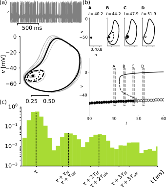
Figure 8: (a) Phase portrait and voltage trace of a stochastically bursting subcritical Hopf neuron are shown in grey. Stable and unstable limit cycle are shown as solid and dashed black line. Bistability region is found for DC input parameters between a fold of limit cycles and a subcritical Hopf bifurcation. The separatrix is an unstable limit cycle. (b) (A)-(D) show phase portraits before, after and during the emergence of the unstable limit cycle. Multimodal ISI histogram (c) for noise parameters derived from the analytically approximated unstable limit cycle in (a) and shown as the dotted ellipse in (a). Parameter of the neuron model can be found in  [29], Fig. 6.16.

In order to highlight that “regionalised exit”  [37] is not a prerequisite for multimodality in the ISI, the noise sources in the system were carefully tuned to render exit over the entire unstable limit cycle equally likely. Though this might be an unlikely scenario in a real nerve cell, it is a useful theoretical thought experiment to understand the requirements for multimodality. The scenario arises for small unstable limit cycles accompanied by a fortiori small noises with a special structure $\bm{D}$. The diffusion matrix has to be chosen such that the covariance matrix $\bm{\Sigma}$ of the stationary solution of Eq. 27 matches with the geometry of the surrounding unstable limit cycle. Close to the Hopf bifurcation the emerging unstable limit cycle can be approximated as an ellipse  [43]:

$$\Gamma(t)=\varepsilon(\bm{q}_{\Re}\cos(\omega_{\mathrm{H}}t)-\bm{q}_{\Im}\sin(\omega_{\mathrm{H}}t)),$$

where $\bm{q}_{\Re}$ and $\bm{q}_{\Im}$ are the real and imaginary part of the right eigenvector corresponding to the Hopf bifurcation. The covariance matrix $\bm{\Sigma}$ matches the geometry of the ellipse if $\bm{\Sigma}=\bm{q}_{\Re}\cdot\bm{q}_{\Re}^{\top}+\bm{q}_{\Im}\cdot\bm{q}_{\Im}^{\top}$. The diffusion matrix is then chose as  [28,40].

$$\bm{D}=-(\bm{J}\bm{\Sigma}+\bm{\Sigma}\bm{J}^{\top}).$$ (28)

With this choice of $\bm{D}$, exit though each segment of the unstable limit cycle is equiprobable.

The additional example of uniform exit highlights the fact that (i) the subthreshold backwards phase of the quasi cycles with associated period $\tau_{\mathrm{H}}$, (ii) the phase of the unstable limit cycle with associated period $\tau_{\mathrm{uLC}}$ and (iii) the phase associated with the stable limit cycle and isochrons and the period $\tau_{\mathrm{lc}}$ are all connected. This fact is different to to the saddle case where paths are contracted on the separatrix into almost a single point and hence the previous dynamics is not forgotten.

VI Discussion

Interspike-interval distributions are commonly investigated to characterise spiking behaviour in neurons. Experimentally, these distributions are easily measured by observing spike trains in response to step currents or noise injections. Theoretical distributions have been derived for several types of neuron models, in particular the Poissonian distribution for fluctuation-driven integrate-and-fire-type or conductance-based neuron models  [10], and the inverse Gaussian distribution for mean-driven neurons with a SNIC bifurcation at spike onset  [27,33,44]. Here, the interspike-interval distribution for neurons with a saddle-homoclinic orbit bifurcation, from which the limit cycle spike emerges, was derived within the bistable regime. These neurons show, close to spike onset, a region of bistability between resting state and spiking, and if the dynamics visits the resting state between two spikes, particularly long interspike intervals can ensue.

But can the present statistical analysis help to discern HOM/SNL, SNIC and Hopf bifurcations in recordings? Fitting inverse Gaussian, exponential or the bistable ISI density, as derived here, to recordings and comparing the model likelihood can be construed as supportive evidence for one or the other mechanism. However, for generalised inverse Gaussian distributions, it was shown that several diffusion processes can in principle result in the same waiting time distribution, or, conversely, ISI distributions cannot be uniquely mapped to their underlying diffusion processes  [45]. Therefore, caution is warranted not to overstress the generality of one’s inference about the mechanistic cause. Nonetheless, features of the ISI density, such as its skewness, have been related to underlying biophysical processes such as adaptation currents  [44,46]. A question similar in spirit may be whether neuronal bistability is uniquely tied to the ISI distribution derived in the present article?

In terms of the underlying bifurcation structure at least one other scenario giving rise to bistability of spiking and resting has been described previously and in Sec V.2: The subcritical Hopf bifurcation in association with a fold of limit cycles – present in the equations derived for the classical squid axon – also leads to a region of bistability and hysteresis  [34]. In combination with noise, numerical investigations  [25,26] indicated that the ISI distribution is multi-modal for the tested parameter combinations. At present, no parameters have been documented for which multimodality does not manifest in the ISI density. In the case of simplified resonate-and-fire models, the ISI distribution has been investigated analytically and multimodal peaks were confirmed  [35,36]. In contrast, the present manuscript argues for the absence of multimodality in the homoclinic-type bistability and hence this difference may be exploited to distinguish both kinds of bistability.

As was argued, bistability in homoclinic neurons can lead to spike time patterns, which resemble spiking observed experimentally in neurons, such as “stuttering cells”  [1,2] or “irregular spiking cells”  [3–5]. Some cells show membrane-voltage bistability in the form of distinct downstates and upstates  [47]. The likelihood of seeing this dynamics seems to be increased during sleep and certain anesthetics. The emergence of up-/downstates is associated with altered concentration dynamics in the intra- and extracellular space. Since the required time scale separation to induce the SNL bifurcation can also be achieved by modifying reversal potentials  [48], the resulting homoclinic bistability may be a putative, alternative mechanism underlying some of the up- and downstate dynamics observed in neurons. While up- and downstates have been modeled previously as bistable fixpoints in an integrate-and-fire like model  [14,18], the bistability between resting state and spiking dynamics introduced here is easily implemented in biologically more realistic conductance-based neuron model.

The emergence of bistability in neurons changes their coding properties, too. It has been noted that, in the absence of noise, rate coding in neurons close to a SNIC bifurcation is undermined by undesirable nonlinearities. More favorable for coding, bursting neurons have been shown to linearise the rate-tuning curve  [49]. Furthermore, in a network, bistability in the membrane voltage has been shown to increase the power for certain frequency bands of a population transfer function  [18]. In a similar way, the filtering associated with individual homoclinic neurons can transfer considerably higher frequencies during the spiking periods  [50]. Hence, spike-timing based codes can benefit from the high-frequency coding arising from the symmetry breaking that is induced by the switch in spike generation from SNIC to HOM at the SNL point  [12]. The option to visit the fixpoint before spiking adds to the versatile coding possibilities of these neurons when explicitly considering their bistability. An open question is if the interspike-interval distribution of the bistable neuron has favourable properties similar to the power-law interspike interval density appearing in some theories of optimal coding  [52]: The mutual information between a fast stimulus and the emitted spike train is bounded from above by the output entropy of the alphabet (i.e., the spike train entropy)  [53]. The spike train entropy is increased by more diverse spike patterns arising from the stochastic bursting responses in the bistable regime, compared to the tonic response of a SNIC neuron. It remains to be shown how the conditional entropy is influenced, which also contributes to the system’s information transmission rate.

Early theories of spiking network dynamics have, for simplicity, assumed identical neurons. Networks of such identical, yet highly stochastic, spiking neurons can generate global rhythms  [54]. Even with mild heterogeneity in the network delays, these phenomena seem to persist  [55]. Neuron-intrinsic heterogeneity has also been investigated in networks of leaky integrate-and-fire (IF) units, using randomly distributed thresholds. Under a rate coding regime an optimal level of heterogeneity was suggested  [56]. Yet, with leaky IF models lack the rich bifurcation structure of conductance-based models. Particularly, heterogeneity in thresholds will not produce the drastic and critical changes described in the present article. The impact of heterogeneity in single-neuron parameters that bring about SNL bifurcations in networks may be surmised to be substantial, but awaits further studies.

Integrate-and-fire models focus on capturing only the spike upstroke dynamics while relying on a reset for the spike downstroke. These models have been used to investigate the influence of rapid upstroke dynamics (in part influenced by Na⁺ channel dynamics) on coding  [57], and network dynamics  [58]. The quadratic IF model can be derived from the centre manifold reduction of saddle-node bifurcations  [30], and can with an appropriately chosen reset serve as the “normal form” of the bifurcation structure in Fig. 1(b)  [21,29]. Then again, this article shows the switching dynamics to occur outside the centre manifold dynamics during the downstroke along the strongly stable direction. Hence, the window of opportunity for jumping the separatrix is more related to the timescale of the K⁺ channel dynamics. Nonetheless, the quadratic IF with a reset above the unstable fixpoint and noise will produce the same ISI dynamics as derived here and can thus be taken as a simplified form in network theories of homoclinic bistable neurons.

In summary, the interspike interval distribution derived in this paper is useful on various levels. It provides an experimental check for bistability due to homoclinic spike generation, conveys information on coding properties, and forms the basis for a mean-field theory for networks with bistable single-neuron dynamics. Translated to other oscillating systems, the analysis might even inform about homoclinic bistability beyond the neurosciences.

VII Acknowledgments

Funded by the German Federal Ministry of Education and Research (No. 01GQ1403) and the Deutsche Forschungsgemeinschaft (No. GRK1589/2). Authors J.-H.S. and J.H. contributed equally to this work. The authors would like to thank Paul Pfeiffer for useful comments on the manuscript.

Appendix A Model definition

For illustrative purposes, a planar conductance-based neuron model is considered, but the analysis can be extend to $n$-dimensional models provided the stable manifold of the saddle is $n-1$ dimensional.

$${C_{\mathrm{m}}}\dot{v}=I-I_{\mathrm{ion}}$$

$$\tau_{\mathrm{n}}(v)\dot{n}=n_{\infty}(v)-n$$

$\tau_{\mathrm{n}}(v)$ is a bounded function of the voltage.

For numerical simulations, two-dimensional sodium-potassium neuron models are used  [29]. Model parameters for the neuron with a saddle-homoclinic orbit bifurcation are given in Table 1 and for the neuron with a subcritical Hopf bifurcation in Table 2. For both models, the ionic current is

$$I_{\mathrm{ion}}=g_{\mathrm{L}}(E_{\mathrm{L}}-v)+g_{\mathrm{Na}}m_{\infty}(v)(E_{\mathrm{Na}}-v)+g_{\mathrm{K}}n(E_{\mathrm{K}}-v).$$

The activation curves of the gates are

$m_{\infty}=\frac{1}{1+\exp(-\frac{v/\mathrm{mV}+25}{5})}$

$n_{\infty}=\frac{1}{1+\exp(-\frac{v/\mathrm{mV}+29}{15})}$

The gating time constant is independent of $v$, $\tau_{\mathrm{n}}(v)=\tau_{\mathrm{n}}$.

Table 1: Model parameters of the sodium-potassium neuron used for the simulations of the homoclinic neuron.

Parameter		Value
Membrane capacitance	$C_{\mathrm{m}}$	$1\mu$F/cm2
Leak reversal potential	$E_{\mathrm{L}}$	$-80$mV
Sodium reversal potential	$E_{\mathrm{Na}}$	$60$mV
Potassium reversal potential	$E_{\mathrm{K}}$	$-90$mV
Maximal leak conductance	$g_{\mathrm{L}}$	$8\mathrm{mS/cm}^{2}$
Maximal sodium cond.	$g_{\mathrm{Na}}$	$20\mathrm{mS/cm}^{2}$
Maximal potassium cond.	$g_{\mathrm{K}}$	$10\mathrm{mS/cm}^{2}$
Gating time constant	$\tau_{\mathrm{n}}$	$0.165\mathrm{ms}$

Table 2: Model parameters of the sodium-potassium neuron used for the simulations of the subcritical Hopf neuron.

Parameter		Value
Membrane capacitance	$C_{\mathrm{m}}$	$1\mu$F/cm2
Leak reversal potential	$E_{\mathrm{L}}$	$-78$mV
Sodium reversal potential	$E_{\mathrm{Na}}$	$60$mV
Potassium reversal potential	$E_{\mathrm{K}}$	$-90$mV
Maximal leak conductance	$g_{\mathrm{L}}$	$1\mathrm{mS/cm}^{2}$
Maximal sodium cond.	$g_{\mathrm{Na}}$	$4\mathrm{mS/cm}^{2}$
Maximal potassium cond.	$g_{\mathrm{K}}$	$4\mathrm{mS/cm}^{2}$
Gating time constant	$\tau_{\mathrm{n}}$	$1.0\mathrm{ms}$

Voltage dynamics were simulated in the simulation environment brian2 using the internal noise term xi  [59].

Appendix B Directions of stable and unstable manifold around the saddle-node

For the saddle-node, $\lambda_{1}=0$, and the associated right eigenvector is given by

1. $\bm{r}_{1}=\frac{1}{\kappa}\begin{pmatrix}1\\ \tau_{k}\frac{\partial F_{k}}{\partial v}\\ \vdots\end{pmatrix}=\frac{1}{\kappa}\begin{pmatrix}1\\ \frac{\mathrm{d}}{\mathrm{d}v}{a^{(\infty)}}_{k}(v)|_{v={v_{\mathrm{sn}}}}\\ \vdots\end{pmatrix}$,

where $v={v_{\mathrm{sn}}}$ and $a_{k}={a^{(\infty)}}_{k}(v)$ was used  [31]. The eigenvector $\bm{r}_{1}$ is tangential to the semi-stable manifold, which corresponds to the centre manifold of the SNIC bifurcation.

For the saddle-node, the right eigenvectors to $\lambda_{2},…,\lambda_{n}$ span the tangential space to the stable manifold. Due to the orthogonality of left and right eigenvectors, the normal to the tangent space of the stable manifold is given by the left eigenvector corresponding to the unstable direction, $\bm{l}_{1}$  [31],

1. $\bm{l}_{1}=\begin{pmatrix}1\\ \tau_{k}\frac{\partial F_{0}}{\partial a_{k}}\\ \vdots\end{pmatrix}.$

Appendix C Directions of stable and unstable manifold around the saddle

The analysis of the HOM neuron model assumes that the spike onset lies in proximity to the SNL bifurcation, such that the saddle at ${I_{\mathrm{hom}}}$ inherits properties of the saddle-node at ${I_{\mathrm{sn}}}$. It is shown in the following for a planar model that this implies similar linearised dynamics along the unstable manifold of saddle and saddle-node. To this aim, the eigenvectors around the saddle are expressed as the eigenvectors of the saddle-node, as given in Sec. B, plus a small term. The closeness of the saddle to the saddle-node is translated into two mathematical assumptions: It is assumed that $\lambda_{1}\ll 1$ at the saddle (because $\lambda_{1}=0$ at the saddle-node), and it is assumed that the voltage values of saddle and saddle-node are similar, $\Delta v=v_{\mathrm{saddle}}-v_{\mathrm{sn}}\ll 1$.

The linearised dynamics around saddle or saddle-node are given by their Jacobian. The Jacobian of a two-dimensional system akin to the model in Sec. A is given as

$\bm{J}=\begin{pmatrix}\frac{\partial F_{0}}{\partial v}&\frac{\partial F_{0}}{\partial n}\\ \frac{\partial F_{1}}{\partial v}&\frac{\partial F_{1}}{\partial n}\end{pmatrix}=\begin{pmatrix}a&b\\ c&d\end{pmatrix}$.

For a two-dimensional matrix, the eigenvalues are $\lambda_{1/2}=0.5(a+d\pm E)$ with $E=\sqrt{a^{2}-2ad+4bc+d^{2}}$. The right eigenvector corresponding to $\lambda_{1}$ is $r_{1}=(1,\frac{2c}{E+a-d})$, the left eigenvector is $l_{1}=(1,\frac{2b}{E+a-d})$ (equal to the right eigenvalue of the transposed matrix).

Expressing $E$ by $\lambda_{1}$ gives $r_{1}=(1,\frac{c}{-d+\lambda_{1}})$ and $l_{1}=(1,\frac{b}{-d+\lambda_{1}})$.

The assumptions allow to approximate the expressions for the eigenvectors. Because $d=-1/\tau_{n}(v)$ is a bounded function of the voltage, and because of the assumption $\lambda_{1}<<1$, one finds $\frac{b}{-d+\lambda_{1}}=\frac{b}{-d}\cdot\frac{1}{1+\frac{\lambda_{1}}{-d}}\approx\frac{b}{-d}\cdot(1-\frac{\lambda_{1}}{-d})$. Furthermore, the assumptions $\Delta v<<1$ allows one to develop $b(v)$ and $c(v)$ around $v_{\mathrm{sn}}$, with $v=v_{\mathrm{sn}}+\Delta v$.

$$\bm{r}_{1}\approx(1,\frac{\partial n_{\infty}}{\partial v})+(0,\tau_{n}\lambda_{1})$$

$$\approx(1,\frac{\partial n_{\infty}}{\partial v}(v_{\mathrm{sn}}))+(0,\frac{\partial^{2}n_{\infty}}{\partial v^{2}}(v_{\mathrm{sn}})\Delta v+\tau_{n}\lambda_{1}),$$

$$\bm{l}_{1}\approx(1,\tau_{n}\frac{\partial F_{0}}{\partial n})+(0,\tau_{n}\lambda_{1})$$

$$\approx(1,\tau_{n}\frac{\partial F_{0}}{\partial n}(v_{\mathrm{sn}}))+(0,-g_{\mathrm{k}}\,p\,n^{p-1}\Delta v+\tau_{n}\lambda_{1}),$$

where $b=g_{\mathrm{k}}\,n^{p}\,(E_{\mathrm{k}}-v)$ was used for $l_{1}$.

For $\lambda_{1}=0$, $\Delta v=0$, $\bm{r}_{1}$ and $\bm{l}_{1}$ at the saddle-node fixpoint (see Sec. B) are recovered. This shows that the linear dynamics at the saddle and at the saddle-node are similar for small $\lambda_{1}$ and $\Delta v$, in the sense that the linearised dynamics around the saddle-node are the zeroth order term of an expansion of the linearised dynamics around the saddle in $\lambda_{1}$ and $\Delta v$.

Appendix D Limit cycle downstroke is in first order independent of the input

The simulations in Fig. 9(a) show that the location of the limit cycle remains surprisingly constant with an increase in input current. This can be understood by observing that for the flow on the limit cycle, the major change in velocity occurs in proximity to the saddle: The flow on the limit cycle trajectory, $\Gamma$, is given by the velocity at each point $(v,n)\in\Gamma$. The speed of the gating, $\dot{n}$, is independent of ${I}$. The speed of the voltage, $\dot{v}=({I}+I_{\mathrm{ion}})/{C_{\mathrm{m}}}$, depends on ${I}$, but the influence of ${I}$ is small as long as ${I}<<I_{\mathrm{ion}}$. During the spike, ionic currents dominate the dynamics (Fig. 9(c)), and $I_{\mathrm{ion}}$ has the same order of magnitude as ${I}$ only in between two spikes, i.e., close to the saddle (green background in Fig. 9(c)). This implies that the only significant changes in the limit cycle trajectory happen close to the saddle, as suggested by the simulations of the limit cycle trajectory, see Fig. 9(a).

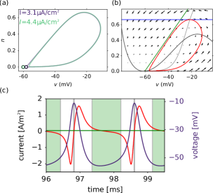
Figure 9: Location of the limit cycle. (a) For inputs above spike onset, the limit cycle position remains relatively stable, while saddle (open circle), and thus separatrix, move. (b) The downstroke of the limit cycle aligns with $\bm{r}_{2}$ (green line). Nullclines are shown for voltage (dark grey) and gating variable (light grey). (c) During the spike (violet voltage trace), the ionic current $I_{\mathrm{ion}}$ (red) is orders of magnitude larger than the input current ${I}$ (green horizontal line). Green background marks the area in which $I_{\mathrm{ion}}<10{I}$.

Appendix E At spike onset, the limit cycle downstroke aligns with the stable eigenvector of the saddle

The derivation in the main text assumes that the downstroke of the limit cycle follows the stable $\bm{r}_{2}$ eigenvector of the saddle at spike onset. This is trivially true for the saddle-homoclinic orbit in an infinitesimal small environment of the saddle. As shown in the following, this also holds for a significant part of the dynamics along the spike downstroke.

The argument relies on the following observations. For the homoclinic orbit attached to the saddle, two points in the phase plane are known. (1.) The downstroke of the homoclinic orbit attaches to the saddle. More precisely, it enters the saddle along its stable manifold tangential to $r_{2}$ (Fig. 9(b), green line). (2.) At the limit cycle maximum in the phase plane, $(v(n_{\mathrm{max}}),n_{\mathrm{max}})$ with $n_{\mathrm{max}}=\max_{t}(n_{\mathrm{LC}}(t))$, the flow is tangential to the voltage direction, i.e., $\dot{n}=0$, such that the maximum lies on the gating nullcline given by $n_{\infty}(v)$ (Fig. 9(b)). Because the limit cycle circles around the unstable node or focus, the limit cycle maximum $(v(n_{\mathrm{max}}),n_{\mathrm{max}})$ lies above the unstable node or focus. Because voltage and gating nullclines cross at the unstable node or focus, the limit cycle downstroke, once it has passed $(v(n_{\mathrm{max}}),n_{\mathrm{max}})$, lies above both nullcline. In consequence, the velocity along the downstroke trajectory points in the direction of the third quadrant (i.e., to the bottom left), such that the trajectory approaches $\bm{r}_{2}$ monotonously. As the trajectory of the limit cycle downstroke has a horizontal velocity at $(v(n_{\mathrm{max}}),n_{\mathrm{max}})$ and a velocity aligned to $r_{2}$ at the saddle, and approaches $r_{2}$ monotonically, the expectation of smooth trajectories allows to conclude that the trajectory of the saddle-homoclinic orbit aligns for a significant part of the limit cycle with $\bm{r}_{2}$.

References

[1] A. Gupta, Y. Wang, and H. Markram, Science 287, 273 (2000).

[2] C. Song, X.-B. Xu, Y. He, Z.-P. Liu, M. Wang, X. Zhang, B.-M. Li, and B.-X. Pan, PLoS ONE 8, (2013).

[3] M. Galarreta, F. Erdélyi, G. Szabó, and S. Hestrin, Journal of Neuroscience 24, 9770 (2004).

[4] K. M. Stiefel, B. Englitz, and T. J. Sejnowski, Proceedings of the National Academy of Sciences 110, 7886 (2013).

[5] P. R. Mendonça, M. Vargas-Caballero, F. Erdélyi, G. Szabó, O. Paulsen, and H. P. Robinson, eLife 5, (2016).

[6] E. Adrian, The Basis of Sensation: The Action of the Sense Organs (Christophers, 1928).

[7] S. Schreiber, I. Samengo, and A. V. M. Herz, Journal of Neurophysiology 101, 2239 (2008).

[8] M. Stemmler, Network: Computation in Neural Systems 7, 687 (1996).

[9] C. Ly and B. Doiron, PLoS ONE 12, (2017).

[10] C. C. Chow and J. A. White, Biophysical Journal 71, 3013 (1996).

[11] C. Kirst, J. Ammer, F. Felmy, A. Herz, and M. Stemmler, Fundamental Structure and Modulation of Neuronal Excitability: Synaptic Control of Coding, Resonance, and Network Synchronization (2015).

[12] J. Hesse, J.-H. Schleimer, and S. Schreiber, Physical Review E 95, (2017).

[13] A. L. Hodgkin, The Journal of Physiology 107, 165 (1948).

[14] S. G. Cogno, S. Schreiber, and I. Samengo, Neural Computation 26, 2798 (2014).

[15] C. J. Wilson and Y. Kawaguchi, The Journal of Neuroscience: The Official Journal of the Society for Neuroscience 16, 2397 (1996).

[16] R. H. Lee and C. J. Heckman, Journal of Neurophysiology 80, 583 (1998).

[17] S. R. Williams, S. R. Christensen, G. J. Stuart, and M. Häusser, The Journal of Physiology 539, 469 (2002).

[18] W. Wei, F. Wolf, and X.-J. Wang, Physical Review E 92, (2015).

[19] C. Kirst, Synchronization, Neuronal Excitability, and Information Flow in Networks of Neuronal Oscillators, PhD thesis, Niedersächsische Staats-und Universitätsbibliothek Göttingen, 2012.

[20] S. Schecter, SIAM Journal on Mathematical Analysis 18, 1142 (1987).

[21] S.-N. Chow and X.-B. Lin, Differential and Integral Equations 3, 435 (1990).

[22] P. Aguirre, SIAM Journal on Applied Dynamical Systems 14, 1600 (2015).

[23] A. J. Homburg and B. Sandstede, Journal (2003).

[24] J. Guckenheimer and J. S. Labouriau, Bulletin of Mathematical Biology 55, 937 (1993).

[25] H. C. Tuckwell and J. Jost, Physica A: Statistical Mechanics and Its Applications 391, 5311 (2012).

[26] P. F. Rowat and P. E. Greenwood, Frontiers in Computational Neuroscience 8, (2014).

[27] G. L. Gerstein and B. Mandelbrot, Biophysical Journal 4, 41 (1964).

[28] C. W. Gardiner, Handbook of Stochastic Methods for Physics, Chemistry, and the Natural Sciences, 3rd ed (Springer-Verlag, Berlin ; New York, 2004).

[29] E. M. Izhikevich, Dynamical Systems in Neuroscience (MIT Press, 2007).

[30] B. Ermentrout and N. Kopell, SIAM Journal on Applied Mathematics 46, 233 (1986).

[31] J.-H. Schleimer and S. Schreiber, Mathematical Methods in the Applied Sciences 41, 8844 (2018).

[32] J. H. Schleimer, Spike Statistics and Coding Properties of Phase Models, PhD thesis, Humboldt-Universität zu Berlin, Mathematisch-Naturwissenschaftliche Fakultät I, 2013.

[33] E. Schroedinger, Physikalische Zeitschrift 16, 289 (1915).

[34] M. E. Rush and D. J. Rinzel, Bulletin of Mathematical Biology 57, 899 (1995).

[35] T. Verechtchaguina, I. M. Sokolov, and L. Schimansky-Geier, Biosystems 89, 63 (2007).

[36] T. A. Engel, L. Schimansky-Geier, A. V. M. Herz, S. Schreiber, and I. Erchova, Journal of Neurophysiology 100, 1576 (2008).

[37] P. Rowat, Neural Computation 19, 1215 (2007).

[38] H. A. Brooks and P. C. Bressloff, Physical Review E 92, (2015).

[39] P. J. Thomas and B. Lindner, Physical Review Letters 113, (2014).

[40] P. J. Thomas and B. Lindner, Physical Review E 99, (2019).

[41] J. Guckenheimer, Journal of Mathematical Biology 1, 259 (1975).

[42] H. M. Osinga and J. Moehlis, SIAM Journal on Applied Dynamical Systems 9, 1201 (2010).

[43] Y. A. Kuznetsov, Elements of Applied Bifurcation Theory (Springer Science & Business Media, 2004).

[44] T. Schwalger, K. Fisch, J. Benda, and B. Lindner, PLoS Computational Biology 6, (2010).

[45] O. Barndorff-Nielsen, P. Blesild, and C. Halgreen, Stochastic Processes and Their Applications 7, 49 (1978).

[46] K. Fisch, T. Schwalger, B. Lindner, A. V. M. Herz, and J. Benda, Journal of Neuroscience 32, 17332 (2012).

[47] Y. Loewenstein, S. Mahon, P. Chadderton, K. Kitamura, H. Sompolinsky, Y. Yarom, and M. Häusser, Nature Neuroscience 8, 202 (2005).

[48] P. J. Hahn and D. M. Durand, Journal of Computational Neuroscience 11, 5 (2001).

[49] D. J. MacGregor and G. Leng, PLoS Computational Biology 8, (2012).

[50] E. Brown, J. Moehlis, and P. Holmes, Neural Computation 16, 673 (2004).

[51] J.-H. Schleimer and M. Stemmler, Physical Review Letters 103, 248105 (2009).

[52] Y. Tsubo, Y. Isomura, and T. Fukai, PLoS Computational Biology 8, (2012).

[53] S. P. Strong, R. Koberle, R. R. de Ruyter van Steveninck, and W. Bialek, Physical Review Letters 80, 197 (1998).

[54] N. Brunel and V. Hakim, Neural Computation 11, 1621 (1999).

[55] N. Brunel, Journal of Computational Neuroscience 8, 183 (2000).

[56] J. F. Mejias and A. Longtin, Physical Review Letters 108, (2012).

[57] N. Fourcaud-Trocmé, D. Hansel, C. van Vreeswijk, and N. Brunel, The Journal of Neuroscience 23, 11628 (2003).

[58] M. Monteforte and F. Wolf, Physical Review Letters 105, (2010).

[59] M. Stimberg, D. F. M. Goodman, V. Benichoux, and R. Brette, Frontiers in Neuroinformatics 8, (2014).