Superconvergence of $C^{0}-Q^{k}$ finite element method for elliptic equations with approximated coefficients

Abstract

We prove that the superconvergence of $C^{0}$-$Q^{k}$ finite element method at the Gauss Lobatto quadrature points still holds if variable coefficients in an elliptic problem are replaced by their piecewise $Q^{k}$ Lagrange interpolants at the Gauss Lobatto points in each rectangular cell. In particular, a fourth order finite difference type scheme can be constructed using $C^{0}$-$Q^{2}$ finite element method with $Q^{2}$ approximated coefficients.

65N30, 65N15, 65N06

1 Introduction

1.1 Motivations

Consider solving a variable coefficient Poisson equation

(1) $$-\nabla\cdot(a\nabla u)=f,\quad a(x,y)>0$$

with homogeneous Dirichlet boundary conditions on a rectangular domain $\Omega$. Assume that the coefficient $a(x,y)$ and the solution $u(x,y)$ are sufficiently smooth. Let $\|u\|_{k,p,\Omega}$ be the norm of Sobolev space $W^{k,p}(\Omega)$. For $p=2$, let $H^{k}(\Omega)=W^{k,2}(\Omega)$ and $\|\cdot\|_{k,\Omega}=\|\cdot\|_{k,2,\Omega}$. The subindex $\Omega$ will be omitted when there is no confusion, e.g., $\|u\|_{0}$ denotes the $L^{2}(\Omega)$-norm and $\|u\|_{1}$ denotes the $H^{1}(\Omega)$-norm. The variational form is to find $u\in H_{0}^{1}(\Omega)=\{v\in H^{1}(\Omega):v|_{\partial\Omega}=0\}$ satisfying

(2) $$A(u,v)=(f,v),\quad\forall v\in H_{0}^{1}(\Omega),$$

where $A(u,v)=\iint_{\Omega}a\nabla u\cdot\nabla vdxdy$, $(f,v)=\iint_{\Omega}fvdxdy.$ Consider a rectangular mesh with mesh size $h$. Let $V_{0}^{h}\subseteq H^{1}_{0}(\Omega)$ be the continuous finite element space consisting of piecewise $Q^{k}$ polynomials (i.e., tensor product of piecewise polynomials of degree $k$), then the $C^{0}$-$Q^{k}$ finite element solution of (2) is defined as $u_{h}\in V_{0}^{h}$ satisfying

(3) $$A(u_{h},v_{h})=(f,v_{h}),\quad\forall v_{h}\in V_{0}^{h}.$$

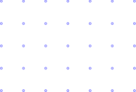
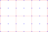
For implementing finite element method (3), either some quadrature is used or the coefficient $a(x,y)$ is approximated by polynomials for computing $\iint_{\Omega}au_{h}v_{h}\,dxdy$. In this paper, we consider the implementation to approximate the smooth coefficient $a(x,y)$ by its $Q^{k}$ Lagrangian interpolation polynomial in each cell. For instance, consider $Q^{2}$ element in two dimensions, tensor product of 3-point Lobatto quadrature form nine uniform points on each cell, see Figure 1. By point values of $a(x,y)$ at these nine points, we can obtain a $Q^{2}$ Lagrange interpolation polynomial on each cell. Let $a_{I}(x,y)$ and $f_{I}(x,y)$ denote the piecewise $Q^{k}$ interpolation of $a(x,y)$ and $f(x,y)$ respectively. For a smooth functions $a\geq C>0$, the interpolation error on each cell $e$ is $\max_{\mathbf{x}\in e}|a_{I}(\mathbf{x})-a(\mathbf{x})|=\mathcal{O}(h^{k+1})$ thus $a_{I}>0$ if $h$ is small enough. So if assuming the mesh is fine enough so that $a_{I}(x,y)\geq C>0,$ we consider the following scheme using the approximated coefficients $a_{I}(x,y)$: find $\tilde{u}_{h}\in V_{0}^{h}$ satisfying

(4) $$A_{I}(\tilde{u}_{h},v_{h}):=\iint_{\Omega}a_{I}\nabla\tilde{u}\cdot\nabla vdxdy=\langle f,v_{h}\rangle_{h},\quad\forall v_{h}\in V_{0}^{h},$$

where $\langle f,v_{h}\rangle_{h}$ denotes using tensor product of $(k+1)$-point Gauss Lobatto quadrature for the integral $(f,v_{h})$. One can also simplify the computation of the right hand side by using $f_{I}(x,y)$, so we also consider the scheme to find $\tilde{u}_{h}$ satisfying

(5) $$A_{I}(\tilde{u}_{h},v_{h})=(f_{I},v_{h}),\quad\forall v_{h}\in V_{0}^{h}.$$

(a) A $n_{x}\times n_{y}$ finite difference grid

(b) The corresponding $(n_{x}-1)/2\times(n_{y}-1)/2$ mesh $\Omega_{h}$ for $Q^{2}$ element

Figure 1: An illustration of meshes.

The schemes (4) and (5) correspond to the equation

(6) $$-\nabla\cdot(a_{I}(x,y)\nabla\tilde{u}(x,y))=f(x,y).$$

At first glance, one might expect $(k+1)$-th order accuracy for a numerical method applying to (6) due to the interpolation error $a(x,y)-a_{I}(x,y)=\mathcal{O}(h^{k+1})$. But as we will show in Section 4.1, the difference between exact solutions $u$ and $\tilde{u}$ to the two elliptic equations (1) and (6) is $\mathcal{O}(h^{k+2})$ in $L^{2}(\Omega)$-norm under suitable assumptions. The main focus of this paper is to show (4) and (5) are $(k+2)$-th order accurate finite difference type schemes via the superconvergence of finite element method. Such a result is very interesting from the perspective that a fourth order accurate scheme can be constructed even if the coefficients in the equation are approximated by quadratic polynomials, which does not seem to be considered before in the literature.

Since only grid point values of $a(x,y)$ and $f(x,y)$ are needed in scheme (4) or (5), they can be regarded as finite difference type schemes. Consider a uniform $n_{x}\times n_{y}$ grid for a rectangle $\Omega$ with grid points $(x_{i},y_{j})$ and grid spacing $h$, where $n_{x}$ and $n_{y}$ are both odd numbers as shown in Figure 1(a). Then there is a mesh $\Omega_{h}$ of $(n_{x}-1)/2\times(n_{y}-1)/2$ $Q^{2}$ elements so that Gauss-Lobatto points for all cells in $\Omega_{h}$ are exactly the finite difference grid points. By using the scheme (4) or (5) on the finite element mesh $\Omega_{h}$ shown in Figure 1(b), we obtain a fourth order finite difference scheme in the sense that $\tilde{u}_{h}$ is fourth order accurate in the discrete 2-norm at all grid points.

In practice the most convenient implementation is to use tensor product of $(k+1)$-point Gauss Lobatto quadrature for integrals in (2), since the standard $L^{2}(\Omega)$ and $H^{1}(\Omega)$ error estimates still hold [10, 8] and the Lagrangian $Q^{k}$ basis are delta functions at these quadrature points. Such a quadrature scheme can be denoted as finding $u_{h}\in V_{0}^{h}$ satisfying

(7) $$A_{h}(u_{h},v_{h})=\langle f,v_{h}\rangle_{h},\quad\forall v_{h}\in V_{0}^{h},$$

where $A_{h}(u_{h},v_{h})$ and $\langle f,v_{h}\rangle_{h}$ denote using tensor product of $(k+1)$-point Gauss Lobatto quadrature for integrals $A(u_{h},v_{h})$ and $(f,v_{h})$ respectively. Numerical tests suggest that the approximated coefficient scheme (5) is more accurate and robust than the quadrature scheme (7) in some cases.

1.2 Superconvergence of $C^{0}$-$Q^{k}$ finite element method

Standard error estimates of (3) are $\|u-u_{h}\|_{1}\leq Ch^{k}\|u\|_{k+1}$ and $\|u-u_{h}\|_{0}\leq Ch^{k+1}\|u\|_{k+1}$ [8]. At certain quadrature or symmetry points the finite element solution or its derivatives have higher order accuracy, which is called superconvergence. Douglas and Dupont first proved that continuous finite element method using piecewise polynomial of degree $k$ has $O(h^{2k})$ convergence at the knots in an one dimensional mesh [11, 12]. In [12], $O(h^{2k})$ was proven to be the best possible convergence rate. For $k\geq 2$, $\mathcal{O}(h^{k+1})$ for the derivatives at Gauss quadrature points and $\mathcal{O}(h^{k+2})$ for functions values at Gauss-Lobatto quadrature points were proven in [17, 4, 2].

For two dimensional cases, it was first showed in [13] that the $(k+2)$-th order superconvergence for $k\geq 2$ at vertices of all rectangular cells in a two dimensional rectangular mesh. Namely, the convergence rate at the knots is as least one order higher than the rate globally. Later on, the $2k$-th order (for $k\geq 2$) convergence rate at the knots was proven for $Q^{k}$ elements solving $-\Delta u=f$, see [7, 15].

For the multi-dimensional variable coefficient case, when discussing the superconvergence of derivatives, it can be reduced to the Laplacian case. Superconvergence of tensor product elements for the Laplacian case can be established by extending one-dimensional results [13, 22]. See also [16] for the superconvergence of the gradient. The superconvergence of function values in rectangular elements for the variable coefficient case were studied in [6] by Chen with M-type projection polynomials and in [19] by Lin and Yan with the point-line-plane interpolation polynomials. In particular, let $Z_{0}$ denote the set of tensor product of $(k+1)$-point Gauss-Lobatto quadrature points for all rectangular cells, then the following superconvergence of function values for $Q^{k}$ elements was shown in [6]:

(8) $$\left(h^{2}\sum_{(x,y)\in Z_{0}}|u(x,y)-u_{h}(x,y)|^{2}\right)^{1/2} \leq Ch^{k+2}\|u\|_{k+2},\quad k\geq 2,$$

(9) $$\max_{(x,y)\in Z_{0}}|u(x,y)-u_{h}(x,y)| \leq Ch^{k+2}|\ln{h}|\|u\|_{k+2,\infty,\Omega},\quad k\geq 2.$$

In general superconvergence of (3) has been well studied in the literature. Many superconvergence results are established for interior points away from the boundary for various domains. Our major motivation to study superconvergence is to use it for constructing a finite difference scheme, thus we only consider a rectangular domain for which all Lobatto points can form a finite difference grid.

We are interested in superconvergence of function values for $Q^{k}$ element when the computation of integrals is simplified. For one-dimensional problems, it was proven in [12] that $O(h^{2k})$ at knots still holds if $(k+1)$-point Gauss-Lobatto quadrature is used for $P^{2}$ element. Superconvergence of the gradient for using quadrature was studied in [17]. For multidimensional problems, even though it is possible to show (8) holds for (3) with accurate enough quadrature, it is nontrivial to extend the superconvergence proof to (7) with only $(k+1)$-point Gauss Lobatto quadrature. Superconvergence analysis of the scheme (7) is much more complicated thus will be discussed in another paper [18].

1.3 Contributions of the paper

The objective and main motivation of this paper is to construct a fourth order accurate finite difference type scheme based on the superconvergence of $C^{0}$-$Q^{2}$ finite element method using $Q^{2}$ polynomial coefficients in elliptic equations and demonstrate the accuracy. The main result can be easily generalized to higher order cases thus we keep the discussion general to $Q^{k}$ ($k\geq 2$) and prove its $(k+2)$-th order superconvergence of function values when using PDE coefficients are replaced by their $Q^{k}$ interpolants: (8) still holds for both schemes (4) and (5). Moreover, (4) and (5) have all finite element method advantages such as the symmetry of the stiffness matrix, which is desired in applications. The scheme (4) or (5) is also an efficient implementation of $C^{0}$-$Q^{k}$ finite element method since only $Q^{k}$ coefficients are needed to retain the $(k+2)$-th order accuracy of function values at the Lobatto points.

The paper is organized as follows. In Section 2, we introduce the notations and review standard interpolation and quadrature estimates. In Section 3, we review the tools to establish superconvergence of function values in $C^{0}$-$Q^{k}$ finite element method (3) with a complete proof. In Section 4, we prove the main result on the superconvergence of (4) and (5) in two dimensions with extensions to a general elliptic equation. All discussion in this paper can be easily extended to the three dimensional case. Numerical results are given in Section 5. Section 6 consists of concluding remarks.

2 Notations and preliminaries

2.1 Notations

In addition to the notations mentioned in the introduction, the following notations will be used in the rest of the paper:

• $n$ denotes the dimension of the problem. Even though we discuss everything explicitly for $n=2$, all key discussions can be easily extended to $n=3$. The main purpose of keeping $n$ is for readers to see independence/cancellation of the dimension $n$ in the proof of some important estimates.

• We only consider a rectangular domain $\Omega$ with its boundary $\partial\Omega$.

• $\Omega_{h}$ denotes a rectangular mesh with mesh size $h$. Only for convenience, we assume $\Omega_{h}$ is an uniform mesh and $e=[x_{e}-h,x_{e}+h]\times[y_{e}-h,y_{e}+h]$ denotes any cell in $\Omega_{h}$ with cell center $(x_{e},y_{e})$. The assumption of an uniform mesh is not essential to the proof.

• $Q^{k}(e)=\left\{p(x,y)=\sum\limits_{i=0}^{k}\sum\limits_{j=0}^{k}p_{ij}x^{i}y^{j},(x,y)\in e\right\}$ is the set of tensor product of polynomials of degree $k$ on a cell $e$.

• $V^{h}=\{p(x,y)\in C^{0}(\Omega_{h}):p|_{e}\in Q^{k}(e),\quad\forall e\in\Omega_{h}\}$ denotes the continuous piecewise $Q^{k}$ finite element space on $\Omega_{h}$.

• $V^{h}_{0}=\{v_{h}\in V^{h}:v_{h}=0\quad\mbox{on}\quad\partial\Omega\}.$

• The norm and seminorms for $W^{k,p}(\Omega)$ and $1\leq p<+\infty$, with standard modification for $p=+\infty$:

  $$\|u\|_{k,p,\Omega}=\left(\sum\limits_{i+j\leq k}\iint_{\Omega}|\partial_{x}^{i}\partial_{y}^{j}u(x,y)|^{p}dxdy\right)^{1/p},$$

  $$|u|_{k,p,\Omega}=\left(\sum\limits_{i+j=k}\iint_{\Omega}|\partial_{x}^{i}\partial_{y}^{j}u(x,y)|^{p}dxdy\right)^{1/p},$$

  $$[u]_{k,p,\Omega}=\left(\iint_{\Omega}|\partial_{x}^{k}u(x,y)|^{p}dxdy+\iint_{\Omega}|\partial_{y}^{k}u(x,y)|^{p}dxdy\right)^{1/p}.$$

  Notice that $[u]_{k+1,p,\Omega}=0$ if $u$ is a $Q^{k}$ polynomial.

• $\|u\|_{k,\Omega}$, $|u|_{k,\Omega}$ and $[u]_{k,\Omega}$ denote norm and seminorms for $H^{k}(\Omega)=W^{k,2}(\Omega)$.

• When there is no confusion, $\Omega$ may be dropped in the norm and seminorms.

• For any $v_{h}\in V_{h}$, $1\leq p<+\infty$ and $k\geq 1$,

  $$\|v_{h}\|_{k,p,\Omega}:=\left[\sum_{e}\|v_{h}\|_{k,p,e}^{p}\right]^{\frac{1}{p}},\quad|v_{h}|_{k,p,\Omega}:=\left[\sum_{e}|v_{h}|_{k,p,e}^{p}\right]^{\frac{1}{p}}.$$

• Let $Z_{0,e}$ denote the set of $(k+1)\times(k+1)$ Gauss-Lobatto points on a cell $e$.

• $Z_{0}=\bigcup_{e}Z_{0,e}$ denotes all Gauss-Lobatto points in the mesh $\Omega_{h}$.

• Let $\|u\|_{2,Z_{0}}$ and $\|u\|_{\infty,Z_{0}}$ denote the discrete 2-norm and the maximum norm over $Z_{0}$ respectively:

  $$\|u\|_{2,Z_{0}}=\left[h^{2}\sum_{(x,y)\in Z_{0}}|u(x,y)|^{2}\right]^{\frac{1}{2}},\quad\|u\|_{\infty,Z_{0}}=\max_{(x,y)\in Z_{0}}|u(x,y)|.$$

• For a smooth function $a(x,y)$, let $a_{I}(x,y)$ denote its piecewise $Q^{k}$ Lagrange interpolant at $Z_{0,e}$ on each cell $e$, i.e., $a_{I}\in V^{h}$ satisfies:

  $$a(x,y)=a_{I}(x,y),\quad\forall(x,y)\in Z_{0}.$$

• $P^{k}(t)$ denotes the polynomial of degree $k$ of variable $t$.

• $(f,v)$ denotes the inner product in $L^{2}(\Omega)$:

  $$(f,v)=\iint_{\Omega}fv\,dxdy.$$

• $\langle f,v\rangle_{h}$ denotes the approximation to $(f,v)$ by using $(k+1)\times(k+1)$-point Gauss Lobatto quadrature for integration over each cell $e$.

The following are commonly used tools and facts:

• $\hat{K}=[-1,1]\times[-1,1]$ denotes a reference cell.

• For $v(x,y)$ defined on $e$, consider $\hat{v}(s,t)=v(sh+x_{e},th+y_{e})$ defined on $\hat{K}$.

• For $n$-dimensional problems, the following scaling argument will be used:

  (10) $$h^{k-n/p}|v|_{k,p,e}=|\hat{v}|_{k,p,\hat{K}},\quad h^{k-n/p}[v]_{k,p,e}=[\hat{v}]_{k,p,\hat{K}},\quad 1\leq p\leq\infty.$$

• Sobolev’s embedding in two and three dimensions: $H^{2}(\hat{K})\hookrightarrow C^{0}(\hat{K})$.

• The embedding implies

  $$\|\hat{f}\|_{0,\infty,\hat{K}}\leq C\|\hat{f}\|_{k,2,\hat{K}},\forall\hat{f}\in H^{k}(\hat{K}),k\geq 2,$$

  $$\|\hat{f}\|_{1,\infty,\hat{K}}\leq C\|\hat{f}\|_{k+1,2,\hat{K}},\forall\hat{f}\in H^{k+1}(\hat{K}),k\geq 2.$$

• Cauchy Schwarz inequalities:

  $$\sum_{e}\|u\|_{k,e}\|v\|_{k,e}\leq\left(\sum_{e}\|u\|^{2}_{k,e}\right)^{\frac{1}{2}}\left(\sum_{e}\|v\|^{2}_{k,e}\right)^{\frac{1}{2}},\|u\|_{k,1,e}=\mathcal{O}(h^{\frac{n}{2}})\|u\|_{k,2,e}.$$

• Poincaré inequality: let $\bar{\hat{f}}$ be the average of $\hat{f}\in H^{1}(\hat{K})$ on $\hat{K}$, then

  $$|\hat{f}-\bar{\hat{f}}|_{0,p,\hat{K}}\leq C|\nabla\hat{f}|_{0,p,\hat{K}},\quad p\geq 1.$$

• For $k\geq 2$, the $(k+1)\times(k+1)$ Gauss-Lobatto quadrature is exact for integration of polynomials of degree $2k-1\geq k+1$ on $\hat{K}$.

• Any polynomial in $Q^{k}(\hat{K})$ can be uniquely represented by its point values at $(k+1)\times(k+1)$ Gauss Lobatto points on $\hat{K}$, and it is straightforward to verify that the discrete $2$-norm $\|p\|_{2,Z_{0}}$ and $L^{2}(\Omega)$-norm $\|p\|_{0,\Omega}$ are equivalent for a piecewise $Q^{k}$ polynomial $p\in V^{h}$.

• Define the projection operator $\hat{\Pi}_{1}:\hat{u}\in L^{1}(\hat{K})\rightarrow\hat{\Pi}_{1}\hat{u}\in Q^{1}(\hat{K})$ by

  (11) $$\iint_{\hat{K}}(\hat{\Pi}_{1}\hat{u})wdxdy=\iint_{\hat{K}}\hat{u}wdxdy,\forall w\in Q^{1}(\hat{K}).$$

  Notice that $\hat{\Pi}_{1}$ is a continuous linear mapping from $L^{2}(\hat{K})$ to $H^{1}(\hat{K})$ (or $H^{2}(\hat{K})$) since all degree of freedoms of $\hat{\Pi}_{1}\hat{u}$ can be represented as a linear combination of $\iint_{\hat{K}}\hat{u}(s,t)p(s,t)dsdt$ for $p(s,t)=1,s,t,st$ and by Cauchy Schwarz inequality $|\iint_{\hat{K}}\hat{u}(s,t)p(s,t)dsdt|\leq\|\hat{u}\|_{0,2,\hat{K}}\|\hat{p}\|_{0,2,\hat{K}}\leq C\|\hat{u}\|_{0,2,\hat{K}}$.

2.2 The Bramble-Hilbert Lemma

By the abstract Bramble-Hilbert Lemma in [3], with the result $\|v\|_{m,p,\Omega}\leq C(|v|_{0,p,\Omega}+[v]_{m,p,\Omega})$ for any $v\in W^{m,p}(\Omega)$ [21, 1], the Bramble-Hilbert Lemma for $Q^{k}$ polynomials can be stated as (see Exercise 3.1.1 and Theorem 4.1.3 in [9]):

Theorem 2.1.

If a continuous linear mapping $\Pi:H^{k+1}(\hat{K})\rightarrow H^{k+1}(\hat{K})$ satisfies $\Pi v=v$ for any $v\in Q^{k}(\hat{K})$, then

(12) $$\|u-\Pi u\|_{k+1,\hat{K}}\leq C[u]_{k+1,\hat{K}},\quad\forall u\in H^{k+1}(\hat{K}).$$

Thus if $l(\cdot)$ is a continuous linear form on the space $H^{k+1}(\hat{K})$ satisfying $l(v)=0,\forall v\in Q^{k}(\hat{K}),$ then

$$|l(u)|\leq C\|l\|^{\prime}_{k+1,\hat{K}}[u]_{k+1,\hat{K}},\quad\forall u\in H^{k+1}(\hat{K}),$$

where $\|l\|^{\prime}_{k+1,\hat{K}}$ is the norm in the dual space of $H^{k+1}(\hat{K})$.

2.3 Interpolation and quadrature errors

For $Q^{k}$ element ($k\geq 2$), consider $(k+1)\times(k+1)$ Gauss-Lobatto quadrature, which is exact for integration of $Q^{2k-1}$ polynomials.

It is straightforward to establish the interpolation error:

Theorem 2.2.

For a smooth function $a$, $|a-a_{I}|_{0,\infty,\Omega}=\mathcal{O}(h^{k+1})|a|_{k+1,\infty,\Omega}$.

Let $s_{j},t_{j}$ and $w_{j}$ $(j=1,\cdots,k+1)$ be the Gauss-Lobatto quadrature points and weight for the interval $[-1,1]$. Notice $\hat{f}$ coincides with its $Q^{k}$ interpolant $\hat{f}_{I}$ at the quadrature points and the quadrature is exact for integration of $\hat{f}_{I}$, the quadrature can be expressed on $\hat{K}$ as

$$\sum_{i=1}^{k+1}\sum_{j=1}^{k+1}\hat{f}(s_{i},t_{j})w_{i}w_{j}=\iint_{\hat{K}}\hat{f}_{I}(x,y)dxdy,$$

thus the quadrature error is related to interpolation error:

$$\iint_{\hat{K}}\hat{f}(x,y)dxdy-\sum_{i=1}^{k+1}\sum_{j=1}^{k+1}\hat{f}(s_{i},t_{j})w_{i}w_{j}=\iint_{\hat{K}}\hat{f}(x,y)dxdy-\iint_{\hat{K}}\hat{f}_{I}(x,y)dxdy.$$

We have the following estimates on the quadrature error:

Theorem 2.3.

For $n=2$ and a sufficiently smooth function $a(x,y)$, if $k\geq 2$ and $m$ is an integer satisfying $k\leq m\leq 2k$, we have

$$\iint_{e}a(x,y)dxdy-\iint_{e}a_{I}(x,y)dxdy=\mathcal{O}(h^{m+\frac{n}{2}})[a]_{m,e}=\mathcal{O}(h^{m+n})[a]_{m,\infty,e}.$$

Proof.

Let $E(a)$ denote the quadrature error for function $a(x,y)$ on $e$. Let $\hat{E}(\hat{a})$ denote the quadrature error for the function $\hat{a}(s,t)=a(sh+x_{e},th+y_{e})$ on the reference cell $\hat{K}$. Then for any $\hat{f}\in H^{m}(\hat{K})$ ($m\geq k\geq 2$), since quadrature are represented by point values, with the Sobolev’s embedding we have

$$|\hat{E}(\hat{f})|\leq C|\hat{f}|_{0,\infty,\hat{K}}\leq C\|\hat{f}\|_{m,2,\hat{K}}.$$

Thus $\hat{E}(\cdot)$ is a continuous linear form on $H^{m}(\hat{K})$ and $\hat{E}(\hat{f})=0$ if $\hat{f}\in Q^{m-1}(\hat{K})$. With (10), the Bramble-Hilbert lemma implies

$$|E(a)|=h^{n}|\hat{E}(\hat{a})|\leq Ch^{n}[\hat{a}]_{m,2,\hat{K}}=\mathcal{O}(h^{m+\frac{n}{2}})[a]_{m,2,e}=\mathcal{O}(h^{m+n})[a]_{m,\infty,e}.$$

Theorem 2.4.

If $k\geq 2$, $(f,v_{h})-\langle f,v_{h}\rangle_{h}=\mathcal{O}(h^{k+2})\|f\|_{k+2}\|v_{h}\|_{2},\quad\forall v_{h}\in V^{h}.$

Proof.

This result is a special case of Theorem 5 in [10]. For completeness, we include a proof. Let $\hat{E}(\cdot)$ denote the quadrature error term on the reference cell $\hat{K}$. Consider the projection (11). Let $\Pi_{1}$ denote the same projection on $e$. Since $\hat{\Pi}_{1}$ leaves $Q^{0}(\hat{K})$ invariant, by the Bramble-Hilbert lemma on $\hat{\Pi}_{1}$, we get $[\hat{v}_{h}-\hat{\Pi}_{1}\hat{v}_{h}]_{1,\hat{K}}\leq\|\hat{v}_{h}-\hat{\Pi}_{1}\hat{v}_{h}\|_{1,\hat{K}}\leq C[\hat{v}_{h}]_{1,\hat{K}}$ thus $[\hat{\Pi}_{1}\hat{v}_{h}]_{1,\hat{K}}\leq[\hat{v}_{h}]_{1,\hat{K}}+[\hat{v}_{h}-\hat{\Pi}_{1}\hat{v}_{h}]_{1,\hat{K}}\leq C[\hat{v}_{h}]_{1,\hat{K}}$. By setting $w=\hat{\Pi}_{1}\hat{v}_{h}$ in (11), we get $|\hat{\Pi}_{1}\hat{v}_{h}|_{0,\hat{K}}\leq|\hat{v}_{h}|_{0,\hat{K}}$. For $k\geq 2$, repeat the proof of Theorem 2.3, we can get

$$|\hat{E}(\hat{f}\hat{\Pi}_{1}\hat{v}_{h})|\leq C[\hat{f}\hat{\Pi}_{1}\hat{v}_{h}]_{k+2,\hat{K}}\leq C([\hat{f}]_{k+2,\hat{K}}|\hat{\Pi}_{1}\hat{v}_{h}|_{0,\infty,\hat{K}}+[\hat{f}]_{k+1,\hat{K}}|\hat{\Pi}_{1}\hat{v}_{h}|_{1,\infty,\hat{K}}),$$

where the fact $[\hat{\Pi}_{1}\hat{v}_{h}]_{l,\infty,\hat{K}}=0$ for $l\geq 2$ is used. The equivalence of norms over $Q^{1}(\hat{K})$ implies

$$|\hat{E}(\hat{f}\hat{\Pi}_{1}\hat{v}_{h})|\leq C([\hat{f}]_{k+2,\hat{K}}|\hat{\Pi}_{1}\hat{v}_{h}|_{0,\hat{K}}+[\hat{f}]_{k+1,\hat{K}}|\hat{\Pi}_{1}\hat{v}_{h}|_{1,\hat{K}})$$

$$\leq C([\hat{f}]_{k+2,\hat{K}}|\hat{v}_{h}|_{0,\hat{K}}+[\hat{f}]_{k+1,\hat{K}}|\hat{v}_{h}|_{1,\hat{K}}).$$

Next consider the linear form $\hat{f}\in H^{k}(\hat{K})\rightarrow\hat{E}(\hat{f}(\hat{v}_{h}-\hat{\Pi}_{1}\hat{v}_{h}))$. Due to the embedding $H^{k}(\hat{K})\hookrightarrow C^{0}(\hat{K})$, it is continuous with operator norm $\leq C\|\hat{v}_{h}-\hat{\Pi}_{1}\hat{v}_{h}\|_{0,\hat{K}}$ since

$$|\hat{E}(\hat{f}(\hat{v}_{h}-\hat{\Pi}_{1}\hat{v}_{h}))|\leq C|\hat{f}(\hat{v}_{h}-\hat{\Pi}_{1}\hat{v}_{h})|_{0,\infty,\hat{K}}\leq C|\hat{f}|_{0,\infty,\hat{K}}|\hat{v}_{h}-\hat{\Pi}_{1}\hat{v}_{h}|_{0,\infty,\hat{K}}$$

$$\leq C\|\hat{f}\|_{k,\hat{K}}\|\hat{v}_{h}-\hat{\Pi}_{1}\hat{v}_{h}\|_{0,\hat{K}}.$$

For any $\hat{f}\in Q^{k-1}(\hat{K})$, $\hat{E}(\hat{f}\hat{v}_{h})=0$. By the Bramble-Hilbert lemma, we get

$$|\hat{E}(\hat{f}(\hat{v}_{h}-\hat{\Pi}_{1}\hat{v}_{h}))|\leq C[\hat{f}]_{k,\hat{K}}\|\hat{v}_{h}-\hat{\Pi}_{1}\hat{v}_{h}\|_{0,\hat{K}}\leq C[\hat{f}]_{k,\hat{K}}[\hat{v}_{h}]_{2,\hat{K}}.$$

So on a cell $e$, with (10), we get

$$E(fv_{h})=h^{n}\hat{E}(\hat{f}\hat{v}_{h})=Ch^{k+2}([f]_{k+2,e}|v_{h}|_{0,e}+[f]_{k+1,e}|v_{h}|_{1,e}+[f]_{k,e}[v_{h}]_{2,e}).$$

Summing over $e$ and use Cauchy Schwarz inequality, we get the desired result.

Theorem 2.5.

For $k\geq 2$, $(f,v_{h})-(f_{I},v_{h})=\mathcal{O}(h^{k+2})\|f\|_{k+2}\|v_{h}\|_{2},\quad\forall v_{h}\in V^{h}.$

Proof.

Repeat the proof of Theorem 2.4 for the function $f-f_{I}$ on a cell $e$, with the fact $[f_{I}]_{k+1,p,e}=[f_{I}]_{k+2,p,e}=0$, we get

$$E[(f-f_{I})v_{h}]=Ch^{k+2}([f]_{k+2,e}|v_{h}|_{0,e}+[f]_{k+1,e}|v_{h}|_{1,e}+[f-f_{I}]_{k,e}|v_{h}|_{2,e}).$$

By (12) on the Lagrange interpolation operator and the fact $[f-f_{I}]_{k,e}\leq\|f-f_{I}\|_{k+1,e}$, we get $[f-f_{I}]_{k,e}\leq Ch[f]_{k+1,e}$. Notice that $\langle f-f_{I},v_{h}\rangle_{h}=0$, with (10), we get

$$(f,v_{h})-(f_{I},v_{h})=(f-f_{I},v_{h})-\langle f-f_{I},v_{h}\rangle_{h}=\mathcal{O}(h^{k+2})\|f\|_{k+2}\|v_{h}\|_{2},\forall v_{h}\in V^{h}.$$

3 The M-type Projection

To establish the superconvergence of $C^{0}$-$Q^{k}$ finite element method for multi-dimensional variable coefficient equations, it is necessary to use a special polynomial projection of the exact solution, which has two equivalent definitions. One is the M-type projection used in [5, 6]. The other one is the point-line-plane interpolation used in [20, 19].

For the sake of completeness, we review the relevant results regarding M-type projection, which is a more convenient tool. Most results in this section were considered and established for more general rectangular elements in [6]. For simplicity, we use some simplified proof and arguments for $Q^{k}$ element in this section. We only discuss the two dimensional case and the extension to three dimensions is straightforward.

3.1 One dimensional case

The $L^{2}$-orthogonal Legendre polynomials on the reference interval $\hat{K}=[-1,1]$ are given as

$$l_{k}(t)=\frac{1}{2^{k}k!}\frac{d^{k}}{dt^{k}}(t^{2}-1)^{k}:l_{0}(t)=1,l_{1}(t)=t,l_{2}(t)=\frac{1}{2}(3t^{2}-1),\cdots$$

Define their antiderivatives as M-type polynomials:

$$M_{k+1}(t)=\frac{1}{2^{k}k!}\frac{d^{k-1}}{dt^{k-1}}(t^{2}-1)^{k}:M_{0}(t)=1,M_{1}(t)=t,M_{2}(t)=\frac{1}{2}(t^{2}-1),M_{3}(t)=\frac{1}{2}(t^{3}-t),\cdots$$

which satisfy the following properties:

• $M_{k}(\pm 1)=0,\forall k\geq 2.$

• If $j-i\neq 0,\pm 2$, then $M_{i}(t)\perp M_{j}(t)$, i.e., $\int_{-1}^{1}M_{i}(t)M_{j}(t)dt=0.$

• Roots of $M_{k}(t)$ are the $k$-point Gauss-Lobatto quadrature points for $[-1,1]$.

Since Legendre polynomials form a complete orthogonal basis for $L^{2}([-1,1])$, for any $f(t)\in H^{1}([-1,1])$, its derivative $f^{\prime}(t)$ can be expressed as Fourier-Legendre series

$$f^{\prime}(t)=\sum_{j=0}^{\infty}b_{j+1}l_{j}(t),\quad b_{j+1}=(j+\frac{1}{2})\int_{-1}^{1}f^{\prime}(t)l_{j}(t)dt.$$

Define the M-type projection

$$f_{k}(t)=\sum_{j=0}^{k}b_{j}M_{j}(t),$$

where $b_{0}=\frac{f(1)+f(-1)}{2}$ is determined by $b_{1}=\frac{f(1)-f(-1)}{2}$ to make $f_{k}(\pm 1)=f(\pm 1)$. Since the Fourier-Legendre series converges in $L^{2}$, by Cauchy Schwarz inequality,

$$\lim_{k\to\infty}f_{k}(t)-f(t)=\lim_{k\to\infty}\int_{-1}^{t}\left[f_{k}^{\prime}(x)-f^{\prime}(x)\right]dx\leq\lim_{k\to\infty}\sqrt{2}\|f_{k}^{\prime}(t)-f^{\prime}(t)\|_{L^{2}([-1,1])}=0.$$

We get the M-type expansion of $f(t)$: $f(t)=\lim\limits_{k\to\infty}f_{k}(t)=\sum\limits_{j=0}^{\infty}b_{j}M_{j}(t).$ The remainder $R_{k}(t)$ of M-type projection is

$$R[f]_{k}(t)=f(t)-f_{k}(t)=\sum_{j=k+1}^{\infty}b_{j}M_{j}(t).$$

The following properties are straightforward to verify:

• $f_{k}(\pm 1)=f(\pm 1)$ thus $R_{k}(\pm 1)=0$ for $k\geq 1$.

• $R[f]_{k}(t)\perp v(t)$ for any $v(t)\in P^{k-2}(t)$ on $[-1,1]$, i.e., $\int_{-1}^{1}R[f]_{k}vdt=0$.

• $R[f]_{k}^{\prime}(t)\perp v(t)$ for any $v(t)\in P^{k-1}(t)$ on $[-1,1]$.

• For $j\geq 2$, $b_{j}=(j-\frac{1}{2})[\left.f(t)l_{j-1}(t)\right|_{-1}^{1}]-\int_{-1}^{1}f(t)l^{\prime}(j-1)(t)dt.$

• For $j\leq k$, $|b_{j}|\leq C_{k}\|f\|_{0,\infty,\hat{K}}.$

• $\|R[f]_{k}(t)\|_{0,\infty,\hat{K}}\leq C_{k}\|f\|_{0,\infty,\hat{K}}.$

3.2 Two dimensional case

Consider a function $\hat{f}(s,t)\in H^{2}(\hat{K})$ on the reference cell $\hat{K}=[-1,1]\times[-1,1]$, it has the expansion

$$\hat{f}(s,t)=\sum_{i=0}^{\infty}\sum_{j=0}^{\infty}\hat{b}_{i,j}M_{i}(s)M_{j}(t),$$

where

$$\hat{b}_{0,0} =\frac{1}{4}[\hat{f}(-1,-1)+\hat{f}(-1,1)+\hat{f}(1,-1)+\hat{f}(1,1)],$$

$$\hat{b}_{0,j},\hat{b}_{1,j} =\frac{2j-1}{4}\int_{-1}^{1}[\hat{f}_{t}(1,t)\pm\hat{f}_{t}(-1,t)]l_{j-1}(t)dt,\quad j\geq 1,$$

$$\hat{b}_{i,0},\hat{b}_{i,1} =\frac{2i-1}{4}\int_{-1}^{1}[\hat{f}_{s}(s,1)\pm\hat{f}_{s}(s,-1)]l_{i-1}(s)ds,\quad i\geq 1,$$

$$\hat{b}_{i,j} =\frac{(2i-1)(2j-1)}{4}\iint_{\hat{K}}\hat{f}_{st}(s,t)l_{i-1}(s)l_{j-1}(t)dsdt,\quad i,j\geq 1.$$

Define the $Q^{k}$ M-type projection of $\hat{f}$ on $\hat{K}$ and its remainder as

$$\hat{f}_{k,k}(s,t)=\sum_{i=0}^{k}\sum_{j=0}^{k}\hat{b}_{i,j}M_{i}(s)M_{j}(t),\quad\hat{R}[\hat{f}]_{k,k}(s,t)=\hat{f}(s,t)-\hat{f}_{k,k}(s,t).$$

For $f(x,y)$ on $e=[x_{e}-h,x_{e}+h]\times[y_{e}-h,y_{e}+h]$, let $\hat{f}(s,t)=f(sh+x_{e},th+y_{e})$ then the $Q^{k}$ M-type projection of $f$ on $e$ and its remainder are defined as

$$f_{k,k}(x,y)=\hat{f}_{k,k}(\frac{x-x_{e}}{h},\frac{y-y_{e}}{h}),\quad R[f]_{k,k}(x,y)=f(x,y)-f_{k,k}(x,y).$$

Theorem 3.1.

The $Q^{k}$ M-type projection is equivalent to the $Q^{k}$ point-line-plane projection $\Pi$ defined as follows:

1. $\Pi\hat{u}=\hat{u}$ at four corners of $\hat{K}=[-1,1]\times[-1,1]$.

2. $\Pi\hat{u}-\hat{u}$ is orthogonal to polynomials of degree $k-2$ on each edge of $\hat{K}$.

3. $\Pi\hat{u}-\hat{u}$ is orthogonal to any $v\in Q^{k-2}(\hat{K})$ on $\hat{K}$.

Proof.

We only need to show that M-type projection $\hat{f}_{k,k}(s,t)$ satisfies the same three properties. By $M_{j}(\pm 1)=0$ for $j\geq 2$, we can derive that $\hat{f}_{k,k}=\hat{f}$ at $(\pm 1,\pm 1)$. For instance, $\hat{f}_{k,k}(1,1)=\hat{b}_{0,0}+\hat{b}_{1,0}+\hat{b}_{0,1}+\hat{b}_{1,1}=\hat{f}(1,1)$.

The second property is implied by $M_{j}(\pm 1)=0$ for $j\geq 2$ and $M_{j}(t)\perp P^{k-2}(t)$ for $j\geq k+1$. For instance, at $s=1$, $\hat{f}_{k,k}(1,t)-\hat{f}(1,t)=\sum\limits_{j=k+1}^{\infty}(\hat{b}_{0,j}+\hat{b}_{1,j})M_{j}(t)\perp P^{k-2}(t)$ on $[-1,1]$.

The third property is implied by $M_{j}(t)\perp P^{k-2}(t)$ for $j\geq k+1$.

Lemma 3.1.

Assume $\hat{f}\in H^{k+1}(\hat{K})$ with $k\geq 2$, then

1. $|\hat{b}_{i,j}|\leq C_{k}\|\hat{f}\|_{0,\infty,\hat{K}},\quad\forall i,j\leq k$.

2. $|\hat{b}_{i,j}|\leq C_{k}|\hat{f}|_{i+j,2,\hat{K}},\quad\forall i,j\geq 1,i+j\leq k+1.$

3. $|\hat{b}_{i,k+1}|\leq C_{k}|\hat{f}|_{k+1,2,\hat{K}},\quad 0\leq i\leq k+1.$

4. If $\hat{f}\in H^{k+2}(\hat{K})$, then $|\hat{b}_{i,k+1}|\leq C_{k}|\hat{f}|_{k+2,2,\hat{K}},\quad 1\leq i\leq k+1.$

Proof 3.2.

First of all, similar to the one-dimensional case, through integration by parts, $\hat{b}_{i,j}$ can be represented as integrals of $\hat{f}$ thus $|\hat{b}_{i,j}|\leq C_{k}\|\hat{f}\|_{0,\infty,\hat{K}}$ for $i,j\leq k$.

By the fact that the antiderivatives (and higher order ones) of Legendre polynomials vanish at $\pm 1$, after integration by parts for both variables, we have

$$|\hat{b}_{i,j}|\leq C_{k}\iint_{\hat{K}}|\partial_{s}^{i}\partial_{t}^{j}\hat{f}|dsdt\leq C_{k}|\hat{f}|_{i+j,2,\hat{K}},\quad\forall i,j\geq 1,i+j\leq k+1.$$

For the third estimate, by integration by parts only for the variable $t$, we get

$$\forall i\geq 1,|\hat{b}_{i,k+1}|\leq C_{k}\iint_{\hat{K}}|\partial_{s}\partial_{t}^{k}\hat{f}|dsdt\leq C_{k}|\hat{f}|_{k+1,2,\hat{K}}.$$

For $\hat{b}_{0,k+1}$, from the first estimate, we have $|\hat{b}_{0,k+1}|\leq C_{k}\|\hat{f}\|_{0,\infty,\hat{K}}\leq C_{k}\|\hat{f}\|_{k+1,2,\hat{K}}$ thus $\hat{b}_{0,k+1}$ can be regarded as a continuous linear form on $H^{k+1}(\hat{K})$ and it vanishes if $\hat{f}\in Q^{k}(\hat{K})$. So by the Bramble-Hilbert Lemma, $|\hat{b}_{0,k+1}|\leq C_{k}[\hat{f}]_{k+1,2,\hat{K}}$.

Finally, by integration by parts only for the variable $t$, we get

$$|\hat{b}_{i,k+1}|\leq C_{k}\iint_{\hat{K}}|\partial_{s}\partial_{t}^{k+1}\hat{f}|dsdt\leq C_{k}|\hat{f}|_{k+2,2,\hat{K}},\quad 1\leq i\leq k+1.$$

Lemma 3.3.

For $k\geq 2$, we have

1. $|\hat{R}[\hat{f}]_{k,k}|_{0,\infty,\hat{K}}\leq C_{k}[\hat{f}]_{k+1,\hat{K}}$, $|\hat{R}[\hat{f}]_{k,k}|_{0,2,\hat{K}}\leq C_{k}[\hat{f}]_{k+1,\hat{K}}$.

2. $|\partial_{s}\hat{R}[\hat{f}]_{k,k}|_{0,\infty,\hat{K}}\leq C_{k}[\hat{f}]_{k+1,\hat{K}}$, $|\partial_{s}\hat{R}[\hat{f}]_{k,k}|_{0,2,\hat{K}}\leq C_{k}[\hat{f}]_{k+1,\hat{K}}$.

3. $\iint_{\hat{K}}\partial_{s}\hat{R}[\hat{f}]_{k,k}dsdt=0$

Proof 3.4.

Lemma 3.1 implies $\|\hat{f}_{k,k}\|_{0,\infty,\hat{K}}\leq C_{k}\|\hat{f}\|_{0,\infty,\hat{K}}$ and $\|\partial_{s}\hat{f}_{k,k}\|_{0,\infty,\hat{K}}\leq C_{k}\|\hat{f}\|_{0,\infty,\hat{K}}$. Thus

$$\forall(s,t)\in\hat{K},|\hat{R}[\hat{f}]_{k,k}(s,t)|\leq|\hat{f}_{k,k}(s,t)|+|\hat{f}(s,t)|\leq C_{k}\|\hat{f}\|_{0,\infty,\hat{K}}\leq C_{k}\|\hat{f}\|_{k+1,\hat{K}}.$$

Notice that here $C_{k}$ does not depend on $(s,t)$. So $R[\hat{f}]_{k,k}(s,t)$ is a continuous linear form on $H^{k+1}(\hat{K})$ and its operator norm is bounded by a constant independent of $(s,t)$. Since it vanishes for any $\hat{f}\in Q^{k}(\hat{K})$, by the Bramble-Hilbert Lemma, we get $|R[\hat{f}]_{k,k}(s,t)|\leq C_{k}[\hat{f}]_{k+1,\hat{K}}$ where $C_{k}$ does not depend on $(s,t)$. So the $L^{\infty}$ estimate holds and it implies the $L^{2}$ estimate.

The second estimate can be established similarly since we have

$$|\partial_{s}\hat{R}[\hat{f}]_{k,k}(s,t)|\leq|\partial_{s}\hat{f}_{k,k}(s,t)|+|\partial_{s}\hat{f}(s,t)|\leq C_{k}\|\hat{f}\|_{1,\infty,\hat{K}}\leq C_{k}\|\hat{f}\|_{k+1,\hat{K}}.$$

The third equation is implied by the fact that $M_{j}(t)\perp 1$ for $j\geq 3$ and $M^{\prime}_{j}(t)\perp 1$ for $j\geq 2$. Another way to prove the third equation is to use integration by parts

$$\iint_{\hat{K}}\partial_{s}\hat{R}[\hat{f}]_{k+1,k+1}dsdt=\int_{-1}^{1}\left(\hat{R}[\hat{f}]_{k+1,k+1}(1,t)-\hat{R}[\hat{f}]_{k+1,k+1}(-1,t)\right)dt,$$

which is zero the second property in Theorem 3.1.

For the discussion in the next few subsections, it is useful to consider the lower order part of the remainder of $\hat{R}[\hat{f}]_{k,k}$:

Lemma 3.5.

For $\hat{f}\in H^{k+2}(\hat{K})$ with $k\geq 2$, define $\hat{R}[\hat{f}]_{k+1,k+1}-\hat{R}[\hat{f}]_{k,k}=\hat{R}_{1}+\hat{R}_{2}$ with

(13) $$\begin{split}\hat{R}_{1}&=\sum_{i=0}^{k}\hat{b}_{i,k+1}M_{i}(s)M_{k+1}(t),\\ \hat{R}_{2}&=\sum_{j=0}^{k+1}\hat{b}_{k+1,j}M_{k+1}(s)M_{j}(t)=M_{k+1}(s)\hat{b}_{k+1}(t),\quad\hat{b}_{k+1}(t)=\sum_{j=0}^{k+1}\hat{b}_{k+1,j}M_{j}(t).\end{split}$$

They have the following properties:

1. $\iint_{\hat{K}}\partial_{s}\hat{R}_{1}dsdt=0$.

2. $|\partial_{s}\hat{R}_{1}|_{0,\infty,\hat{K}}\leq C_{k}|\hat{f}|_{k+2,2,\hat{K}}$, $|\partial_{s}\hat{R}_{1}|_{0,2,\hat{K}}\leq C_{k}|\hat{f}|_{k+2,2,\hat{K}}.$

3. $|\hat{b}_{k+1}(t)|\leq C_{k}|\hat{f}|_{k+1,\hat{K}}$, $|\hat{b}^{\prime}_{k+1}(t)|\leq C_{k}|\hat{f}|_{k+2,\hat{K}}$, $\forall t\in[-1,1]$.

Proof 3.6.

The first equation is due to the fact that $M_{k+1}(t)\perp 1$ since $k\geq 2.$

Notice that $M^{\prime}_{0}(s)=0$, by Lemma 3.1, we have

$$|\partial_{s}\hat{R}_{1}(s,t)|=\left|\sum_{i=1}^{k}\hat{b}_{i,k+1}M_{i}^{\prime}(s)M_{k+1}(t)\right|\leq C_{k}|\hat{f}|_{k+2,\hat{K}}.$$

So we get the $L^{\infty}$ estimate for $|\partial_{s}\hat{R}_{1}(s,t)|$ thus the $L^{2}$ estimate.

Similar to the estimates in Lemma 3.1, we can show $|\hat{b}_{k+1,j}|\leq C_{k}|\hat{f}|_{k+1,\hat{K}}$ for $j\leq k+1$, thus $|b_{k+1}(t)|\leq C_{k}|\hat{f}|_{k+1,\hat{K}}$. Since $b_{k+1}^{\prime}(t)=\sum\limits_{j=1}^{k+1}\hat{b}_{k+1,j}M_{j}^{\prime}(t)$, by the last estimate in Lemma 3.1, we get $|\hat{b}^{\prime}_{k+1}(t)|\leq C_{k}|\hat{f}|_{k+2,\hat{K}}$.

3.3 The $C^{0}$-$Q^{k}$ projection

Now consider a function $u(x,y)\in H^{k+2}(\Omega)$, let $u_{p}(x,y)$ denote its piecewise $Q^{k}$ M-type projection on each element $e$ in the mesh $\Omega_{h}$. The first two properties in Theorem 3.1 imply that $u_{p}(x,y)$ on each edge is uniquely determined by $u(x,y)$ along that edge. Thus $u_{p}(x,y)$ is continuous on $\Omega_{h}$. The approximation error $u-u_{p}$ is one order higher at all Gauss-Lobatto points $Z_{0}$:

Theorem 2.

$$\|u-u_{p}\|_{2,Z_{0}}=\mathcal{O}(h^{k+2})\|u\|_{k+2},\quad\forall u\in H^{k+2}(\Omega).$$

$$\|u-u_{p}\|_{\infty,Z_{0}}=\mathcal{O}(h^{k+2})\|u\|_{k+2,\infty},\quad\forall u\in W^{k+2,\infty}(\Omega).$$

Proof 3.7.

Consider any $e$ with cell center $(x_{e},y_{e})$, define $\hat{u}(s,t)=u(x_{e}+sh,y_{e}+th)$. Since the $(k+1)$ Gauss-Lobatto points are roots of $M_{k+1}(t)$, $\hat{R}_{k+1,k+1}[\hat{u}]-\hat{R}_{k,k}[\hat{u}]$ vanishes at $(k+1)\times(k+1)$ Gauss-Lobatto points on $\hat{K}$. By Lemma 3.3, we have $|\hat{R}_{k+1,k+1}[\hat{u}](s,t)|\leq C[\hat{u}]_{k+2,\hat{K}}$.

Mapping back to the cell $e$, with (10), at the $(k+1)\times(k+1)$ Gauss-Lobatto points on $e$, $|u-u_{p}|\leq Ch^{k+2-\frac{n}{2}}[u]_{k+2,e}$. Summing over all elements $e$, we get

$$\|u-u_{p}\|_{2,Z_{0}}\leq C\left[h^{n}\sum_{e}h^{2k+4-n}[u]_{k+2,e}^{2}\right]^{\frac{1}{2}}=\mathcal{O}(h^{k+2})[u]_{k+2,\Omega}.$$

If further assuming $u\in W^{k+2,\infty}(\Omega)$, then at the $(k+1)\times(k+1)$ Gauss-Lobatto points on $e$, $|u-u_{p}|\leq Ch^{k+2-\frac{n}{2}}[u]_{k+2,e}\leq Ch^{k+2}[u]_{k+2,\infty,\Omega}$, which implies the second estimate.

3.4 Superconvergence of bilinear forms

For convenience, in this subsection, we drop the subscript $h$ in a test function $v_{h}\in V^{h}$. When there is no confusion, we may also drop $dxdy$ or $dsdt$ in a double integral.

Lemma 3.8.

Assume $a(x,y)\in W^{2,\infty}(\Omega).$ For $k\geq 2$,

$$\iint_{\Omega}a(u-u_{p})_{x}v_{x}\,dxdy=\mathcal{O}(h^{k+2})\|u\|_{k+2}\|v\|_{2},\quad\forall v\in V^{h}.$$

Proof 3.9.

For each cell $e$, we consider $\iint_{e}a(u-u_{p})_{x}v_{x}\,dxdy$. Let $R[u]_{k,k}=u-u_{p}$ denote the M-type projection remainder on $e$. Then $R[u]_{k,k}$ can be splitted into lower order part $R[u]_{k,k}-R[u]_{k+1,k+1}$ and high order part $R[u]_{k+1,k+1}$.

$$\iint_{e}a(u-u_{p})_{x}v_{x}\,dxdy=\iint_{e}a(R[u]_{k+1,k+1})_{x}v_{x}\,+\iint_{e}a(R[u]_{k,k}-R[u]_{k+1,k+1})_{x}v_{x}.$$

We first consider the high order part. Mapping everything to the reference cell $\hat{K}$ and let $\overline{\hat{a}\hat{v}_{s}}$ denote the average of $\hat{a}\hat{v}_{s}$ on $\hat{K}$. By the last property in Lemma 3.3, we get

$$h^{2-n}\left|\iint_{e}a(R[u]_{k+1,k+1})_{x}v_{x}\,dxdy\right|=\left|\iint_{\hat{K}}\partial_{s}(\hat{R}[\hat{u}]_{k+1,k+1})\hat{a}\hat{v}_{s}dsdt\right|$$

$$=\left|\iint_{\hat{K}}\partial_{s}(\hat{R}[\hat{u}]_{k+1,k+1})(\overline{\hat{a}\hat{v}_{s}}-{\hat{a}\hat{v}_{s}})dsdt\right|\leq|\partial_{s}(\hat{R}[\hat{u}]_{k+1,k+1})|_{0,2,\hat{K}}|\overline{\hat{a}\hat{v}_{s}}-{\hat{a}\hat{v}_{s}}|_{0,2,\hat{K}}.$$

By Poincaré inequality and Cauchy-Schwarz inequality, we have

$$|\overline{\hat{a}\hat{v}_{s}}-{\hat{a}\hat{v}_{s}}|_{0,2,\hat{K}}\leq C|\nabla({\hat{a}\hat{v}_{s}})|_{0,2,\hat{K}}\leq C|\hat{a}|_{1,\infty,\hat{K}}|\hat{v}|_{1,2,\hat{K}}+C|\hat{a}|_{0,\infty,\hat{K}}|\hat{v}|_{2,2,\hat{K}}.$$

Mapping back to the cell $e$, with (10), by Lemma 3.3, the higher order part is bounded by $Ch^{k+2}[u]_{k+2,2,e}(|a|_{1,\infty,e}|v|_{1,2,e}+|a|_{0,\infty,e}|v|_{2,2,e})$ thus

$$\sum_{e}\iint_{e}a(R[u]_{k+1,k+1})_{x}v_{x}\,dxdy =\mathcal{O}(h^{k+2})\|a\|_{1,\infty,\Omega}\sum_{e}\|u\|_{k+2,e}\|v\|_{2,e}$$

$$=\mathcal{O}(h^{k+2})\|a\|_{1,\infty,\Omega}\|u\|_{k+2,\Omega}\|v\|_{2,\Omega}.$$

Now we only need to discuss the lower order part of the remainder. Let $R[u]_{k,k}-R[u]_{k+1,k+1}=R_{1}+R_{2}$ which is defined similarly as in (13). For $R_{1}$, by the first two results in Lemma 3.5, we have

$$\iint_{\hat{K}}(\partial_{s}\hat{R}_{1})\hat{a}\hat{v}_{s}=\iint_{\hat{K}}(\partial_{s}\hat{R}_{1})(\hat{a}\hat{v}_{s}-\overline{\hat{a}\hat{v}_{s}})\leq|\partial_{s}\hat{R}_{1}|_{0,2,\hat{K}}|\overline{\hat{a}\hat{v}_{s}}-{\hat{a}\hat{v}_{s}}|_{0,2,\hat{K}}$$

$$\leq C|\hat{u}|_{k+2,2,\hat{K}}|\overline{\hat{a}\hat{v}_{s}}-{\hat{a}\hat{v}_{s}}|_{0,2,\hat{K}}.$$

By similar discussions above, we get

$$\sum_{e}\iint_{e}a(R_{1})_{x}v_{x}\,dxdy=\mathcal{O}(h^{k+2})\|a\|_{1,\infty,\Omega}\|u\|_{k+2,\Omega}\|v\|_{2,\Omega}.$$

For $R_{2}$, let $N(s)$ be the antiderivative of $M_{k+1}(s)$ then $N(\pm 1)=0$. Let $\bar{\hat{a}}$ be the average of $\bar{\hat{a}}$ on $\hat{K}$ then $|\hat{a}-\bar{\hat{a}}|_{0,\infty,\hat{K}}\leq C|\hat{a}|_{1,\infty,\hat{K}}$. Since $M_{k+1}(s)\perp P^{k-2}(s)$, we have $\iint_{\hat{K}}\hat{b}_{k+1}(t)M_{k+1}(s)\hat{v}_{ss}=0.$ After integration by parts, by Lemma 3.5 we have

$$\iint_{\hat{K}}(\partial_{s}\hat{R}_{2})\hat{a}\hat{v}_{s}=-\iint_{\hat{K}}\hat{b}_{k+1}(t)M_{k+1}(s)(\hat{a}_{s}\hat{v}_{s}+\hat{a}\hat{v}_{ss})$$

$$= \iint_{\hat{K}}\hat{b}_{k+1}(t)N(s)(\hat{a}_{ss}\hat{v}_{s}+\hat{a}_{s}\hat{v}_{ss})-\iint_{\hat{K}}\hat{b}_{k+1}(t)M_{k+1}(s)(\hat{a}-\bar{\hat{a}})\hat{v}_{ss}$$

$$\leq C|\hat{u}|_{k+1,\hat{K}}(|\hat{a}|_{2,\infty,\hat{K}}|\hat{v}|_{1,2,\hat{K}}+|\hat{a}|_{1,\infty,\hat{K}}|\hat{v}|_{2,2,\hat{K}}).$$

Thus we can get

$$\sum_{e}\iint_{e}(\partial_{x}R_{2})a\hat{v}_{x}dxdy=\mathcal{O}(h^{k+2})\|a\|_{2,\infty,\Omega}\|u\|_{k+1,\Omega}\|v\|_{2,\Omega}.$$

So we have $\iint_{\Omega}a(u-u_{p})_{x}v_{x}\,dxdy=\mathcal{O}(h^{k+2})\|a\|_{2,\infty,\Omega}\|u\|_{k+2}\|v\|_{2},\quad\forall v\in V^{h}.$

Lemma 3.10.

Assume $c(x,y)\in W^{1,\infty}(\Omega).$ For $k\geq 2$,

$$\iint_{\Omega}c(u-u_{p})v\,dxdy=\mathcal{O}(h^{k+2})\|u\|_{k+1}\|v\|_{1},\quad\forall v\in V^{h}.$$

Proof 3.11.

Let $\overline{\hat{c}\hat{v}}$ be the average of $\hat{c}\hat{v}$ on $\hat{K}$. Following similar arguments as in the proof Lemma 3.8,

$$\left|\iint_{\hat{K}}\hat{R}[\hat{u}]_{k,k}\hat{c}\hat{v}\right|=\left|\iint_{\hat{K}}\hat{R}[\hat{u}]_{k,k}(\hat{c}\hat{v}-\overline{\hat{c}\hat{v}})\right|\leq|\hat{R}[\hat{u}]_{k,k}|_{0,2,\hat{K}}|\hat{c}\hat{v}-\overline{\hat{c}\hat{v}}|_{0,2,\hat{K}}$$

$$\leq C[u]_{k+1,2,\hat{K}}[\hat{c}\hat{v}]_{1,2,\hat{K}}\leq C[u]_{k+1,2,\hat{K}}(|\hat{c}|_{0,\infty,\hat{K}}|\hat{v}|_{1,2,\hat{K}}+|\hat{c}|_{1,\infty,\hat{K}}|\hat{v}|_{0,2,\hat{K}}).$$

So with (10) we have

$$\iint_{e}cR[u]_{k,k}vdxdy=h^{n}\iint_{\hat{K}}(R[\hat{u}]_{k,k})\hat{c}\hat{v}dsdt=\mathcal{O}(h^{k+2})\|c\|_{1,\infty,\Omega}\|u\|_{k+1,e}\|v\|_{1,e},$$

which implies the estimate.

Lemma 3.12.

Assume $b(x,y)\in W^{2,\infty}(\Omega).$ For $k\geq 2$,

$$\iint_{\Omega}b(u-u_{p})_{x}v\,dxdy=\mathcal{O}(h^{k+2})\|u\|_{k+2}\|v\|_{2},\quad\forall v\in V^{h}.$$

Proof 3.13.

Let $\overline{\hat{b}\hat{v}}$ be the average of $\hat{b}\hat{v}$ on $\hat{K}$. Following similar arguments as in the proof Lemma 3.8, we have

$$\left|\iint_{\hat{K}}\partial_{s}(\hat{R}[\hat{u}]_{k+1,k+1})\hat{b}\hat{v}\right|=\left|\iint_{\hat{K}}\partial_{s}(\hat{R}[\hat{u}]_{k+1,k+1})(\hat{b}\hat{v}-\overline{\hat{b}\hat{v}})\right|$$

$$\leq|\partial_{s}(\hat{R}[\hat{u}]_{k+1,k+1})|_{0,2,\hat{K}}|\overline{\hat{b}\hat{v}}-{\hat{b}\hat{v}}|_{0,2,\hat{K}}\leq C[\hat{u}]_{k+2,2,\hat{K}}(|\hat{b}|_{1,\infty,\hat{K}}|\hat{v}|_{0,2,\hat{K}}+|\hat{b}|_{0,\infty,\hat{K}}|\hat{v}|_{1,2,\hat{K}}).$$

$$\iint_{\hat{K}}(\partial_{s}\hat{R}_{1})\hat{b}\hat{v}=\iint_{\hat{K}}(\partial_{s}\hat{R}_{1})(\hat{b}\hat{v}-\overline{\hat{b}\hat{v}})\leq|\partial_{s}\hat{R}_{1}|_{0,2,\hat{K}}|\overline{\hat{b}\hat{v}}-{\hat{b}\hat{v}}|_{0,2,\hat{K}}$$

$$\leq C|\hat{u}|_{k+2,2,\hat{K}}(|\hat{b}|_{1,\infty,\hat{K}}|\hat{v}|_{0,2,\hat{K}}+|\hat{b}|_{0,\infty,\hat{K}}|\hat{v}|_{1,2,\hat{K}}).$$

Let $N(s)$ be the antiderivative of $M_{k+1}(s)$. After integration by parts, we have

$$\iint_{\hat{K}}(\partial_{s}\hat{R}_{2})\hat{b}\hat{v}=-\iint_{\hat{K}}\hat{b}_{k+1}(t)M_{k+1}(s)(\hat{b}_{s}\hat{v}+\hat{b}\hat{v}_{s})$$

$$= \iint_{\hat{K}}\hat{b}_{k+1}(t)N(s)(\hat{b}_{ss}\hat{v}+\hat{b}_{s}\hat{v}_{s}+\hat{b}\hat{v}_{ss})$$

$$\leq C|\hat{u}|_{k+1,2,\hat{K}}(|\hat{b}|_{2,\infty,\hat{K}}|\hat{v}|_{0,2,\hat{K}}+|\hat{b}|_{1,\infty,\hat{K}}|\hat{v}|_{1,2,\hat{K}}+|\hat{b}|_{0,\infty,\hat{K}}|\hat{v}|_{2,2,\hat{K}}).$$

After combining all the estimates, with (10), we have

$$\iint_{e}b(u-u_{p})_{x}v\,=h^{n-1}\iint_{\hat{K}}\hat{b}(R[\hat{u}]_{k,k})_{s}\hat{v}\,=\mathcal{O}(h^{k+2})\|b\|_{2,\infty,\Omega}\|u\|_{k+2,e}\|v\|_{2,e}.$$

Lemma 3.14.

Assume $a(x,y)\in W^{2,\infty}(\Omega).$ For $k\geq 2$,

(14) $$\iint_{\Omega}a(u-u_{p})_{x}v_{y}\,dxdy=\mathcal{O}(h^{k+2-\frac{1}{2}})\|u\|_{k+2}\|v\|_{2},\quad\forall v\in V^{h},$$

(15) $$\iint_{\Omega}a(u-u_{p})_{x}v_{y}\,dxdy=\mathcal{O}(h^{k+2})\|u\|_{k+2}\|v\|_{2},\quad\forall v\in V^{h}_{0}.$$

Proof 3.15.

Similar to the proof of Lemma 3.8, we have

$$\left|\iint_{e}a(R[u]_{k+1,k+1})_{x}v_{y}\,dxdy\right|=h^{n-2}\left|\iint_{\hat{K}}\partial_{s}(\hat{R}[\hat{u}]_{k+1,k+1})\hat{a}\hat{v}_{t}dsdt\right|$$

$$= h^{n-2}\left|\iint_{\hat{K}}\partial_{s}(\hat{R}[\hat{u}]_{k+1,k+1})(\overline{\hat{a}\hat{v}_{t}}-{\hat{a}\hat{v}_{t}})dsdt\right|\leq h^{n-2}|\partial_{s}(\hat{R}[\hat{u}]_{k+1,k+1})|_{0,2,\hat{K}}|\overline{\hat{a}\hat{v}_{t}}-{\hat{a}\hat{v}_{t}}|_{0,2,\hat{K}}$$

$$\leq Ch^{k+2}\|a\|_{1,\infty,\Omega}\|u\|_{k+2,e}\|v\|_{2,e},$$

and

$$\iint_{\hat{K}}(\partial_{s}\hat{R}_{1})\hat{a}\hat{v}_{t}=\iint_{\hat{K}}(\partial_{s}\hat{R}_{1})(\hat{a}\hat{v}_{t}-\overline{\hat{a}\hat{v}_{t}})\leq|\partial_{s}\hat{R}_{1}|_{0,2,\hat{K}}|\overline{\hat{a}\hat{v}_{t}}-{\hat{a}\hat{v}_{t}}|_{0,2,\hat{K}}.$$

Following the proof of Lemma 3.8, with (10), we get

$$\sum_{e}\iint_{e}a(R_{1})_{x}v_{y}\,dxdy=\mathcal{O}(h^{k+2})\|a\|_{1,\infty,\Omega}\|u\|_{k+2,\Omega}\|v\|_{2,\Omega}.$$

Let $N(s)$ be the antiderivative of $M_{k+1}(s)$. After integration by parts, we have

$$\iint_{\hat{K}}(\partial_{s}\hat{R}_{2})\hat{a}\hat{v}_{t}=-\iint_{\hat{K}}\hat{b}_{k+1}(t)M_{k+1}(s)(\hat{a}_{s}\hat{v}_{t}+\hat{a}\hat{v}_{st})$$

$$= \iint_{\hat{K}}\hat{b}_{k+1}(t)N(s)(\hat{a}_{ss}\hat{v}_{t}+2\hat{a}_{s}\hat{v}_{st})+\iint_{\hat{K}}\hat{b}_{k+1}(t)N(s)\hat{a}\hat{v}_{sst}.$$

After integration by parts on the $t$-variable,

$$-\iint_{\hat{K}}\hat{b}_{k+1}(t)N(s)\hat{a}\hat{v}_{sst}=\iint_{\hat{K}}\partial_{t}[\hat{b}_{k+1}(t)N(s)\hat{a}]\hat{v}_{ss}-\left.\int_{-1}^{1}\hat{b}_{k+1}(t)N(s)\hat{a}\hat{v}_{ss}ds\right|_{t=-1}^{t=1},$$

$$\iint_{\hat{K}}\partial_{t}[\hat{b}_{k+1}(t)N(s)\hat{a}]\hat{v}_{ss}=\iint_{\hat{K}}[\hat{b}_{k+1}^{\prime}(t)N(s)\hat{a}+\hat{b}_{k+1}(t)N(s)\hat{a}_{t}]\hat{v}_{ss}.$$

By Lemma 3.5, we have the estimate for the two double integral terms

$$\left|\iint_{\hat{K}}\hat{b}_{k+1}(t)N(s)(\hat{a}_{ss}\hat{v}_{t}+2\hat{a}_{s}\hat{v}_{st})\right|\leq C|\hat{u}|_{k+1,2,\hat{K}}(|\hat{a}|_{2,\infty,\hat{K}}|\hat{v}|_{1,2,\hat{K}}+|\hat{a}|_{1,\infty,\hat{K}}|\hat{v}|_{2,2,\hat{K}}),$$

$$\left|\iint_{\hat{K}}[\hat{b}_{k+1}^{\prime}(t)N(s)\hat{a}+\hat{b}_{k+1}(t)N(s)\hat{a}_{t}]\hat{v}_{ss}\right|$$

$$\leq C(|\hat{u}|_{k+2,2,\hat{K}}|\hat{a}|_{0,\infty,\hat{K}}|\hat{v}|_{2,2,\hat{K}}+|\hat{u}|_{k+1,2,\hat{K}}|\hat{a}|_{1,\infty,\hat{K}}|\hat{v}|_{2,2,\hat{K}}),$$

which gives the estimate $Ch^{k+2}\|a\|_{2,\infty,\Omega}\|u\|_{k+2,e}\|v\|_{k+2,e}$ after mapping back to $e$.

So we only need to discuss the line integral term now. After mapping back to $e$, we have

$$\left.\int_{-1}^{1}\hat{b}_{k+1}(t)M_{k+1}(s)\hat{a}\hat{v}_{ss}ds\right|_{t=-1}^{t=1}=h\left.\int_{x_{e}-h}^{x_{e}+h}b_{k+1}(y)M_{k+1}(\frac{x-x_{e}}{h})av_{xx}dx\right|_{y=y_{e}-h}^{y=y_{e}+h}.$$

Notice that we have

$$b_{k+1}(y_{e}+h)=\hat{b}_{k+1}(1)=\sum_{j=0}^{k+1}\hat{b}_{k+1,j}M_{j}(1)=\hat{b}_{k+1,0}+\hat{b}_{k+1,1}$$

$$=(k+\frac{1}{2})\int_{-1}^{1}\partial_{s}\hat{u}(s,1)l_{k}(s)ds=(k+\frac{1}{2})\int_{x_{e}-h}^{x_{e}+h}\partial_{x}u(x,y_{e}+h)l_{k}(\frac{x-x_{e}}{h})dx,$$

and similarly we get $b_{k+1}(y_{e}-h)=\hat{b}_{k+1}(-1)=(k+\frac{1}{2})\int_{x_{e}-h}^{x_{e}+h}\partial_{x}u(x,y_{e}-h)l_{k}(\frac{x-x_{e}}{h})dx$. Thus the term $b_{k+1}(y)M_{k+1}(\frac{x-x_{e}}{h})av_{xx}$ is continuous across the top/bottom edge of cells. Therefore, if summing over all elements $e$, the line integral on the inner edges are cancelled out. Let $L_{1}$ and $L_{3}$ denote the top and bottom boundary of $\Omega$. Then the line integral after summing over $e$ consists of two line integrals along $L_{1}$ and $L_{3}$. We only need to discuss one of them.

Let $l_{1}$ and $l_{3}$ denote the top and bottom edge of $e$. First, after integration by parts $k$ times, we get

$$\hat{b}_{k+1}(1)=(k+\frac{1}{2})\int_{-1}^{1}\partial_{s}\hat{u}(s,1)l_{k}(s)ds=(-1)^{k}(k+\frac{1}{2})\int_{-1}^{1}\frac{\partial^{k+1}}{\partial s^{k+1}}\hat{u}(s,1)\frac{1}{2^{k}k!}(s^{2}-1)^{k}ds,$$

thus by Cauchy Schwarz inequality we get

$$|\hat{b}_{k+1}(1)|\leq C_{k}\sqrt{\int_{-1}^{1}\left[\frac{\partial^{k+1}}{\partial s^{k+1}}\hat{u}(s,1)\right]^{2}ds}\leq C_{k}h^{k+\frac{1}{2}}|u|_{k+1,2,l_{1}}.$$

Second, since $v^{2}_{xx}$ is a polynomial of degree $2k$ w.r.t. $y$ variable, by using $(k+2)$-point Gauss Lobatto quadrature for integration w.r.t. $y$-variable in $\iint_{e}v^{2}_{xx}dxdy$, we get

$$\int_{x_{e}-h}^{x_{e}+h}v^{2}_{xx}(x,y_{e}+h)dx\leq Ch^{-1}\iint_{e}v^{2}_{xx}(x,y)dxdy.$$

So by Cauchy Schwarz inequality, we have

$$\int_{x_{e}-h}^{x_{e}+h}|v_{xx}(x,y_{e}+h)|dx\leq\sqrt{2h}\sqrt{\int_{x_{e}-h}^{x_{e}+h}v^{2}_{xx}(x,y_{e}+h)dx}\leq C|v|_{2,2,e}.$$

Thus the line integral along $L_{1}$ can be estimated by considering each $e$ adjacent to $L_{1}$ in the reference cell:

$$\sum_{e\cap L_{1}\neq\emptyset}\left|\int_{-1}^{1}\hat{b}_{k+1}(1)M_{k+1}(s)\hat{a}(s,1)\hat{v}_{ss}(s,1)ds\right|$$

$$\leq \sum_{e\cap L_{1}\neq\emptyset}C|\hat{a}|_{0,\infty,\hat{K}}|\hat{b}_{k+1}(1)|\int_{-1}^{1}|\hat{v}_{ss}(s,1)|ds$$

$$= \mathcal{O}(h^{k+\frac{3}{2}})\sum_{e\cap L_{1}\neq\emptyset}|u|_{k+1,2,l_{1}}\int_{x_{e}-h}^{x_{e}+h}|v_{xx}(x,y_{e}+h)|dx$$

$$= \mathcal{O}(h^{k+\frac{3}{2}})\sum_{e\cap L_{1}\neq\emptyset}|u|_{k+1,2,l_{1}}|v|_{2,2,e}$$

$$= \mathcal{O}(h^{k+\frac{3}{2}})\|u\|_{k+1,L_{1}}\|v\|_{2,\Omega}=\mathcal{O}(h^{k+\frac{3}{2}})\|u\|_{k+2,\Omega}\|v\|_{2,\Omega},$$

where the trace inequality $\|u\|_{k+1,\partial\Omega}\leq C\|u\|_{k+2,\Omega}$ is used.

Combine all the estimates above, we get (14). Since the $\frac{1}{2}$ order loss is only due to the line integral along $L_{1}$ and $L_{3}$, on which $v_{xx}=0$ if $v\in V^{h}_{0}$, we get (15).

4 The main result

4.1 Superconvergence of bilinear forms with approximated coefficients

Even though standard interpolation error is $a-a_{I}=\mathcal{O}(h^{k+1})$, as shown in the following discussion, the error in the bilinear forms is related to $\iint_{e}(a-a_{I})\,dxdy$ on each cell $e$, which is the quadrature error thus the order is higher. We have the following estimate on the bilinear forms with approximated coefficients:

Lemma 4.1.

Assume $a(x,y)\in W^{k+2,\infty}(\Omega)$ and $u(x,y)\in H^{2}(\Omega)$, then $\forall v\in V^{h}$ or $\forall v\in H^{2}(\Omega),$

$$\iint_{\Omega}au_{x}v_{x}\,dxdy-\iint_{\Omega}a_{I}u_{x}v_{x}\,dxdy=\mathcal{O}(h^{k+2})\|a\|_{k+2,\infty,\Omega}\|u\|_{2}\|v\|_{2},$$

$$\iint_{\Omega}au_{x}v_{y}\,dxdy-\iint_{\Omega}a_{I}u_{x}v_{y}\,dxdy=\mathcal{O}(h^{k+2})\|a\|_{k+2,\infty,\Omega}\|u\|_{2}\|v\|_{2},$$

$$\iint_{\Omega}au_{x}v\,dxdy-\iint_{\Omega}a_{I}u_{x}v\,dxdy=\mathcal{O}(h^{k+2})\|a\|_{k+2,\infty,\Omega}\|u\|_{2}\|v\|_{1},$$

$$\iint_{\Omega}auv\,dxdy-\iint_{\Omega}a_{I}uv\,dxdy=\mathcal{O}(h^{k+2})\|a\|_{k+2,\infty,\Omega}\|u\|_{1}\|v\|_{1}.$$

Proof 4.2.

For every cell $e$ in the mesh $\Omega_{h}$, let $\overline{u_{x}v_{x}}$ be the cell average of ${u_{x}v_{x}}$. By Theorem 2.2 and Theorem 2.3 , we have

$$\iint_{e}(a_{I}-a)u_{x}v_{x}$$

$$= \iint_{e}(a_{I}-a)\overline{u_{x}v_{x}}+\iint_{e}(a_{I}-a)(u_{x}v_{x}-\overline{u_{x}v_{x}})$$

$$= \frac{1}{4h^{2}}\iint_{e}(a_{I}-a)\iint_{e}u_{x}v_{x}+\iint_{e}(a_{I}-a)(u_{x}v_{x}-\overline{u_{x}v_{x}})$$

$$= \mathcal{O}(h^{k+2})\|a\|_{k+2,\infty,\Omega}\|u\|_{1,e}\|v\|_{1,e}+\mathcal{O}(h^{k+1})\|a\|_{k+1,\infty,\Omega}\iint_{e}|u_{x}v_{x}-\overline{u_{x}v_{x}}|.$$

By Poincaré inequality and Cauchy-Schwarz inequality, we have

$$\iint_{e}|u_{x}v_{x}-\overline{u_{x}v_{x}}|=\mathcal{O}(h)\|\nabla(u_{x}v_{x})\|_{0,1,e}=\mathcal{O}(h)\|u\|_{2,e}\|v\|_{2,e}$$

thus $\iint_{e}(a_{I}-a)u_{x}v_{x}=\mathcal{O}(h^{k+2})\|a\|_{k+2,\infty,\Omega}\|u\|_{2,e}\|v\|_{2,e}.$ Summing over all elements $e$, we have $\iint_{\Omega}(a_{I}-a)u_{x}v_{x}=\mathcal{O}(h^{k+2})\|a\|_{k+2,\infty,\Omega}\|u\|_{2}\|v\|_{2}.$ Similarly we can establish the other three estimates.

Lemma 4.1 implies that the difference in the solutions to (6) and (1) is $\mathcal{O}(h^{k+2})$ in the $L^{2}(\Omega)$-norm:

Theorem 1.

Assume $a(x,y)\in W^{k+2,\infty}(\Omega)$ and $a_{I}(x,y)\geq C>0$. Let $u,\tilde{u}\in H_{0}^{1}(\Omega)$ be the solutions to

$$A(u,v):=\iint a\nabla u\cdot\nabla v\,dxdy=(f,v),\quad\forall v\in H_{0}^{1}(\Omega)$$

and

$$A_{I}(\tilde{u},v):=\iint a_{I}\nabla\tilde{u}\cdot\nabla v\,dxdy=(f,v),\quad\forall v\in H_{0}^{1}(\Omega)$$

respectively, where $f\in L^{2}(\Omega)$. Then $\|u-\tilde{u}\|_{0}=\mathcal{O}(h^{k+2})\|a\|_{k+2,\infty,\Omega}\|f\|_{0}.$

Proof 4.3.

By Lemma 4.1, for any $v\in H^{2}(\Omega)$ we have

$$A_{I}(u-\tilde{u},v)=A_{I}(u,v)-A_{I}(\tilde{u},v)=[A_{I}(u,v)-A(u,v)]+[A(u,v)-A_{I}(\tilde{u},v)]$$

$$=A_{I}(u,v)-A(u,v)=\mathcal{O}(h^{k+2})\|a\|_{k+2,\infty,\Omega}\|u\|_{2}\|v\|_{2}.$$

Let $w\in H_{0}^{1}(\Omega)$ be the solution to the dual problem

$$A_{I}(v,w)=(u-\tilde{u},v)\quad\forall v\in H^{1}_{0}(\Omega).$$

Since $a_{I}\geq C>0$ and $|a_{I}(x,y)|\leq C|a(x,y)|$, the coercivity and boundedness of the bilinear form $A_{I}$ hold [8]. Moreover, $a_{I}$ is Lipschitz continuous because $a(x,y)\in W^{k+2,\infty}(\Omega)$. Thus the solution $w$ exists and the elliptic regularity $\|w\|_{2}\leq C\|u-\tilde{u}\|_{0}$ holds on a convex domain, e.g., a rectangular domain $\Omega$, see [14]. Thus,

$$\|u-\tilde{u}\|_{0}^{2}=(u-\tilde{u},u-\tilde{u})=A_{I}(u-\tilde{u},w)=\mathcal{O}(h^{k+2})\|a\|_{k+2,\infty,\Omega}\|u\|_{2}\|w\|_{2}.$$

With elliptic regularity $\|w\|_{2}\leq C\|u-\tilde{u}\|_{0}$ and $\|u\|_{2}\leq C\|f\|_{0}$, we get

$$\|u-\tilde{u}\|_{0}=\mathcal{O}(h^{k+2})\|a\|_{k+2,\infty,\Omega}\|f\|_{0}.$$

Remark 1.

For even number $k\geq 4$, $(k+1)$-point Newton-Cotes quadrature rule has the same error order as the $(k+1)$-point Gauss-Lobatto quadrature rule. Thus Theorem 1 still holds if we redefine $a_{I}(x,y)$ as the $Q^{k}$ interpolant of $a(x,y)$ at the uniform $(k+1)\times(k+1)$ Newton-Cotes points in each cell if $k\geq 4$ is even.

4.2 The variable coefficient Poisson equation

Let $u(x,y)\in H^{1}_{0}(\Omega)$ be the exact solution to

$$A(u,v):=\iint_{\Omega}a\nabla u\cdot\nabla v\,dxdy=(f,v),\quad\forall v\in H^{1}_{0}(\Omega).$$

Let $\tilde{u}_{h}\in V^{h}_{0}(\Omega)$ be the solution to

$$A_{I}(\tilde{u}_{h},v_{h}):=\iint_{\Omega}a_{I}\nabla\tilde{u}_{h}\cdot\nabla v_{h}\,dxdy=\langle f,v_{h}\rangle_{h},\quad\forall v_{h}\in V^{h}_{0}(\Omega).$$

Theorem 2.

For $k\geq 2$, let $u_{p}$ be the piecewise $Q^{k}$ M-type projection of $u(x,y)$ on each cell $e$ in the mesh $\Omega_{h}$. Assume $a\in W^{k+2,\infty}(\Omega)$ and $u,f\in H^{k+2}(\Omega)$, then

$$A_{I}(\tilde{u}_{h}-u_{p},v_{h})=\mathcal{O}(h^{k+2})(\|a\|_{k+2,\infty}\|u\|_{k+2}+\|f\|_{k+2})\|v_{h}\|_{2},\quad\forall v_{h}\in V^{h}_{0}.$$

Proof 4.4.

For any $v_{h}\in V^{h}$, we have

$$A_{I}(\tilde{u}_{h},v_{h})-A_{I}(u_{p},v_{h})$$

$$= (f,v_{h})-A_{I}(u_{p},v_{h})+\langle f,v_{h}\rangle_{h}-(f,v_{h})$$

$$= A(u,v_{h})-A_{I}(u_{p},v_{h})+\langle f,v_{h}\rangle_{h}-(f,v_{h})$$

$$= [A(u,v_{h})-A_{I}(u,v_{h})]+[A_{I}(u-u_{p},v_{h})-A(u-u_{p},v_{h})]+A(u-u_{p},v_{h})+\langle f,v_{h}\rangle_{h}-(f,v_{h}).$$

Lemma 4.1 implies $A(u,v_{h})-A_{I}(u,v_{h})=\mathcal{O}(h^{k+2})\|a\|_{k+2,\infty}\|u\|_{2}\|v_{h}\|_{2}$. Theorem 2.4 gives $\langle f,v_{h}\rangle_{h}-(f,v_{h})=\mathcal{O}(h^{k+2})\|f\|_{k+2}\|v_{h}\|_{2}$. By Lemma 3.8, $A(u-u_{p},v_{h})=\mathcal{O}(h^{k+2})\|a\|_{2,\infty}\|u\|_{k+2}\|v_{h}\|_{2}$.

For the second term $A_{I}(u-u_{p},v_{h})-A(u-u_{p},v_{h})=\iint_{\Omega}(a-a_{I})\nabla(u-u_{p})\nabla v_{h}$, by Theorem 2.2 and Lemma 3.3, we have

$$\left|\iint_{\Omega}(a-a_{I})(u-u_{p})_{x}\partial_{x}v_{h}\right| \leq|a-a_{I}|_{0,\infty,\Omega}\sum_{e}\iint_{e}|(u-u_{p})_{x}\partial_{x}v_{h}|$$

$$\leq|a-a_{I}|_{0,\infty,\Omega}\sum_{e}|(u-u_{p})_{x}|_{0,2,e}|v_{h}|_{1,2,e}$$

$$=\mathcal{O}(h^{2k+1})\|a\|_{k+1,\infty,\Omega}\sum_{e}\|u\|_{k+1,e}\|v_{h}\|_{1,e}$$

$$=\mathcal{O}(h^{2k+1})\|a\|_{k+1,\infty,\Omega}\|u\|_{k+1}\|v_{h}\|_{1}.$$

Theorem 3.

Assume $a(x,y)\in W^{k+2,\infty}(\Omega)$ is positive and $u(x,y),f(x,y)\in H^{k+2}(\Omega)$. Assume the mesh is fine enough so that the piecewise $Q^{k}$ interpolant satisfies $a_{I}(x,y)\geq C>0$. Then $\tilde{u}_{h}$ is a ($k+2$)-th order accurate approximation to $u$ in the discrete 2-norm over all the $(k+1)\times(k+1)$ Gauss-Lobatto points:

$$\|\tilde{u}_{h}-u\|_{2,Z_{0}}=\mathcal{O}(h^{k+2})(\|a\|_{k+2,\infty}\|u\|_{k+2}+\|f\|_{k+2}).$$

Proof 4.5.

Let $\theta_{h}=\tilde{u}_{h}-u_{p}$. By the definition of $u_{p}$ and Theorem 3.1, it is straightforward to show $\theta_{h}=0$ on $\partial\Omega$. By the Aubin-Nitsche duality method, let $w\in H_{0}^{1}(\Omega)$ be the solution to the dual problem

$$A_{I}(v,w)=(\theta_{h},v)\quad\forall v\in H^{1}_{0}(\Omega).$$

By the same discussion as in the proof of Theorem 1, the solution $w$ exists and the regularity $\|w\|_{2}\leq C\|\theta_{h}\|_{0}$ holds.

Let $w_{h}$ be the finite element projection of $w$, i.e., $w_{h}\in V_{0}^{h}$ satisfies

$$A_{I}(v_{h},w_{h})=(\theta_{h},v_{h})\quad\forall v_{h}\in V^{h}_{0}.$$

Since $w_{h}\in V^{h}_{0}$, by Theorem 2, we have

(16) $$\|\theta_{h}\|_{0}^{2}=(\theta_{h},\theta_{h})=A_{I}(\theta_{h},w_{h})=\mathcal{O}(h^{4})(\|a\|_{k+2,\infty}\|u\|_{k+2}+\|f\|_{k+2})\|w_{h}\|_{2}.$$

Let $w_{I}=\Pi_{1}w$ be the piecewise $Q^{1}$ projection of $w$ on $\Omega_{h}$ as defined in (11). By the Bramble-Hilbert Lemma, we get $\|w-w_{I}\|_{2,e}\leq C[w]_{2,e}\leq C\|w\|_{2,e}$ thus

$$\|w-w_{I}\|_{2}\leq C\|w\|_{2}.$$

By the inverse estimate on the piecewise polynomial $w_{h}-w_{I}$, we have

(17) $$\|w_{h}\|_{2}\leq\|w_{h}-w_{I}\|_{2}+\|w_{I}-w\|_{2}+\|w\|_{2}\leq Ch^{-1}\|w_{h}-w_{I}\|_{1}+C\|w\|_{2}.$$

With coercivity, Galerkin orthogonality and Cauchy Schwarz inequality, we get

$$C\|w_{h}-w_{I}\|_{1}^{2}\leq A_{I}(w_{h}-w_{I},w_{h}-w_{I})=A_{I}(w_{h}-w_{I},w-w_{I})\leq C\|w-w_{I}\|_{1}\|w_{h}-w_{I}\|_{1},$$

which implies

(18) $$\|w_{h}-w_{I}\|_{1}\leq C\|w-w_{I}\|_{1}\leq Ch\|w\|_{2}.$$

With (17), (18) and the elliptic regularity $\|w\|_{2}\leq C\|\theta_{h}\|_{0}$, we get

(19) $$\|w_{h}\|_{2}\leq C\|w\|_{2}\leq C\|\theta_{h}\|_{0}.$$

By (16) and (19) we have

$$\|\theta_{h}\|_{0}^{2}\leq\mathcal{O}(h^{k+2})(\|a\|_{k+2,\infty}\|u\|_{k+2}+\|f\|_{k+2})\|\theta_{h}\|_{0},$$

i.e.,

$$\|\tilde{u}_{h}-u_{p}\|_{0}=\|\theta_{h}\|_{0}=\mathcal{O}(h^{k+2})(\|a\|_{k+2,\infty}\|u\|_{k+2}+\|f\|_{k+2}).$$

Finally, by the equivalency between the discrete 2-norm on $Z_{0}$ and the $L^{2}(\Omega)$ norm in the space $V^{h}$, with Theorem 2, we obtain

$$\|\tilde{u}_{h}-u\|_{2,Z_{0}}=\mathcal{O}(h^{k+2})(\|a\|_{k+2,\infty}\|u\|_{k+2}+\|f\|_{k+2}).$$

Remark 2.

To extend Theorem 3 to homogeneous Neumann boundary conditions or mixed homogeneous Dirichlet and Neumann boundary conditions, dual problems with the same homogeneous boundary conditions as in primal problems should be used. Then all the estimates such as Theorem 2 hold not only for $v\in V_{0}^{h}$ but also for any $v$ in $V^{h}$.

Remark 3.

With Theorem 2.5, all the results hold for the scheme (5).

Remark 4.

It is straightforward to verify that all results hold in three dimensions. Notice that the in three dimensions the discrete 2-norm is

$$\|u\|_{2,Z_{0}}=\left[h^{3}\sum\limits_{\mathbf{x}\in Z_{0}}|u(\mathbf{x})|^{2}\right]^{\frac{1}{2}}.$$

Remark 5.

For discussing superconvergence of the scheme (7), we have to consider the dual problem of the bilinear form $A$ instead and the exact Galerkin orthogonality in (7) no longer holds. In order for the proof above holds, we need to show the Galerkin orthogonality in (7) holds up to $\mathcal{O}(h^{k+2})\|v_{h}\|_{2}$ for a test function $v_{h}\in V_{h}$, which is very difficult to establish. This is the main difficulty to extend the proof of Theorem 3 to the Gauss Lobatto quadrature scheme (7), which will be analyzed in [18] by different techniques.

4.3 General elliptic problems

In this section, we discuss extensions to more general elliptic problems. Consider an elliptic variational problem of finding $u\in H_{0}^{1}(\Omega)$ to satisfy

$$A(u,v):=\iint_{\Omega}(\nabla v^{T}\mathbf{a}\nabla u+\mathbf{b}\nabla uv+cuv)\,dxdy=(f,v),\forall v\in H^{1}_{0}(\Omega),$$

where $\mathbf{a}(x,y)=\begin{pmatrix}a_{11}&a_{12}\\ a_{21}&a_{22}\end{pmatrix}$ is positive definite and $\mathbf{b}=[b_{1}\quad b_{2}]$. Assume the coefficients $\mathbf{a}$, $\mathbf{b}$ and $c$ are smooth, and $A(u,v)$ satisfies coercivity $A(v,v)\geq C\|v\|_{1}$ and boundedness $|A(u,v)|\leq C\|u\|_{1}\|v\|_{1}$ for any $u,v\in H^{1}_{0}(\Omega)$.

By the estimates in Section 3.4, we first have the following estimate on the $Q^{k}$ M-type projection $u_{p}$:

Lemma 4.6.

Assume $a_{ij}(x,y),b_{i}(x,y)\in W^{2,\infty}(\Omega)$ and $b_{i}(x,y)\in W^{2,\infty}(\Omega)$, then

$$A(u-u_{p},v_{h})=\left\{\begin{array}[]{ll}\mathcal{O}(h^{k+2})\|u\|_{k+2}\|v_{h}\|_{2},\quad\forall v_{h}\in V^{h}_{0},\\ \mathcal{O}(h^{k+1.5})\|u\|_{k+2}\|v_{h}\|_{2},\quad\forall v_{h}\in V^{h}.\end{array}\right.$$

If $a_{12}=a_{21}\equiv 0$, then

$$A(u-u_{p},v_{h})=\mathcal{O}(h^{k+2})\|u\|_{k+2}\|v_{h}\|_{2},\quad\forall v_{h}\in V^{h}.$$

Let $\mathbf{a}_{I}$, $b_{I}$ and $c_{I}$ denote the corresponding piecewise $Q^{k}$ Lagrange interpolation at Gauss-Lobatto points. We are interested in the solution $\tilde{u}_{h}\in V^{h}_{0}$ to

$$A_{I}(\tilde{u}_{h},v_{h}):=\iint_{\Omega}(\nabla v_{h}^{T}\mathbf{a}_{I}\nabla\tilde{u}_{h}+\mathbf{b}_{I}\nabla\tilde{u}_{h}v_{h}+c_{I}\tilde{u}_{h}v_{h})\,dxdy=\langle f,v_{h}\rangle_{h},\forall v_{h}\in V^{h}_{0}.$$

We need to assume that $A_{I}$ still satisfies coercivity $A_{I}(v,v)\geq C\|v\|_{1}$ and boundedness $|A_{I}(u,v)|\leq C\|u\|_{1}\|v\|_{1}$ for any $u,v\in H^{1}_{0}(\Omega)$, so that the solution $u\in H^{1}_{0}(\Omega)$ of the following problem exists and is unique:

$$A_{I}(u,v)=(f,v),\quad\forall v\in H^{1}_{0}(\Omega).$$

We also need the elliptic regularity to hold for the dual problem:

$$A_{I}(v,w)=(f,v),\quad\forall v\in H^{1}_{0}(\Omega).$$

For instance, if $\mathbf{b}\equiv 0$, it suffices to require that eigenvalues of $\mathbf{a}_{I}+c_{I}\begin{pmatrix}1&0\\ 0&1\end{pmatrix}$ has a uniform positive lower bound on $\Omega$, which is achievable on fine enough meshes if $\mathbf{a}+c\begin{pmatrix}1&0\\ 0&1\end{pmatrix}$ are positive definite. This implies the coercivity of $A_{I}$. The boundedness of $A_{I}$ follows from the smoothness of coefficients. Since $\mathbf{a}_{I}$ and $c_{I}$ are Lipschitz continuous, the elliptic regularity for $A_{I}$ holds on a convex domain [14].

By Lemma 4.1 and Lemma 4.6, it is straightforward to extend Theorem 2 to the general elliptic case:

Theorem 4.

For $k\geq 2$, assume $a_{ij},b_{i},c\in W^{k+2,\infty}(\Omega)$ and $u,f\in H^{k+2}(\Omega)$, then

$$A_{I}(\tilde{u}_{h}-u_{p},v_{h})=\left\{\begin{array}[]{ll}\mathcal{O}(h^{k+2})(\|u\|_{k+2}+\|f\|_{k+2})\|v_{h}\|_{2},\quad\forall v_{h}\in V^{h}_{0},\\ \mathcal{O}(h^{k+1.5})(\|u\|_{k+2}+\|f\|_{k+2})\|v_{h}\|_{2},\quad\forall v_{h}\in V^{h},\end{array}\right..$$

And if $a_{12}=a_{21}\equiv 0$, then

$$A_{I}(\tilde{u}_{h}-u_{p},v_{h})=\mathcal{O}(h^{k+2})(\|u\|_{k+2}+\|f\|_{k+2})\|v_{h}\|_{2},\quad\forall v_{h}\in V^{h}.$$

With suitable assumptions, it is straightforward to extend the proof of Theorem 3 to the general case:

Theorem 5.

For $k\geq 2$, assume $a_{ij},b_{i},c\in W^{k+2,\infty}(\Omega)$ and $u,f\in H^{k+2}(\Omega)$, Assume the approximated bilinear form $A_{I}$ satisfies coercivity and boundedness and the elliptic regularity still holds for the dual problem of $A_{I}$. Then $\tilde{u}_{h}$ is a ($k+2$)-th order accurate approximation to $u$ in the discrete 2-norm over all the $(k+1)\times(k+1)$ Gauss-Lobatto points:

$$\|\tilde{u}_{h}-u\|_{2,Z_{0}}=\mathcal{O}(h^{k+2})(\|u\|_{k+2}+\|f\|_{k+2}).$$

Remark 6.

With Neumann type boundary conditions, due to Lemma 3.14, we can only prove $(k+1.5)$-th order accuracy

$$\|\tilde{u}_{h}-u\|_{2,Z_{0}}=\mathcal{O}(h^{k+1.5})(\|u\|_{k+2}+\|f\|_{k+2}),$$

unless there are no mixed second order derivatives in the elliptic equation, i.e., $a_{12}=a_{21}\equiv 0.$ We emphasize that even for the full finite element scheme (3), only $(k+1.5)$-th order accuracy at all Lobatto points can be proven for a general elliptic equation with Neumann type boundary conditions.

5 Numerical results

In this section we show some numerical tests of $C^{0}$-$Q^{2}$ finite element method on an uniform rectangular mesh and verify the order of accuracy at $Z_{0}$, i.e., all Gauss-Lobatto points. The following four schemes will be considered:

1. Full $Q^{2}$ finite element scheme (3) where integrals in the bilinear form are approximated by $5\times 5$ Gauss quadrature rule, which is exact for $Q^{9}$ polynomials thus exact for $A(u_{h},v_{h})$ if the variable coefficient is a $Q^{5}$ polynomial.

2. The Gauss Lobatto quadrature scheme (7): all integrals are approximated by $3\times 3$ Gauss Lobatto quadrature.

3. The schemes (4) and (5).

The last three schemes are finite difference type since only grid point values of the coefficients are needed. In (4) and (5), $A_{I}(u_{h},v_{h})$ can be exactly computed by $4\times 4$ Gauss quadrature rule since coefficients are $Q^{2}$ polynomials. An alternative finite difference type implementation of (4) and (5) is to precompute integrals of Lagrange basis functions and their derivatives to form a sparse tensor, then multiply the tensor to the vector consisting of point values of the coefficient to form the stiffness matrix. With either implementation, computational cost to assemble stiffness matrices in schemes (4) and (5) is higher than the stiffness matrix assembling in the simpler scheme (7) since the Lagrangian $Q^{k}$ basis are delta functions at Gauss-Lobatto points.

5.1 Accuracy

We consider the following example with either purely Dirichlet or purely Neumann boundary conditions:

$$\nabla\cdot(a\nabla u)=f\quad\textrm{on }[0,1]\times[0,2]$$

where $a(x,y)=1+0.1x^{3}y^{5}+\cos(x^{3}y^{2}+1)$ and $u(x,y)=0.1(\sin(\pi x)+x^{3})(\sin(\pi y)+y^{3})+\cos(x^{4}+y^{3})$. The nonhomogeneous boundary condition should be computed in a way consistent with the computation of integrals in the bilinear form. The errors at $Z_{0}$ are shown in Table 1 and Table 2. We can see that the four schemes are all fourth order in the discrete 2-norm on $Z_{0}$. Even though we did not discuss the max norm error on $Z_{0}$ in this paper, we should expect a $|\ln h|$ factor in the order of $l^{\infty}$ error over $Z_{0}$ due to (9), which was proven upon the discrete Green’s function.

Table 1: The errors of $C^{0}$-$Q^{2}$ for a Poisson equation with Dirichlet boundary conditions at Lobatto points.

	FEM with Approximated Coefficients (4)
Mesh	$l^{2}$ error	order	$l^{\infty}$ error	order
$2\times 4$	2.22E-1	-	3.96E-1	-
$4\times 8$	4.83E-2	2.20	1.51E-1	1.39
$8\times 16$	2.54E-3	4.25	1.16E-2	3.71
$16\times 32$	1.49E-4	4.09	7.52E-4	3.95
$32\times 64$	9.22E-6	4.01	5.14E-5	3.87
	FEM using Gauss Lobatto Quadrature (7)
Mesh	$l^{2}$ error	order	$l^{\infty}$ error	order
$2\times 4$	2.24E-1	-	4.30E-1	-
$4\times 8$	4.43E-2	2.34	1.37E-1	1.65
$8\times 16$	2.27E-3	4.29	8.61E-3	4.00
$16\times 32$	1.32E-4	4.11	4.87E-4	4.14
$32\times 64$	8.13E-6	4.02	3.09E-5	3.97
	FEM with Approximated Coefficients (5)
Mesh	$l^{2}$ error	order	$l^{\infty}$ error	order
$2\times 4$	2.78E-1	-	6.31E-1	-
$4\times 8$	2.76E-2	3.33	8.69E-2	2.86
$8\times 16$	1.28E-3	4.43	3.77E-3	4.53
$16\times 32$	8.96E-5	3.83	3.36E-4	3.49
$32\times 64$	5.79E-6	3.95	2.41E-5	3.80
	Full FEM Scheme
Mesh	$l^{2}$ error	order	$l^{\infty}$ error	order
$2\times 4$	1.48E-2	-	3.79E-2	-
$4\times 8$	1.05E-2	0.50	3.76E-2	0.01
$8\times 16$	7.32E-4	3.84	4.04E-3	3.22
$16\times 32$	4.54E-5	4.01	2.83E-4	3.83
$32\times 64$	2.85E-6	3.99	1.75E-5	4.02

Table 2: The errors of $C^{0}$-$Q^{2}$ for a Poisson equation with Neumann boundary conditions at Lobatto points.

	FEM with Approximated Coefficients (4)
Mesh	$l^{2}$ error	order	$l^{\infty}$ error	order
$2\times 4$	3.44E0	-	5.39E0	-
$4\times 8$	1.83E-1	4.23	3.51E-1	3.93
$8\times 16$	1.38E-2	3.73	3.43E-2	3.36
$16\times 32$	8.37E-4	4.04	2.21E-3	3.96
$32\times 64$	5.13E-5	4.03	1.41E-4	3.96
	FEM using Gauss Lobatto Quadrature (7)
Mesh	$l^{2}$ error	order	$l^{\infty}$ error	order
$2\times 4$	3.43E0	-	4.95E0	-
$4\times 8$	1.81E-1	4.25	3.11E-1	3.99
$8\times 16$	1.37E-2	3.72	2.81E-2	3.47
$16\times 32$	8.33E-4	4.04	1.76E-3	4.00
$32\times 64$	5.11E-5	4.03	1.12E-4	3.97
	FEM with Approximated Coefficients (5)
Mesh	$l^{2}$ error	order	$l^{\infty}$ error	order
$2\times 4$	3.64E0	-	5.06E0	-
$4\times 8$	1.60E-1	4.51	2.54E-1	4.32
$8\times 16$	1.26E-2	3.67	2.39E-2	3.41
$16\times 32$	7.67E-4	4.03	1.67E-3	3.84
$32\times 64$	4.71E-5	4.03	1.09E-4	3.94
	Full FEM Scheme
Mesh	$l^{2}$ error	order	$l^{\infty}$ error	order
$2\times 4$	8.45E-2	-	2.13E-1	-
$4\times 8$	1.56E-2	2.43	5.66E-2	1.91
$8\times 16$	9.12E-4	4.10	5.14E-3	3.46
$16\times 32$	5.47E-5	4.06	3.24E-4	3.99
$32\times 64$	3.37E-6	4.02	2.22E-5	3.87

Table 3: An elliptic equation with mixed second order derivatives and Neumann boundary conditions.

	FEM with Approximated Coefficients (4)
Mesh	$l^{2}$ error	order	$l^{\infty}$ error	order
$2\times 4$	1.92E0	-	3.47E0	-
$4\times 8$	2.16E-1	3.15	6.05E-1	2.52
$8\times 16$	1.45E-2	3.90	6.12E-2	3.30
$16\times 32$	9.08E-4	4.00	4.05E-3	3.92
$32\times 64$	5.66E-5	4.00	2.76E-4	3.88
	FEM using Gauss Lobatto Quadrature (7)
Mesh	$l^{2}$ error	order	$l^{\infty}$ error	order
$2\times 4$	1.38E0	-	2.27E0	-
$4\times 8$	1.46E-1	3.24	2.52E-1	3.17
$8\times 16$	7.49E-3	4.28	1.64E-2	3.94
$16\times 32$	4.31E-4	4.12	1.02E-3	4.01
$32\times 64$	2.61E-5	4.04	7.47E-5	3.78
	FEM with Approximated Coefficients (5)
Mesh	$l^{2}$ error	order	$l^{\infty}$ error	order
$2\times 4$	1.89E0	-	2.84E0	-
$4\times 8$	1.04E-1	4.18	1.45E-1	4.30
$8\times 16$	5.62E-3	4.21	1.86E-2	2.96
$16\times 32$	3.24E-4	4.12	1.67E-3	3.48
$32\times 64$	1.95E-5	4.05	1.32E-4	3.66
	Full FEM Scheme
Mesh	$l^{2}$ error	order	$l^{\infty}$ error	order
$2\times 4$	1.46E-1	-	4.31E-1	-
$4\times 8$	1.64E-2	3.16	6.55E-2	2.71
$8\times 16$	7.08E-4	4.53	3.42E-3	4.26
$16\times 32$	4.44E-5	4.06	4.84E-4	2.82
$32\times 64$	2.95E-6	3.85	7.96E-5	2.60

Table 4: An elliptic equation with mixed second order derivatives and Dirichlet boundary conditions.

	FEM with Approximated Coefficients (4)
Mesh	$l^{2}$ error	order	$l^{\infty}$ error	order
$2\times 4$	2.64E-2	-	7.01E-2	-
$4\times 8$	4.68E-3	2.50	1.92E-2	1.87
$8\times 16$	4.78E-4	3.29	2.70E-3	2.83
$16\times 32$	3.69E-5	3.69	2.43E-4	3.47
$32\times 64$	2.53E-6	3.87	1.82E-5	3.74
$64\times 128$	1.65E-7	3.94	1.25E-6	3.87
	FEM using Gauss Lobatto Quadrature (7)
Mesh	$l^{2}$ error	order	$l^{\infty}$ error	order
$2\times 4$	3.94E-2	-	7.15E-2	-
$4\times 8$	1.23E-2	1.67	3.28E-2	1.12
$8\times 16$	1.46E-3	3.08	5.42E-3	2.60
$16\times 32$	1.14E-4	3.68	3.96E-4	3.78
$32\times 64$	7.75E-6	3.88	2.62E-5	3.92
	FEM with Approximated Coefficients (5)
Mesh	$l^{2}$ error	order	$l^{\infty}$ error	order
$2\times 4$	4.08E-2	-	7.67E-2	-
$4\times 8$	1.01E-2	2.02	3.39E-2	1.18
$8\times 16$	5.22E-4	4.27	1.72E-3	4.30
$16\times 32$	3.14E-5	4.05	9.57E-5	4.17
$32\times 64$	1.99E-6	3.98	5.71E-6	4.07
	Full FEM Scheme
Mesh	$l^{2}$ error	order	$l^{\infty}$ error	order
$2\times 4$	7.35E-2	-	1.99E-1	-
$4\times 8$	5.94E-3	3.63	2.43E-2	3.03
$8\times 16$	4.31E-4	3.79	2.01E-3	3.60
$16\times 32$	2.83E-5	3.93	1.76E-4	3.93
$32\times 64$	1.68E-6	4.07	8.41E-6	4.07

Table 5: A Poisson equation with coefficient $\min\limits_{(x,y)}a(x,y)\approx 0.001$.

	FEM with Approximated Coefficients (4)
Mesh	$l^{2}$ error	order	$l^{\infty}$ error	order
$2\times 4$	2.78E-1	-	4.52E-1	-
$4\times 8$	6.22E-2	2.16	2.08E-1	1.12
$8\times 16$	1.09E-2	2.51	8.44E-2	1.30
$16\times 32$	1.31E-3	3.05	1.81E-2	2.22
$32\times 64$	1.08E-4	3.60	1.75E-3	3.38
$64\times 128$	7.24E-6	3.90	1.52E-4	3.53
	FEM using Gauss Lobatto Quadrature (7)
Mesh	$l^{2}$ error	order	$l^{\infty}$ error	order
$2\times 4$	2.81E-1	-	4.59E-1	-
$4\times 8$	4.69E-2	2.58	1.37E-1	1.74
$8\times 16$	5.06E-3	3.21	3.75E-2	1.87
$16\times 32$	7.04E-4	2.85	7.86E-3	2.25
$32\times 64$	6.74E-5	3.39	1.21E-3	2.70
$64\times 128$	4.94E-6	3.77	1.17E-4	3.37
	FEM with Approximated Coefficients (5)
Mesh	$l^{2}$ error	order	$l^{\infty}$ error	order
$2\times 4$	2.68E-1	-	5.48E-1	-
$4\times 8$	2.91E-1	3.21	1.59E-1	1.78
$8\times 16$	3.51E-3	3.05	4.02E-2	1.98
$16\times 32$	2.86E-4	3.62	3.60E-3	3.48
$32\times 64$	1.86E-5	3.94	2.31E-4	3.96
$64\times 128$	1.17E-6	4.00	1.53E-5	3.91

Next we consider an elliptic equation with purely Dirichlet or purely Neumann boundary conditions:

$$\nabla\cdot(\mathbf{a}\nabla u)+cu=f\quad\textrm{on }[0,1]\times[0,2]$$

where $\mathbf{a}=\left({\begin{array}[]{cc}a_{11}&a_{12}\\ a_{21}&a_{22}\\ \end{array}}\right)$, $a_{11}=10+30y^{5}+x\cos{y}+y$, $a_{12}=a_{21}=2+0.5(\sin(\pi x)+x^{3})(\sin(\pi y)+y^{3})+\cos(x^{4}+y^{3})$, $a_{22}=10+x^{5}$, $c=1+x^{4}y^{3}$ and $u(x,y)=0.1(\sin(\pi x)+x^{3})(\sin(\pi y)+y^{3})+\cos(x^{4}+y^{3})$. The errors at $Z_{0}$ are listed in Table 3 and Table 4. Recall that only $\mathcal{O}(h^{3.5})$ can be proven due to the mixed second order derivatives for the Neumann boundary conditions as discussed in Remark 6, we observe around fourth order accuracy for (4) and (5) for Neumann boundary conditions in this particular example.

5.2 Robustness

In Table 1 and Table 2, the errors of approximated coefficient schemes (4), (5) and the Gauss Lobatto quadrature scheme (7) are close to one another. We observe that the scheme (5) tends to be more accurate than (4) and (7) when the coefficient $a(x,y)$ is closer to zero in the Poisson equation. See Table 5 for errors of solving $\nabla\cdot(a\nabla u)=f\quad\textrm{on }[0,1]\times[0,2]$ with Dirichlet boundary conditions, $a(x,y)=1+\varepsilon x^{3}y^{5}+\cos(x^{3}y^{2}+1)$ and $u(x,y)=0.1(\sin(\pi x)+x^{3})(\sin(\pi y)+y^{3})+\cos(x^{4}+y^{3})$ where $\varepsilon=0.001$. Here the smallest value of $a(x,y)$ is around $\varepsilon=0.001$. We remark that the difference among three schemes is much smaller for larger $\varepsilon$ such as $\varepsilon=0.1$ as in Table 1.

6 Concluding remarks

We have shown that the classical superconvergence of functions values at Gauss Lobatto points in $C^{0}$-$Q^{k}$ finite element method for an elliptic problem still holds if replacing the coefficients by their piecewise $Q^{k}$ Lagrange interpolants at the Gauss Lobatto points. Such a superconvergence result can be used for constructing a fourth order accurate finite difference type scheme by using $Q^{2}$ approximated variable coefficients. Numerical tests suggest that this is an efficient and robust implementation of $C^{0}$-$Q^{2}$ finite element method without affecting the superconvergence of function values.

References

- [1] S. Agmon, Lectures on elliptic boundary value problems, vol. 369, American Mathematical Soc., 2010.
- [2] M. Bakker, A note on Galerkin methods for two-point boundary problems, Numerische Mathematik, 38 (1982), pp. 447–453.
- [3] F. Brezzi and L. Marini, On the numerical solution of plate bending problems by hybrid methods, Revue française d’automatique, informatique, recherche opérationnelle. Analyse numérique, 9 (1975), pp. 5–50.
- [4] C. Chen, Superconvergent points of Galerkin’s method for two point boundary value problems, Numerical Mathematics A Journal of Chinese Universities, 1 (1979), pp. 73–79.
- [5] C. Chen, Superconvergence of finite element solutions and their derivatives, Numerical Mathematics A Journal of Chinese Universities, 3 (1981), pp. 118–125.
- [6] C. Chen, Structure theory of superconvergence of finite elements (In Chinese), Hunan Science and Technology Press, Changsha, 2001.
- [7] C. Chen and S. Hu, The highest order superconvergence for bi- degree rectangular elements at nodes: a proof of 2-conjecture, Mathematics of Computation, 82 (2013), pp. 1337–1355.
- [8] P. G. Ciarlet, Basic error estimates for elliptic problems, Handbook of Numerical Analysis, 2 (1991), pp. 17–351.
- [9] P. G. Ciarlet, The Finite Element Method for Elliptic Problems, Society for Industrial and Applied Mathematics, 2002.
- [10] P. G. Ciarlet and P.-A. Raviart, The combined effect of curved boundaries and numerical integration in isoparametric finite element methods, in The mathematical foundations of the finite element method with applications to partial differential equations, Elsevier, 1972, pp. 409–474.
- [11] J. Douglas, Some superconvergence results for Galerkin methods for the approximate solution of two-point boundary problems, Topics in numerical analysis, (1973), pp. 89–92.
- [12] J. Douglas and T. Dupont, Galerkin approximations for the two point boundary problem using continuous, piecewise polynomial spaces, Numerische Mathematik, 22 (1974), pp. 99–109.
- [13] J. Douglas Jr, T. Dupont, and M. F. Wheeler, An estimate and a superconvergence result for a galerkin method for elliptic equations based on tensor products of piecewise polynomials, ESAIM: Mathematical Modelling and Numerical Analysis-Modélisation Mathématique et Analyse Numérique, 8 (1974), pp. 61–66.
- [14] P. Grisvard, Elliptic problems in nonsmooth domains, vol. 69, SIAM, 2011.
- [15] W. He and Z. Zhang, superconvergence of finite elements by anisotropic mesh approximation in weighted Sobolev spaces, Mathematics of Computation, 86 (2017), pp. 1693–1718.
- [16] W. He, Z. Zhang, and Q. Zou, Ultraconvergence of high order fems for elliptic problems with variable coefficients, Numerische Mathematik, 136 (2017), pp. 215–248.
- [17] P. Lesaint and M. Zlamal, Superconvergence of the gradient of finite element solutions, RAIRO. Analyse numérique, 13 (1979), pp. 139–166.
- [18] H. Li and X. Zhang, Superconvergence of high order finite difference schemes based on variational formulation for elliptic equations, arXiv preprint arXiv:1904.01179, (2019).
- [19] Q. Lin and N. Yan, Construction and Analysis for Efficient Finite Element Method (In Chinese), Hebei University Press, 1996.
- [20] Q. Lin, N. Yan, and A. Zhou, A rectangle test for interpolated finite elements, in Proc. Sys. Sci. and Sys. Eng.(Hong Kong), Great Wall Culture Publ. Co, 1991, pp. 217–229.
- [21] K. Smith, Inequalities for formally positive integro-differential forms, Bulletin of the American Mathematical Society, 67 (1961), pp. 368–370.
- [22] L. Wahlbin, Superconvergence in Galerkin finite element methods, Springer, 2006.